Abstract
Sea ice is highly dynamic. Differences in the sea ice drift velocity and direction can cause deformations such as ridges and rubble fields or open up leads. These and other deformations have a major impact on the interaction between the atmosphere, sea ice and the ocean, and strongly influence ship navigability in polar waters. Spaceborne Synthetic Aperture Radar (SAR) data is well suited to observing the sea ice and retrieving sea ice drift vector fields at a small scale (<1 km), revealing deformation zones. This paper introduces a software processor designed to retrieve high-resolution sea ice drift vector fields from pairs of subsequent SAR acquisitions using phase correlation embedded in a multiscale Gaussian image pyramid. We assess the accuracy of the algorithm by using drift buoys and landfast ice boundaries manually outlined from large series of TerraSAR-X acquisitions taken during winter and spring sea ice break up. In particular, we provide a first analysis of the localization accuracy in deformation zones. Overall, our experiments show that deformation zones are well detected, but can be misplaced by up to 1.1 km. An additional interferometric analysis narrows down the location of the landfast ice boundary.
1. Introduction
Sea ice is formed by the freezing of seawater and floats on the ocean surface. There, it is driven and reshaped by winds and ocean currents, Coriolis force and sea surface tilt. The internal ice stress also influences the sea ice drift. When multiple forces act on the sea ice from different directions and with varying strengths, deformations such as ridges and rubble fields or open leads occur. Deformations have a major impact on the interaction between the atmosphere, sea ice and the ocean, and are of major interest for climate research and assessment of climate variations [1]. In addition, they strongly influence ship navigability in polar waters. Therefore, a regular, automated and accurate determination and characterization of deformation zones is highly important for both operational and scientific purposes.
Synthetic Aperture Radar (SAR) satellites are well suited to continuously observing the sea ice and detecting changes in near real-time (NRT). They are equipped with an active radar antenna, which allows them to provide images of the Earth’s surface independent of cloud coverage and solar illumination. In SAR images, distinct structures in the sea ice become visible, which gives us a starting point for tracking sea ice in time series and detecting newly occurring deformations. The near-polar orbit of most SAR missions allows frequent acquisitions and therefore timely updates of the sea ice information—often on a daily basis, depending on the latitude and the mission.
In this work, we primarily use image data from the SAR satellite TerraSAR-X which was realized on behalf of the German Aerospace Center (DLR) with funds from the Federal Ministry of Economics and Energy. It is the first German satellite to be developed as part of a public-private partnership between DLR and Airbus Defence and Space.
TerraSAR-X orbits the Earth 15 times a day. Its X-band radar system provides image products with different spatial resolutions, footprint sizes, polarizations and optional radiometric enhancement [2]. Our work presented here focuses on the TerraSAR-X ScanSAR mode (SC), which acquires images with a resolution of ~17.5 m (azimuth) and a coverage of 100 km × 150 km. We use HH polarization only.
For a cross-validation of our experimental results, we additionally use C-band data of the Copernicus Sentinel-1 mission. From 2014 to 2021, two Sentinel-1 satellites provided image data from the same orbital plane, which made interferometric analysis available with a 6-day time interval between image acquisitions.
Figure 1 shows a section of an SC image taken on 10 October 2010 over the Canadian Arctic (a) and a second SC image taken approximately 24 h later from the same location (b). Sea ice floes with individual texture patterns are recognizable.
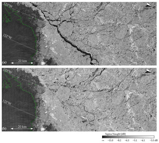
Figure 1.
TerraSAR-X ScanSAR images taken over the Canadian Arctic (Prince Patrick Island outlined in green). (a) SAR acquisition taken on 10 October 2010. (b) SAR acquisition taken on 11 October 2010. Sea ice floes with individual textures are recognizable. Changes in the sea ice due to drift are particularly visible in the open lead in the center of the image (slightly diagonal from top left to bottom right), which was closed on 11 October.
In order to automatically extract high-resolution sea ice drift vector fields from such SAR image pairs, and—in a second step—detect newly occurred deformation zones, an abundance of approaches have been investigated over the last few decades. Essentially, they can be split into (a) approaches relying on radar intensity or (b) approaches utilizing the interferometric SAR phase.
Algorithms that make use of the radar intensity include (i) feature tracking, (ii) optical flow and (iii) correlation-based techniques. Approaches using feature tracking, for example [3,4,5], first calculate certain local features and subsequently match the features from consecutive SAR acquisitions by following some criteria. The tracking can be based on pixel patterns [6] or on pre-classified objects [7]. In reference [4], a comprehensive overview of different feature tracking techniques is given. Algorithms that measure optical flow compute partial derivatives of the image signal [8,9]. Correlation-based techniques, namely algorithms that rely on the frequency-domain representation of the image (such as phase correlation or normalized cross correlation), are well established in a broad range of application areas, e.g., medical image processing, optical positioning and computer vision. It is used for SAR-based sea ice motion tracking [10,11] and is integrated in operational services [12,13,14]. Unlike many spatial-domain algorithms, the phase correlation method is quite resilient to overall brightness changes and noise [15] and requires little computing time. These properties make phase correlation a powerful tool for extracting sea ice drift vector fields. Furthermore, it can be used with SAR image pairs that differ in incidence angle range, orbit/heading angle, imaging mode and bands and even missions [11,16].
Combinations of feature tracking and phase correlation are presented in references [10,17]. They offer the possibility of combining the respective advantages of the individual methods and thus increase the overall reliability of the drift vector estimation. In our future work, we aim for such a combined processor.
On the other hand, there are approaches from SAR interferometry to characterize sea ice drift and detect landfast ice. Single-pass interferometry with bistatic satellite constellations such as TanDEM-X can determine sea ice drift velocities with high accuracy, but such data is not frequently available [18]. Differential repeat-pass interferometry uses the phase difference and coherence of at least two repeat-pass acquisitions and is therefore applicable to a wide range of SAR satellites with precise orbit information. It can be used to characterize sea ice deformation [19], identify cracks [20] and precisely evaluate landfast ice areas [21]. However, reliable interferometric phase analysis requires high coherence between image pairs, which is not always given. In particular, after storm events, when up-to-date sea ice information is most important for maritime users, the interferometric coherence of the sea ice surface can be significantly reduced. In addition, suitable interferometric SAR data from satellite repeat passes are also not frequently available.
Our work is focused on supporting operational services such as the German ice service at the BSH (Federal Maritime and Hydrographic Agency). Therefore, we need to fulfil NRT requirements and aim for approaches that allow frequent updates of the derived sea ice information. Interlinking SAR data of different satellite missions allows us to increase the update frequency. Hence, we primarily apply the phase correlation technique but use interferometry for comparison and cross-validation. In references [11,16], we showed successful results of our sea ice drift retrieval processor combining TerraSAR-X ScanSAR and RADARSAT-2 ScanSAR Wide acquisitions. In reference [22], we published a first validation study and presented an extensive validation using >1000 buoy measurements and a series of Sentinel-1 SAR data in reference [23].
In this paper, we analyze the localization accuracy of deformation zones in more detail. Therefore, we use drift buoys and observe landfast ice boundaries, as these represent a special type of deformation zone. To all our knowledge, only little research has been done on this particular topic. In reference [13], the landfast ice zones mapped by the Finnish and Swedish ice services are compared with the landfast ice boundaries that were automatically determined using phase correlation techniques. But the observed differences were attributed to a more critical assessment of the landfast ice zones by the ice services.
In our study, we investigate three different Arctic regions of interest (shown in Figure 2), each monitored on an approximately daily basis in TerraSAR-X SC mode. The first acquisition series was taken off the Eastern Greenland coast during winter, capturing landfast ice as well as drift ice. The second was taken over the Central Arctic, showing nothing but drift ice. The third monitors the Cardigan Strait (Canadian Arctic) during spring sea ice break up. We quantify the accuracy of retrieved sea ice drift vector fields using drift buoys (data provided by Environment Canada and the Alfred Wegener Institute for Polar and Marine Research) located in the SAR image footprints as well as manually outlined landfast ice boundaries. Furthermore, the interferometric coherence of SAR acquisitions from the Copernicus Sentinel-1 mission is used to cross-validate the landfast ice boundary.
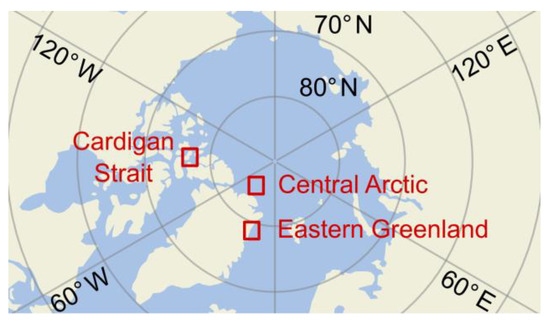
Figure 2.
Location of three regions of interest investigated in this study.
This paper is structured as follows. In Section 2, we briefly describe the basic principle of phase correlation techniques for image registration as well as our specific implementation for sea ice drift retrieval. The experimental results are given in Section 3. Afterwards, in Section 4, we cross-validate the experimental results with an interferometric analysis of the SAR data, focusing on the detection of landfast ice.
2. Sea Ice Drift Retrieval
2.1. Basic Concept of Phase Correlation
Assume two images, each with a size of pixels, that show the same object (such as the same piece of an ice sheet) but shifted by an unknown displacement vector and rotated by an unknown rotation angle. Translation, rotation and scaling have their equivalents in the frequency domain. That is, the unknown translation, rotation and scaling parameters can be efficiently determined by applying a Fourier transform to the images. Since only the knowledge of the translation parameters is required for the pure tracking of drifting sea ice, the phase correlation technique can be applied. Phase correlation is known to be resilient to rotation, overall brightness changes and noise. Different scaling does not come into play, as the input images are georeferenced.
Phase correlation relies on the shift theorem. Let the two images and be shifted versions of each other, that is
The Fourier transforms are then related as follows. When and denote the Fourier transforms of and , respectively, the following equation holds:
That is, the Fourier transforms of the two images and differ only by a change in the phase that is directly related to the translation . To extract the translation information from the pair of Fourier transforms, we can use the normalized cross power spectrum defined as
The inverse Fourier transform of is called the normalized cross correlation and shows a distinct peak indicating the translation parameter or displacement vector (u, v):
Figure 3 exemplarily shows the normalized cross correlation r (on the right) of two input images g and h (on the left). The displacement of the images results in a bright spot in the cross spectrum.
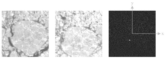
Figure 3.
Image patches the size of 16.9 km × 16.9 km cut out from the two spaceborne SAR acquisitions shown in Figure 1. The center coordinate of both image patches is 76.600°N, 123.081°W. They capture sea ice, which drifted down and slightly to the left (image coordinate system). Small features in the sea ice allow us to track them at a fine scale. The shift becomes visible in a bright spot in the normalized cross correlation (on the right).
The following section describes how to apply the above-mentioned basic concept of phase correlation to sequential, collocated SAR acquisitions to determine a two-dimensional sea ice drift vector field with an appropriate resolution.
2.2. Implementation of Phase Correlation for Sea Ice Drift Retrieval
Figure 4 illustrates the general workflow of our implementation. Firstly, from two input intensity images and , square image patches must be cut out. We introduce the following notation:
with and both ranging from to and denoting the patch center position (or drift vector starting point). The drift vector (u, v) is initialized as Then, the Hann function [24] is applied to both patches to prevent discontinuities at the patch boundaries when performing the discrete Fourier transform. From the Fourier-transformed images, the normalized cross correlation is computed. Following Equation (4), the position of the maximum is selected to update the drift vector (u, v).
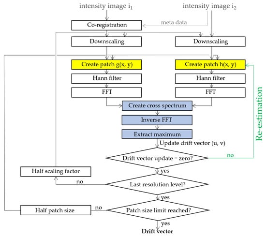
Figure 4.
Flow chart of the sea ice drift retrieval.
The estimation of the drift vector (u, v) is then repeated with new cut-outs from image (at the current drift vector ending points) until the estimation indicates an update of zero for both components u and v, which means that the optimal pattern match has been found. This re-estimation step (highlighted in green in Figure 4), inspired by the consistency check of [25], ensures a high similarity of the image patches and thus improves the estimation results.
To cover the entire SAR image footprint, the patch center position (, ) is changed according to the desired spacing of the drift vector field and the above procedure is repeated for each location. In the experimental results presented here, we use a drift vector spacing of 264 m. Figure 5 exemplarily shows the sea ice drift vector field retrieved from the TerraSAR-X acquisitions depicted in Figure 1. The sea ice drift velocity is indicated by colors, while arrows show the direction of the drift (in 3 km spacing). Color jumps in the velocity map indicate the convergence and divergence zones.
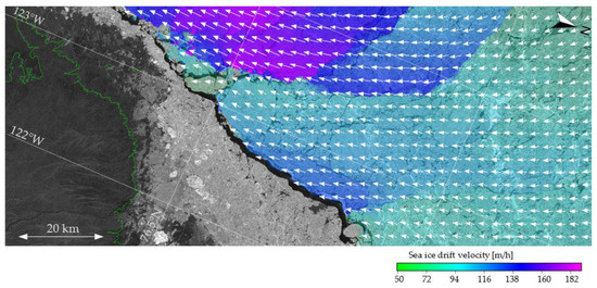
Figure 5.
Sea ice drift vector field derived from the TerraSAR-X image pair shown in Figure 1. Overlaid colors represent retrieved sea ice drift velocity in 264 m resolution and arrows illustrate sea ice drift direction (with 3 km sampling interval for illustration). Convergence and divergence zones become visible at the color jumps in the drift velocity map.
2.3. Patch Sizing
Attention must be paid to the selection of a suitable patch size . Large patches might cover areas with different drift motions, which leads to ambiguous results. Small patches may not cover large motions of the sea ice. A common approach to solving this problem is a hierarchical concept that starts with large patches to find large displacements and a subsequent stepwise reduction of the patch size. In our implementation, we repeat the drift vector field estimation in each layer of a multi-resolution Gaussian image pyramid with a reduction factor of 2 (see reference [13]). The size of the patches is kept constant at pixels, so the coverage is high at the coarsest resolution and is halved with each higher-resolution layer.
2.4. Limitations Due to the Patch Size
Still, small patches may cover multiple motions, especially when located in deformation zones or at the boundary of landfast ice. In these locations, at least two motions are covered by the patch, which theoretically results in two peaks (see Figure 6). We pick out the highest peak only, which represents the drift that is supported most, but not necessarily the drift of sea ice in the center of the patch. That is, based on the theory, deformation zones cannot be perfectly localized within the patch. Further reduction of the patch size is not practical as the drift estimation needs some distinctive features (distinguishable from noise), which disappear in smaller patches. We plan to analyze the secondary maxima in the cross spectrum in our future work. Up until now, we have quantized and analyzed the behavior of the current available implementation.
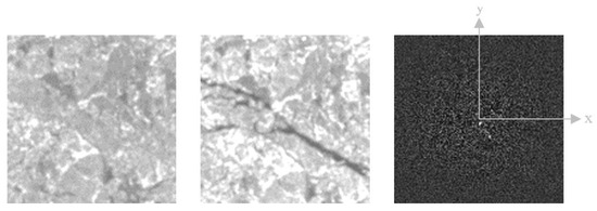
Figure 6.
Image patches the size of 8.4 km × 8.4 km cut out from the two spaceborne SAR acquisitions shown in Figure 1. The center coordinate of both image patches is 77.034°N, 125.155°W. They capture sea ice with two different motions, which cause the occurrence of a new open lead. Above the open lead, the sea ice hardly drifted. Below the open lead, the sea ice drifted to the bottom right (image coordinate system). These two motions result in two bright spots in the normalized cross correlation (on the right). The brighter spot corresponds to the ice above the open lead.
2.5. Landfast Ice Detection Based on the Retrieved Sea Ice Drift Field
Based on the estimated sea ice drift vector field, we determine the extent of possible landfast ice zones. Therefore, a simple region-growing procedure is performed starting from the coast, including all drift vectors with a magnitude below a certain threshold T. Our experimental results define a reasonable threshold as well as document the localization accuracy of detected landfast ice boundaries compared to manually outlined landfast ice zones.
3. Experimental Results
In order to quantify the accuracy of the above-mentioned sea ice drift retrieval algorithm, we used drift buoy data provided by Environment Canada (buoy 300234060838110) and the Alfred Wegener Institute (buoy 300234064138630) as well as TerraSAR-X SC acquisitions taken over these buoys. The time difference between subsequent SAR acquisitions varies from a few hours to a few days. We selected two study areas including drift buoys and a third study area capturing landfast ice break-off.
The first study area is located off the Eastern Greenland coast (at center coordinate 78.463°N 16.926°W) and the second is in the Central Arctic (at center coordinate 85.563°N 49.793° W). The Eastern Greenland time series includes 21 individual SAR acquisitions taken between 15 and 31 January 2018 and covers both landfast ice and drift ice, as well as drift buoy 300234060838110. The Central Arctic time series includes drift buoy 300234064138630, which was deployed during the IceBird 2017 campaign [26] and captures nothing but drift ice within the footprint margins. Here, 38 images were acquired between 3 and 31 March 2018.
The considered drift buoys recorded their positions on an hourly basis via GPS. We approximated the buoy positions for the given SAR acquisition time using linear interpolation and set the drift vector starting point to that approximated coordinate. We compared the resulting drift vector ending points with the approximated buoy position at the later SAR acquisition time, and calculated the absolute error Δs (see Figure 7). Not only were subsequent SAR acquisitions considered, but also all possible scene combinations up to a time difference of 16 days.
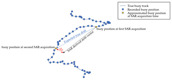
Figure 7.
Definition of the absolute error Δs.
To observe the landfast ice boundary, we used the above-mentioned Eastern Greenland time series as well as a time series of TerraSAR-X SC acquisitions taken over our third study area, which monitors the Cardigan Strait (at center coordinate 76.999°N 91.707°W). The Cardigan Straight time series consists of 148 acquisitions taken from 26 April to 25 September 2021 and captures landfast ice break-off.
All tests were run with four layers of the Gaussian image pyramid, while the highest resolution still uses a scaling factor of 2 due to speckle noise removal. Thus, the image resolution in the last processing step is 33 m and the pixel spacing is 16.5 m. N is set to 128 pixels. The estimation starts from patches with a size of 16.9 km × 16.9 km, and ends with a size of 2.1 km × 2.1 km.
In the following section, Section 3.1, we evaluate the accuracy of the sea ice drift vector estimation focusing on consolidated sea ice. The accuracy in deformation zones is examined separately in Section 3.2.
3.1. Accuracy of the Drift Retrieval Within Consolidated Sea Ice
3.1.1. Buoys over Unmoved Ice
In 26 TerraSAR-X image pairs (23 from the Eastern Greenland time series and 3 from the Central Arctic times series), the observed buoy did not move, resulting in 26 measurement values for which the absolute error Δs was analyzed. These unmoved buoys form the first part of our analysis.
Due to the limited number of measurements, we manually picked out five locations spread across the landfast ice zone in the Eastern Greenland study area, and created five (emulated) buoy data sets for these locations, resulting in 381 additional measurements for which the absolute error Δs was also examined.
Figure 8 shows the measured absolute error Δs as a function of the time difference between the SAR image acquisitions. The absolute error ranges from 0 m to 45 m. On average, it is 12.3 m. Even the highest measured value of 45 m is relatively low compared to the image resolution of 33 m.
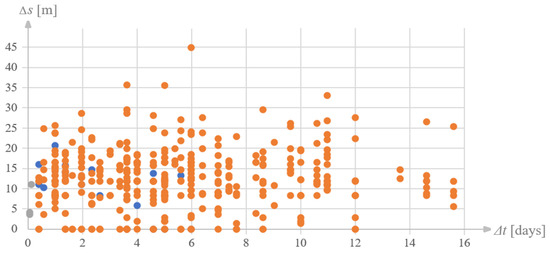
Figure 8.
Absolute error Δs versus time difference Δt between two SAR acquisitions (Eastern Greenland and Cardigan Strait time series). Blue: measurements using buoy data of Eastern Greenland time series. Grey: measurements using buoy data of Central Arctic time series. Orange: measurements using emulated buoy data of Eastern Greenland time series.
There is hardly any dependence on the time difference visible in Figure 8, but larger data sets show that the absolute error increases with increasing time difference due to erosion on the sea ice and changes in radar backscatter caused by melting or precipitation (see next section).
3.1.2. Buoys’ over Drift Ice
The second part of our analysis concentrates on buoys’ over drift ice (from the Central Arctic time series). A total of 273 measurements yielded a sea ice displacement of up to 8.45 km. This value is set as the limit, as this is half the patch size in the first estimation loop. All displacements that exceed half the patch size can hardly be recognized with block-based pattern matching techniques.
In Figure 9, the absolute error is shown as a function of the sea ice displacement (distance) between the buoy positions of the first and second SAR acquisition. The greater the distance, the more deformations occur, and the lower the accuracy of the sea ice drift vector estimation is. The highest measured absolute error is 130 m (for 8.4 km sea ice displacement). Most absolute errors are below 100 m.
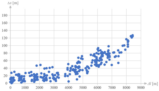
Figure 9.
Absolute error Δs versus absolute sea ice displacement Δl measured using buoys located in the Central Arctic time series.
Figure 10 shows the absolute error as a function of the time difference between two SAR acquisitions. In contrast to Figure 8, the expected dependency on time difference is visible. Processes such as erosion or precipitation affect the radar backscatter at the sea ice surface, and thereby change the patterns needed for drift tracking. With time, these influences increase and result in an increase in the absolute error. In other words, the smaller the time difference between two SAR acquisitions and the smaller the absolute sea ice drift, the better the estimation of a sea ice drift vector field. In good circumstances, a sub-pixel accuracy (more precisely, an absolute error below 33 m) is achieved.
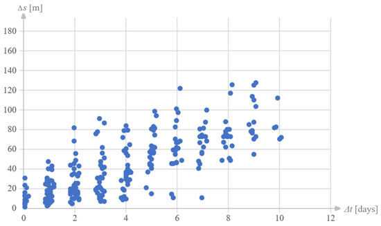
Figure 10.
Absolute error Δs versus time difference Δt between two SAR acquisitions (Central Arctic time series).
3.2. Accuracy in Deformation Zones
The analysis in Section 3.1 shows that the sea ice drift retrieval is most reliable when the absolute sea ice displacement captured from two SAR acquisitions is small and the time difference between these acquisitions is small. Higher sea ice displacements result in larger errors. But over landfast ice, we can expect very high reliability, especially when the time difference between the selected SAR acquisitions amounts to a few days only. Based on the buoy validation presented in Section 3.1, we set the threshold for landfast ice detection to T = 200 m.
However, the buoys are placed within consolidated sea ice and therefore cannot be used to quantify the accuracy of the drift retrieval in deformation zones. Therefore, we analyzed the localization accuracy of the (changing) landfast ice boundary captured from the SAR acquisitions in our Cardigan Straight and East Greenland times series. We picked out selected examples to discuss the behavior of our sea ice drift retrieval method.
3.2.1. Sea Ice Break-Off
From our Cardigan Straight time series, several major sea ice break-offs can be observed. One occurred between 29 June 2021 12:39 UTC and 29 June 2021 23:36 UTC and resulted in an open lead nearly 2 km wide. Figure 11 shows sections from both SAR acquisitions and, superimposed in yellow, the landfast ice boundary which was automatically generated after sea ice drift retrieval. Apart from some fraying, it coincides reasonably well with the visible boundary of the landfast ice. Deviations can be attributed to the drift estimation method focusing on the predominant drift component within each patch: Patches that mainly cover landfast ice result in a low drift magnitude close to zero. Patches that mainly cover either the newly occurred open lead or the broken ice generate a drift vector that describes the drift (magnitude ~2 km).
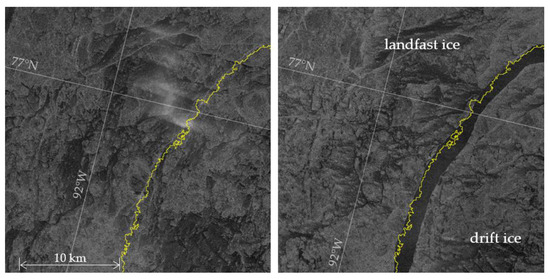
Figure 11.
Sections from a TerraSAR-X image pair acquired on 29 June 2021 12:39 UTC (left) and 29 June 2021 23:36 UTC (right) from before and after a major sea ice break-off event. The landfast ice boundary was detected using the phase correlation technique.
3.2.2. Stable Landfast Ice Boundary with Drift Ice at Some Distance
After the sea ice break-off that happened on 29 June 2021, the resulting ice floe remained relatively stationary for a while. More precisely, between 29 June 2021 23:36 UTC and 30 June 23:19 UTC, it mainly rotated, resulting in a sea ice displacement of about 600 m at the ice edge, and no displacement in the middle of the floe. The landfast ice did not change. As visible in Figure 12, the automatically generated landfast ice zone is oversized. Its detected boundary is located in the middle of the open lead and not at the ice edge. This is because the ice edge of the landfast ice has remained unchanged and all patches that cover a major part of either landfast ice or open water with only a minor portion of landfast ice result in a drift vector magnitude of approximately zero. In contrast, all patches that cover a major part the drift ice or open water with only a small portion of drift ice yield a drift vector of the order of 600 m.
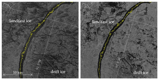
Figure 12.
Landfast ice detection from a TerraSAR-X image pair acquired on 29 June 2021 23:36 UTC (left) and 30 June 2021 23:19 UTC (right) showing a stable landfast ice boundary. The automatically detected landfast ice is oversized.
To sum up, a block-matching approach that searches for one maximum in the cross correlation has limitations when it comes to deformation zones but makes drift retrieval more robust. In general, deformation zones can be localized with an accuracy that is in the range of the half patch size.
3.2.3. Stable Landfast Ice with Drift Ice Passing by
Our East Greenland times series captures drift ice that borders the landfast ice zone. Figure 13 shows a section from the TerraSAR-X SC acquisitions taken on 16 January 2018 17:26 UTC and 19 January 2018 08:46 UTC, where the landfast ice boundary is approximately vertical, and drift ice on the right-hand site is moving down (image coordinate system). The automatically generated landfast ice boundary represents the real landfast ice boundary quite well. Patches that cover both the landfast ice and the drift ice produce a drift vector magnitude of ~0 if landfast ice dominates, and a drift vector magnitude of >0 if drift ice dominates in the respective patches.
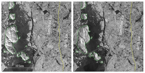
Figure 13.
Drift ice drifting parallel to the landfast ice boundary, captured from a TerraSAR-X image pair acquired on 16 January 2018 17:26 UTC (left) and 19 January 2018 08:46 UTC (right). The yellow line indicates the automatically generated landfast ice boundary. Green lines mark the coastline. The landfast ice boundary is detected well using the phase correlation technique.
In summary, in many cases deformation zones can be easily identified using the phase correlation method. Under certain circumstances, the position of the deformation zones may be shifted. The shift depends on the final patch size, and in the worst case, is in the order of half side length, which is about 1 km in our implementation.
3.3. Observation of the Landfast Ice Boundary
In Section 3.1 and Section 3.2, the performance of our sea ice drift retrieval is demonstrated using selected examples. To give a broader view, Figure 14 summarizes the landfast ice boundaries generated from the TerraSAR-X acquisitions of the Eastern Greenland times series, and in addition, landfast ice boundaries derived from collocated Sentinel-1 images. Overall, the whole Eastern Greenland study area was densely covered by sea ice that mostly remained stationary, especially from 22 to 31 January 2018. At a ~60 km distance to the coast, a large open lead can be observed. This open lead opened up in several steps, followed by refreezing. Beyond the open lead, the sea ice underwent significant changes during the observation period, but the ice between the coast and the open lead was unchanged and motionless. Our sea ice drift retrieval detects the open lead and the small changes around it well (see blue and green lines in Figure 14). However, the sea ice up to the lead is likely unstable and may not be anchored to the land. TerraSAR-X acquisitions taken on 21 and 22 January 2018 capture a landfast ice break-off quite close the coast (see red line in Figure 14). Also, from the Sentinel-1 image pair taken on 17 and 29 January 2018, a landfast ice boundary in proximity to the land can be determined (dashed orange line in Figure 14), which aligns closely with the TerraSAR-X-based retrieval. The recorded motion is not large (only around 250 m in magnitude) but spans nearly the entire sea ice in the footprint. After this break-off event, the sea ice moved back, and stayed unmoved, but one can assume that the stability of the sea ice has decreased. This leads to the conclusion that for operational landfast ice detection, a time series of multiple image pairs must be examined.
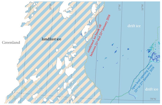
Figure 14.
Landfast ice boundaries captured from different TerraSAR-X and Sentinel-1 image pairs acquired between 17 and 29 January 2018 off the Eastern Greenland coast. The light-yellow striped area marks the manually labeled landfast ice zone. It coincides well with the landfast ice boundary generated from the TerraSAR-X image pair taken on 21 and 22 January 2018 (red line) and from the Sentinel-1 image pair taken on 17 and 29 January 2018 (dashed orange line). From 22 to 29, the image footprints were covered throughout by unmoved ice, apart from an open lead at a 60 km distance to the coast, which opened up and refroze in several steps. These openings and closings are captured in the TerraSAR-X image pairs taken on 22 and 24 January 2018 (dark blue line), 24 and 25 January 2018 (cyan line) and 26 and 27 January 2018 (turquoise line) and from the Sentinel-1 image pair taken on 23 and 29 January 2018 (dashed green line), but does not represent the border of the landfast ice zone.
In the Eastern Greenland study area, there is no publicly available ground truth data on the extent of the landfast ice. In the following section, we therefore cross-validate the results of our phase-correlation-based sea ice drift retrieval with an independent method based on differential SAR interferometry.
4. Interferometric Detection of Landfast Ice
In the last chapter, a method for sea ice drift retrieval based on radar intensity was introduced. In contrast, differential SAR interferometry exploits the phase change of satellite repeat passes to map ground deformations and displacements [27]. In the cryosphere, this allows us to measure glacier flow velocities [28,29], analyze sea ice deformations [19], identify cracks [20] and detect landfast ice [21]. In this work, interferometry is used to validate the performance of the intensity-based sea ice drift retrieval demonstrated in Section 3.
The temporal baseline of the interferometric method is set by the orbit repeat cycle of the satellite constellation, which is 11 days for TerraSAR-X (X-band). In comparison, the Sentinel-1 C-band SAR mission has a repeat cycle of six days when combining Sentinel-1A and 1B, depending on the area of interest. Due to the fixed schedule of Sentinel-1 acquisitions, the shorter repeat cycle and the lower temporal decorrelation in C-band, Sentinel-1 imagery is chosen for the interferometric analysis.
The image pairs are geometrically co-registered with ESA SNAP using precise orbit information and a digital elevation model. An interferogram is then created by evaluating the complex backscatter amplitudes and of the primary and secondary acquisition, respectively. The accuracy of the interferogram is characterized by the absolute value of the coherence which is evaluated in a fixed window around the point of interest :
Several processes lead to a decorrelation of the two acquisitions. In the field of landfast ice detection, the temporal decorrelation is used to distinguish stationary ice (high coherence) from drift ice (low coherence) in order to compute the landfast ice boundary. A high coherence contrast requires favorable conditions without precipitation, erosion and melting.
4.1. Interferometric Coherence as a Measure for Landfast Ice
The Eastern Greenland study area is chosen to demonstrate the interferometry-based method for detecting landfast ice. Two Sentinel-1 Interferometric Wide Swath (IW) acquisitions form the interferometric image pair, taken on 23 January 2018 08:34 UTC and 29 January 2018 08:34 UTC, that is, one before and one after the break-off of the large open lead at a 60 km distance to the coast (see the dashed green line in Figure 14). According to ECMWF ERA5 reanalysis data [30], there was no precipitation and the temperatures remained below −10 °C between the two acquisitions.
Figure 15a shows the interferogram of the image pair overlaid with the land area. The interferogram was filtered using the adaptive method introduced by Goldstein [31] and smoothed for better visualization. Areas of high fringe density are related to deformations within the ice. Perturbations and discontinuities in the fringe pattern indicate ice ridges and cracks [19,20,32]. The coherence is shown in Figure 15b. A coherence window of 10 px in range and 3 px in azimuth, corresponding to 43 m × 42 m on ground, is chosen as a compromise between noise suppression and spatial resolution.
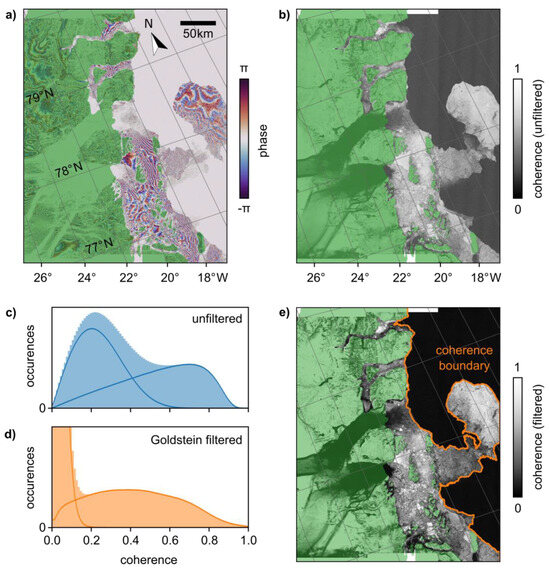
Figure 15.
Interferometry-based determination of the landfast ice boundary in the Eastern Greenland study area. (a) The interferogram and (b) coherence of the Sentinel-1 scene pair 23 and 29 January 2018. The land area is shaded in green. (c,d) Histograms of the (c) unfiltered and (d) filtered coherence from no-land areas. The solid lines show the contributions from stationary and moving ice. (e) The Goldstein-filtered coherence and automatically derived coherence boundary, separating landfast and drifting ice.
The scene is almost completely covered by land and sea ice. Low-coherence areas in the left part of the image, mostly on land, are related to the Zachariæ Isstrøm glacier flow, which terminates on the sea ice. In the right part of the image, the low-coherence areas indicate significant sea ice drift on the order of the pixel size or larger. In contrast, landfast ice manifests as high-coherence areas where the ice remained stationary between the two acquisitions. In the following, the line separating the high- and low-coherence areas will be determined to map the landfast ice boundary.
4.2. Automated Detection of the Landfast Ice Boundary
Figure 15c shows the histogram of the coherence values for all non-land areas. The two peaks in the histogram, corresponding to drifting and landfast ice, are broad and overlap significantly. As demonstrated by reference [21], an adaptive spatial filtering of the coherence allows the two peaks to be further separated.
The Goldstein filtering method was originally developed as an adaptive filter for interferograms but can be applied to any complex spatial data . The input data is filtered by a sliding window of fixed size, for example 64 × 64 pixel. We denote the Fourier transform over such a window by . The absolute value of this spectrum is smoothed by a moving average filter , yielding . The filter function is then constructed as , where determines the filter strength. After applying the inverse Fourier transform to the scaled spectrum, we obtain the filtered data .
We choose a 64 × 64-pixel Fourier window, a 3 × 3-pixel smoothing kernel and the filter parameter . We filter the numerator and the two parts of the denominator of Equation (7) individually and obtain the spatially filtered coherence shown in Figure 15e. The corresponding histogram in Figure 15d illustrates that the adaptive filtering significantly decreased the mean and width of the low-coherence peak and allows a better separation of stationary and drifting image components.
For further analysis, the image is downscaled by a factor of 3 in the range direction, resulting in approximately square pixels with an edge length of about 14 m. Based on the position of the local minimum between the low-coherence and high-coherence peaks in the histogram, we first apply a threshold of to the filtered coherence. Although an adaptive CFAR-based coherence threshold was used in reference [21], we choose a static threshold due to the narrow low-coherence peak in the histogram. The binary mask is then refined through a series of morphological operations to map the landfast ice area. The steps are binary closing, removal of small holes, binary opening and removal of small objects. The low-coherence area associated with glacier flow is manually removed from the binary mask.
The solid lines in the histograms in Figure 15c,d depict the contributions from stationary and moving ice before and after coherence filtering. The asymmetry of the high-coherence peak is caused by multiple contributions from different areas in the landfast ice. The orange line in Figure 15e shows the resulting landfast ice boundary, which clearly separates the low- and high-coherence areas.
In particular, two effects influence the accuracy of the landfast ice boundary and its comparability with other approaches. First, our approach is based on a purely geometric co-registration. Therefore, ice movement on the order of the pixel size (about 14 m) or more leads to decorrelation, which we then consider drifting ice. Second, the inevitable noise in the spatial coherence data introduces uncertainties in the position of the derived landfast ice boundary. Considering the size of the coherence window (42 m) and the kernels used for the morphological operations (140 m), we estimate the positional accuracy to be around 200 m.
4.3. Comparison with the Intensity-Based Sea Ice Drift Retrieval
Due to the high spatial resolution of the interferometric data, the landfast ice boundary serves as a good benchmark for the previously introduced intensity-based sea ice drift determination. The ice break-off events were already analyzed with intensity images from TerraSAR-X and Sentinel-1 in Section 3.3.
Figure 16 compares the sea ice drift magnitude derived from the phase-correlation-based approach with the interferometric landfast ice boundary. The drift field reveals a strong ice movement of more than 100 m in the eastern part of the image, following the major ice break-off event, while the blue areas in the figure denote stationary ice.
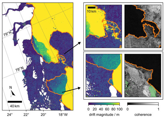
Figure 16.
Comparison of the intensity-based sea ice drift magnitude with the interferometry-based landfast ice boundary (orange line) in Eastern Greenland. The land area is marked in white. The right part shows the details of the areas marked by the black arrows, comparing the sea ice drift magnitude and the interferometric coherence.
As discussed in Section 3.1.1, the uncertainty of the drift magnitude on unmoved ice is up to 45 m for TerraSAR-X data, and up to 125 m for Sentinel-1 data (see our previous analysis in reference [23]). Based on these numbers, the interferometry-based landfast ice boundary generally agrees well with the boundaries of the intensity-based drift magnitude.
There are two large areas with intermediate drift magnitudes on the order of 40 m which are not considered landfast ice in the interferometric results. These two areas are shown in detail in the right part of Figure 16 and compared with the coherence map. The southern area underlines the high sensitivity of the interferometric approach. The comparison with the coherence of the same area shows a good agreement between the two methods. Notably, the interferometric approach identified the ice break-off that occurred between 21 and 22 January 2018 (compare the dashed orange line in Figure 14), which happened before the interferometric image pair was acquired, as the landfast ice boundary. The instability of the ice and the small movements (≪100 m) that followed the break-off are within the range of uncertainty of the intensity-based approach, but they can be detected well by interferometry.
The northern area illustrates a complex ice movement. In this area, the coherence contrast is rather weak, probably because the ice movement is close to the resolution and sensitivity limit of our interferometric approach. Consequently, the landfast ice boundary has a higher uncertainty, which is also shown in the intensity-based drift results as small patches with high drift and low drift magnitudes.
5. Discussion
Phase correlation is commonly used for operational sea ice drift retrieval from spaceborne SAR acquisitions. In order to evaluate the capabilities of phase correlation in more detail, we used TerraSAR-X ScanSAR image time series taken over three Arctic regions and drift buoys located in the SAR image footprints. Overall, we found that the accuracy of our implementation is notably high within consolidated ice. It is below 45 m for stationary sea ice, and below 130 m for drifting ice. In optimal conditions, a sub-pixel accuracy is obtained. The accuracy decreases with larger sea ice displacement and longer time intervals between the image pairs. This can be attributed to processes such as erosion, melting or precipitation, which alter the radar backscatter and thus complicate pattern recognition.
In addition to the drift buoy evaluation, we observed the landfast ice boundary which was manually delineated from TerraSAR-X ScanSAR and Sentinel-1 IW acquisitions. The landfast ice boundary is considered to be a distinct category of deformation zone. We noted that, in contrast to the drift within consolidated ice, deformation zones may be mispositioned, as phase correlation requires image patches of a given size in order to discern patterns. The normalized cross correlation reveals several maxima in image patches depicting various sea ice regions moving in different directions and/or at different speeds, with each maximum corresponding to one distinct motion. In our implementation, we select the most dominant maximum, as this enhances the robustness of the sea ice drift retrieval. However, this choice constrains the accuracy of deformation zone localization. Assuming two motions in one image patch lead to two maxima, we can roughly estimate that the more dominant maximum represents over 50% of the sea ice captured in that patch. Consequently, the displacement of deformation zones can reach approximately half the size of the patch, which amounts to 1.1 km in this implementation.
For comparison and cross-validation purposes, we extended our analysis of the intensity-based landfast ice detection with an approach based on Sentinel-1 repeat-pass interferometry. Overall, our study revealed a very good agreement between the two complementary approaches. The interferometric approach generally provides a more conservative estimate of landfast ice areas, exhibiting high sensitivity and a high localization accuracy of around 200 m under optimal conditions.
However, the interferometric approach is more susceptible to unfavorable weather conditions, such as precipitation and melting, than the intensity-based approach. Consequently, the interferometric approach is less likely to produce timely and applicable results when the landfast ice boundary has changed, for example after a storm event. In such cases, the intensity-based approach is more robust.
Furthermore, the intensity-based phase correlation technique is not limited to satellite repeat passes. It can be applied to image pairs from different orbits, different incidence angle ranges and even different bands and missions. Therefore, the intensity-based approach enables sea ice analysis at considerably shorter time intervals and is, at present, more appropriate for operational applications.
Author Contributions
Conceptualization, A.F. and C.S.; methodology, A.F., C.S. and S.R.; software and validation, A.F., C.S. and S.R.; formal analysis and investigation, all authors; data curation, A.F., C.S. and S.R.; writing—original draft preparation, A.F. and C.S.; writing—review and editing, all authors; visualization, all authors; supervision, all authors; project administration, A.F. All authors have read and agreed to the published version of the manuscript.
Funding
This research received no external funding.
Data Availability Statement
Figure 15 and Figure 16 contain modified Copernicus Sentinel data (2018). The Sentinel-1 data presented in the study can be obtained free of charge from the Copernicus Dataspace at https://dataspace.copernicus.eu (accessed on 23 October 2024). The TerraSAR-X ESA Archive is freely available to download for anyone with an account in ESA’s EO Sign In service. Further material presented in the study can be requested from the corresponding author.
Conflicts of Interest
The authors declare no conflicts of interest.
Abbreviations
The following abbreviations are used in this manuscript:
| NRT | Near Real-Time |
| SAR | Synthetic Aperture Radar |
| SC | ScanSAR (mode of TerraSAR-X) |
| IW | Interferometric Wide Swath (mode of Sentinel-1) |
References
- Dierking, W. Mapping of different sea ice regimes using images from Sentinel-1 and ALOS synthetic aperture radar. IEEE Trans. Geosci. Remote Sens. 2009, 48, 1045–1058. [Google Scholar] [CrossRef]
- Eineder, M.; Fritz, T.; Mittermayer, J.; Roth, A.; Boerner, E.; Breit, H. TerraSAR-X Ground Segment, Basic Product Specification Document; Report No. TX-GS-DD-3302; Cluster Applied Remote Sensing (CAF): Oberpfaffenhofen, Germany, 2008. [Google Scholar]
- Kwok, R.; Curlander, J.C.; McConnell, R.; Pang, S. An Ice Motion Tracking System at the Alaska SAR Facility. IEEE J. Ocean. Eng. 1990, 15, 44–54. [Google Scholar] [CrossRef]
- Muckenhuber, S.; Korosov, A.A.; Sandven, S. Open-source feature-tracking algorithm for sea ice drift retrieval from Sentinel-1 SAR imagery. Cryosphere 2016, 10, 913–925. [Google Scholar] [CrossRef]
- Demchev, D.; Volkov, V.; Kazakov, E.; Sandven, S. Feature tracking for sea ice drift retrieval from SAR images. In Proceedings of the IEEE International Geoscience and Remote Sensing Symposium, Fort Worth, TX, USA, 23–28 July 2017; pp. 330–333. [Google Scholar]
- Fily, M.; Rothrock, D.A. Sea ice tracking by nested correlations. IEEE Trans. Geosci. Remote Sens. 1987, GE-25, 570–580. [Google Scholar] [CrossRef]
- Banfield, J. Automated tracking of ice floes: A stochastic approach. IEEE Trans. Geosci. Remote Sens. 1991, 29, 905–911. [Google Scholar] [CrossRef]
- Horn, B.K.P.; Schunck, B.G. Determining optical flow. Artif. Intell. 1981, 17, 185–203. [Google Scholar] [CrossRef]
- Sun, Y. Automatic ice motion retrieval from ERS-1 SAR images using the optical flow method. Int. J. Remote Sens. 1996, 17, 2059–2087. [Google Scholar] [CrossRef]
- Kwok, R.; Schweiger, A.; Rothrock, D.A.; Pang, S.; Kottmeier, C. Sea ice motion from satellite passive microwave imagery assessed with ERS SAR and buoy motions. J. Geophys. Res. Ocean. 1998, 103, 8191–8214. [Google Scholar] [CrossRef]
- Frost, A.; Jacobsen, S.; Singha, S. High resolution sea ice drift estimation using combined TerraSAR-X and RADARSAT-2 data: First tests. In Proceedings of the IEEE International Geoscience and Remote Sensing Symposium, Fort Worth, TX, USA, 23–28 July 2017; pp. 342–345. [Google Scholar]
- Karvonen, J. Operational SAR-based sea ice drift monitoring over the Baltic Sea. Ocean Sci. 2012, 8, 473–483. [Google Scholar] [CrossRef]
- Mäkynen, M.; Karvonen, J.; Cheng, B.; Hiltunen, M.; Eriksson, P.B. Operational service for mapping the Baltic Sea landfast ice properties. Remote Sens. 2020, 12, 4032. [Google Scholar] [CrossRef]
- Saldo, R. Global Ocean—High Resolution SAR Sea Ice Drift; Marine Data Store (MDS); E.U. Copernicus Marine Service Information (CMEMS): Toulouse, France, 2023. [Google Scholar] [CrossRef]
- Nithyanandam, S.; Amaresan, S.; Haris, N.M. An innovative normalization process by phase correlation method of Iris images for the block size of 32∗32. In Proceedings of the IEEE Fifth International Conference on the Applications of Digital Information and Web Technologies, Bangalore, India, 17–19 February 2014; pp. 189–194. [Google Scholar]
- Frost, A.; Wiehle, S.; Singha, S.; Krause, D. Sea ice motion tracking from near real time SAR data acquired during Antarctic circumnavigation expedition. In Proceedings of the IEEE International Geoscience and Remote Sensing Symposium, Valencia, Spain, 22–27 July 2018; pp. 2338–2341. [Google Scholar]
- Korosov, A.A.; Rampal, P. A combination of feature tracking and pattern matching with optimal parametrization for sea ice drift retrieval from SAR data. Remote Sens. 2017, 9, 258. [Google Scholar] [CrossRef]
- Dammann, D.O.; Eriksson, L.E.; Jones, J.M.; Mahoney, A.R.; Romeiser, R.; Meyer, F.J.; Eicken, H.; Fukamachi, Y. Instantaneous sea ice drift speed from TanDEM-X interferometry. Cryosphere 2019, 13, 1395–1408. [Google Scholar] [CrossRef]
- Dammann, D.O.; Eicken, H.; Meyer, F.J.; Mahoney, A.R. Assessing small-scale deformation and stability of landfast sea ice on seasonal timescales through L-band SAR interferometry and inverse modeling. Remote Sens. Environ. 2016, 187, 492–504. [Google Scholar] [CrossRef]
- Libert, L.; Wuite, J.; Nagler, T. Automatic delineation of cracks with sentinel-1 interferometry for monitoring ice shelf damages and calving. Cryosphere Discuss. 2021, 16, 1523–1542. [Google Scholar] [CrossRef]
- Meyer, F.J.; Mahoney, A.R.; Eicken, H.; Denny, C.L.; Druckenmiller, H.C.; Hendricks, S. Mapping arctic landfast ice extent using L-band synthetic aperture radar interferometry. Remote Sens. Environ. 2011, 115, 3029–3043. [Google Scholar] [CrossRef]
- Frost, A.; Wiehle, S.; Jacobsen, S. Accuracy of a Phase-Correlation Technique for Fully Auto-Mated Sea Ice Motion Retrieval Based on Sequential SAR Images; SeaSAR; Maritime Safety and Security Lab German Aerospace Center (DLR): Köln, Germany, 2018. [Google Scholar]
- Frost, A.; Imber, J.; Murashkin, D.; Gregorek, D.; Bathmann, M. Phase-Correlation Based Sea Ice Motion Tracking and Classification Using Spaceborne SAR Imagery. In Proceedings of the OCEANS Limerick, Limerick, Ireland, 5–8 June 2023; pp. 1–8. [Google Scholar]
- Blackman, R.B.; Tukey, J.W. “Particular Pairs of Windows” the Measurement of Power Spectra, from the Point of View of Communications Engineering; Dover: New York, NY, USA, 1959; pp. 14–15, 95–100. [Google Scholar]
- Hollands, T. Motion Tracking of Sea Ice with SAR Satellite Data. Ph.D. Thesis, Universität Bremen, Bremen, Germany, 2012. [Google Scholar]
- Krumpen, T.; Nicolaus, M. Sea Ice Drift and Surface Temperature from Autonomous Measurements from Buoy 2017C21, Deployed During IceBird 2017; PANGAEA: Bremen, Germany, 2018. [Google Scholar]
- Hanssen, R.F. Radar Interferometry: Data Interpretation and Error Analysis; Springer Science & Business Media: Berlin/Heidelberg, Germany, 2001; Volume 2. [Google Scholar]
- Goldstein, R.M.; Engelhardt, H.; Kamb, B.; Frolich, R.M. Satellite radar interferometry for monitoring ice sheet motion: Application to an Antarctic ice stream. Science 1993, 262, 1525–1530. [Google Scholar] [CrossRef] [PubMed]
- Ramanath, S.; Krieger, L.; Floricioiu, D.; Heidler, K. Deep learning based automatic grounding line delineation in DInSAR interferograms. Cryosphere Discuss. 2024. [Google Scholar] [CrossRef]
- Hersbach, H.; Bell, B.; Berrisford, P.; Biavati, G.; Horányi, A.; Muñoz Sabater, J.; Nicolas, J.; Peubey, C.; Radu, R.; Rozum, I.; et al. ERA5 Hourly Data on Single Levels from 1940 to Present; Copernicus Climate Change Service (C3S), Climate Data Store (CDS): Bonn, Germany, 2023. [Google Scholar] [CrossRef]
- Goldstein, R.M.; Werner, C.L. Radar interferogram filtering for geophysical applications. Geophys. Res. Lett. 1998, 25, 4035–4038. [Google Scholar] [CrossRef]
- Dammann, D.O.; Eicken, H.; Mahoney, A.R.; Meyer, F.J.; Freymueller, J.T.; Kaufman, A.M. Evaluating landfast sea ice stress and fracture in support of operations on sea ice using SAR interferometry. Cold Reg. Sci. Technol. 2018, 149, 51–64. [Google Scholar] [CrossRef]


Disclaimer/Publisher’s Note: The statements, opinions and data contained in all publications are solely those of the individual author(s) and contributor(s) and not of MDPI and/or the editor(s). MDPI and/or the editor(s) disclaim responsibility for any injury to people or property resulting from any ideas, methods, instructions or products referred to in the content. |
© 2025 by the authors. Licensee MDPI, Basel, Switzerland. This article is an open access article distributed under the terms and conditions of the Creative Commons Attribution (CC BY) license (https://creativecommons.org/licenses/by/4.0/).