Abstract
Desertification threatens the sustainability of dryland ecosystems, yet many existing monitoring frameworks rely on static maps, coarse spatial resolution, or lack temporal forecasting capacity. To address these limitations, this study introduces PyGEE-ST-MEDALUS, a novel spatiotemporal framework combining the full MEDALUS desertification model with deep learning (CNN, LSTM, DeepMLP) and machine learning (RF, XGBoost, SVM) techniques on the Google Earth Engine (GEE) platform. Applied across Tebessa Province, Algeria (2001–2028), the framework integrates MODIS and Sentinel-1/-2 data to compute four core indices—climatic, soil, vegetation, and land management quality—and create the Desertification Sensitivity Index (DSI). Unlike prior studies that focus on static or spatial-only MEDALUS implementations, PyGEE-ST-MEDALUS introduces scalable, time-series forecasting, yielding superior predictive performance (R2 ≈ 0.96; RMSE < 0.03). Over 71% of the region was classified as having high to very high sensitivity, driven by declining vegetation and thermal stress. Comparative analysis confirms that this study advances the state-of-the-art by integrating interpretable AI, near-real-time satellite analytics, and full MEDALUS indicators into one cloud-based pipeline. These contributions make PyGEE-ST-MEDALUS a transferable, efficient decision-support tool for identifying degradation hotspots, supporting early warning systems, and enabling evidence-based land management in dryland regions.
1. Introduction
Desertification significantly threatens global food security, ecosystem stability, and socioeconomic resilience, affecting over 40% of the world’s land classified as drylands. Driven by population growth, unsustainable agricultural practices, and climate change, land degradation has escalated notably in arid and semi-arid regions, which often lack sufficient infrastructural and economic resources, making them highly vulnerable to water stress and biodiversity loss [1,2,3]. Consequently, there is an urgent need for real-time, high-resolution monitoring models to facilitate timely and effective policy interventions.
Existing desertification monitoring approaches frequently suffer from coarse spatial resolutions, delayed data updates, and limited predictive capacities. Traditionally, desertification assessments rely on static mapping techniques, which inadequately capture the dynamic interplay between natural and human-induced factors over time. For example, while the widely utilized Mediterranean Desertification and Land Use (MEDALUS) framework combines climate, soil, vegetation, and land-use quality indices to assess sensitivity, it is typically limited to static condition mapping rather than predictive analyses [4]. Integrating MEDALUS with advanced computational techniques, particularly deep learning and cloud computing platforms such as Google Earth Engine (GEE), presents a promising pathway for overcoming these limitations. These technologies enable the scalable and real-time analyses of desertification dynamics [5,6,7], GEE supports high-speed geospatial analysis at scale [8,9]. Recent research efforts have begun incorporating machine learning into MEDALUS-based assessments, especially in data-scarce environments. Boali et al. (2024) employed an ensemble approach (including SVM, GBM, GLM, RF) to upscale MEDALUS-based sensitivity assessments in northeastern Iran but did not integrate dynamic time-series analyses [10]. Similarly, Yin et al. (2024) projected a 2% increase in desertified areas by 2040 using land-use scenarios and CMIP6 climate projections, yet only partially followed the MEDALUS structure and lacked deep-learning-driven temporal analysis [11]. Karimli and Selbesoğlu (2023) effectively combined MEDALUS elements with Sentinel-2 and SRTM data, achieving high accuracy in predicting winter wheat yield, but their emphasis was agricultural productivity rather than desertification forecasting [12].
Parallel advancements in cloud computing platforms, notably GEE, have supported the extensive application of satellite-based monitoring. For instance, Gabriele and Brumana (2023) used MODIS and Sentinel-2 datasets within an R-based GEE environment to analyze vegetation trends over 20 years in the Mediterranean region [13]. Meng et al. (2024) developed a combined SHAP explainability model and Modified Soil-Adjusted Vegetation Index/Albedo Index, documenting a substantial global reduction in desertification [14]. In East Asia, Piao et al. (2021) used time-series machine learning to examine degradation in North Korea [15]. Further studies utilizing cloud-based monitoring have similarly emphasized the potential of scalable environmental assessments, although comprehensive MEDALUS integration remains rare [16].
Many studies highlight vegetation and soil indicators as key to early warning systems. For example, Quang et al. (2023) mapped desertification risks in West Africa using boosted regression trees and satellite-based indices [17]; while Lanfredi et al. (2022) similarly demonstrated effective detection of degradation hotspots using vegetation and soil moisture data [18]. Wang et al. (2024) demonstrated how coupling soil moisture and vegetation data improves hotspot detection in China [19]. However, these studies often rely on narrow variable sets, limiting ecological comprehensiveness.
Systematic reviews have further exposed challenges across current desertification research. D’Acunto et al. (2021) highlighted overreliance on MODIS and Landsat data, insufficient ground validation, and inadequate fine-scale analyses [20]. Additionally, Khan et al. (2024) underscored excessive dependency on the NDVI metric and a lack of consideration of human dimensions, significantly constraining the scope and utility of current models [21].
Despite the growing body of research, most applications of MEDALUS remain confined to static sensitivity mapping. Very few studies incorporate dynamic, time-series modeling, and even fewer leverage deep learning methods to capture long-term trends. Some exceptions exist—such as with CMIP6 projections [11] or NDVI time-series work [13]—but these fall short of integrating all core MEDALUS components, Climate Quality Index (CQI), Soil Quality Index (SQI), Vegetation Quality Index (VQI), and Land Management Quality Index (LQI), into a unified, predictive framework. Additionally, many machine learning models suffer from poor transferability due to the regional variability of degradation drivers and often require frequent hyperparameter tuning. Validation is another weak point, as most studies rely exclusively on remote sensing inputs without field-based verification.
A further complication lies in the lack of consensus on dominant desertification drivers. Some studies prioritize climatic variables like SPI and soil salinity [10], while others emphasize vegetation health and spectral indices [17]. This fragmentation hampers the development of generalizable models and underscores the need for integrative approaches that can balance multiple degradation dimensions.
Addressing these critical gaps, we introduce PyGEE-ST-MEDALUS, a novel integrative framework merging the full MEDALUS model with advanced deep learning methods (CNN, LSTM, DeepMLP) and traditional machine learning techniques (SVM, RF, XGBoost). Utilizing high-frequency MODIS and Sentinel satellite data via Google Earth Engine, PyGEE-ST-MEDALUS computes the core MEDALUS indices—Climate Quality Index (CQI), Soil Quality Index (SQI), Vegetation Quality Index (VQI), and Land Management Quality Index (LQI)—to enable both retrospective analyses and dynamic forecasting of Desertification Sensitivity Index (DSI). Applying this model to Tebessa Province in northeastern Algeria—covering over 14,000 km2 with more than 7000 km2 of degraded land [22,23,24]—yielded high predictive accuracy (R2 up to 0.96 using RF). Furthermore, the framework effectively identified annual and intra-annual desertification hotspots from 2001 to 2028.
Unlike previous studies, PyGEE-ST-MEDALUS ensures ecological comprehensiveness, dynamic temporal analysis, regional adaptability, and robust validation through cross-sensor consistency checks. Consequently, our framework offers a practical, scalable decision-support tool, enabling policymakers and land managers to proactively address desertification in vulnerable dryland regions.
2. Materials and Methods
2.1. Study Area
This study was conducted in Tebessa Province, situated in northeastern Algeria, characterized primarily by semi-arid climatic conditions and diverse topographical features including plains, plateaus, and mountainous regions. The climate exhibits notable variability in temperature and precipitation, characterized by hot, dry summers and relatively cool winters, typical of North African semi-arid zones [22,23]. The landscape comprises steppe vegetation, sparse forests, and shrublands adapted to pronounced aridity and seasonal climatic stresses [24]. Tebessa is agriculturally important yet environmentally sensitive, facing significant challenges from land degradation and desertification due to climate variability, unsustainable agricultural practices, and overgrazing [24,25]. Consequently, this region provides a representative context for evaluating desertification trends and testing the efficacy of novel spatio-temporal models, such as PyGEE-ST-MEDALUS, in identifying vulnerable areas and guiding sustainable land management practices [26,27].
Figure 1 presents a detailed geospatial and temporal analysis of vegetation dynamics and precipitation trends in Tebessa Province. Panels (a) and (b) show the geographic extent and Digital Elevation Model (DEM), revealing substantial altitudinal variations from sea level to over 1200 m, significantly influencing local climate and hydrology [10]. Panel (c) illustrates the longitudinal variations in mean NDVI values between 2000 and 2023, highlighting significant interannual variability and a notable decline in vegetation cover, particularly dense at latitudes between 35°N and 35.5°N. Panel (d) depicts temporal–latitudinal precipitation profiles from 2000 to 2025, demonstrating higher precipitation in northern areas and lower precipitation in the southern drylands, typical of semi-arid ecotones [22,23].
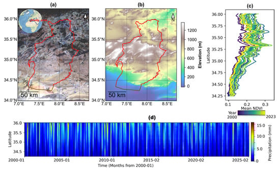
Figure 1.
Study area: Tebessa Province, Algeria. (a) Satellite image; (b) DEM; (c) mean NDVI by Latitude from 2001 to 2023; (d) Hovmöller plot of daily precipitation.
Land cover (LC) transitions were recorded from the year 2001 to 2022 in Tebessa Province, reflecting significant decreases in vegetation cover, particularly croplands, grasslands, and shrublands, as shown in the comprehensive year-by-year bar diagram illustrated in Figure 2a. This trend aligns with broader regional findings showing rapid vegetation degradation due to climate variability and anthropogenic pressures [28,29,30,31,32]. Concurrently, barren land exhibits a notable increase, reflecting the effects of desertification processes driven by prolonged droughts, overgrazing, and unsustainable land-use [28,29,30,33]. Figure 2b, a detailed Land-Use and Land-Cover (LULC) classification map for the year 2022, spatially reinforces these observations. Croplands, represented by deep red areas, have substantially declined, with a concentration predominantly in the northern and central parts, while barren areas dominate the southern regions. These transformations emphasize escalating environmental degradation risks, highlighting the urgent need for sustainable land management interventions [10,24,25,26,27,34].
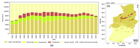
Figure 2.
Land cover dynamics and transitions in Tebessa Province, Tebessa, Algeria (2001–2022); (a) time series bar plot; (b) land-use map for 2022.
2.2. Data and Preprocessing
The data utilized in this study encompass diverse thematic categories, including vegetation properties, weather parameters, soil characteristics, and indicators of human activities. The dataset used in this study is presented in Table 1. Data acquisition leverages integrated geospatial datasets consistent with methodologies previously established for land degradation analyses [28,29,30,31,32,33]. Preprocessing steps include normalization, resampling, and spatial clipping, ensuring standardized and consistent inputs for model compatibility and effective geospatial analysis [31,32,34,35,36,37,38,39].

Table 1.
Datasets utilized in this study.
2.3. Methodology
2.3.1. Integrated Workflow Architecture for Desertification Prediction
Our workflow integrates satellite-derived geospatial inputs, ecological indices from the MEDALUS framework, and multiple AI modeling architectures to generate reliable spatial predictions of land degradation. Figure 3 presents a Sankey diagram that visualizes the full methodological pipeline employed in this study for predicting DSI.
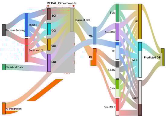
Figure 3.
Integrated workflow architecture for desertification prediction.
The workflow begins with two primary data streams: remote sensing (MODIS and Sentinel-1/-2) and statistical data (e.g., population density, land-use, etc.). These inputs feed into the computation of the four core MEDALUS indices—CQI, SQI, VQI, and LQI—after undergoing normalization and aggregation. Each of these indices captures a critical dimension of environmental sensitivity and contributes to calculating the Current DSI, which serves as both a mapping output and a ground truth for model training.
Subsequently, the Current DSI is used to train two categories of models: machine learning (ML) and deep learning (DL). ML models include SVM, XGBoost, and RF. DL architectures include LSTM, CNN, and DeepMLP. These models were selected for their complementary capabilities: RF and XGBoost handle nonlinear feature interactions effectively, CNNs exploit spatial textures from high-resolution data, and LSTM captures temporal dependencies critical for modeling degradation trends.
The performance of each model is evaluated using standard metrics: coefficient of determination (R2), root mean square error (RMSE), and mean absolute error (MAE). These metrics help quantify how well each algorithm can generalize from training data to accurately predict the final Predicted DSI across unseen spatial and temporal domains.
Notably, this diagram also highlights the role of AI Integration as a parallel driver, influencing both data processing and modeling choices. The inclusion of deep learning in particular enables the system to learn complex spatiotemporal relationships that classical methods cannot easily capture.
Overall, this integrated pipeline merges physical indices, statistical indicators, and machine/deep learning models into a unified system, providing a scalable and interpretable framework for desertification assessment at regional scales.
2.3.2. MEDALUS Model
The MEDALUS model was initially designed to assess desertification sensitivity specifically within Mediterranean-type ecosystems. Its structure is well aligned with the climatic and land-use conditions typical of such regions, which are characterized by hot, dry summers, cooler wet winters, and high interannual variability in rainfall. Additionally, the Mediterranean landscape is marked by complex anthropogenic and naturogenic pressures. These pressures can be addressed through a factor-based approach that integrates climate (CQI), soil (SQI), vegetation (VQI), and land-use (LQI) components, effectively capturing the biophysical dynamics of Mediterranean ecosystems [24]. The model’s simplicity—achieved through the use of normalized indicators and geometric mean aggregation—also facilitates its integration into remote sensing and Geographic Information System (GIS) platforms, making it an efficient tool for spatial analysis in the heterogeneous Mediterranean landscape.
As mentioned earlier, the MEDALUS framework employs two key mathematical techniques—normalization and geometric mean aggregation—to synthesize multi-dimensional environmental data into meaningful quality indices. First, normalization is used to standardize diverse variables, such as precipitation, soil organic carbon, or vegetation indices, by converting them to a common, dimensionless scale—typically ranging between 0 and 1. This standardization ensures that each indicator contributes objectively to the composite index, regardless of its unit, range, or data source. This is particularly valuable when integrating variables derived from heterogeneous platforms such as satellite remote sensing and field surveys. Second, the geometric mean is applied to aggregate these normalized indicators into single indices (e.g., CQI or DSI). Unlike the arithmetic mean, the geometric mean is especially sensitive to low values, thereby reflecting the “limiting factor” principle: a single poorly performing environmental component (e.g., highly degraded soil) can disproportionately affect the overall desertification risk score. This makes the method ecologically meaningful, as it aligns with the idea that land degradation is often driven by the weakest link in the ecosystem. For example, the CQI is calculated as the geometric mean of six normalized climatic sub-indicators, ensuring that vulnerability is not underestimated if one of them indicates extreme stress.
In its original formulation, the MEDALUS model assigns equal weight to each sub-indicator within its component indices. This decision is grounded in the model’s guiding philosophy of transparency and simplicity, facilitating widespread replicability across Mediterranean-type regions. Equal weighting avoids the need for subjective judgment or expert calibration, making the model accessible and enabling consistent cross-study comparisons. Conceptually, this reflects an assumption that all major environmental factors—climate, soil, vegetation, and land management—contribute equally to land degradation risk under typical conditions. The four main MEDALUS indices are presented below.
- Soil Quality Index (SQI)
SQI is a key indicator in the MEDALUS Model used to assess the overall health, fertility, stability, and resilience of soil in a given area. SQI evaluates how well the soil is capable of supporting vegetation, retaining moisture, preventing erosion, and resisting desertification. SQI combines four primary sub-indicators (soil texture, soil depth, organic matter, soil moisture) that are critical for assessing soil health, as shown in Equation (1).
where ST is the soil texture, SP is the soil depth, OM is the organic matter, and SM is the soil moisture.
SQI = (ST × SP × OM × SM)1/4
- Climate Quality Index (CQI)
CQI is an important composite indicator used to assess the impact of climate conditions on desertification risk and land degradation. It integrates multiple climate-related factors that influence soil and vegetation health, such as precipitation, temperature, aridity index, and wind speed, as shown in Equation (2).
where P is the precipitation, T is the temperature, AI is the aridity index, and WS is the wind speed.
- Vegetation Quality Index (VQI)
VQI is a composite indicator in the MEDALUS model that assesses the health, stability, density, and coverage of vegetation in a given area. It is used to monitor and evaluate the effectiveness of vegetation in preventing soil degradation and desertification. VQI combines multiple indicators that reflect the quality of vegetation cover, such as NDVI, vegetation cover, and vegetation density, as shown in Equation (3).
where NDVI is the Normalized Difference Vegetation Index, VC is the vegetation cover, and VD is the vegetation density.
- Land Management Quality Index (LQI)
LQI is a composite indicator used to assess the role of land cover and human activities in desertification process. The LCI incorporates three sub-indicators, which are land-use classification, human population density, and economic activity intensity, as shown in Equation (4).
where LC is the land-use classification, HPD is the human population density, and EA is the economic activity.
- Desertification Sensitive Index (DSI)
DSI is a comprehensive metric used to assess the vulnerability of land to desertification, which is the process of land degradation in arid, semi-arid, and dry sub-humid areas primarily due to climatic variations and human activities. This index incorporates multiple environmental factors to evaluate how susceptible a given area is to desertification. The Geometric Mean Method, shown as Formula (5), combines the indicators multiplicatively, allowing for an interaction effect between the variables, and assuming a complementary, interdependent, and synergistic interaction in influencing desertification risk:
Equal weight (via the 4th root) implies that all four indicators are considered equally critical to desertification risk. This means that a low value in one index will have a greater dampening effect on the final result, reflecting the reality that desertification can be driven by weaknesses in any single factor.
DSI values are classified into categories reflecting the degree of sensitivity to desertification. A high DSI indicates significant risk, meaning the land is highly susceptible to degradation—common in regions with poor soil, sparse vegetation, extreme temperatures, low rainfall, and high evaporation. Such areas are prone to becoming arid or semi-arid, resulting in decreased agricultural productivity, biodiversity loss, and desert expansion. Conversely, a low DSI signifies areas more resistant to desertification. These regions often have healthy soils, sufficient vegetation, and favorable climates, including stable precipitation and moderate temperatures. Such conditions support land stability and productivity, making these areas better suited for sustainable land management. Table 2 shows the standard classification for DSI (Geometric Mean Method) [40,41,42].
Table 2.
DSI Standard classification (Geometric Mean Method).
MEDALUS indicators (CQI, SQI, VQI, and LQI) follow the same standard classification as DSI in terms of range and classification: divided into five levels, ranging from 0 to 1 and from very low to very high, respectively); but they are inverse to DSI in terms of risk interpretation and description, where a higher value indicates higher risk for DSI, whereas for these indicators, a higher value corresponds to lower risk, with the same five-level descriptive scale applied in reverse.
2.3.3. Machine and Deep Learning Models
Predictive modeling incorporates several advanced deep learning and machine learning techniques, including LSTM, CNN, MLP, XGBoost, RF, and SVM, each recognized for effectiveness in environmental modeling and land cover classification [43,44,45]. Iterative evaluations, parameter optimization, and performance validations ensure robust model outcomes, ultimately generating precise Temporal–Spatial (TS) desertification risk maps.
The developed PyGEE-ST-MEDALUS model integrates remote sensing data within the MEDALUS framework, leveraging satellite-derived climate datasets and ground-level information. This integrated approach aims to accurately assess current and future desertification vulnerabilities, providing critical insights for sustainable land management practices and resource allocation in environmentally sensitive areas [24]. Model training drew on 53 760 MODIS pixel-year samples with 30 predictors and 178 200 Sentinel-1/-2 pixel-year samples with 34 predictors. CNN and LSTM architectures processed input tensors of shape (3, 10, 1) temporal-window tensors, capturing spatial and temporal dependencies. In contrast, tree-based models like RF and XGBoost, as well as linear models like SVM and Multilayer Perceptrons (MLPs), operated on flattened feature vectors. The sample-to-feature ratios—approximately 1800:1 for MODIS and 5200:1 for Sentinel—are well above commonly recommended minimums, which often suggest at least 10:1 to 100:1, depending on model complexity. These ratios indicate a robust dataset, supporting effective training and ensuring a fair comparison between deep learning and classical machine learning models.
The comprehensive methodological workflow employed for assessing and predicting desertification risk in Tebessa Province (Algeria) is detailed in Figure 4. The initial stage comprises data acquisition across multiple thematic categories, including vegetation properties, weather parameters, soil characteristics, and human activity indicators, consistent with prior research utilizing integrated geospatial datasets for land degradation analysis [28,29,30,31,32,33]. Subsequent data preprocessing involves normalization, resampling, and spatial clipping to standardize input variables for compatibility and consistency within the model, following best practices for geospatial modeling in desertification contexts [40,46,47]. Data partitioning allocates 80% for training and 20% for validation purposes, in line with standard deep learning protocols.
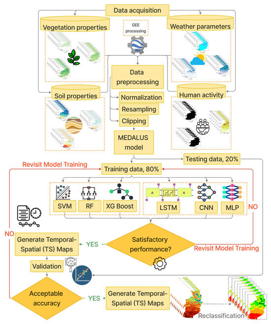
Figure 4.
Integrated workflow for desertification assessment using MEDALUS and machine and deep learning models.
The predictive modeling phase employs advanced deep and machine learning techniques, notably LSTM, CNN, MLP, XGBoost, SVM, and RF, all of which have demonstrated effectiveness in environmental modeling and land cover classification [10,48,49,50,51,52,53]. Models undergo iterative evaluation, parameter optimization, and performance validation until a satisfactory level of accuracy is achieved. Acceptable model performance enables predictions of Temporal–Spatial desertification risk maps. This rigorous methodological approach ensures high precision and reliability in assessing environmental degradation, providing critical insights necessary for effective land management and sustainable resource allocation in regions vulnerable to desertification [36]. The model architecture and parametrization are visible in Table A1.
To eliminate spatial and temporal leakage between calibration and evaluation, we adopted a two-tier blocking strategy. First, the entire hydrological year 2018 was withheld as an unseen temporal fold, providing a stringent test of inter-annual generalization. Second, the study domain was partitioned into non-overlapping 5 × 5 km tiles; tiles allocated to the training set were excluded from both validation and test folds. This combined leave-one-year-out and spatial-blocking protocol ensures that neighboring pixels or coincident years do not appear in multiple data partitions and therefore yields conservative, yet realistic, estimates of predictive skill.
The newly developed spatiotemporal assessment and prediction model, PyGEE-ST-MEDALUS, integrates remote sensing data with the MEDALUS framework and is implemented in combination with advanced machine and deep learning algorithms. This approach aims to identify current and future vulnerable areas and guide sustainable land management practices by leveraging satellite-derived climate datasets and ground-level information.
2.3.4. Training
To model desertification sensitivity across spatial and temporal dimensions, we implemented both deep learning and traditional machine learning approaches. Prior to model training, the dataset was partitioned into 80% for training and 20% for validation, consistent with standard deep learning protocols. The training subset (2001–2018) was used to fit the models, while the validation subset (2019–2022) supported hyperparameter tuning and overfitting control.
Deep learning models—including LSTM, CNN, and DeepMLP—were trained using the Adam optimizer with an initial learning rate of 0.001, reverting to 0.0005 if convergence stalled. Mean squared error (MSE) was employed as the loss function to minimize prediction error. Training was conducted over a maximum of 250 epochs, with early stopping applied if validation loss failed to improve for 10 consecutive epochs. This regularization strategy was especially critical for DeepMLP, which exhibited early signs of overfitting. Batch sizes were set at 32 for LSTM and 64 for CNN and MLP, and a dropout rate of 0.2 was introduced to enhance generalization. Hyperparameters—including learning rate, batch size, and dropout—were optimized via grid search. Evaluation on the MODIS dataset showed that CNN and LSTM achieved faster convergence and lower MSE (0.10–0.15), whereas MLP demonstrated slower convergence and a wider gap between training and validation loss. On the Sentinel dataset, models initially recorded higher errors (CNN ~0.60, LSTM ~0.90), but all converged toward an MSE of ~0.20 by around 200 epochs. CNN showed some fluctuation in validation loss, LSTM achieved smooth convergence, and MLP yielded the most stable loss curve overall.
Traditional machine learning models—RF, XGBoost, and SVM—were trained on the full training set using a batch learning approach. Hyperparameters were tuned using a combination of grid search and 5-fold cross-validation. For RF, the final model employed 100 trees with a maximum depth of 15, balancing model complexity and generalization. XGBoost was optimized with 100 boosting rounds, a learning rate of 0.1, a tree depth of 6, and a subsample fraction of 0.8 to encourage diversity among trees. Regularization parameters (L1 and L2) were kept at default moderate levels. For the RBF-kernel SVM, optimal performance was achieved with a penalty parameter C ≈ 10, a kernel width γ ≈ 0.1, and ε set to 0.01 for high prediction accuracy. Given the dataset’s scale, a stochastic approximation technique was applied to accelerate SVM training, which was terminated when improvements in loss fell below a defined threshold.
Overall, deep learning models—particularly CNN and LSTM—demonstrated superior capability in capturing the complex spatiotemporal patterns associated with desertification processes, outperforming MLP and the ensemble machine learning models across both MODIS and Sentinel datasets.
2.3.5. Validation
After training, each model was applied to predict DSI for the validation years 2019–2022 (for all spatial units), and the predictions were compared to the observed DSI (computed via MEDALUS for those years). We employ three metrics to quantitatively evaluate performance:
(I) Root Mean Square Error (RMSE): This is the square root of MSE, giving errors in the same units as the DSI. It penalizes larger errors more strongly, as shown in Equation (6).
(II) Mean Absolute Error (MAE): This measures the average magnitude of errors, giving equal weight to all deviations, as shown in Equation (7).
MAE is more interpretable in that it tells us, on average, how far predictions are from actual values (e.g., an MAE of 0.02 in DSI means the prediction is off by 0.02 DSI units on average).
(III) Coefficient of Determination (R2): This metric indicates the proportion of variance in the observed data that is explained by the model. It is computed as per Equation (8).
where is the mean of observed values. An R2 close to 1 implies the model’s predictions nearly perfectly align with actual values (it explains most of the variability), whereas R2 = 0 means the model is no better than predicting the mean, and negative R2 would indicate the model is worse than using the mean. We also report the Pearson correlation coefficient (R) between predicted and observed DSI as a complementary indicator of linear agreement. In our results, we found it useful to examine both R and R2: high correlation (R) indicates the model captures the ranking/relative changes in DSI well, while R2 reflects how correct the absolute values of the model are.
3. Results
3.1. MEDALUS Model Implementation and 2020-DSI Assessment
Figure 5 summarizes Tebessa’s desertification drivers after normalizing each MEDALUS component to a 0–1 scale following the scale and classification of the values into five ordinal risk classes (very low, low, moderate, high, very high) as per their standard classification already presented in Table 2. The reclassification of these values is also evaluated in different studies [46,47,48].
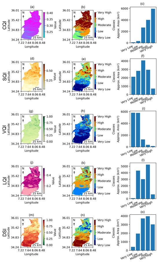
Figure 5.
MEDALUS model outputs and spatial classification of desertification indicators in Tebessa Province, Algeria (2020): (a) CQI; (b) CQI classification; (c) CQI class histogram; (d) SQI; (e) SQI classification; (f) SQI class histogram; (g) VQI; (h) VQI classification; (i) VQI class histogram; (j) LQI; (k) LQI classification; (l) LQI class histogram; (m) DSI; (n) DSI classification; (o) DSI class histogram.
CQI—panels (a–c). Panel (a) maps the 2020 CQI surface; panel (b) converts the continuous CQI into the five classes, and panel (c) reports the class areas. Roughly 6000 km2 (≈43%) fall in the high class (CQI ≥ 0.54), reflecting milder temperatures and higher rainfall, whereas ≈7000 km2 (≈50%) in the south register low to very low scores (CQI ≤ 0.30), signaling climatically driven vulnerability.
SQI—panels (d–f). Fertile, erosion-resistant soils dominate the north and center, with SQI > 0.62 (very high) over ≈7000 km2 (≈50%). Conversely, shallow, easily eroded soils (SQI < 0.30) occupy ≈3000 km2 (≈21%) in the southern plateau.
VQI—panels (g)–(i). Sparse or degraded vegetation (VQI < 0.30) covers ≈12,000 km2 (≈85%), leaving the landscape highly exposed to wind and water erosion. Dense, protective vegetation (VQI ≥ 0.62) is confined to just ≈2000 km2 (≈14%).
LQI—panels (j)–(l). Well-managed zones (LQI ≥ 0.54) account for ≈6000 km2 (≈43%), linked to sustainable cropping and controlled grazing. Poorly managed land (LQI ≤ 0.30) still represents ≈4000 km2 (≈29%), underscoring the importance of stewardship. Composite DSI—panels (m)–(o).
Integrating the four normalized indices reveals that more than 10,000 km2 (≈71%) of Tebessa now fall in the high to very high DSI classes (DSI ≥ 0.54). Only ≈2000 km2 (≈14%) remain in the low category (DSI < 0.30), primarily in well-managed northern highlands.
Overall, the normalized five-class analysis highlights extensive, multi-factor desertification pressure across Tebessa Province and reinforces the need for targeted interventions such as afforestation, soil-conservation measures, and improved land-management policies.
Spatial co-occurrence of low VQI, SQI, and LQI with high DSI suggests synergistic effects. In other words, this indicates the presence of a combination of poor soil, sparse vegetation, and bad management, leading to amplified degradation.
3.2. MODIS and Sentinel Datasets-Derived Correlation Matrices
Correlation matrices derived from MODIS (upper) and Sentinel (lower) datasets, incorporating original spectral bands, derived indices, and Principal Component Analyses (PCA) for 2020 are provided in Figure 6. The MODIS-derived correlation matrix illustrates strong negative correlations between DSI_2020 and spectral bands B1 through B7, with correlation coefficients ranging from −0.82 to −0.87, suggesting inverse relationships between spectral reflectance and desertification sensitivity. This implies healthier surfaces and lower desertification risk. Notably, PCA1 shows a robust positive correlation (0.87) with DSI, highlighting its significance in capturing variability related to desertification. Vegetation indices, including NDVI and EVI, exhibit a correlation that is not always opposite with DSI (0.75 and 0.70, respectively), implying that these areas are susceptible to stress, even if currently vegetated. Additionally, soil moisture (SOILM, 0.78) and evapotranspiration (ET, 0.80) show significant positive correlations, underscoring their critical roles. This may imply a temporal decoupling, suggesting that these same areas appear vegetated now but are very fragile and could degrade rapidly and considerably under environmental stress.
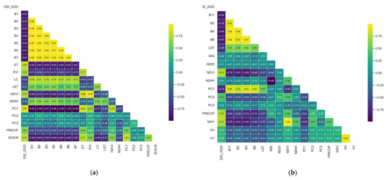
Figure 6.
Correlation matrices of environmental variables from (a) MODIS and (b) Sentinel data for Tebessa Province (2020).
The Sentinel-based matrix also identifies critical relationships; NDVI and Soil Adjusted Vegetation Index (SAVI) demonstrate strong positive correlations (0.75 each) with DSI (i.e., NDVI and SAVI showing consistent results as MODIS). On the other hand, precipitation also contains a good correlation with DSI and can be a potential dataset to be used in machine and deep learning analysis, emphasizing moisture’s protective role against desertification. Sentinel’s higher spatial resolution provides finer-scale detection of landscape variability, capturing microscale moisture and vegetation patterns relevant to degradation.
PCA components (PC1, PC2, PC3) present varying correlations, underscoring their differential capacities in explaining landscape variability relevant to desertification processes. They also highlight multivariate synergies not apparent in single indices—critical for deep learning feature selection.
3.3. Training and Validation Outcome
3.3.1. Training and Validations Behavior Along the Deep Learning Methods
Figure 7 illustrates the training and validation performance curves for three neural network models, CNN, DeepMLP, and LSTM, trained separately using MODIS and Sentinel-1/-2 datasets. When using MODIS data, the CNN exhibited rapid convergence, with both training and validation losses sharply decreasing within the initial 50 epochs. The mean squared error (MSE) declined from approximately 0.40 to about 0.10, stabilizing thereafter around this value by the 250th epoch. This rapid and stable convergence suggests effective model training with minimal signs of overfitting.
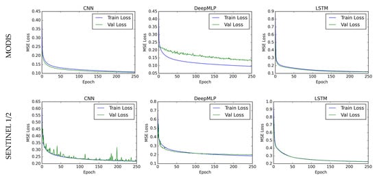
Figure 7.
Training and validations behavior along the deep learning methods.
In contrast, the DeepMLP showed slower convergence rates, with training loss gradually decreasing from around 0.35 to 0.10. However, the validation loss remained somewhat elevated at approximately 0.18, suggesting moderate overfitting due to reduced generalization to unseen data. The LSTM model demonstrated an initial rapid loss reduction similar to CNN, with a smooth and consistent convergence toward an MSE of about 0.15. Thus, both CNN and LSTM displayed superior convergence characteristics compared to DeepMLP for MODIS-derived data.
While stable convergence indicates efficient and stable model learning, it alone does not guarantee robust generalization. Robust generalization was explicitly confirmed through independent testing on unseen data and cross-validation metrics. Specifically, early convergence typically indicates rapid model learning efficiency but may also risk premature stabilization leading to underfitting. Conversely, delayed convergence may suggest thorough model learning but can potentially increase the risk of overfitting. Hence, evaluating convergence alongside validation metrics is critical to ensure the reliability and robustness of the models.
The second set of training and validation curves illustrates the performance of CNN, DeepMLP, and LSTM models trained on Sentinel-1/-2 data. CNN training showed initial fluctuations, with MSE losses quickly dropping from approximately 0.60 to near 0.20, stabilizing after 150 epochs, though intermittent spikes were evident in validation loss, indicating slight instability or noisy patterns in the validation dataset. The DeepMLP training presented a consistent reduction from about 0.70 to approximately 0.20, with validation loss closely aligned, reflecting effective generalization. Similarly, the LSTM model demonstrated a smooth convergence trajectory from a high initial loss (~0.90) to roughly 0.20 after 250 epochs, maintaining close alignment between training and validation losses, suggesting minimal overfitting and robust model performance. Notably, the Sentinel-based models experienced higher initial losses but achieved stable and comparable final performances across all three neural architectures.
In other words, CNN’s spatial pattern recognition is highly suited for spectral–spatial feature integration, ideal for desertification mapping. LSTM models excel in learning temporal dependencies (e.g., dry–wet season cycles, gradual degradation). While DeepMLP is effective but less robust to overfitting and complex spatiotemporal patterns.
3.3.2. Feature Importance Analysis for DSI Prediction Using MODIS and Sentinel Data
Figure 8 presents a comparative evaluation of feature importance for predicting DSI using two satellite datasets—MODIS (Figure 8a) and Sentinel (Figure 8b)—across six deep learning and machine learning models (CNN, DeepMLP, LSTM, RF, SVM, and XGBoost). In the MODIS-based analysis, soil moisture (SoilM) is the most influential predictor, with importance values peaking at 1.29 (RF), 1.23 (SVM), and 0.78 (DeepMLP). Land cover type (LC_Type1) is also highly important, with XGBoost assigning it a value of 1.31 and CNN 0.69. Spectral bands such as B4, B1, and B7 show intermediate contributions; for example, B4 reaches 0.31 in CNN and 0.20 in DeepMLP. The vegetation index NDVI remains consistently important, with a maximum value of 0.19 in RF and 0.17 in XGBoost. Thermal variables like LST_Night and LST_Day, as well as environmental metrics like evapotranspiration (ET) and precipitation, contribute modestly, ranging between 0.05 and 0.12.
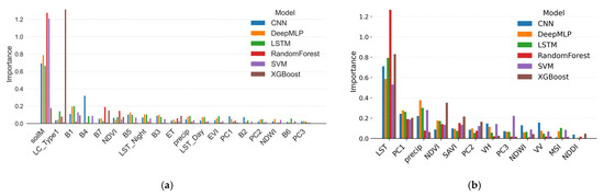
Figure 8.
Feature importance analysis for DSI prediction using (a) MODIS and (b) Sentinel data.
In contrast, the Sentinel-derived features highlight different key variables. Land surface temperature (LST) stands out as the most influential variable, with the RF model assigning it the highest importance (1.27), followed by XGBoost (0.83) and LSTM (0.79). CNN, DeepMLP, and SVM assign moderately high importance, ranging from 0.51 to 0.72. Other variables such as PC1 (0.22–0.28), precipitation (0.18–0.37), NDVI (up to 0.18), and SAVI (up to 0.15) also show moderate relevance. Meanwhile, features like PC2, VH, PC3, and NDWI register relatively low values, mostly under 0.20, while VV, MSI, and NDDI consistently remain below 0.10 across models.
The observed differences in feature importance between MODIS and Sentinel highlight not only the data source characteristics—MODIS being temporally rich and Sentinel offering finer spatial resolution—but also the inherent architectural preferences of the predictive models employed. For instance, CNNs are optimized for extracting spatial patterns, making them especially effective when paired with Sentinel’s high-resolution imagery and spectral indices (e.g., B4, NDVI, SAVI). CNNs leveraged localized spectral variation and edge patterns to discern land degradation patches, leading to strong performance where spatial texture is informative.
In contrast, LSTM models are designed to capture temporal dependencies, excelling in scenarios involving seasonal dynamics or gradual degradation. LSTM models benefited most from time-series predictors such as NDVI trends, evapotranspiration (ET), and land surface temperature (LST) from MODIS, which provided consistent longitudinal patterns that the model could learn over time. For example, LSTM effectively exploited MODIS-derived LST and ET because these variables exhibit cyclical or lagged relationships with vegetation stress, which LSTM can encode across time windows.
RF and XGBoost, being tree-based models, are highly effective at handling nonlinear relationships and variable interactions but lack intrinsic temporal or spatial encoding. These models performed well with strongly correlated features like soil moisture (SOILM), NDVI, and precipitation—especially in the MODIS dataset—because such features offered high individual predictive power. Their utility was enhanced by the models’ ability to rank splits and interactions without requiring structured input formats.
Deep Multilayer Perceptrons (DeepMLP) showed intermediate behavior, performing reasonably well when features were already pre-processed into meaningful representations (e.g., PCA components), but they were more prone to overfitting when faced with complex or noisy spatial-temporal signals. Their performance was enhanced when variables exhibited high linear correlation with DSI (e.g., NDVI, SOILM), but limited when variables required contextual interpretation over time or space.
Crucially, a feature’s importance is not determined solely by its direct correlation with DSI but also by how well the model architecture can exploit its structural characteristics. For example, NDVI may correlate moderately with DSI but becomes more useful in CNNs due to its spatial variability or in LSTM when tracked over time. Similarly, features like spectral band composites or principal components (e.g., PC1) are more effectively interpreted by RF and XGBoost, which excel at navigating multicollinearity and high-dimensional input.
These observations emphasize the model–feature alignment principle: predictive success depends not only on data quality but also on how well model architectures are matched to the intrinsic structure of the data. CNNs extract spatial meaning, LSTMs learn temporal dependencies, RF/XGBoost manage statistical heterogeneity, and DeepMLP requires clean, discriminative inputs. Thus, combining both MODIS and Sentinel datasets—and aligning them with diverse model types—offers a holistic, multi-resolution approach to modeling desertification risk, particularly in ecologically complex regions like Tebessa.
3.3.3. MODIS Dataset Versus Sentinel Dataset-Based Results
The performance of deep learning and machine learning trained on MODIS and Sentinel-1/-2 data for desertification mapping is presented in Figure 9, shows that CNN and RF models generally exhibit enhanced convergence behavior and robustness compared to DeepMLP, due to higher values of RMSE and MAE, with values like 0.03 and 0.022, respectively, that are the higher values between all methods for MODIS datasets. On the other hand, the SVM method has higher values of RMSE and MAE, with values of 0.04 and 0.03, respectively. These maximum values contrast with the values of the other methods, with a 0.005 difference.
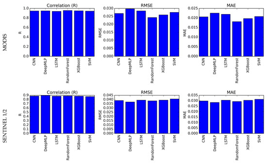
Figure 9.
MODIS dataset versus Sentinel dataset.
Key environmental variables influencing desertification sensitivity include Land Surface Temperature and Evapotranspiration for MODIS data, while the Normalized Difference Drought Index (NDDI) and principal components are crucial for Sentinel data. These findings highlight the importance of thermal and drought-sensitive indices in predicting desertification vulnerability.
3.4. DSI Annual Spatial Variations from 2001 to 2028
Annual spatial variations in the DSI classification in Tebessa Province over 28 years, from the year 2001 to 2028, are illustrated in Figure 10. The DSI maps for Tebessa from 2001 to 2028 present a clear trajectory of increasing desertification susceptibility, with alarming trends between 2020 and 2024, and projected beyond 2025. The general observation of spatiotemporal patterns is described by period (from 2001 to 2010, from 2011 to 2020, from 2020 to 2025, and beyond 2025) and region (northern and southern).
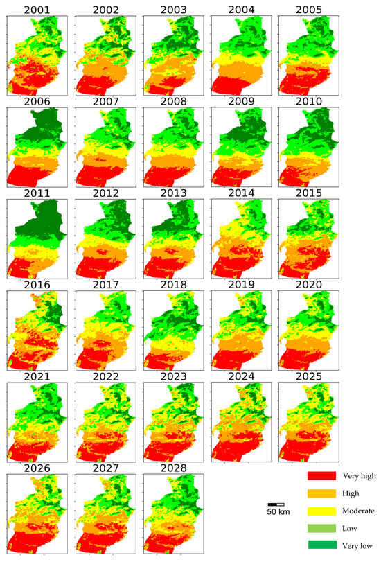
Figure 10.
The annual spatial distribution of DSI classified areas in Tebessa Province (2001–2028).
In the early period (2001–2008), DSI maps show stable conditions in the north (green), indicating low desertification risk, while the south remains highly vulnerable (orange to red), forming a persistent north–south gradient with minimal interannual variation. Between 2009 and 2013, the transition zone begins to shift, with yellow-green areas turning orange to red—particularly in central regions—i.e., increased pressures due to land-use and climatic stress.
From 2015 to 2024, vulnerability intensifies. Orange-red zones expand northward, and green zones contract, particularly between 2022 and 2024. Central and southern regions display widespread susceptibility, reflecting mounting environmental stress. Although certain years (e.g., 2017 and 2023) show brief recoveries in the north, the overarching trend indicates advancing land degradation and diminishing ecological buffers—underscoring the urgency for intervention. Without mitigation, these trends may accelerate, exacerbating the loss of fertile land and increasing socio-economic instability. Targeted policies and sustainable land management strategies are now essential to halt and reverse the degradation trajectory. From 2025 to 2028 (projections), a significant intensification of desertification risk is projected. By 2028, much of Tebessa, especially central and southern parts, will fall into the “high” and “very high” risk categories. The north remains relatively stable, but with pockets of moderate susceptibility.
3.5. Extrapolation with SARIMA
Seasonal Auto-Regressive Integrated Moving Average (SARIMA) [49,50] was employed to extrapolate DSI trends for the 2025–2028 period, using historical observations from 2001 to 2024, as shown in Figure 11. SARIMA effectively captured seasonal and interannual variability, revealing a continuous rise in desertification risk, particularly in southern Tebessa. In 2025, a strong north–south gradient appears, with low sensitivity in the north and very high in the south. By 2026, desertification worsens—high-risk zones expand, especially centrally, while low-sensitivity areas shrink. In 2027, degradation stabilizes, with some central areas shifting to moderate sensitivity, suggesting recovery or restoration. The year 2028 shows marginal improvement in central and northern zones, with a more balanced class distribution. Overall, the south remains at highest risk, highlighting the need for targeted intervention and adaptive land management. The consistent severity in southern Tebessa throughout the forecast period underlines the importance of sustained monitoring. Hence, integrating SARIMA outputs with socio-economic and land-use data could further refine intervention strategies and long-term resilience planning.
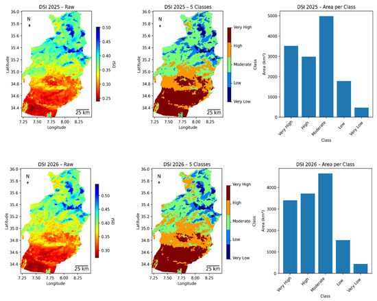
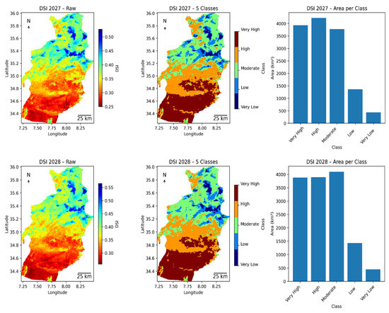
Figure 11.
Desertification Sensitivity Index (DSI) predictions from 2025 to 2028.
This approach was selected for its capacity to capture both seasonal and interannual variability in DSI dynamics. The model outputs revealed a persistent upward trend in desertification risk, particularly across the southern regions of Tebessa Province. To assess the reliability of the SARIMA model within this study’s framework, the full MODIS-derived DSI dataset was used to forecast values for 2023 and 2024. These predictions were then validated against independently derived DSI values from Sentinel-1/-2 data for the same years. The mean absolute error (MAE) was calculated to quantify prediction accuracy, and the resulting error values are presented in Figure 12, highlighting the model’s performance across both years.
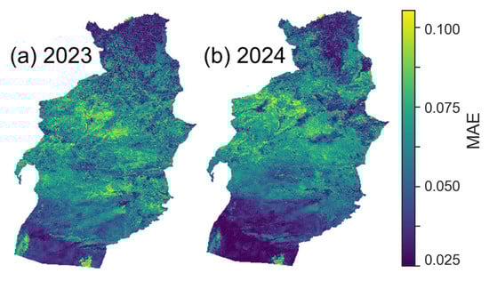
Figure 12.
Mean absolute error (MAE) of DSI predictions for 2023–2024 (a and b, respectively), generated using SARIMA forecasting models trained on the MODIS dataset (2021–2022), and compared against DSI predictions derived from Sentinel-1/-2 data for the same period.
3.6. DSI Annual Trends and Spatial Distribution from 2001 to 2028
An extensive analysis of temporal and spatial patterns in desertification sensitivity areas is provided in Figure 13, categorized from “very low” to “very high” risks for the 2001–2028 period. Panel (a) illustrates the overall study area (~12,500 km2), showing a progressive increase in high-risk desertification categories (“high” and “very high”), from approximately 4500 km2 in 2001 to nearly 7500 km2 by 2028, reflecting pronounced vegetation degradation and climate-driven stress. Simultaneously, “very low” and “low” classes (green and light green) show a sharp reduction, indicating a shift toward land degradation. Around 2020 marks a tipping point where medium and high sensitivity areas dominate. This trend aligns well with broader climate projections for North Africa, emphasizing intensified droughts, land-use stress, and vegetation loss.
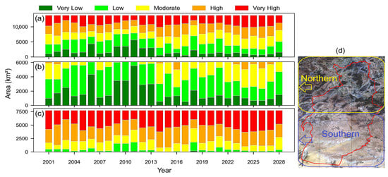
Figure 13.
Annual trends and spatial distribution of desertification sensitivity area (km2) from 2001 to 2028 for (a) entire study area, (b) northern area, and (c) southern area; (d) geographic division of the study region.
Panel (b) for the northern sub-region (~6000 km2) demonstrates predominantly moderate-to-low desertification sensitivity (~2500–4000 km2 in lower-risk categories), but a gradual increase in moderate and high categories from 2015 onwards indicates deteriorating vegetation conditions. This reflects partial ecological resilience, likely due to higher rainfall, vegetative cover (steppe and forest), lesser anthropogenic pressure compared to the south. Panel (c) highlights the southern region (~7500 km2), consistently displaying severe desertification sensitivity, dominated by “high” and “very high” categories, reaching up to 6500 km2, emphasizing severe vegetation loss and environmental fragility. The likely causes are arid climate and shallow soils, overgrazing and intensive agriculture, limited vegetation recovery after droughts, higher exposure to wind, and water erosion.
3.7. MODIS Versus Sentinel Dataset-Based Predictive Performance
For the MODIS dataset, shown in Figure 14 and Figure 15, the predictive accuracy of all models noticeably improved. RF emerged as the strongest model, yielding an excellent correlation coefficient (R = 0.96), lowest RMSE (0.024), and lowest MAE (0.018). The CNN model also showed robust performance (R = 0.95, RMSE = 0.027, MAE = 0.021), closely followed by XGBoost (R = 0.95, RMSE = 0.026, MAE = 0.020). LSTM (R = 0.94) and SVM (R = 0.94) delivered slightly lower but impressive results, with RMSE around 0.028 and MAEs near 0.021. DeepMLP showed comparable correlation (R = 0.95) but slightly higher RMSE (0.030) and MAE (0.023). The linear regressions indicated slopes closer to unity than Sentinel data, ranging between 0.75 (DeepMLP) and 0.90 (RF), highlighting that model trained on MODIS data yielded less biased predictions and superior alignment with observed DSI measurements. The DeepMLP model presented slightly lower performance, despite having R = 0.94, due to a higher RMSE (0.030) and MAE (0.023). All models displayed linear fits close to the 1:1 line, with slope values ranging from 0.77 (DeepMLP) to 0.89 (RF, XGBoost), indicating minor systematic biases in predictions.
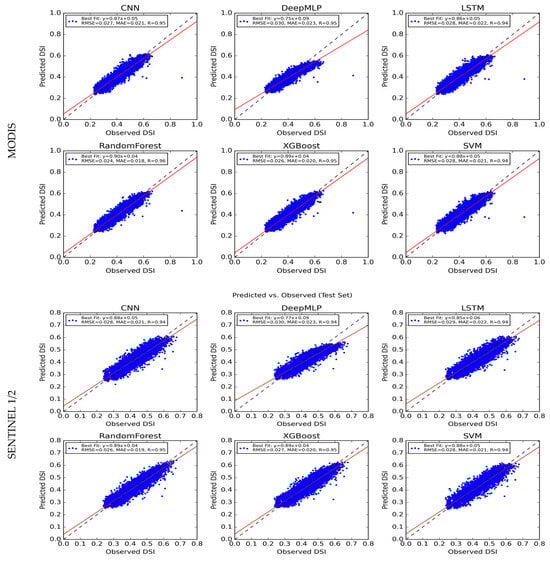
Figure 14.
Predicted versus observed MODIS and Sentinel-based dataset using CNN, DeepMLP, and LSTM.
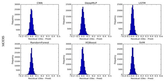
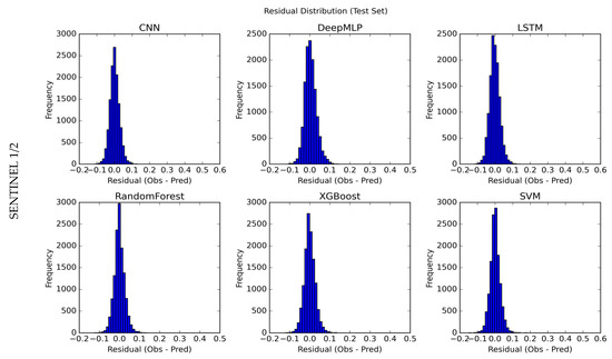
Figure 15.
Frequency versus residual MODIS and Sentinel-based dataset using CNN, DeepMLP, and LSTM.
Figure 15 illustrates the residual distributions—defined as the difference between observed DSI and predicted DSI—for six machine learning models (CNN, DeepMLP, LSTM, RF, XGBoost, and SVM). The top panel focuses on MODIS-based predictions, while the bottom panel displays those derived from Sentinel-1/-2 inputs. Each histogram plots residuals on the x-axis, spanning values from approximately −0.2 to +0.5, and the frequency of occurrences on the y-axis. Narrower histograms centered near zero typically indicate more accurate and unbiased predictions.
In the top (MODIS) set, RF, XGBoost, and CNN appear to have tightly clustered residuals with peaks around zero, suggesting robust predictions of DSI. DeepMLP and LSTM also show primarily small errors (concentrated between −0.1 and +0.1), though slightly more spread exists in the upper tail, implying the occasional overestimation of DSI. SVM exhibits a similar distribution pattern, albeit with a marginally wider spread. Overall, the bulk of residuals lie within a ±0.1 range, underscoring the suitability of MODIS data, combined with advanced machine learning, for capturing desertification dynamics.
In the bottom (Sentinel) set, the distributions follow a similar shape, yet some notable differences appear. Specifically, RF and XGBoost demonstrate even tighter residual clustering near zero, suggesting these models capitalize on the high spatial resolution and dual-sensor advantage (Sentinel-1 SAR and Sentinel-2 optical) to refine DSI predictions. CNN and LSTM also exhibit sharp central peaks, reflecting their capacity to extract meaningful spectral and textural features from Sentinel data. DeepMLP and SVM maintain distributions similar to the MODIS-based results, with minor deviations around ±0.1. The extended tails present in certain models (e.g., LSTM) indicate instances where complex environmental conditions may lead to under- or over-predictions.
Taken together, Figure 15 underscores the capacity of both MODIS and Sentinel data to support reliable DSI modeling, while highlighting how model architectures and input data sources influence residual distributions and, ultimately, predictive performance.
Though with slight biases in Sentinel data, the models demonstrated strong performance and robust predictive capabilities in estimating current and future desertification sensitivity.
4. Discussion
The spatial heterogeneity observed across Tebessa Province clearly reflected the complex interplay of climatic, topographic, and anthropogenic drivers of land degradation. This was consistent with the findings of Boali et al. (2024) and Yin et al. (2024), who demonstrated that desertification risks varied significantly with ecological context, particularly in arid and semi-arid landscapes [10,11].
In this study, the southern region, characterized by higher DSI values and temporal volatility, exhibited conditions resembling those of northeastern Iran and Central Asia, where Liu et al. (2025) and Meng et al. (2024) observed increased vulnerability linked to climate variability and land-use pressures [14,51]. The interannual variability in DSI, with spikes in 2004, 2006, and 2011, supported the non-static nature of desertification processes and aligned with the conclusions of Liu et al. (2024), who emphasized the importance of temporal monitoring using NDVI time-series data [16].
The post-2012 decline in median DSI values could have corresponded to favorable climatic phases or improved land stewardship, similar to the desertification reversals reported in some global drylands by Meng et al. (2024) [14]. Regionally, the northern Tebessa zone displayed lower and more stable DSI values, which was consistent with its cooler microclimate and higher vegetation productivity. This observation supported the work of Karimli and Selbesoğlu (2023), who found strong correlations between vegetation indices and land resilience, especially in temperate agroecological zones [12]. In contrast, the ecological fragility and DSI volatility in the south affirmed the hypothesis that minor perturbations in arid zones—such as overgrazing or rainfall anomalies—could trigger significant degradation, as reported by Boali et al. (2024) [10].
The utility of the MEDALUS framework in synthesizing biophysical parameters and land management indices (CQI, SQI, VQI, LQI) has been reaffirmed by multiple studies, including Boali et al. (2024) and Quang et al. (2022), who demonstrated its adaptability to diverse arid landscapes [10,17]. In this context, PCA proved effective for dimensionality reduction while preserving core variability, a technique also validated in large-scale applications such as Piao et al. (2021) [15]. Deep learning models—particularly LSTM and CNN architectures—outperform traditional machine learning algorithms in capturing the spatial and temporal dynamics of desertification. This finding aligns with Meng et al. (2024), who emphasized the power of interpretable machine learning (SHAP) in identifying nonlinear interactions, and Liu et al. (2025), who integrated probabilistic reasoning with spatial models for future risk projection [14,15,16,17,18,19,20,21,51]. To contextualize our approach within the recent literature, a structured comparison of related MEDALUS-based studies on desertification analysis is presented in Table 3. This table highlights the main data sources, modeling frameworks, and methodological advances across recent efforts, emphasizing their respective strengths and limitations. The comparative analysis demonstrates that while many previous studies applied the MEDALUS framework using either classical GIS or machine learning pipelines, our study distinguishes itself by integrating both spatiotemporal deep learning approaches and high-frequency MODIS and Sentinel observations over a two-decade period. Notably, few studies incorporated both climate and soil layers in a time-series predictive context, and even fewer studies leveraged explainable AI methods to address key interpretability gaps in predictive modeling.
Table 3.
Advantages and limitations-based comparative evaluation of previous studies with the current study in terms of core data and methods.
The superior performance of MODIS data over Sentinel-2 in long-term trend analysis could be attributed to MODIS’s temporal consistency and inclusion of thermal bands (e.g., LST), a feature noted by Guo et al. (2024) and Khan et al. (2024) as essential for detecting heat-driven vegetation stress [21,56]. By contrast, Sentinel-based models, while higher in spatial resolution, tended to underestimate extreme degradation cases, possibly due to their shorter temporal span and cloud-related gaps—limitations similarly observed by D’Acunto et al. (2024) [20].
To improve accuracy, future work should explore hybrid data fusion strategies combining MODIS and Sentinel-2, as suggested by Wang et al. (2024), and incorporate ancillary layers such as soil salinity, slope, and socioeconomic data [19]. These enhancements could improve model sensitivity in identifying emerging degradation hotspots. Moreover, incorporating explainable AI and Bayesian modeling, as performed by Liu et al. (2025), can help quantify uncertainty and enhance the interpretability of desertification models for policy use [51]. Lastly, real-time systems like the one proposed by Nathawat et al. (2025), powered by GEE and machine learning, offer promising tools for developing early warning systems in highly vulnerable southern zones of Tebessa [57].
5. Conclusions
This comprehensive assessment of desertification dynamics in Tebessa Province illustrated the robust capabilities of the PyGEE-ST-MEDALUS framework in capturing land degradation trends across local to regional scales. The key findings demonstrated that RF and CNN architectures achieved correlation coefficients (R) of up to 0.96 with MODIS-derived indices, reflecting strong agreement between predicted and observed desertification sensitivity. LSTM and DeepMLP models also performed well, with RMSE values below 0.03, underscoring the suitability of deep learning methods for environmental modeling.
Land surface temperature and evapotranspiration emerged as dominant predictors, each exhibiting correlations exceeding 0.80 with desertification indices. Additionally, the NDDI derived from Sentinel-2 data, along with principal components that integrated spectral and biophysical features, significantly enhanced model performance. Over 10,000 km2 (approximately 71% of the province) was classified as exhibiting “high” to “very high” desertification sensitivity. Spatiotemporal analyses revealed peak desertification years in 2004, 2006, and 2011, corresponding to prolonged drought episodes and heightened anthropogenic pressures. From 2012 onward, median DSI values showed a modest decline, potentially due to short-term climatic relief; nonetheless, the risk remains elevated in southern zones.
Notably, the province’s DSI distribution varies significantly between its northern and southern sectors. The northern region exhibits relatively stable and lower median DSI values, suggesting greater environmental resilience and possibly more effective land management practices. In contrast, the southern region displays higher temporal variability and elevated DSI values, indicative of increased vulnerability due to harsher climatic conditions and lower vegetation cover. This regional disparity underscores the importance of targeted, location-specific intervention strategies. Strong correlations (≥0.75) between vegetation indices—such as NDVI and Enhanced Vegetation Index (EVI)—and DSI revealed a dynamic interplay: as DSI intensified, drought-adapted vegetation types proliferated, while a reduction in DSI momentum did not necessarily correspond with ecological recovery, leaving vegetation still vulnerable to desertification. This finding highlights the complex feedback loop between desertification and vegetation resilience.
Finally, the seamless integration of Python-based deep learning algorithms with GEE’s cloud processing environment demonstrates broad applicability for data-scarce or climate-stressed regions. The flexibility to customize input variables, model architectures, and temporal resolution makes this approach a versatile and scalable tool for researchers and policymakers alike. In sum, PyGEE-ST-MEDALUS not only identifies regions at immediate risk but also anticipates future trends by integrating historical data spanning nearly three decades (2001–2028). The framework’s modular design and support for multi-source remote sensing data make it well-suited to guiding evidence-based environmental policies, including targeted reforestation, sustainable grazing practices, and optimized water resource allocation. With further refinements—such as higher-resolution imagery, improved SOILM retrievals, and real-time climate analytics—PyGEE-ST-MEDALUS can substantially advance global efforts to combat desertification and safeguard vulnerable dryland ecosystems.
Author Contributions
Conceptualization, Z.K.; methodology, Z.K. and I.G.; software, Z.K., F.P.A.L. and A.A.; validation, Z.K. and I.G.; formal analysis, Z.K. and F.P.A.L.; investigation, Z.K., F.P.A.L. and I.G.; resources, Z.K. and J.W.; data curation, F.P.A.L. and A.A.; writing—original draft preparation, Z.K., F.P.A.L. and I.G.; writing—review and editing, Z.K., F.P.A.L. and I.G.; visualization, I.G.; supervision, J.W. and G.Z. All authors have read and agreed to the published version of the manuscript.
Funding
This research received no external funding.
Data Availability Statement
The GEE repository for MEDALUS implemented by the authors is available in the following link: https://code.earthengine.google.com/8e4ee592e11bc6021bdfe158b793c5d5 (accessed on 31 May 2025).
Acknowledgments
The authors would like to thank the institutions and personnel who actively contributed and supported this research by providing the facilities and resources necessary for the successful completion of this work.
Conflicts of Interest
The authors declare no conflicts of interest.
Abbreviations
The following abbreviations are used in this manuscript:
| CMIP6 | Coupled Model Intercomparison Project Phase 6 |
| CNN | Convolutional Neural Network |
| CQI | Climate Quality Index |
| DeepMLP | Deep Multi-Layer Perceptron |
| DEM | Digital Elevation Model |
| DSI | Desertification Sensitivity Index |
| ET | Evapotranspiration |
| EVI | Enhanced Vegetation Index |
| GBM | Gradient Boosting Machine |
| GEE | Google Earth Engine |
| GLM | Generalized Linear Model |
| LC | Land Cover |
| LQI | Land Management Quality Index |
| LST | Land Surface Temperature |
| LSTM | Long Short-Term Memory |
| LULC | Land-Use and Land-Cover |
| MAE | Mean Absolute Error |
| MEDALUS | Mediterranean Desertification and Land Use |
| MLP | Multilayer Perceptron |
| MODIS | Moderate Resolution Imaging Spectroradiometer |
| MSAVI | Modified Soil-Adjusted Vegetation Index |
| MSE | Mean Squared Error |
| NDDI | Normalized Difference Drought Index |
| NDVI | Normalized Difference Vegetation Index |
| PCn | n Principal Component |
| PCA | Principal Component Analysis |
| PyGEE | Python Google Earth Engine |
| R | Correlation Coefficients |
| R2 | Coefficient of Determination |
| RF | Random Forest |
| rGEE | R for Google Earth Engine |
| RMSE | Root Mean Square Error |
| SARIMA | Seasonal Auto-Regressive Integrated Moving Average |
| SAVI | Soil Adjusted Vegetation Index |
| SHAP | SHapley Additive exPlanations |
| SOILM | Soil Moisture |
| SQI | Soil Quality Index |
| SVM | Support Vector Machine |
| TS | Temporal–Spatial |
| VQI | Vegetation Quality Index |
| XGBoost | eXtreme Gradient Boosting |
Appendix A
The appendix presents the architectures of all model used in this research.
Table A1.
Machine and deep learning models architecture.
Table A1.
Machine and deep learning models architecture.
| Model | Input Shape | Architecture Details | Parameters/Layers |
|---|---|---|---|
| CNN | (30,) | • Input reshaped to (3,10,1) • Conv2D: 32 filters, (2,2) kernel • Flatten • Dense(64) + ReLU • Dropout(20%) • Dense(1) linear | Filters: 32 Kernel: (2,2) Dense Units: 64 Dropout: 0.2 |
| DeepMLP | (30,) | • Dense(512) + ReLU • Dropout(30%) • Dense(256) + ReLU • Dropout(30%) • Dense(128) + ReLU • Dropout(20%) • Dense(64) + ReLU • Dense(1) linear | Dense Units: 512→256→128→64 Dropout Rates: 0.3→0.3→0.2 |
| LSTM | (3,10) | • LSTM(64) • Dropout(20%) • Dense(32) + ReLU • Dense(1) linear | LSTM Units: 64 Dense Units: 32 Dropout: 0.2 Return Sequences: False |
| RandomForest | (30,) | • 100 decision trees • Max tree depth: 15 | n_estimators: 100 max_depth: 15 random_state: 42 |
| XGBoost | (30,) | • Gradient boosted trees • 100 sequential trees • Max depth: 6 | n_estimators: 100 max_depth: 6 learning_rate: 0.1 |
| SVM | (30,) | • RBF kernel transformation • ε-insensitive loss | Kernel: rbf C: 1.0 epsilon: 0.1 |
References
- Berdyyev, A.; Al-Masnay, Y.A.; Juliev, M.; Abuduwaili, J. Desertification Monitoring Using Machine Learning Techniques with Multiple Indicators Derived from Sentinel-2 in Turkmenistan. Remote Sens. 2024, 16, 4525. [Google Scholar] [CrossRef]
- Jiang, Z.; Ni, X.; Xing, M. A Study on Spatial and Temporal Dynamic Changes of Desertification in Northern China from 2000 to 2020. Remote Sens. 2023, 15, 1368. [Google Scholar] [CrossRef]
- Habibie, M.I. The Application of Machine Learning using Google Earth Engine for Remote Sensing Analysis. J. Teknoinfo 2022, 16, 233. [Google Scholar] [CrossRef]
- Amani, M.; Ghorbanian, A.; Ahmadi, S.A.; Kakooei, M.; Moghimi, A.; Mirmazloumi, S.M.; Moghaddam, S.H.A.; Mahdavi, S.; Ghahremanloo, M.; Parsian, S.; et al. Google Earth Engine Cloud Computing Platform for Remote Sensing Big Data Applications: A Comprehensive Review. IEEE J. Sel. Top. Appl. Earth Obs. Remote Sens. 2020, 13, 5326–5350. [Google Scholar] [CrossRef]
- Antezana Lopez, F.P.; Zhou, G.; Jing, G.; Zhang, K.; Chen, L.; Chen, L.; Tan, Y. Global Daily Column Average CO2 at 0.1° × 0.1° Spatial Resolution Integrating OCO-3, GOSAT, CAMS with EOF and Deep Learning. Sci. Data 2025, 12, 268. [Google Scholar] [CrossRef]
- Ali, A.; Zhou, G.; Pablo Antezana Lopez, F.; Xu, C.; Jing, G.; Tan, Y. Deep learning for water quality multivariate assessment in inland water across China. Int. J. Appl. Earth Obs. Geoinf. 2024, 133, 104078. [Google Scholar] [CrossRef]
- Antezana Lopez, F.P.; Zhou, G.; Paye Vargas, L.; Jing, G.; Oscori Marca, M.E.; Villalobos Quispe, M.; Ticona, E.A.; Tonconi, N.M.M.; Apaza, E.O. Lithium quantification based on random forest with multi-source geoinformation in Coipasa salt flats, Bolivia. Int. J. Appl. Earth Obs. Geoinf. 2023, 117, 103184. [Google Scholar] [CrossRef]
- Shaik, A.S.; Shaik, N.; Priya, D.C.K. Predictive Modeling in Remote Sensing Using Machine Learning Algorithms. Int. J. Curr. Sci. Res. Rev. 2024, 7, 4116–4123. [Google Scholar] [CrossRef]
- Sellami, E.M.; Rhinane, H. Google Earth Engine and Machine Learning for Flash Flood Exposure Mapping—Case Study: Tetouan, Morocco. Geosciences 2024, 14, 152. [Google Scholar] [CrossRef]
- Boali, A.; Asgari, H.R.; Mohammadian Behbahani, A.; Salmanmahiny, A.; Naimi, B. Remotely sensed desertification modeling using ensemble of machine learning algorithms. Remote Sens. Appl. 2024, 34, 101149. [Google Scholar] [CrossRef]
- Yin, W.; Hu, Q.; Liu, J.; He, P.; Zhu, D.; Boali, A. Assessing Climate and Land-Use Change Scenarios on Future Desertification in Northeast Iran: A Data Mining and Google Earth Engine-Based Approach. Land 2024, 13, 1802. [Google Scholar] [CrossRef]
- Karimli, N.; Selbesoğlu, M.O. Remote Sensing-Based Yield Estimation of Winter Wheat Using Vegetation and Soil Indices in Jalilabad, Azerbaijan. ISPRS Int. J. Geoinf. 2023, 12, 124. [Google Scholar] [CrossRef]
- Gabriele, M.; Brumana, R. Monitoring Land Degradation Dynamics to Support Landscape Restoration Actions in Remote Areas of the Mediterranean Basin (Murcia Region, Spain). Sensors 2023, 23, 2947. [Google Scholar] [CrossRef]
- Meng, X.; Li, S.; Akhmadi, K.; He, P.; Dong, G. Trends, turning points, and driving forces of desertification in global arid land based on the segmental trend method and SHAP model. GIScience Remote Sens. 2024, 61, 2367806. [Google Scholar] [CrossRef]
- Piao, Y.; Jeong, S.; Park, S.; Lee, D. Analysis of Land Use and Land Cover Change Using Time-Series Data and Random Forest in North Korea. Remote Sens. 2021, 13, 3501. [Google Scholar] [CrossRef]
- Liu, Z.; Han, Y.; Zhu, R.; Qu, C.; Zhang, P.; Xu, Y.; Zhang, J.; Zhuang, L.; Wang, F.; Huang, F. Spatio-Temporal Land-Use/Cover Change Dynamics Using Spatiotemporal Data Fusion Model and Google Earth Engine in Jilin Province, China. Land 2024, 13, 924. [Google Scholar] [CrossRef]
- Vo Quang, A.; Delbart, N.; Jaffrain, G.; Pinet, C.; Moiret, A. Detection of degraded forests in Guinea, West Africa, based on Sentinel-2 time series by inclusion of moisture-related spectral indices and neighbourhood effect. Remote Sens. Environ. 2022, 281, 113230. [Google Scholar] [CrossRef]
- Lanfredi, M.; Coppola, R.; Simoniello, T.; Coluzzi, R.; D’Emilio, M.; Imbrenda, V.; Macchiato, M. Early Identification of Land Degradation Hotspots in Complex Bio-Geographic Regions. Remote Sens. 2015, 7, 8154–8179. [Google Scholar] [CrossRef]
- Wang, S.; Lv, K.; Ma, J.; Jiang, Q.; Ren, Y.; Gao, F.; Moazzam, N.S. A multi-source data fusion method to retrieve soil moisture dynamics and its influencing factors analysis in the ecological zone of the eastern margin of the Tibetan Plateau. Ecol. Indic. 2024, 169, 112877. [Google Scholar] [CrossRef]
- D’Acunto, F.; Marinello, F.; Pezzuolo, A. Rural Land Degradation Assessment through Remote Sensing: Current Technologies, Models, and Applications. Remote Sens. 2024, 16, 3059. [Google Scholar] [CrossRef]
- Anees, S.A.; Mehmood, K.; Rehman, A.; Rehman, N.U.; Muhammad, S.; Shahzad, F.; Hussain, K.; Luo, M.; Alarfaj, A.A.; Alharbi, S.A.; et al. Unveiling fractional vegetation cover dynamics: A spatiotemporal analysis using MODIS NDVI and machine learning. Environ. Sustain. Indic. 2024, 24, 100485. [Google Scholar] [CrossRef]
- Lei, X.; Liu, H.; Li, S.; Luo, Q.; Cheng, S.; Hu, G.; Wang, X.; Bai, W. Coupling coordination analysis of urbanization and ecological environment in Chengdu-Chongqing urban agglomeration. Ecol. Indic. 2024, 161, 111969. [Google Scholar] [CrossRef]
- Saharwardi, M.S.; Dasari, H.P.; Hassan, W.U.; Gandham, H.; Pathak, R.; Zampieri, M.; Ashok, K.; Hoteit, I. Projected increase in droughts over the Arabian Peninsula and associated uncertainties. Sci. Rep. 2025, 15, 1711. [Google Scholar] [CrossRef]
- Hossain, I.; Rana, M.d.S.; Haque, A.K.M.M.; Al Masud, A. Urban household adaptation to extreme heatwaves: Health impacts, socio-economic disparities and sustainable strategies in Rajshahi. Discov. Sustain. 2024, 5, 518. [Google Scholar] [CrossRef]
- Xin, X.; Liu, B.; Di, K.; Zhu, Z.; Zhao, Z.; Liu, J.; Yue, Z.; Zhang, G. Monitoring urban expansion using time series of night-time light data: A case study in Wuhan, China. Int. J. Remote Sens. 2017, 38, 6110–6128. [Google Scholar] [CrossRef]
- Cherif, I.; Kolintziki, E.; Alexandridis, T.K. Monitoring of Land Degradation in Greece and Tunisia Using Trends. Earth with a Focus on Cereal Croplands. Remote Sens. 2023, 15, 1766. [Google Scholar] [CrossRef]
- Weitkamp, T.; Jan Veldwisch, G.; Karimi, P.; de Fraiture, C. Mapping irrigated agriculture in fragmented landscapes of sub-Saharan Africa: An examination of algorithm and composite length effectiveness. Int. J. Appl. Earth Obs. Geoinf. 2023, 122, 103418. [Google Scholar] [CrossRef]
- Decha, R.; Adad, M.C. The City and its Spatial Transformations: A Diachronic and Quantitative Analysis of the Urban Sprawl Process. Case Study of Tebessa(Algeria). Int. J. Innov. Technol. Social Sci. 2024, 4, 1–15. [Google Scholar] [CrossRef]
- Macheroum, A.; Chenchouni, H. Short-term land degradation driven by livestock grazing does not affect soil properties in semiarid steppe rangelands. Front. Environ. Sci. 2022, 10, 846045. [Google Scholar] [CrossRef]
- Mihi, A.; Ghazela, R.; Wissal, D. Mapping potential desertification-prone areas in North-Eastern Algeria using logistic regression model, GIS, and remote sensing techniques. Environ. Earth Sci. 2022, 81, 385. [Google Scholar] [CrossRef]
- Feng, K.; Wang, T.; Liu, S.; Kang, W.; Chen, X.; Guo, Z.; Zhi, Y. Monitoring Desertification Using Machine-Learning Techniques with Multiple Indicators Derived from MODIS Images in Mu Us Sandy Land, China. Remote Sens. 2022, 14, 2663. [Google Scholar] [CrossRef]
- Zerrouki, N.; Dairi, A.; Harrou, F.; Zerrouki, Y.; Sun, Y. Efficient land desertification detection using a deep learning-driven generative adversarial network approach: A case study. Concurr. Comput. 2022, 34, e6604. [Google Scholar] [CrossRef]
- Kairis, O.; Karamanos, A.; Voloudakis, D.; Kapsomenakis, J.; Aratzioglou, C.; Zerefos, C.; Kosmas, C. Identifying Degraded and Sensitive to Desertification Agricultural Soils in Thessaly, Greece, under Simulated Future Climate Scenarios. Land 2022, 11, 395. [Google Scholar] [CrossRef]
- Borrelli, P.; Robinson, D.A.; Fleischer, L.R.; Lugato, E.; Ballabio, C.; Alewell, C.; Meusburger, K.; Modugno, S.; Schütt, B.; Ferro, V.; et al. An assessment of the global impact of 21st century land use change on soil erosion. Nat. Commun. 2017, 8, 2013. [Google Scholar] [CrossRef] [PubMed]
- Fentaw, A.E.; Yimer, A.A.; Zeleke, G.A. Monitoring spatio-temporal drought dynamics using multiple indices in the dry land of the upper Tekeze Basin, Ethiopia. Environ. Chall. 2023, 13, 100781. [Google Scholar] [CrossRef]
- Mpanyaro, Z.; Kalumba, A.M.; Zhou, L.; Afuye, G.A. Mapping and Assessing Riparian Vegetation Response to Drought along the Buffalo River Catchment in the Eastern Cape Province, South Africa. Climate 2024, 12, 7. [Google Scholar] [CrossRef]
- Zeng, Y.; Jia, L.; Menenti, M.; Jiang, M.; Barnieh, B.A.; Bennour, A.; Lv, Y. Changes in vegetation greenness related to climatic and non-climatic factors in the Sudano-Sahelian region. Reg. Environ. Chang. 2023, 23, 92. [Google Scholar] [CrossRef]
- Benhizia, R.; Phinzi, K.; Hateffard, F.; Aib, H.; Szabó, G. Drought Monitoring Using Moderate Resolution Imaging Spectroradiometer-Derived NDVI Anomalies in Northern Algeria from 2011 to 2022. Environments 2024, 11, 95. [Google Scholar] [CrossRef]
- Mahcer, I.; Baahmed, D.; Oudin, L.; Chemirik, C.H.K. Multidimensional analysis of NDVI dynamics in response to climate and land use/land cover change in Northwest Algeria. J. Hydrol. Hydromech. 2024, 72, 399–412. [Google Scholar] [CrossRef]
- Gad, A. Qualitative and Quantitative Assessment of Land Degradation and Desertification in Egypt Based on Satellite Remote Sensing: Urbanization, Salinization and Wind Erosion. In Environmental Remote Sensing in Egypt; Springer: Berlin/Heidelberg, Germany, 2020; pp. 443–497. [Google Scholar] [CrossRef]
- Chen, Y.; Ma, L.; Wang, X.; Liu, T.; Qiao, Z. Spatiotemporal patterns of desertification sensitivity and influencing factors across the Western Inner Mongolia Plateau, China. Ecol. Inform. 2025, 89, 103190. [Google Scholar] [CrossRef]
- Nguyen, B.T.; Dinh, G.D.; Le, L.B. Spatial and temporal-trend assessment of desertification-sensitive land using the desertification sensitivity index in the provincial Ninh Thuan, Vietnam. Environ. Monit. Assess. 2024, 196, 536. [Google Scholar] [CrossRef] [PubMed]
- Pradhan, B.; Dikshit, A.; Lee, S.; Kim, H. An explainable AI (XAI) model for landslide susceptibility modeling. Appl. Soft Comput. 2023, 142, 110324. [Google Scholar] [CrossRef]
- Xiao, Y.; Huang, M.; Xie, G.; Zhen, L. Evaluating the impacts of land use change on ecosystem service values under multiple scenarios in the Hunshandake region of China. Sci. Total Environ. 2022, 850, 158067. [Google Scholar] [CrossRef]
- Zhang, Y.; Liu, J.; Shen, W. A Review of Ensemble Learning Algorithms Used in Remote Sensing Applications. Appl. Sci. 2022, 12, 8654. [Google Scholar] [CrossRef]
- Han, X.; Jia, G.; Yang, G.; Wang, N.; Liu, F.; Chen, H.; Guo, X.; Yang, W.; Liu, J. Spatiotemporal dynamic evolution and driving factors of desertification in the Mu Us Sandy Land in 30 years. Sci. Rep. 2020, 10, 21734. [Google Scholar] [CrossRef]
- Bakr, N.; Weindorf, D.C.; Bahnassy, M.H.; El-Badawi, M.M. Multi-temporal assessment of land sensitivity to desertification in a fragile agro-ecosystem: Environmental indicators. Ecol. Indic. 2012, 15, 271–280. [Google Scholar] [CrossRef]
- Elnashar, A.; Zeng, H.; Wu, B.; Gebremicael, T.G.; Marie, K. Assessment of environmentally sensitive areas to desertification in the Blue Nile Basin driven by the MEDALUS-GEE framework. Sci. Total Environ. 2022, 815, 152925. [Google Scholar] [CrossRef]
- Kumari, S.; Muthulakshmi, P. SARIMA Model: An Efficient Machine Learning Technique for Weather Forecasting. Procedia Comput. Sci. 2024, 235, 656–670. [Google Scholar] [CrossRef]
- Martínez-Acosta, L.; Medrano-Barboza, J.P.; López-Ramos, Á.; Remolina López, J.F.; López-Lambraño, Á.A. SARIMA Approach to Generating Synthetic Monthly Rainfall in the Sinú River Watershed in Colombia. Atmosphere 2020, 11, 602. [Google Scholar] [CrossRef]
- Liu, J.; Ren, Y.; He, P.; Xiao, J. Quantifying Uncertainty in Projections of Desertification in Central Asia Using Bayesian Networks. Remote Sens. 2025, 17, 665. [Google Scholar] [CrossRef]
- de Jesus Macêdo, T.H.; Tagliaferre, C.; da Silva, B.L.; de Paula, A.; Lemos, O.L.; Adenilson Rocha, F.; Pinheiro, R.G.d.S.; Lima, A.C.S. Assessment of Land Desertification in the Brazilian East Atlantic Region Using the Medalus Model and Google Earth Engine. Land 2023, 13, 31. [Google Scholar] [CrossRef]
- Ogbue, C.; Igboeli, E.; Ajaero, C.; Ochege, F.U.; Yahaya, I.I.; Yeneayehu, F.; You, Y.; Wang, Y. Remote sensing analysis of desert sensitive areas using MEDALUS model and GIS in the Niger River Basin. Ecol. Indic. 2024, 158, 111404. [Google Scholar] [CrossRef]
- Nour-Eldin, H.; Shalaby, A.; Mohamed, R.M.; Youssef, E.; Rostom, N.G.; Khedr, H.S. Assessment of the desertification sensitivity of Northwestern El Minya Governorate, Egypt using MEDALUS model. Egypt. J. Remote Sens. Space Sci. 2023, 26, 758–767. [Google Scholar] [CrossRef]
- Hamad, K.O.; Surucu, A. Land degradation sensitivity and desertification risk in Harrir region, northern Iraq. Heliyon 2024, 10, e27123. [Google Scholar] [CrossRef]
- Guo, B.; Zhang, R.; Lu, M.; Xu, M.; Liu, P.; Wang, L. A New Large-Scale Monitoring Index of Desertification Based on Kernel Normalized Difference Vegetation Index and Feature Space Model. Remote Sens. 2024, 16, 1771. [Google Scholar] [CrossRef]
- Nathawat, R.; Singh, S.K.; Sajan, B.; Pareek, M.; Kanga, S.; Đurin, B.; Kantamaneni, K.; Rathnayake, U. Integrating Cloud-Based Geospatial Analysis for Understanding Spatio-Temporal Drought Dynamics and Microclimate Variability in Rajasthan: Implications for Urban Development Planning. J. Indian Soc. Remote Sens. 2025, 53, 1685–1704. [Google Scholar] [CrossRef]


Disclaimer/Publisher’s Note: The statements, opinions and data contained in all publications are solely those of the individual author(s) and contributor(s) and not of MDPI and/or the editor(s). MDPI and/or the editor(s) disclaim responsibility for any injury to people or property resulting from any ideas, methods, instructions or products referred to in the content. |
© 2025 by the authors. Licensee MDPI, Basel, Switzerland. This article is an open access article distributed under the terms and conditions of the Creative Commons Attribution (CC BY) license (https://creativecommons.org/licenses/by/4.0/).