Abstract
Bridge foundation settlement monitoring is crucial for infrastructure safety management, as uneven settlement can lead to stress redistribution, structural damage, and potentially catastrophic collapse. While traditional contact sensors provide reliable measurements, their deployment is labor-intensive and costly, especially for long-span bridges. Current remote sensing methods have not been thoroughly evaluated for their capability to detect and analyze complex foundation settlement patterns in challenging environments with multiple influencing factors. Here, we applied Small Baseline Subsets Synthetic Aperture Radar Interferometry (SBAS-InSAR) technology to monitor foundation settlement of a long-span bridge. Our analysis revealed distinct deformation patterns: uplift in the north bank approach bridge foundation and the left-side main bridge foundation (maximum rate: 36.97 mm/year), concurrent with subsidence in the right-side main bridge foundation and south bank approach bridge foundation (maximum rate: 35.59 mm/year). We then investigated the relationship between these settlement patterns and various environmental factors, including geological conditions, Sediment Transport Index (STI), Topographic Wetness Index (TWI), precipitation, and temperature. The observed settlement patterns were attributed to the combined effects of stratigraphic heterogeneity, dynamic hydrological conditions, and seasonal climate variations. These findings demonstrate that SBAS-InSAR technology can effectively capture complex bridge foundation deformation processes, offering a cost-effective alternative to traditional monitoring methods. This advancement in bridge monitoring technology could enable more widespread and frequent assessment of bridge foundation stability, ultimately improving infrastructure safety management.
1. Introduction
The design and construction of bridge foundations must fully consider various factors to ensure that the bridge maintains safety and functionality during long-term use. Bridge foundations not only bear the weight of the bridge’s own structure but also withstand external forces such as traffic loads, wind loads, and seismic loads, making them the most complex and difficult-to-construct part of the bridge structure [1,2,3,4]. Due to their complexity and importance, bridge foundation designs must carefully consider factors such as geological conditions, operating environment, and construction techniques [5,6,7]. In addition to meeting bearing capacity requirements under combined load conditions such as permanent, live, and environmental loads transmitted from the superstructure, the bridge foundation system should ensure sufficient overall stability and anti-overturning capability throughout its service life [8]. Even with strict ground treatment and foundation design methods, differential settlement remains a key technical issue that needs to be controlled in bridge foundation design due to factors such as heterogeneous stratigraphic conditions and uneven load distribution.
Uneven settlement refers to varying degrees of subsidence occurring in different foundation parts of a bridge due to various reasons, causing the bridge structure to bear additional stress and deformation [9]. This situation poses a potential threat to the bridge’s service life and safety. Multiple factors contribute to uneven settlement in bridge foundations. First, geological conditions are an important factor. The heterogeneity of soil types and conditions in the foundation is the most common cause [10,11,12]. In fact, each foundation location of a bridge often has unique soil characteristics, especially in areas with soft soils, fill soils, or significant fluctuations in groundwater levels, which are more prone to uneven settlement [13]. Another important factor is the complexity and uneven distribution of loads [14,15,16]. In practice, the traffic loads borne by bridges change frequently, and this unevenness is more pronounced on bridges with multiple lanes and heavy vehicle traffic [17]. Furthermore, changes in the external environment also significantly impact the settlement of bridge foundations. For example, variations in temperature and precipitation patterns caused by climate change can alter the moisture content of the foundation, thus affecting its bearing capacity [18]. Changes in groundwater levels, rain erosion, and river scouring may gradually reduce the strength of foundation materials, leading to settlement.
Due to these factors, bridge foundations are prone to uplift or settlement deformation. This situation may lead to bridge deck cracking, structural instability, tilting, or even irreversible damage, severely affecting bridge stability and driving safety [19]. Faced with the many causes of uneven settlement in bridge foundations, traditional detection techniques rely on observing and recording pavement conditions, making the investigation cumbersome and inefficient [20,21]. In fact, some periodic inspections and monitoring may have redundancies or fail to detect issues promptly, resulting in wasted efficiency and resources [22]. In contrast, using Interferometric Synthetic Aperture Radar (InSAR) technology to monitor surface and structural deformation can efficiently accomplish the important engineering task of bridge foundation settlement monitoring, ensuring the timely detection and handling of settlement issues, thereby guaranteeing bridge safety and stability [23].
InSAR is an advanced spatial measurement technology capable of obtaining continuous surface deformation information within a study area in a short period [24,25,26,27,28]. By analyzing reflected radar signals emitted from satellites or airplanes, InSAR can generate high-resolution surface deformation maps to monitor bridge settlement. A study by Lazecky et al. has shown that InSAR technology has broad application potential in bridge deformation monitoring [29]. In addition, Selvakumaran et al., combined InSAR datasets with traditional measurement techniques to enhance the accuracy of InSAR measurements [30]. InSAR technology has advantages such as a wide measurement range, no regional restrictions, and no impact on normal bridge operations [31,32,33,34,35,36]. These features make it particularly suitable for inaccessible or hazardous areas. It can monitor the overall deformation of bridges more quickly and comprehensively, making it highly applicable for bridge foundation settlement detection. For example, Selvakumaran et al., used the Tadcaster Bridge as a case study to demonstrate the application of InSAR in monitoring bridges at risk of scour [37]. Significant displacement changes were observed one month before the partial collapse of the bridge in 2015, indicating that InSAR can serve as an effective early warning system. Moreover, Guzman-Acevedo et al., evaluated the structural reliability of the Usumacinta Bridge in Mexico using InSAR technology [38]. Through probabilistic analysis of two and a half years of static displacement data, they derived the bridge’s reliability index and risk probability. The results showed that the bridge was undamaged under heavy load conditions, demonstrating that InSAR performs well in monitoring vertical displacements of bridges.
Time-series InSAR analysis methods have millimeter-level precision and are more suitable for long-term monitoring of bridge foundation settlement [39]. This method has been applied multiple times in bridge monitoring with good results. Studies have shown that Permanent Scatterer Synthetic Aperture Radar (PS-InSAR) technology has broad application potential in bridge settlement monitoring. For example, Zhao et al. explored the application of PS-InSAR in achieving high-precision settlement monitoring and timely detection of abnormal conditions [40]. Additionally, Lasri et al., used a concrete bridge in Isola Dovarese, Italy, as a case study [41]. They conducted PS-InSAR analysis using Sentinel-1 radar data and open-source software SNAP and StaMPS. By obtaining displacement time-series data, they quickly identified potential safety hazards in the bridge structure. The application of time-series InSAR analysis methods in bridge monitoring helps enhance infrastructure safety and emergency response capabilities. Ma et al. decomposed and geophysically interpreted the InSAR time-series deformation of the Hong Kong–Zhuhai–Macao Bridge using a synthetic aperture radar transformer [42]. Their proposed SAR-Transformer model was trained using synthesized InSAR time-series samples, reducing the mean absolute error by at least 58.32% and the mean absolute percentage error by at least 8.84%. This demonstrates the method’s effectiveness.
SBAS-InSAR technology calculates surface displacements in the vertical or horizontal direction by comparing SAR images acquired at different times and using their phase differences. Compared with traditional DS-InSAR technology, SBAS-InSAR can overcome limiting factors such as temporal and spatial decorrelation and atmospheric effects, providing more continuous and stable deformation information [43]. SBAS-InSAR reduces the impact of these factors by selecting image pairs with short temporal and spatial baselines for interferometric processing. This approach improves monitoring accuracy and reliability [44]. SBAS-InSAR technology has strong measurement capabilities and high precision. It can reduce the effects of temporal and spatial decorrelation and atmospheric delays [45]. This aids in exploring the correlation between different factors and deformation phenomena. It also helps in deeply understanding the intrinsic mechanisms of the deformation process [46]. Han et al. applied SBAS-InSAR technology to monitor surface deformation of the Pearl River Bridge in Nansha District, Guangzhou [47]. The results showed that SBAS-InSAR technology has significant advantages in nonlinear surface deformation monitoring. SBAS-InSAR is an effective tool for surface deformation monitoring, capable of monitoring dynamic deformation of bridges and providing reliable data support. Especially for foundation settlement monitoring of long-span bridges, this method offers higher spatial resolution and can accommodate changes in large monitoring areas. It considers atmospheric effects and performs reliable time-series analysis. For example, Zhou et al. used Sentinel-1A data and SBAS-InSAR technology to monitor the deformation of the Ganjiang Super Bridge and analyzed its deformation conditions and patterns [48]. They found that the internal deformation rate of the bridge ranged from 15.60 to 10.70 mm/year, with significant rebound deformation phenomena.
Although InSAR monitoring of bridge foundation settlement has advantages, relying solely on its measurement results cannot comprehensively account for the various influencing factors. To overcome this shortcoming, we innovatively propose a comprehensive analysis method based on SBAS-InSAR technology combined with other influencing factors. Specifically, we selected influencing factors closely related to bridge foundation deformation and analyzed the impact of each factor on bridge foundation settlement. This approach compensates for potential misconceptions that may arise from using InSAR detection alone.
This study is based on the aforementioned context and aims to conduct an in-depth analysis of the complex mechanisms underlying bridge foundation settlement through an innovative integrated analytical approach. This research will systematically integrate multidimensional influencing factors such as stratigraphic heterogeneity, dynamic hydrological environments, and seasonal climatic variations based on traditional InSAR monitoring. A comprehensive analytical model of bridge foundation deformation will be developed. This study will focus on the differentiated impacts of various factors on bridge foundation settlement. Combining quantitative analysis with qualitative interpretation, it seeks to comprehensively reveal the intrinsic patterns of bridge foundation deformation. By deeply integrating high-precision remote sensing deformation monitoring with multi-scale environmental factor analysis. This aims to provide more precise, systematic, and forward-looking technical solutions for bridge health assessments and risk warnings, thereby offering a scientific basis for the safe operation and maintenance management of bridge engineering.
2. Study Area and Data
2.1. Study Area
Huailai Bridge is located in Huailai County, Zhangjiakou City, Hebei Province, China. It spans the Guanting Reservoir and is an important part of the Shacheng–Donghuayuan Highway (see Figure 1). Known as the “First Span in North China”, Huailai Bridge has a total length of 1988 m and adopts a double-tower single-span suspension bridge structure. The main towers are 107.80 m high, and the main span stretches 720 m across the lake. The bridge is 33.60 m wide, designed to accommodate four lanes of urban arterial road traffic in both directions, with non-motorized vehicle lanes and sidewalks on both sides. The bridge is designed with a speed limit of 60 km/h, and its steel girders use advanced unpainted, environmentally friendly weathering steel [49]. The study area’s stratigraphy consists of Quaternary Holocene deposits, and the residual layers are mainly composed of sand, gravel, and silt. The pore water in loose rock formations has a double-layer structure; both the upper shallow water and the lower deep water yield 100–1000 m3/d per well.
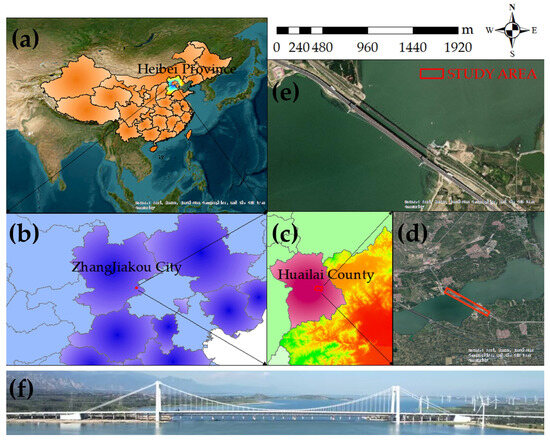
Figure 1.
Multi-scale visualization of Huailai Bridge: (a–e) satellite imagery at different scales; (f) ground-based photograph.
2.2. Datasets
This study utilized 20 Sentinel-1A images provided by the European Space Agency (ESA), spanning from July 2021 to March 2022, covering the study area. These images cover all areas of potential uneven foundation settlement that may affect the bridge’s safety, with acquisition intervals not exceeding one month. These images were acquired using the Interferometric Wide Swath (IW) mode with VV polarization. Detailed SAR data are provided in Table S1. In addition, this study used the 30 m Shuttle Radar Topography Mission (SRTM) Digital Elevation Model (DEM) from NASA to eliminate topographic phase effects. Simultaneously, precise orbit data (POD) released by ESA were used to refine orbital information and enhance georeferencing and baseline estimation accuracy. We also obtained geological borehole data around the bridge foundation from the Physical Geological Data Center of Natural Resources under the China Geological Survey to analyze the geological stratification of the study area. Furthermore, we employed daily dry bulb temperature and relative humidity data during the research period provided by the public resource EpwMap, jointly developed by the University of Pennsylvania and others. Detailed data are provided in Table 1.

Table 1.
Data sources for research analysis.
3. Methodology
This study analyzes the foundation settlement of a kilometer-scale bridge using SBAS-InSAR technology. By extracting key feature points of the bridge foundation and their time-series deformation data, we systematically evaluated the differential settlement characteristics of each connected part. Based on the SBAS-InSAR nonlinear deformation monitoring results, we explored the influence mechanisms of geological heterogeneity, hydrodynamic changes, and seasonal climate fluctuations on uneven foundation settlement. The research process is illustrated in Figure 2.
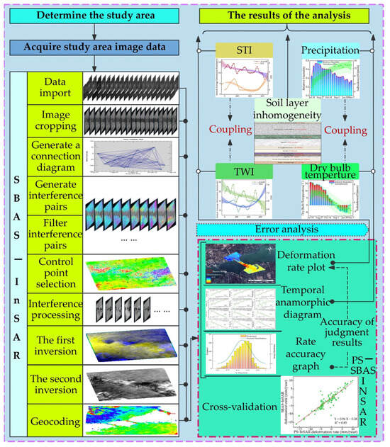
Figure 2.
Flowchart of the research.
3.1. Principle of SBAS-InSAR
The basic principles of SBAS-InSAR technology are as follows: SBAS-InSAR technology combines SAR image data into several subsets based on baseline thresholds, uses the deformation results obtained from single differences as observations, employs the least squares method to obtain high-precision deformation sequences for each subset, and utilizes singular value decomposition (SVD) to jointly solve multiple subsets, thereby obtaining the deformation sequence over the entire monitoring period. Suppose N + 1 images are acquired and arranged according to acquisition times t (t0, …, tN). Based on interferometric baseline combinations, M interferograms can be generated, and M satisfies the following inequality:
Assuming that interferogram j is generated by interfering the images acquired at times tA and tB (tB > tA), after removing flat-earth effects and topographic phase influences, the interferometric phase of a pixel located at range r and azimuth x in interferogram j can be expressed as follows:
In Equation (2), and are the phase values of the SAR images at times and , respectively; is the deformation phase in the radar line-of-sight direction from time to ; is the topographic phase error caused by inaccurate reference DEM; is the atmospheric phase error; and is the noise phase.
In Equation (3), A is an M × N coefficient matrix, where can be expressed as follows:
When the coefficient matrix B is full rank (i.e., M ≥ N), the deformation rate ν can be solved using the least squares method; when M < N, the matrix B becomes rank-deficient, and the deformation rate of the study area can be obtained using singular value decomposition (SVD) [50]. After obtaining the deformation rate, the deformation amount during the corresponding time intervals between SAR images in the study area can be calculated.
3.2. SBAS-InSAR Data Processing
Figure 3 illustrates the SBAS-InSAR processing flow.
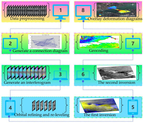
Figure 3.
Processing flow of SBAS-InSAR technology.
- (1)
- Generation of Interferometric Pairs: Automatically select the SAR image acquired on 10 July 2021 as the super master image. Using this master image as a reference, co-register and resample it with the other 19 SAR images separately to form N interferometric pairs. Each pair contains phase information of the same surface area at different times.
- (2)
- Interferometric Processing: Perform interferometric processing on each interferometric pair, including phase unwrapping and interferogram generation. The phase in the interferogram contains surface deformation information but is also affected by factors such as atmospheric delays and topographic fluctuations [51]. Statistical or physical models are used to estimate and correct atmospheric delays, reducing the impact of atmospheric effects on the interferometric phase.
- (3)
- Deformation Inversion: Use a robust linear model to invert surface deformation. Based on the acquisition of linear deformation of the surface, the Singular Value Decomposition (SVD) method is employed to derive the nonlinear deformation of the surface, and the linear deformation is added to the nonlinear deformation to obtain a comprehensive representation of the deformation information. During the first inversion, the displacement rate and residual topography are estimated. In the second inversion, based on the deformation rate from the first inversion, perform high-pass filtering in the temporal dimension and low-pass filtering in the spatial dimension to estimate and remove the atmospheric phase, thereby obtaining the final displacement results on a purer time series.
- (4)
- Geocoding: Geocode the SBAS-InSAR inversion results by converting the pixel coordinates of the SAR images into geographic coordinates (latitude and longitude) to facilitate analysis and interpretation. Remove outliers and interpolate the deformation results. The deformation produced by SBAS-InSAR is in the line-of-sight (LOS) direction.
3.3. Error Analysis of the Processing Procedure
To address phase measurement errors, the selected image dates for this study range from 10 July 2021 to 7 March 2022, with the Huailai Bridge having been put into operation on 28 June 2021. We assume that the image from 10 July 2021 did not undergo deformation during the observation period, and we extract terrain information from it to eliminate terrain effects, similar to the three-pass method. Unlike phase measurement errors, satellite orbit errors are systematic errors that present nearly identical discrepancies across all points within the measurement area and can be corrected using ground control points [52]. During the completion of the SBAS-InSAR process in the ENVI-Sarscape (version 5.3.1) software, ground control points are reselected during the interferometric processing to eliminate orbital errors [53,54]. Furthermore, the smaller the measurement area, the smaller the relative elevation error of ground points caused by satellite orbit errors. For smaller areas (e.g., with a measurement width of 5 km), even with a baseline error of approximately 1 m, a moderate effective baseline (e.g., 200 m) can still achieve high accuracy (approximately 16 m) [55]. To address phase unwrapping errors and improve the accuracy and reliability of deformation results, a manual selection method is employed to eliminate images with poor unwrapping results. Each image undergoes a visual inspection to observe the spatial distribution characteristics of the unwrapping results, allowing for the identification of images that exhibit anomalies either locally or globally, which are then excluded from the analysis. This step ensures that subsequent time series analysis and deformation inversion are based solely on high-quality unwrapped data, thereby reducing the impact of noise errors on the results.
3.4. The Topo-Hydrological Aspects
3.4.1. Topographic Wetness Index (TWI)
TWI is a physical indicator used to measure the influence of topography on runoff direction and water accumulation [56]. It is calculated based on the slope and the upstream catchment area. This index helps identify runoff patterns after rainfall, areas that may increase soil moisture, and the distribution of flooded regions.
In Equation (5), represents the slope, and SCA denotes the contributing area per unit width. SCA is obtained by the filling sinks in DEM data and then calculating the slope and flow direction. This study utilizes the ArcGIS platform for the computation of TWI. First, the DEM data are subjected to projection transformation to ensure that the units are in meters, thereby avoiding errors in slope calculation. Next, the DEM is filled to eliminate terrain errors, ensuring the accuracy of flow direction analysis. Subsequently, flow direction, contributing area, and slope are extracted, with particular attention paid to converting slope units from degrees to radians and addressing cases where the slope is zero. Finally, the TWI values are obtained through raster calculations.
3.4.2. Sediment Transport Index (STI)
STI is an indicator describing the sediment transport capacity of rivers within a watershed. It reflects the amount of sediment that rivers can transport over a certain period by evaluating various factors within the watershed, such as precipitation, soil type, topography, vegetation cover, and human activities.
In Equation (6), SCA and are the same as in the TWI formula; m is the contributing area exponent, usually set to 0.40; and n is the slope exponent, usually set to 1.40. The uniqueness of the STI calculation method lies in its comprehensive consideration of multiple dimensions of terrain; it not only focuses on the magnitude of slope but also emphasizes the hydrological characteristics of the upstream contributing area.
3.5. Statistical Methods
3.5.1. Time-Lagged Cross-Correlation (TLCC) and Windowed TLCC (WTLCC)
TLCC is a statistical method used to evaluate the correlation between two time series, specifically focusing on the relationship between one series and the lagged version of another [57]. This approach is particularly valuable in understanding the influence of one variable on another, especially when temporal delays are present [58]. The TLCC is calculated using the following formula:
where denotes the cross-correlation coefficient at lag ; and represent the values of the two time series; and and are their respective means.
WTLCC enhances the TLCC analysis by applying windowing techniques to mitigate boundary effects and improve the stability of the estimates [59]. Common windowing methods include the Hanning window, Hamming window, and rectangular window, which can be expressed mathematically as follows:
In this equation, is the window function applied to the original time series .
Utilizing windowed TLCC allows for more accurate analysis of relationships between time series, particularly in scenarios involving long datasets or high levels of noise [60]. Overall, TLCC and its windowed variant are essential tools for capturing dynamic relationships and understanding time delay effects within various fields such as economics, meteorology, and signal processing [61].
3.5.2. Variance Inflation Factor (VIF)
The VIF is an important statistical indicator for assessing the degree of multicollinearity [62]. In regression models, high correlation among independent variables may lead to inaccurate parameter estimates, increased variance, and diminished explanatory power of the model. The VIF quantifies the extent of linear dependence of one independent variable on others; a higher value indicates a stronger correlation with other independent variables, potentially leading to multicollinearity issues. For each independent variable , its VIF is calculated using the following formula:
where is the coefficient of determination obtained when is treated as the dependent variable and all other independent variables as predictors.
In regression analysis, examining the VIF values of independent variables helps identify potential multicollinearity issues, allowing for appropriate measures to be taken as needed, such as removing certain variables, performing variable selection, or applying alternative techniques (e.g., principal component analysis) to improve the model.
4. Result
4.1. Accuracy Verification
To ensure the accuracy of the processing results, we used Sarscape (version 5.2.1) software to process the Sentinel-1A SAR images and obtain an estimated average precision of velocity measurements, which was used to evaluate the processing accuracy. After vectorizing the SBAS processing results, we obtained estimation values for assessing the processing accuracy, namely, the estimated average precision of velocity measurements VPrecision and the fitting and inversion quality measure χ2. Specifically, a higher VPrecision indicates more precise velocity measurements, and a lower χ2 signifies better fitting and inversion quality. The obtained VPrecision and χ2 were first normalized using the formula:
In Equation (10), Z-score is the normalized result; Raster denotes the data to be normalized; Zmax is the maximum value; and Zmin is the minimum value. To enhance data reliability, we performed statistical calculations in Excel and plotted normal distribution graphs. We grouped all data with a step size of 0.05, counted the number of data points in each interval, and then drew a histogram. As shown in Figure 4, most selected points have VPrecision values between 0.15 and 0.8 and χ2 values between 0 and 0.3, indicating that the accuracy values are reliable.
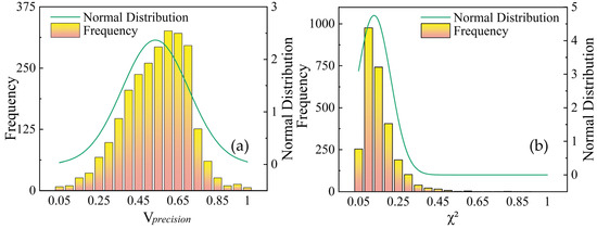
Figure 4.
Frequency distribution of InSAR measurements: (a) velocity precision histogram with normal distribution fit; (b) χ2 statistics for quality assessment.
Furthermore, a comparison was made between the results obtained using the SBAS-InSAR and PS-InSAR methods to validate the accuracy of the experiment. To more effectively validate the results of these two methods, 128 Permanent Scatterer (PS) points were randomly selected, and the correlation between the rates obtained from SBAS-InSAR and these points was analyzed. The results are shown in Figure 5. Figure 5a presents a statistical analysis of the deformation rate differences for 124 pairs of adjacent points. More than half of the adjacent points exhibited absolute differences within the range of 0 to 1 mm/year, with a mean and standard deviation of 1.35 mm/year and 0.66 mm/year, respectively, indicating a satisfactory comparison outcome. The deformation rate results from both methods are highly consistent. Figure 5b shows an value of 0.85 obtained through cross-validation, further indicating a good comparison outcome. Considering the differences in the random selection of PS points and the limitations of InSAR technology accuracy, there are slight discrepancies between the two methods. Therefore, it can be assumed that the deformation rate results obtained by both methods are similar in most areas.
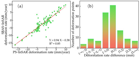
Figure 5.
(a) Cross-validation results. (b) Statistical analysis of deformation rates at random pseudo-steady points.
4.2. SBAS-InSAR Results
In this study, we used the SBAS-InSAR method to monitor the deformation rate of the bridge foundation within the study area. As shown in Figure 6, during the period from 10 July 2021 to 7 March 2022, the annual average deformation rate in the radar line LOS direction exhibited the following characteristics: the north bank mainly experienced ground uplift, while the south bank mainly experienced ground subsidence. The maximum foundation subsidence rate was 35.59 mm/year, and the maximum uplift rate was 36.97 mm/year. Areas with significant deformation were mainly concentrated in the bridge approach foundation areas. Additionally, the average coherence value of the 20 images was 0.54, with a maximum of 0.97 and a minimum of 0.004, indicating good overall image consistency.

Figure 6.
The spatial distribution of surface deformation rates derived from InSAR measurements along the radar LOS direction.
4.3. Time Series Cumulative Deformation
To further investigate the deformation of Huailai Bridge, we selected twelve characteristic points (P1–P12) along the bridge’s linear features to facilitate subsequent verification and analysis. The deformation rates and cumulative deformations of these points varied. The locations of these points are shown in Figure 7, and their time-series deformation graphs are presented in Figure 8. P1 is at the second pier of the north bank approach bridge, with an uplift rate of 20.28 mm/year and a cumulative uplift of 257.74 mm, considered a significant uplift point (all examples of cumulative deformation mentioned below refers to the total displacement accumulated across all time series). It is important to note that the LOS displacement refers to the displacement along the line of sight between the sensor and the target, while settlement and uplift are used solely for the purpose of describing and understanding the relative changes in these displacements [63]. P2 is at the sixth pier of the north bank approach bridge, with an uplift rate of 24.05 mm/year and a cumulative uplift of 289.18 mm, the point with the maximum uplift. P3 is at the tenth pier of the north bank approach bridge, with an uplift rate of 18.53 mm/year and a cumulative uplift of 217.22 mm, also a significant uplift point. P4 is on the left side of the main bridge near the anchorage, with an uplift rate of 18.22 mm/year and a cumulative uplift of 212.52 mm, a significant uplift point. P5 is on the left side of the main bridge near the pylon, with an uplift rate of 20.26 mm/year and a cumulative uplift of 248.38 mm, another significant uplift point. P6 is at the base of the left pylon of the main bridge, with an uplift rate of 11.30 mm/year but a cumulative subsidence of 199.74 mm, exhibiting complex deformation behavior. P7 is at the base of the right pylon of the main bridge, with a subsidence rate of 23.13 mm/year and a cumulative subsidence of 59.86 mm, a significant subsidence point. P8 is on the left side of the south bank approach bridge near the pylon, with a subsidence rate of 20.94 mm/year and a cumulative subsidence of 39.69 mm, another significant subsidence point. P9 is also on the left side of the south bank approach bridge, with a subsidence rate of 13.97 mm/year but a cumulative uplift of 8.57 mm, exhibiting slight uplift. P10, P11, and P12 are on the south bank approach bridge, with subsidence rates of 14.75 mm/year, 14.50 mm/year, and 14.71 mm/year, and cumulative subsidence amounts of 4.14 mm, 27.60 mm, and 41.39 mm, respectively, all being slight subsidence points.

Figure 7.
Distribution of structural monitoring points: (upper) reference points P1 and P12 at 30 m from bridgeheads, with measurement points P2–P11 at 120 m intervals along bridge span; (lower) detailed view of monitoring points at bridge foundation.
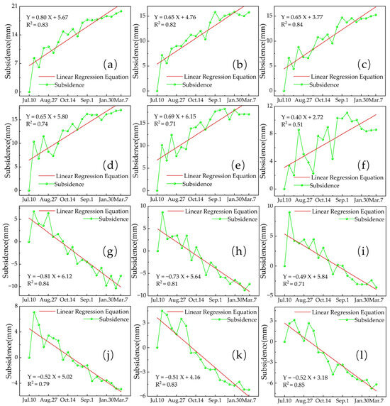
Figure 8.
Time-series deformation maps of monitoring points P1–P12. Subplots (a–l) illustrate cumulative displacement trends, where dotted lines represent measured settlement values and solid lines denote linear regression fits with corresponding equations.
Based on the results, the cumulative deformation of monitoring points P1–P12 during the study period is as follows. The north bank approach bridge (P1–P3) and the left side of the main bridge (P4–P5) exhibit significant uplift trends, with the maximum cumulative uplift reaching 289.18 mm at P2. In contrast, the right side of the main bridge (P6–P7) and the south bank approach bridge (P8–P12) mainly show subsidence trends, with the maximum cumulative subsidence reaching 199.74 mm at P6. Notably, some monitoring points show inconsistencies between the annual deformation rate and the cumulative deformation, such as P6 and P9. This may indicate that the bridge experienced complex deformation processes during the study period. In particular, significant deformation occurred at the base of the right pylon of the main bridge (P6–P7), indirectly indicating that substantial structural adjustments might have occurred in that area.
The results show that the foundation of Huailai Bridge experienced uneven deformation during the study period. The foundation of the north bank approach bridge and the left side of the main bridge generally showed uplift trends, while the foundation of the right side of the main bridge and the south bank approach bridge tended to subside. This complex deformation pattern requires further analysis of its causes and continuous monitoring to ensure the bridge’s long-term safety and stability.
4.4. Deformation Patterns Surrounding Bridge Foundations
This study expands the analysis of the surrounding areas of the bridge to gain a more comprehensive understanding of the relationship between ground deformation and bridge displacement. By collecting and processing annual average deformation rate data from points located 10 m on either side of the bridge deck, perpendicular to the bridge axis, it was found that the Pearson correlation coefficients of surface deformation rates on both sides of the bridge with the deformation rates of the bridge foundation were above 0.86, indicating a significant correlation between ground deformation and the deformation patterns of the bridge foundation. Specifically, during the study period, the displacement of the bridge foundation exhibited highly consistent characteristics with the deformation patterns of the surrounding ground. Figure 9 illustrates the relationship between the surface deformation rates in the areas surrounding the bridge on both the north and south banks and the deformation rates of the bridge foundation. In the figure, the horizontal axis coordinate indicates that the zero point on the north bank is located at (115°42′13.46″E, 40°20′58.20″N), with an observation point taken every ten meters in the direction from north to south towards the bridge. The zero point on the south bank is located at (115°43′0.88″E, 40°20′33.76″N), with an observation point similarly taken every ten meters in the direction from north to south towards the bridge. The coordinates for both points represent the distance from a specific point to the starting point. The absolute differences in deformation rates ranged from 0 to 5.52 mm/year, suggesting that regional geological conditions and environmental factors may have a systematic impact on the bridge structure, with the movement trends of the surrounding ground aligning with the displacement trends of the bridge foundation.
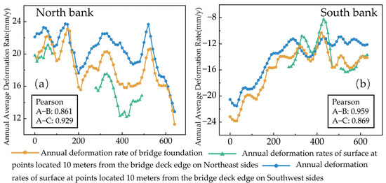
Figure 9.
Comparison of annual average deformation rates of bridge foundations on the north bank (a) and south bank (b) with surrounding ground deformation rates.
5. Discussion
5.1. Relationship Between Uneven Bridge Foundation Settlement and Soil Layer Heterogeneity
The weathered layer at the bridge foundation is mainly composed of Quaternary loess intercalated with gravel. The gravel consists of purplish andesitic rock that has weathered into breccia. The complexity and diversity of the geological environment are among the main causes of uneven settlement [64]. Since the foundation is composed of soil layers with varying thicknesses and properties, it exhibits significant uneven structural settlement [65]. Differences in compressibility, compactness, and bearing capacity of soil layers are direct causes of uneven settlement. Variations in grain composition, porosity, and permeability among different soil layers can affect soil deformation behavior under external loads [66].
According to geological drilling data around the bridge foundation, provided by the Physical Geology Data Center of Natural Resources under the China Geological Survey, the thickness of the same stratigraphic layers varies significantly among different survey points. With increasing distance from the riverbed, the thickness of the weathered layer gradually decreases, while that of the shale and sandstone layers increases correspondingly. Generally, the weathered layer has lower bearing capacity and higher compressibility [67]. Therefore, in areas farther from the riverbed, where the weathered layer is thinner, the underlying soil layers are relatively more solid. Shale and sandstone layers are usually harder and more stable than the weathered layer; thicker shale and sandstone layers provide better foundation support, helping to reduce uneven settlement. However, the mechanical properties of shale and sandstone may still vary due to differences in the degree of weathering or geological structure; such intrinsic differences may also lead to the uneven settlement of the bridge foundation.
5.2. Relationship Between Uneven Bridge Foundation Settlement and STI
A high sediment transport capacity, as indicated by STI, is often accompanied by rapid changes in the riverbed, including frequent erosion and deposition [68,69]. If a bridge foundation is situated in such a dynamic environment, the surrounding foundation materials may be weakened by erosion, leading to uneven settlement. In regions with high STI, water flow may carry away fine-grained soils around the foundation, reducing local support strength and increasing settlement. Conversely, redeposition of sediments may cause uneven load increases around the foundation, leading to additional settlement [70]. Over time, changes in river paths, depths, and widths under high STI conditions can have significant impacts on the bridge foundation. Continuous changes in river courses may also induce heterogeneity in the supporting soil beneath piers or abutments [71].
Figure 10a,c display the observation point data for the north and south banks, respectively. The content represented by the horizontal axis in Figure 10 is consistent with that in Figure 9. Analysis of the north bank reveals that the STI values in this region exhibit significant fluctuations, with two main peak areas. The annual average deformation rate is relatively stable but shows a slight downward trend in regions with higher STI values. In the region with the highest STI values (approximately points 15–20), there is a noticeable decrease in the annual average deformation rate. Overall, there is a negative correlation between STI values and the annual average deformation rate, but this relationship is not entirely linear. In the south bank region, the STI values vary more drastically, with multiple distinct peaks and troughs. The changes in the annual average deformation rate are also more significant, showing an overall upward trend. However, in areas with higher STI values (such as points 100–110 and 125–128), the annual average deformation rate shows a noticeable decrease. Compared to the north bank, the negative correlation on the south bank is more evident, especially in regions where STI values fluctuate greatly. In summary, there is a negative correlation between STI values and the annual average deformation rate; that is, the higher the STI value, the lower the annual average deformation rate. This relationship is more pronounced on the south bank, possibly due to geological conditions or environmental factors in that region. The polar chart in the figure illustrates the relationship between the annual average deformation rate and the STI, providing a more intuitive visualization of their correlations. We employed a nonlinear regression model to analyze the relationship between STI and AADR, calculating the MSE and the between them. An MSE value closer to 0 indicates better model selection and fit, resulting in more successful data predictions. is a statistical indicator used to assess the goodness of fit of a linear regression model, representing the proportion of variance in the dependent variable explained by the predictive values, ranging from 0 to 1 [72]. When the value approaches 1, the model demonstrates a good fit; conversely, a value close to 0 indicates minimal explanatory power. The calculations revealed that the MSE and values for the north bank were 2.64 and 0.43, respectively, while for the south bank, they were 2.54 and 0.54, indicating that both data prediction and fitting performance were satisfactory.
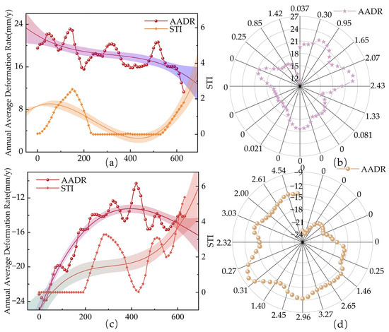
Figure 10.
Correlation between foundation settlement rates and STI values: Annual settlement rates versus STI for the north (a) and south banks (c) (64 points each), with regression fits and 95% confidence intervals. Spatial evolution of settlement rates and STI values across north bank (b) and south banks (d) at selected monitoring points.
5.3. Relationship Between Uneven Bridge Foundation Settlement and TWI
There is a correlation between uneven bridge foundation settlement and TWI, which can be analyzed by examining the impact of TWI on surface hydrological processes. TWI is an index that describes the influence of topography on moisture accumulation and flow, commonly used to predict soil moisture distribution and potential water flow paths. Studies have shown that areas with higher TWI values typically have wetter soils [73]. This may lead to reduced soil bearing capacity, increasing the risk of foundation settlement. Moist soils, especially clayey soils, are more prone to compressive deformation, which can cause the uneven settlement of bridge foundations. Additionally, areas with higher TWI values are often channels where water converges, making them more susceptible to erosion [74]. Erosion can alter the structure and composition of foundation soils, leading to uneven settlement. Continuous erosion may further weaken the stability of the bridge foundation.
Figure 11a,c display data from observation points on the north and south banks, respectively. The content represented by the horizontal axis in Figure 11 is consistent with that in Figure 9. Analysis of the north bank shows that TWI values exhibit a fluctuating upward trend, increasing from approximately 6.71 to 7.12. The annual average deformation rate shows a decreasing trend, declining from about 22 mm/year to 11 mm/year. There is a positive correlation between TWI values and deformation rates, but the relationship is not entirely linear. In areas where TWI values decrease sharply (e.g., points 16–24), the deformation rate decreases significantly. In segments where TWI rises, the deformation rate also increases. However, in the region of points 55–64, TWI values increase while the deformation rate decreases, possibly influenced by other factors.
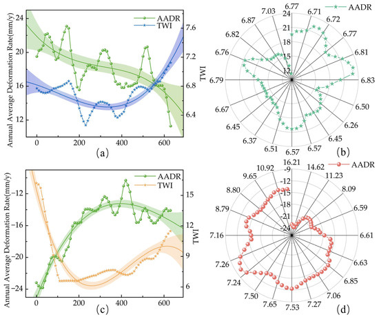
Figure 11.
Correlation analysis of foundation settlement and TWI: Annual settlement rates versus TWI for the north (a) and south banks (c) (n = 64 each), with regression fits and confidence bands. Spatial evolution of settlement rates and corresponding TWI distributions across the north (a) and south banks (c).
In the south bank area, TWI values change more dramatically, decreasing from approximately 16.21 to 6.59 and then rising to 11.49. The annual average deformation rate shows an upward trend, increasing from approximately –23 mm/year to –14 mm/year. The relationship between TWI values and deformation rates is more complex on the south bank, with different segments showing varying correlations. In the middle segment with lower TWI values (approximately points 80–110), the deformation rate remains relatively stable. Overall, there are significant differences in the range and variation patterns of TWI values between the north and south banks, reflecting different topographical and hydrological conditions. The relationship between TWI values and deformation rates also differs between the two banks, suggesting that local geological conditions and other environmental factors may have significant impacts. Generally, areas with higher TWI values often correspond to higher deformation rates. The polar chart in the figure illustrates the relationship between the annual average deformation rate and the TWI, providing a more intuitive visualization of their correlations. We employed a nonlinear regression model to analyze the relationship between TWI and AADR. The calculated MSE and values for the north bank were 2.71 and 0.50, respectively, while for the south bank, they were 2.63 and 0.33. These results indicate that both data prediction and the goodness of fit are satisfactory.
5.4. Relationship Between Uneven Bridge Foundation Settlement and Relative Humidity
Increased precipitation leads to higher soil moisture, thereby reducing soil bearing capacity. Continuous rainfall may cause the groundwater level to rise, increasing pore water pressure and reducing the soil’s effective stress [75]. These changes can decrease soil bearing capacity, thereby causing uneven foundation settlement. Additionally, some geological materials may soften under long-term water erosion; precipitation can accelerate this process, destabilizing the soil structure around the foundation and causing uneven settlement issues [76].
Relative humidity is a comprehensive indicator related not only to local precipitation but also influenced by other meteorological factors like temperature and wind speed. Therefore, relative humidity can effectively reflect a locality’s overall moisture conditions. Compared to precipitation observations, measuring and acquiring relative humidity data are usually more convenient and continuous since precipitation observations may be intermittent. Additionally, trends in relative humidity changes can approximately reflect precipitation changes. This enables relative humidity to substitute for precipitation to some extent in data analysis and modeling.
Figure 12a,b, respectively, display data from observation points on the north and south banks. It can be seen that there is a negative correlation between relative humidity and settlement values. Specifically, higher relative humidity usually corresponds to lower settlement values; when relative humidity decreases, settlement values increase. The figures also show that relative humidity exhibits obvious seasonal variations, higher in summer (July–September) and lower in winter (December–February). Settlement values also exhibit corresponding seasonal characteristics but lag behind humidity changes. Furthermore, we calculated the correlations of observation points P1 to P12. As shown in Table 2, the correlation coefficients between the cumulative deformations at each point and the bridge relative humidity reach 0.51 or higher.
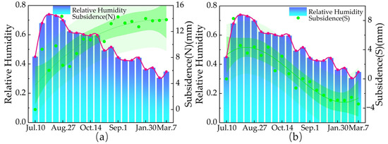
Figure 12.
Correlation between foundation settlement and relative humidity: time-series analysis of the north (a) and south bank (b) monitoring points with 95% confidence and prediction intervals (dark and light shading, respectively).
Table 2.
Correlation coefficient between relative humidity and settlement value.
We conducted a linear regression analysis of relative humidity and settlement values, calculating the Beta, , and p-values, and performed a t-test. The Beta coefficient helps us understand the relationship between the independent and dependent variables [77]. A larger effect of the independent variable on the dependent variable will yield a higher Beta value; conversely, a smaller effect will result in a lower Beta value. The p-value refers to the probability of obtaining a result at least as extreme as the observed sample results, assuming the null hypothesis is true [78]. A small p-value indicates a low probability of the null hypothesis being true; if a low-probability event occurs, we have grounds to reject the null hypothesis. The smaller the p-value, the stronger the justification for rejection. As the p-value decreases (p < 0.05 or p < 0.01), we gather increasingly strong evidence, and the results of the tests become more significant. The calculations yielded a t-value of −7.26 for the north bank, with a Beta of −0.87, of 0.76, and a p-value of 0.00 (less than 0.01), indicating a significant negative impact of relative humidity on settlement values. For the south bank, the t-value was 8.73, with a Beta of 0.90, of 0.82, and a p-value of 0.00 (less than 0.01), indicating a significant positive impact of relative humidity on settlement values. To demonstrate the potential linear relationships mentioned above, we calculated the Pearson correlation coefficients for the points P1 to P12, with the results presented in Table 2. These results align with the conclusions drawn above, indicating a significant negative correlation between relative humidity and settlement values on the north bank, while a significant positive correlation exists on the south bank.
5.5. Relationship Between Uneven Bridge Foundation Settlement and Temperature
Changes in temperature can cause the expansion and contraction of bridge materials and foundation soils. Especially in permafrost regions, high temperatures can cause soil expansion, while low temperatures lead to contraction [79]. Such changes can result in uneven settlement. Cold regions are often affected by soil freeze–thaw cycles. These cycles cause changes in soil volume. For example, water in the soil expands in volume when it freezes and contracts upon thawing, which may lead to increased settlement. On the other hand, seasonal temperature variations also affect evaporation rates, leading to changes in groundwater levels [80]. Rising groundwater levels alter the effective stress of foundation soils. Together with soil expansion caused by temperature, this influences the settlement of bridge foundations.
Figure 13a,b illustrate the data from observation points on the north and south banks, respectively. We observe a clear negative correlation between dry-bulb temperature and settlement values. Specifically, when the temperature is higher, settlement values are lower; when the temperature decreases, settlement values increase. The dry-bulb temperature shows a distinct seasonal variation. It gradually decreases from the high temperatures of summer (July) to the low temperatures of winter (December–February), and then starts to rise again. The changes in settlement values are opposite, being lower in summer and higher in winter. Notably, in both figures, changes in settlement values lag behind temperature changes to some extent. After the temperature begins to decrease, the settlement values do not increase immediately. Instead, they rise significantly after the temperature has continued to decline for some time. Furthermore, we calculated the correlations for observation points P1 to P12. As shown in Table 3, the correlation coefficients between the cumulative deformations at each point and bridge temperature reach 0.69 or higher.
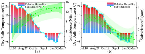
Figure 13.
Settlement–temperature correlation analysis: Time-series settlement response to dry bulb temperature at the north (a) and south bank (b) monitoring points, showing 95% confidence (dark shade) and prediction intervals (light shade).
Table 3.
Correlation coefficient between dry bulb temperature and settlement value.
We employed the same method as that used in the previous study regarding the impact of relative humidity on settlement values. The calculations revealed a t-value of −6.57 for the north bank, with a Beta of −0.84, of 0.71, and a p-value of 0.00 (less than 0.01), indicating a significant negative impact of dry bulb temperature on settlement values. For the south bank, the t-value was 10.06, with a Beta of 0.93, of 0.86, and a p-value of 0.00 (less than 0.01), indicating a significant positive impact of dry bulb temperature on settlement values. To illustrate the potential linear relationships on both banks, we calculated the Pearson correlation coefficients for the previously mentioned points P1 to P12, with the results presented in Table 2. The results are consistent with the previous conclusions, indicating a significant negative correlation between dry bulb temperature and settlement values on the north bank, while a significant positive correlation exists on the south bank.
5.6. Interactions Among Different Factors Affecting Settlement
To determine the interaction effect between STI and TWI, we employed a nonlinear regression model to analyze their MSE, , and p-values. On the north bank, the MSE, , and p-values were 0.04, 0.14, and 0.01, respectively; on the south bank, they were 1.48, 0.13, and 0.0019, respectively. This indicates that the correlation between the two is not high, and their joint effect on AADR is also not significant.
To assess the interaction effect between dry bulb temperature and relative humidity, we introduced the TLCC index. The TLCC is measured by incrementally shifting a time series vector and repeatedly calculating the correlation between the two signals. In this analysis, we selected hourly data for dry bulb temperature and relative humidity during the study period.
Figure 14 indicates a high correlation between dry bulb temperature and relative humidity at the points marked by the pink line.
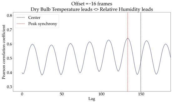
Figure 14.
Correlation between dry bulb temperature and relative humidity.
To assess finer-grained dynamic changes, this study calculated WTLCC. This process involves repeatedly calculating the time-lagged cross-correlation across multiple time windows [81]. Each window can then be analyzed individually, or the sums across windows can be taken to provide a score for comparing the differences in interaction between leaders and followers. As shown in Figure 15a, the time series is divided into 20 equal-length segments, and the cross-correlation for each time window is calculated. In the first window (first row), the red peak indicates that dry bulb temperature is leading the interaction, while the blue peak suggests that relative humidity is beginning to lead the interaction more [82]. As illustrated in Figure 15b, the time series is divided into more segments, and the cross-correlation for each time window is calculated. This provides us with a finer-grained perspective to observe the interactions between the two variables. The alternating blue and red colors in the figure indicate an alternating leading relationship between the two variables.
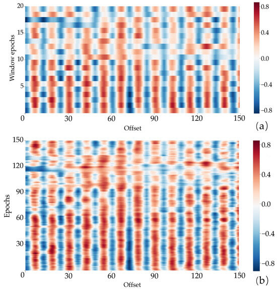
Figure 15.
(a) Windowed time-lagged cross correlation. (b) Moving windowed time-lagged cross correlation. Window epochs mean different time windows.
We calculated the VIF for dry bulb temperature and relative humidity, as well as conducted the Durbin–Watson (D-W) test. The VIF is a measure of the severity of multicollinearity in multiple linear regression models. Multicollinearity refers to the linear relationship that exists between independent variables, meaning that one independent variable can be expressed as a linear combination of one or more independent variables. If multicollinearity is present, the matrix will be non-invertible when calculating the partial regression coefficients of the independent variables. The D-W value plays an important role in statistics, primarily in the field of regression analysis, specifically referring to the difference between the residuals and the predicted values [83]. This difference is a key indicator of the model’s predictive accuracy. The D-W value helps us assess whether the regression model effectively captures the trends in the data during prediction. A D-W value close to 2 indicates that the model predictions are relatively accurate and there is no significant autocorrelation among the residuals. The calculated VIF values for the north bank and south bank were 3.032 and 3.523, respectively, indicating that there is no multicollinearity between them. Additionally, the D-W values for both banks were near 2, indicating that there is no autocorrelation present.
6. Conclusions
This study systematically analyzed uneven settlement in long-span bridge foundations using SBAS-InSAR technology, combined with geological borehole data, DEM data, temperature, and humidity data. The main conclusions are as follows:
- (1)
- Analysis of Uneven Foundation Settlement Using SBAS-InSAR Technology: The uneven foundation settlement of Huailai Bridge was analyzed using SBAS-InSAR technology. The results indicate that the north bank approach bridge foundation and the north side foundation of the main bridge generally exhibited an uplift trend. In contrast, the south side foundation of the main bridge and the south bank approach bridge foundation tended to subside, demonstrating a complex deformation pattern.
- (2)
- Influence of Various Factors on Foundation Settlement: By analyzing factors such as geological conditions, Sediment Transport Index (STI), Topographic Wetness Index (TWI), relative humidity, and temperature, we found that these factors may influence bridge foundation settlement. Stratigraphic heterogeneity, dynamic hydrological environments, and seasonal climate changes are potential causes of uneven settlement. Among the factors considered, relative humidity and temperature have a significant impact on foundation settlement.
- (3)
- Effectiveness of SBAS-InSAR Technology in Monitoring Dynamic Deformation: SBAS-InSAR technology can effectively monitor the dynamic deformation of bridges, providing reliable data support for bridge safety assessments. The results of this study indicate that SBAS-InSAR is an effective tool for surface deformation monitoring, providing a scientific basis for analysis and early warning of foundation settlement in long-span bridges.
The methods and findings presented in this study offer new perspectives for analyzing the uneven settlement of long-span bridge foundations and provide important references for bridge safety assessments and preventive maintenance. In the future, the monitoring time span can be extended to explore the dynamic characteristics of bridge foundation settlement more deeply. Moreover, future research can investigate different influencing factors, such as stratigraphic structure, hydrological environment, and climate change, to quantitatively analyze the specific mechanisms affecting the rate and direction of bridge foundation settlement. And this research can explore the effects of humidity and temperature under different environmental conditions to gain a more comprehensive understanding of their impacts under varying geographical conditions and climate contexts.
Supplementary Materials
The following supporting information can be downloaded at www.mdpi.com/article/10.3390/rs17020248/s1: Table S1: Technical Specifications of Sentinel-1A SAR Imagery; Figure S1: Acquisition areas for Sentinel-1A SAR imagery.
Author Contributions
All authors contributed to the manuscript and discussed the results. S.N. and K.Z., conceptualization; H.Z., data curation; W.X., software; S.N., S.H. and R.A., supervision; K.Z., H.Z. and D.J., writing—review and editing; B.R.T., software, writing—review and editing. All authors have read and agreed to the published version of the manuscript.
Funding
This work was supported by the National Training Program of Innovation and Entrepreneurship for Undergraduates (grant number: S202410359410), the National Natural Science Foundation of China (42271084), and the Natural Science Foundation of Anhui Province (2208085US15).
Data Availability Statement
The original contributions presented in the study are included in the article, further inquiries can be directed to the corresponding author.
Acknowledgments
We sincerely thank the European Space Agency for providing the free Sentinel-1A data and POD data. Additionally, we are grateful to NASA for supplying the SRTM3 DEM data. The authors would also like to express their heartfelt appreciation to the anonymous reviewers for their insightful comments and valuable suggestions.
Conflicts of Interest
The authors declare no conflicts of interest.
References
- Zhang, Z.; Leong, E.C.; Gong, W.; Dai, G.; Li, J. Foundation design of single-span arch bridges in China. Case Stud. Constr. Mater. 2023, 19, e02239. [Google Scholar] [CrossRef]
- Nolan, S.; Cadenazzi, T.; Rossini, M.; Nanni, A.; Knight, C.; Lasa, I. The 200-Year Bridge Substructure: Resilience and Sustainability; IABSE Congress: New York, NY, USA, 2019. [Google Scholar] [CrossRef]
- Ostenfeld, K.H. Evolution of Bridge Foundations for Constructability, Economy, Substainability and Safety; IABSE: Lyngby, Demark, 1999; pp. 7–12. [Google Scholar] [CrossRef]
- Hu, X.; Assaad, R.H.; Hussein, M. Discovering key factors and causalities impacting bridge pile resistance using Ensemble Bayesian networks: A bridge infrastructure asset management system. Expert Syst. Appl. 2024, 238, 121677. [Google Scholar] [CrossRef]
- Zhang, D.; Xiong, W.; Ma, X.; Cai, C.S. Fragility Evaluation of Bridge Pile Foundation Considering Scour Development under Floods. J. Bridge Eng. 2024, 29, 04024052. [Google Scholar] [CrossRef]
- Reumers, P.; Lombaert, G.; Degrande, G. The effect of foundation–soil–foundation interaction on the response of continuous, multi-span railway bridges. Eng. Struct. 2024, 299, 117096. [Google Scholar] [CrossRef]
- Li, R.; He, Q.; Zhu, S.; Yan, J.; Zhai, W. A new methodology for pre-camber design of a long-span bridge considering dynamic train load and complex environmental effects. Eng. Struct. 2024, 302, 117349. [Google Scholar] [CrossRef]
- Wang, N.; Elgamal, A.; Lu, J. Seismic response of the Eureka Channel bridge-foundation system. Soil Dyn. Earthq. Eng. 2022, 152, 107015. [Google Scholar] [CrossRef]
- He, Q.; Wang, D.; Peng, N. Numerical analysis of influencing factors of uneven settlement in abutment foundation. Adv. Mat. Res. 2012, 422, 864–868. [Google Scholar] [CrossRef]
- Liu, F.; Zheng, G.; Cui, G. Settlement deformation characteristics and control of soft soil through groundwater discharge zone. Desalin. Water Treat. 2021, 241, 282–287. [Google Scholar] [CrossRef]
- Liu, W.; Yang, X.; Zhang, S.; Kong, X.; Chen, W. Analysis of Deformation Characteristics of Long-Short Pile Composite Foundation in Salt Lake Area, Iran. Adv. Civ. Eng. 2019, 2019, 5976540. [Google Scholar] [CrossRef]
- Du, Y.; He, X.; Wu, C.; Wu, W. Long-term monitoring and analysis of the longitudinal differential settlement of an expressway bridge–subgrade transition section in a loess area. Sci. Rep. 2022, 12, 19327. [Google Scholar] [CrossRef] [PubMed]
- Feng, Y.; Hou, Y.; Jiang, L.; Zhou, W.; Li, H.; Yu, J. Failure mode of interlayer connection of longitudinally-connected ballastless track-bridge system under uneven pier settlement. Constr. Build. Mater. 2022, 351, 128805. [Google Scholar] [CrossRef]
- Sun, H.; Chen, A.; Shi, L.; Cai, Y. Iterative method for predicting uneven bridge approach settlement (BAS) caused by vehicle loads. Math. Probl. Eng. 2020, 2020, 8476746. [Google Scholar] [CrossRef]
- Li, F.; Gong, H.; Chen, B.; Gao, M.; Zhou, C.; Guo, L. Understanding the influence of building loads on surface settlement: A case study in the central business district of Beijing combining multi-source data. Remote Sens. 2021, 13, 3063. [Google Scholar] [CrossRef]
- Wang, Y.; Zhou, H.; Wang, L. Settlement mode analysis for an immersed tube tunnel considering a nonuniform foundation under tidal load. China Ocean Eng. 2022, 36, 427–438. [Google Scholar] [CrossRef]
- Yang, W.; Ma, L. Research on Common Diseases and Construction Treatment Technologies in Road and Bridge Engineering. AJST 2024, 10, 42–45. [Google Scholar] [CrossRef]
- Fu, X.; Li, J.; Liu, J.; Hu, Z.; Tang, C. Influence of Complex Hydraulic Environments on the Mechanical Properties of Pile-Soil Composite Foundation in the Coastal Soft Soil Area of Zhuhai. Buildings 2023, 13, 563. [Google Scholar] [CrossRef]
- Wang, L.; Sun, G.; Xu, J.; Wu, X.; Hou, X.; Han, Z. Study on Arching Mechanism of Bridge Pile Foundation: Taking the Shiyangtai No. 1 Bridge as an Example. Buildings 2024, 14, 243. [Google Scholar] [CrossRef]
- Rakoczy, A.M.; Ribeiro, D.; Hoskere, V.; Narazaki, Y.; Olaszek, P.; Karwowski, W. Technologies and Platforms for Remote and Autonomous Bridge Inspection–Review. Struct. Eng. Int. 2024, 1–23. [Google Scholar] [CrossRef]
- Li, J.; Ma, L. Research on Quality Inspection and Reinforcement Technology of Road Bridge. AJST 2024, 10, 51–54. [Google Scholar] [CrossRef]
- Ozden, A.; Faghri, A.; Li, M.; Tabrizi, K. Evaluation of Synthetic Aperture Radar satellite remote sensing for pavement and infrastructure monitoring. Procedia Eng. 2016, 145, 752–759. [Google Scholar] [CrossRef]
- Lorenz, R.; Petryna, Y.; Lubitz, C.; Lang, O.; Wegener, V. Thermal deformation monitoring of a highway bridge: Combined analysis of geodetic and satellite-based InSAR measurements with structural simulations. J. Civ. Struct. Health Monit. 2024, 14, 1237–1255. [Google Scholar] [CrossRef]
- Ferretti, A.; Prati, C.; Rocca, F. Permanent scatterers in SAR interferometry. IEEE Trans. Geosci Remote Sens. 2001, 39, 8–20. [Google Scholar] [CrossRef]
- Hanssen, R.F. Satellite radar interferometry for deformation monitoring: A priori assessment of feasibility and accuracy. Int. J. Appl. Earth OBS 2005, 6, 253–260. [Google Scholar] [CrossRef]
- Martino, G.D.; Esposito, M.; Festa, B.; Iodice, A.; Mancini, L.; Poreh, D. Railway Bridge Monitoring with Sar: A Case Study. In Proceedings of the 2018 IEEE International Geoscience and Remote Sensing Symposium, Valencia, Spain, 22–27 July 2018; IEEE: Geneva, Switzerland, 2018; pp. 2952–2955. [Google Scholar] [CrossRef]
- Cusson, D.; Stewart, H. Satellite Synthetic Aperture Radar, Multispectral, and Infrared Imagery for Assessing Bridge Deformation and Structural Health—A Case Study at the Samuel de Champlain Bridge. Remote Sens. 2024, 16, 614. [Google Scholar] [CrossRef]
- Malinowska, D.; Milillo, P.; Briggs, K.; Reale, C.; Giardina, G. Coherence-Based Prediction of Multi-Temporal InSAR Measurement Availability for Infrastructure Monitoring. IEEE J. Sel. Top. Appl. Earth OBS Remote Sens. 2024, 17, 16392. [Google Scholar] [CrossRef]
- Lazecky, M.; Perissin, D.; Bakon, M.; De Sousa, J.M.; Hlavacova, I.; Real, N. Potential of satellite InSAR techniques for monitoring of bridge deformations. In Proceedings of the 2015 Joint Urban Remote Sensing Event (JURSE), Lausanne, Switzerland, 30 March–1 April 2015. [Google Scholar] [CrossRef]
- Selvakumaran, S.; Rossi, C.; Marinoni, A.; Webb, G.; Bennetts, J.; Barton, E. Combined InSAR and terrestrial structural monitoring of bridges. IEEE Trans. Geosci. Remote Sens. 2020, 58, 7141–7153. [Google Scholar] [CrossRef]
- Nettis, A.; Massimi, V.; Nutricato, R.; Nitti, D.O.; Samarelli, S.; Uva, G. Satellite-based interferometry for monitoring structural deformations of bridge portfolios. Automat. Constr. 2023, 147, 104707. [Google Scholar] [CrossRef]
- Matteo, D.S.; Roberto, T.; Javier, P.C.; Gerardo, H.G.; Juan Carlos, G.L.D.; Oscar, M. A multi-sensor approach for monitoring a road bridge in the Valencia harbor (SE Spain) by SAR Interferometry (InSAR). Rend. Online Soc. Geol. 2016, 41, 235–238. [Google Scholar] [CrossRef]
- Du, Y.; Feng, D.; Wu, G. InSAR-based rapid damage assessment of urban building portfolios following the 2023 Turkey earthquake. Int. J. Disaster Risk Reduct. 2024, 103, 104317. [Google Scholar] [CrossRef]
- Macchiarulo, V.; Milillo, P.; Blenkinsopp, C.; Reale, C.; Giardina, G. Multi-temporal InSAR for transport infrastructure monitoring: Recent trends and challenges. Proc. Inst. Civ. Eng.-BR 2021, 176, 92–117. [Google Scholar] [CrossRef]
- Zhao, X.; Zhu, S.; Sun, W.; Huang, Z. Application of PS-InSAR technology in bridge settlement deformation monitoring. CN11-4527/TU 2023, 41, 54–60. [Google Scholar] [CrossRef]
- Wang, C.; Zhou, L.; Ma, J.; Shi, A.; Li, X.; Liu, L.; Zhang, Z.; Zhang, D. GB-RAR deformation information estimation of high-speed railway bridge in consideration of the effects of colored noise. Appl. Sci. 2022, 12, 10504. [Google Scholar] [CrossRef]
- Selvakumaran, S.; Plank, S.; Geiß, C.; Rossi, C.; Middleton, C. Remote monitoring to predict bridge scour failure using Interferometric Synthetic Aperture Radar (InSAR) stacking techniques. Int. J. Appl. Earth OBS 2018, 73, 463–470. [Google Scholar] [CrossRef]
- Guzman-Acevedo, G.M.; Quintana-Rodriguez, J.A.; Gaxiola-Camacho, J.R.; Vazquez-Becerra, G.E.; Torres-Moreno, V.; Monjardin-Quevedo, J.G. The Structural Reliability of the Usumacinta Bridge Using InSAR Time Series of Semi-Static Displacements. Infrastructures 2023, 8, 173. [Google Scholar] [CrossRef]
- Jiang, H.; Balz, T.; Cigna, F.; Tapete, D.; Li, J.; Han, Y. Multi-sensor InSAR time series fusion for long-term land subsidence monitoring. Geo. Spat. Inf. Sci. 2023, 27, 1424–1440. [Google Scholar] [CrossRef]
- Zhao, C.; Peng, M.; Zhu, J. Application of Persistent Scatterer Interferometric Synthetic Aperture Radar in Bridge Settlement Monitoring. Road Mach. Constr. Mech. 2019, 36, 115–120. [Google Scholar] [CrossRef]
- Lasri, O.; Giordano, P.F.; Limongelli, M.P.; Previtali, M. Remote monitoring of a concrete bridge using PSInSAR. ce/papers 2023, 6, 893–899. [Google Scholar] [CrossRef]
- Ma, P.; Wu, Z.; Zhang, Z.; Au, F.T.K. SAR-Transformer-based decomposition and geophysical interpretation of InSAR time-series deformations for the Hong Kong-Zhuhai-Macao Bridge. Remote Sens. Environ. 2024, 302, 113962. [Google Scholar] [CrossRef]
- Du, Y.; Yan, S.; Zhao, F.; Chen, D.; Zhang, H. DS-InSAR based long-term deformation pattern analysis in the mining region with an improved phase optimization algorithm. Front. Environ. Sci. 2022, 10, 799946. [Google Scholar] [CrossRef]
- Li, S.; Xu, W.; Li, Z. Review of the SBAS InSAR Time-series algorithms, applications, and challenges. Geod. Geodyn. 2022, 13, 114–126. [Google Scholar] [CrossRef]
- Berardino, P.; Fornaro, G.; Lanari, R.; Sansosti, E. A new algorithm for surface deformation monitoring based on small baseline differential SAR interferograms. IEEE Trans. Geosci. Remote Sens. 2002, 40, 2375–2383. [Google Scholar] [CrossRef]
- Wang, R.; Feng, Y.; Tong, X.; Li, P.; Wang, J.; Tang, P.; Tang, X.; Xi, M.; Zhou, Y. Large-Scale Surface Deformation Monitoring Using SBAS-InSAR and Intelligent Prediction in Typical Cities of Yangtze River Delta. Remote Sens. 2023, 15, 4942. [Google Scholar] [CrossRef]
- Han, Z. Research on Surface Deformation Monitoring Using SBAS-InSAR: A Case Study of Zhujiang Bridge in Nansha District, Guangzhou. J. ACM 2023, 13, 1–6. [Google Scholar] [CrossRef]
- Zhou, L.; Li, X.; Pan, Y.; Ma, J.; Wang, W.; Shi, A.; Chen, Y. Deformation monitoring of long-span railway bridges based on SBAS-InSAR technology. Geod. Geodyn. 2024, 15, 122–132. [Google Scholar] [CrossRef]
- The Provincial Highway S228 Langzhen Line Huailai Bridge Officially Opened to Traffic Today! Available online: https://www.thepaper.cn/newsDetail_forward_13344674 (accessed on 6 October 2024).
- Yu, Z.; Zhang, G.; Huang, G.; Cheng, C.; Zhang, Z.; Zhang, C. SSBAS-InSAR: A Spatially Constrained Small Baseline Subset InSAR Technique for Refined Time-Series Deformation Monitoring. Remote Sens. 2024, 16, 3515. [Google Scholar] [CrossRef]
- He, Y.; Wang, W.; Zhang, L.; Chen, Y.; Chen, Y.; Chen, B.; He, X.; Zhao, Z. An identification method of potential landslide zones using InSAR data and landslide susceptibility. Geomat. Nat. Haz. Risk 2023, 14, 2185120. [Google Scholar] [CrossRef]
- Zhang, S.; Wang, J.; Feng, Z.; Wang, T.; Li, J.; Liu, N. Verification of the accuracy of Sentinel-1 for DEM extraction error analysis under complex terrain conditions. Int. J. Appl. Earth OBS Geoinf. 2024, 133, 104157. [Google Scholar] [CrossRef]
- Hu, H.; Fu, H.; Zhu, J.; Liu, J.; Wu, K.; Zeng, D.; Wan, A.; Wang, F. Automatic Correction of Time-Varying Orbit Errors for Single-Baseline Single-Polarization InSAR Data Based on Block Adjustment Model. Remote Sens. 2024, 16, 3578. [Google Scholar] [CrossRef]
- Feng, Y.; Zhou, Y.; Chen, Y.; Li, P.; Xi, M.; Tong, X. Automatic selection of permanent scatterers-based GCPs for refinement and reflattening in InSAR DEM generation. Int. J. Digit. Earth 2022, 15, 954–974. [Google Scholar] [CrossRef]
- Wang, Z.; Liu, F.; Zeng, T.; Wang, C. Interferometric phase error analysis and compensation in GNSS-InSAR: A case study of structural monitoring. Remote Sens. 2021, 13, 3041. [Google Scholar] [CrossRef]
- Gaurav Singh, V.; Singh, S.K. Analysis of geo-morphometric and topo-hydrological indices using COP-DEM: A case study of Betwa River Basin, Central India. Geol. Ecol. Landsc. 2024, 8, 101–128. [Google Scholar] [CrossRef]
- Liu, H.; Li, Y.; Liu, C.; Shen, G.; Xiang, H. Pavement distress initiation prediction by time-lag analysis and logistic regression. Appl. Sci. 2022, 12, 11855. [Google Scholar] [CrossRef]
- Chaikul, S.; Khunatorn, Y.; Phithakkitnukoon, S. A Study of Temporal Correlation Between Space Utilization and Electricity Consumption in Buildings Using Wi-Fi Probe Data. IEEE Access 2024, 12, 105792–105802. [Google Scholar] [CrossRef]
- Zhao, L.; Faust, R.A.; David, R.E.; Norton, J.; Xagoraraki, I. Tracking the Time Lag between SARS-CoV-2 Wastewater Concentrations and Three COVID-19 Clinical Metrics: A 21-Month Case Study in the Tricounty Detroit Area, Michigan. J. Environ. Eng. 2024, 150, 06023004. [Google Scholar] [CrossRef]
- Li, R.; Feng, K.; An, T.; Cheng, P.; Wei, L.; Zhao, Z.; Xu, X.; Zhu, L. Enhanced Insights into Effluent Prediction in Wastewater Treatment Plants: Comprehensive Deep Learning Model Explanation Based on SHAP. ACS EST Water 2024, 4, 1904–1915. [Google Scholar] [CrossRef]
- Zhang, Z.; Chen, G.; Kusky, T.; Yang, J.; Cheng, Q. Lithospheric thickness records tectonic evolution by controlling metamorphic conditions. Sci. Adv. 2023, 9, eadi2134. [Google Scholar] [CrossRef]
- Debnath, J.; Sahariah, D.; Nath, N.; Saikia, A.; Lahon, D.; Islam, M.N.; Hashimoto, S.; Meraj, G.; Kumar, P.; Singh, S.K.; et al. Modelling on assessment of flood risk susceptibility at the Jia Bharali River basin in Eastern Himalayas by integrating multicollinearity tests and geospatial techniques. Model. Earth Syst. Environ. 2024, 10, 2393–2419. [Google Scholar] [CrossRef]
- Zou, L.; Feng, W.; Masci, O.; Nico, G.; Alani, A.M.; Sato, M. Bridge Monitoring Strategies for Sustainable Development with Microwave Radar Interferometry. Sustain. Sci. 2024, 16, 2607. [Google Scholar] [CrossRef]
- Zhang, L.; Wu, X.; Chen, Q.; Skibniewski, M.J.; Hsu, S.C. Towards a safety management approach for adjacent buildings in tunneling environments: Case study in China. Build. Environ. 2014, 75, 222–235. [Google Scholar] [CrossRef]
- Mitchell, J.K.; Soga, K. Fundamentals of Soil Behavior, 3rd ed.; John Wiley & Sons, Ltd.: Hoboken, NJ, USA, 2005; pp. 18–25. Available online: https://istasazeh-co.com/wp-content/uploads/2022/04/Fundamentals-Of-Soil-Behavior-K-Mitchel.pdf (accessed on 11 November 2024).
- Nujid, M.M.; Tholibon, D.A.; Mukhlisin, M. Geotechnical and structural assessment on estimated bearing capacity of strip footing resting on silty sand incorporating moisture content effect. Case Stud. Constr. Mater. 2024, 20, e03106. [Google Scholar] [CrossRef]
- Hosseinpour, I.; Almeida, M.S.S.; Riccio, M.; Baroni, M. Strength and compressibility characteristics of a soft clay subjected to ground treatment. Geotech. Geol. Eng. 2017, 35, 1051–1066. [Google Scholar] [CrossRef]
- Mrad, D.; Boukhari, S.; Dairi, S.; Djebbar, Y. Mapping the Potential for Erosion Gullies Using Frequency Ratio and Fuzzy Analytical Hierarchy Process: Case Study Medjerda Basin, Northeast Algeria. Eurasian Soil Sci. 2024, 57, 1381–1391. [Google Scholar] [CrossRef]
- Yao, C.; Zhang, Q.; Wang, C.; Ren, J.; Li, H.; Wang, H.; Wu, F. Response of sediment transport capacity to soil properties and hydraulic parameters in the typical agricultural regions of the Loess Plateau. Sci. Total Environ. 2023, 879, 163090. [Google Scholar] [CrossRef]
- Hagiwara, T.; Aita, S.; Kazama, S. Impact of Filter Unit Placement on Suspended Sediment Deposition Promotion in Rivers. J. Hydraul. Eng. 2024, 150, 04024043. [Google Scholar] [CrossRef]
- Leopold, L.B.; Wolman, M.G.; Miller, J.P.; Wohl, E.E. Fluvial Processes in Geomorphology, 2nd ed.; Courier Dover Publications: New York, NY, USA, 2020; pp. 284–304. Available online: https://books.google.com.hk/books?hl=en&lr=&id=vnb2DwAAQBAJ&oi=fnd&pg=PA3&dq=fluvial+processes+in+geomorphology+2020&ots=znSNXNoq7g&sig=ZdNWbUiZjlWVul7IjMyUtxOmpjw&redir_esc=y#v=onepage&q=fluvial%20processes%20in%20geomorphology%202020&f=false (accessed on 11 November 2024).
- King, M.; Kim, B.J.; Yune, C.Y. Prediction model of undisturbed ground temperature using artificial neural network (ANN) and multiple regressions approach. Geothermics 2024, 119, 102945. [Google Scholar] [CrossRef]
- Hesterah, H.; Plantak, M.; Gernhardt, D. Correlations Between Topographic Wetness Index and Soil Moisture in The Pannonian Region of Croatia. Geogr. Tech. 2024, 19, 89–102. [Google Scholar] [CrossRef]
- Gidafie, D.; Nedaw, D.; Azagegn, T. Integrated remote sensing and geographic information system overlay analysis for groundwater potential evaluation using AHP and fuzzy AHP: Southern sections of the western Afar rift margin and associated rift floor. Groundw. Sustain. Dev. 2024, 26, 101310. [Google Scholar] [CrossRef]
- Kluger, M.O.; Jorat, M.E.; Moon, V.G.; Kreiter, S.; De Lange, W.P.; Mörz, T.; Robertson, T.; Lowe, D.J. Rainfall threshold for initiating effective stress decrease and failure in weathered tephra slopes. Landslides 2020, 17, 267–281. [Google Scholar] [CrossRef]
- Firoozi, A.A.; Firoozi, A.A. Water Erosion Processes: Mechanisms, Impact, and Management Strategies. Result Eng. 2024, 24, 103237. [Google Scholar] [CrossRef]
- Jabbar, M.; Nasar-u-Minallah, M.; Yusoff, M.M. Measuring and modeling the association between human psychological well-being and urban green spaces of Lahore, Pakistan. J. Environ. Stud. Sci. 2024, 14, 732–743. [Google Scholar] [CrossRef]
- Edmunds, N.S.; Genc, A.G.; McGuffin, L.J. Benchmarking of AlphaFold2 accuracy self-estimates as indicators of empirical model quality and ranking: A comparison with independent model quality assessment programmes. Bioinformatics. 2024, 40, btae491. [Google Scholar] [CrossRef]
- Jabbarzadeh, M.; Sadeghi, H.; Tourchi, S.; Darzi, A.G. Thermo-hydraulic analysis of desiccation cracked soil strata considering ground temperature and moisture dynamics under the influence of soil-atmosphere interactions. Geomech. Energy Environ. 2024, 38, 100558. [Google Scholar] [CrossRef]
- Richardson, C.M.; Davis, K.L.; Ruiz-González, C.; Guimond, J.A.; Michael, H.A.; Paldor, A.; Moosdorf, N.; Paytan, A. The impacts of climate change on coastal groundwater. Nat. Rev. Earth Environ. 2024, 5, 100–119. [Google Scholar] [CrossRef]
- Lei, B.; Song, Y. Volatility forecasting for stock market incorporating media reports, investors’ sentiment, and attention based on MTGNN model. J. Forecast. 2024, 43, 1706–1730. [Google Scholar] [CrossRef]
- Xuan, Y.; Zhu, G.; Luo, X.; Wang, Y.; Wang, L. Experimental Study on the Stability of Mixed-Flow Pump During Segmented Start-Up Process. Arab. J. Sci. Eng. 2024, 1–13. [Google Scholar] [CrossRef]
- Soumena, F.Y.; Umaima, U.; Nurwahida, N.; Syam, D.R.Y. The Influence of SME Funding and Non-Performing Financing on Indonesia’s Economic Growth in The Period 2015–2022. Return Stud. Manag. Econ. Bus. 2024, 3, 166–180. [Google Scholar] [CrossRef]

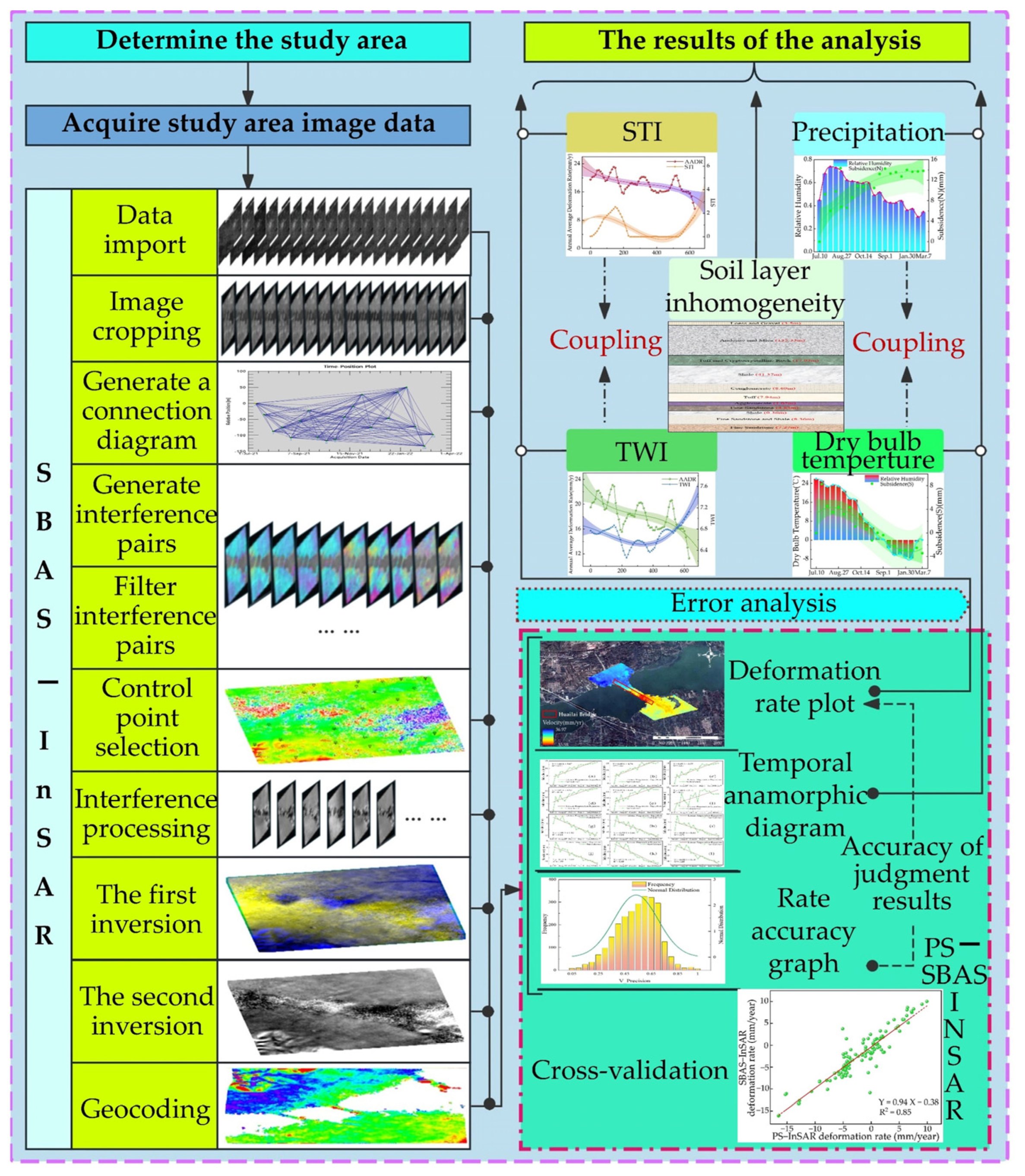
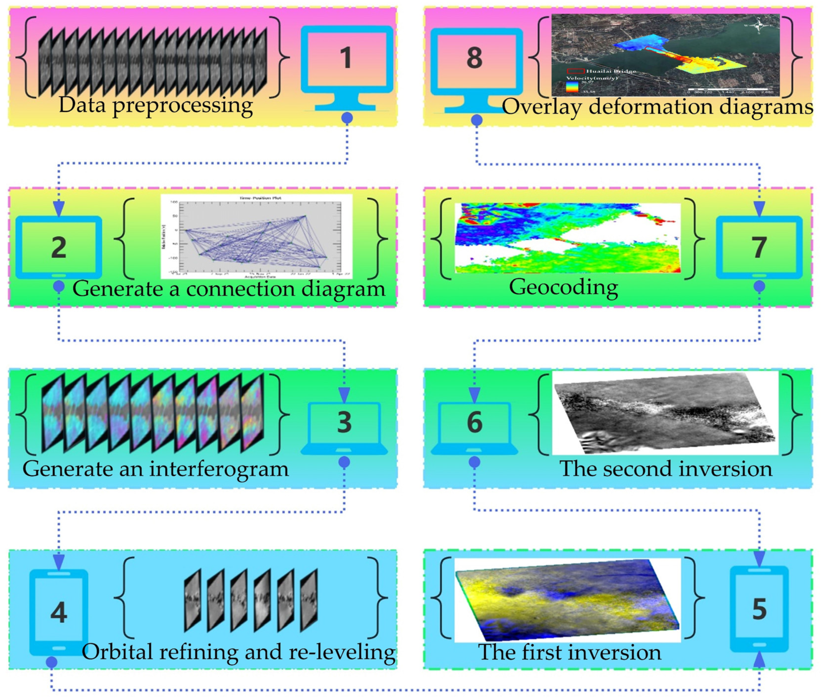


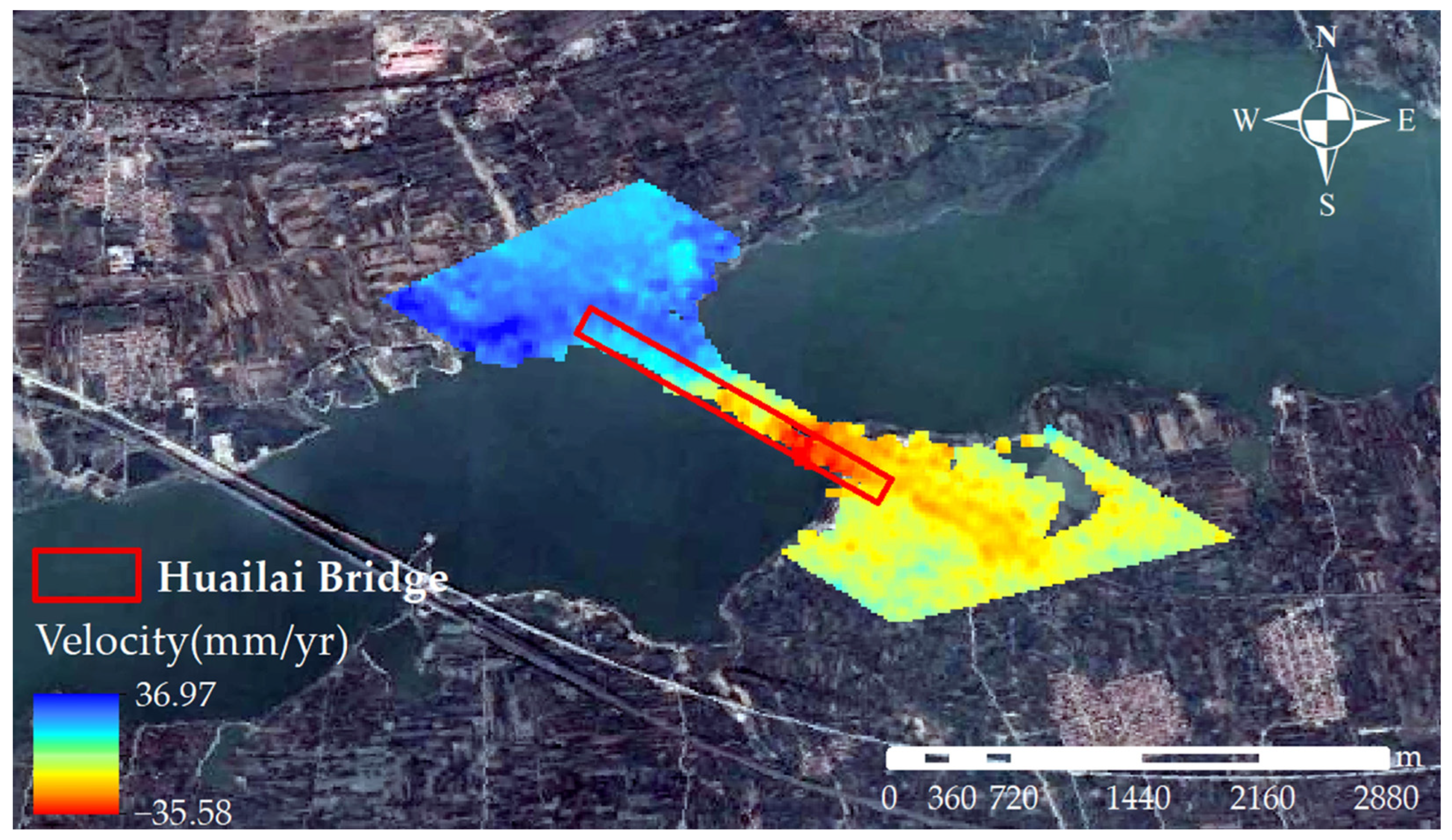
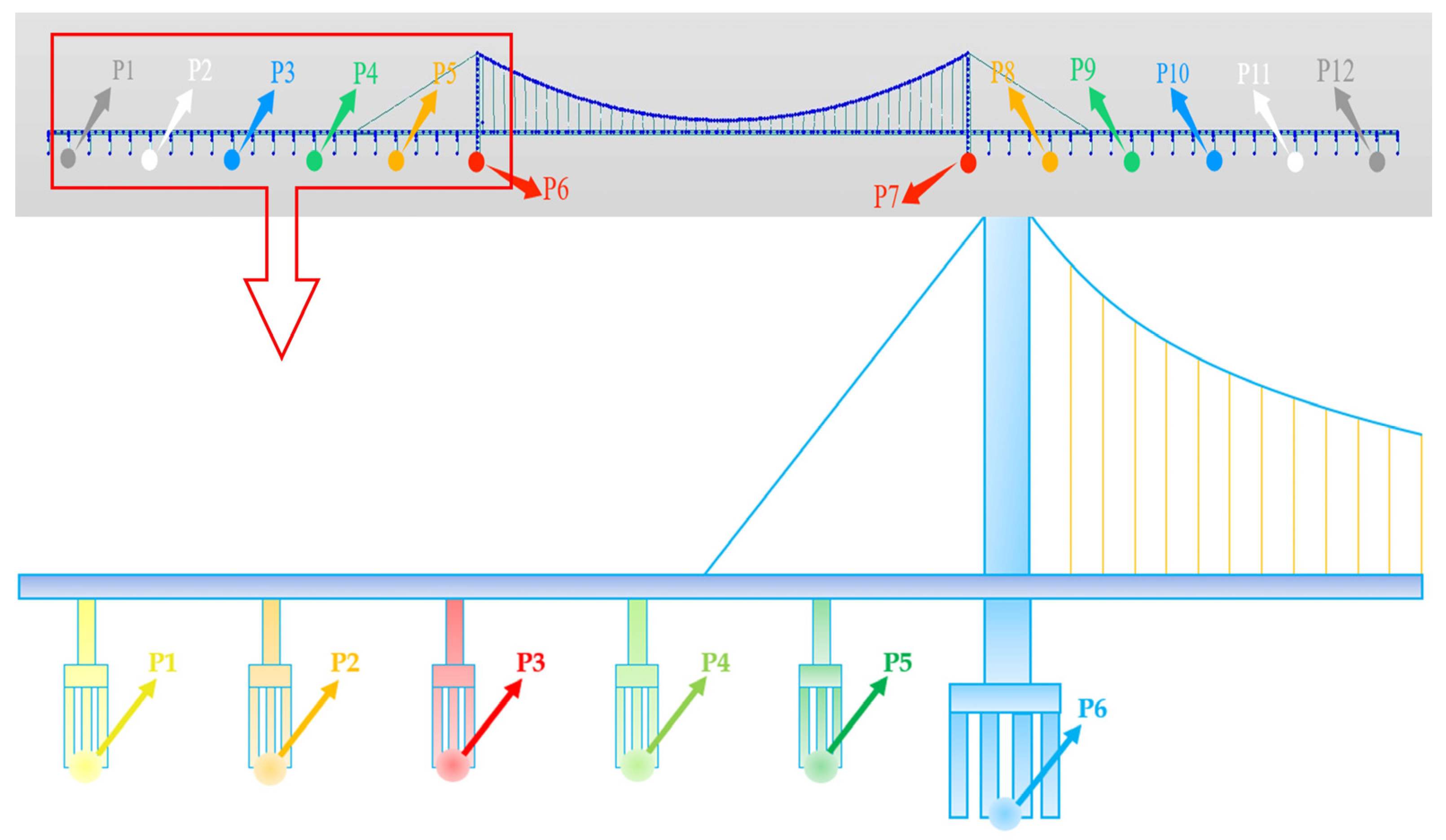
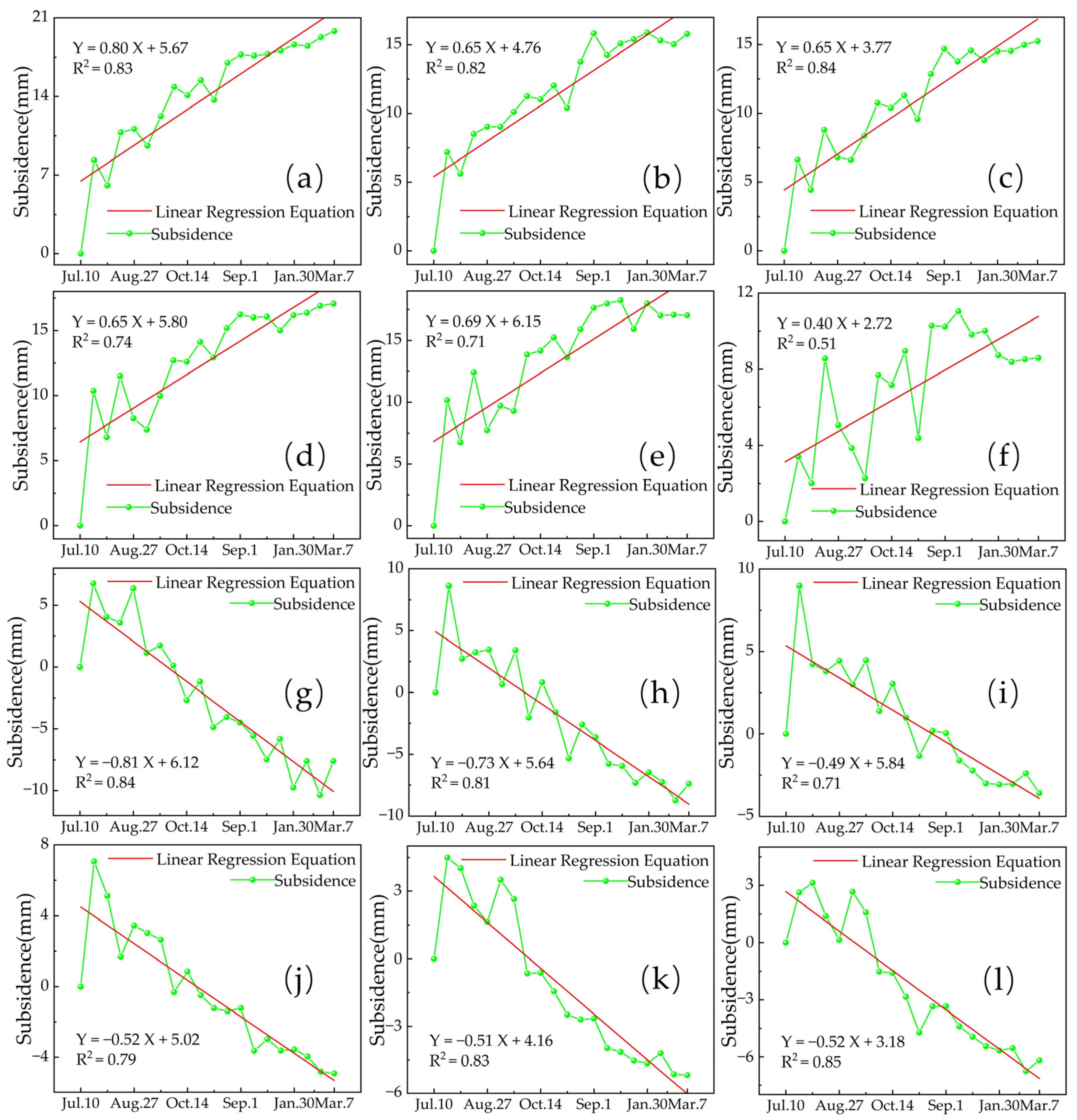
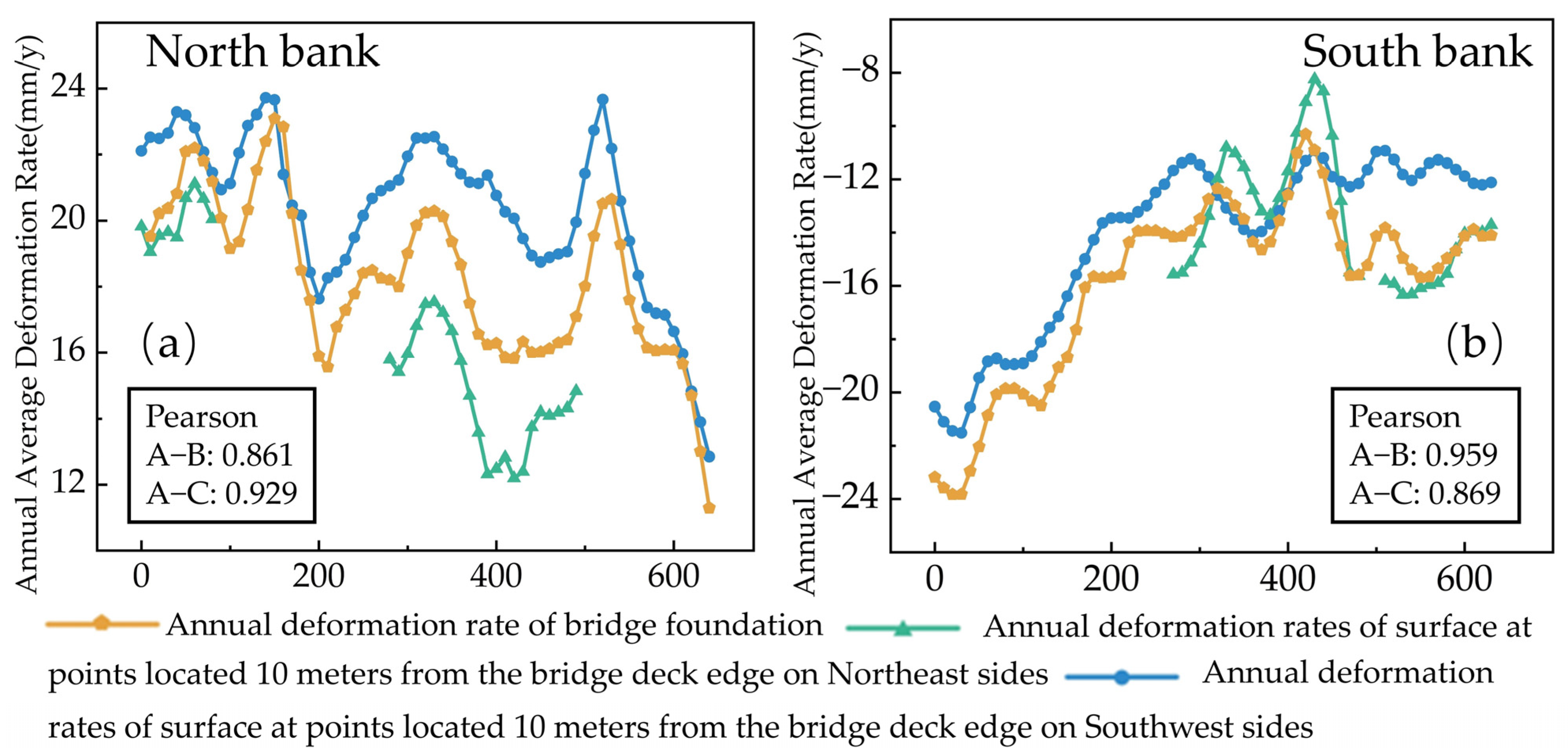
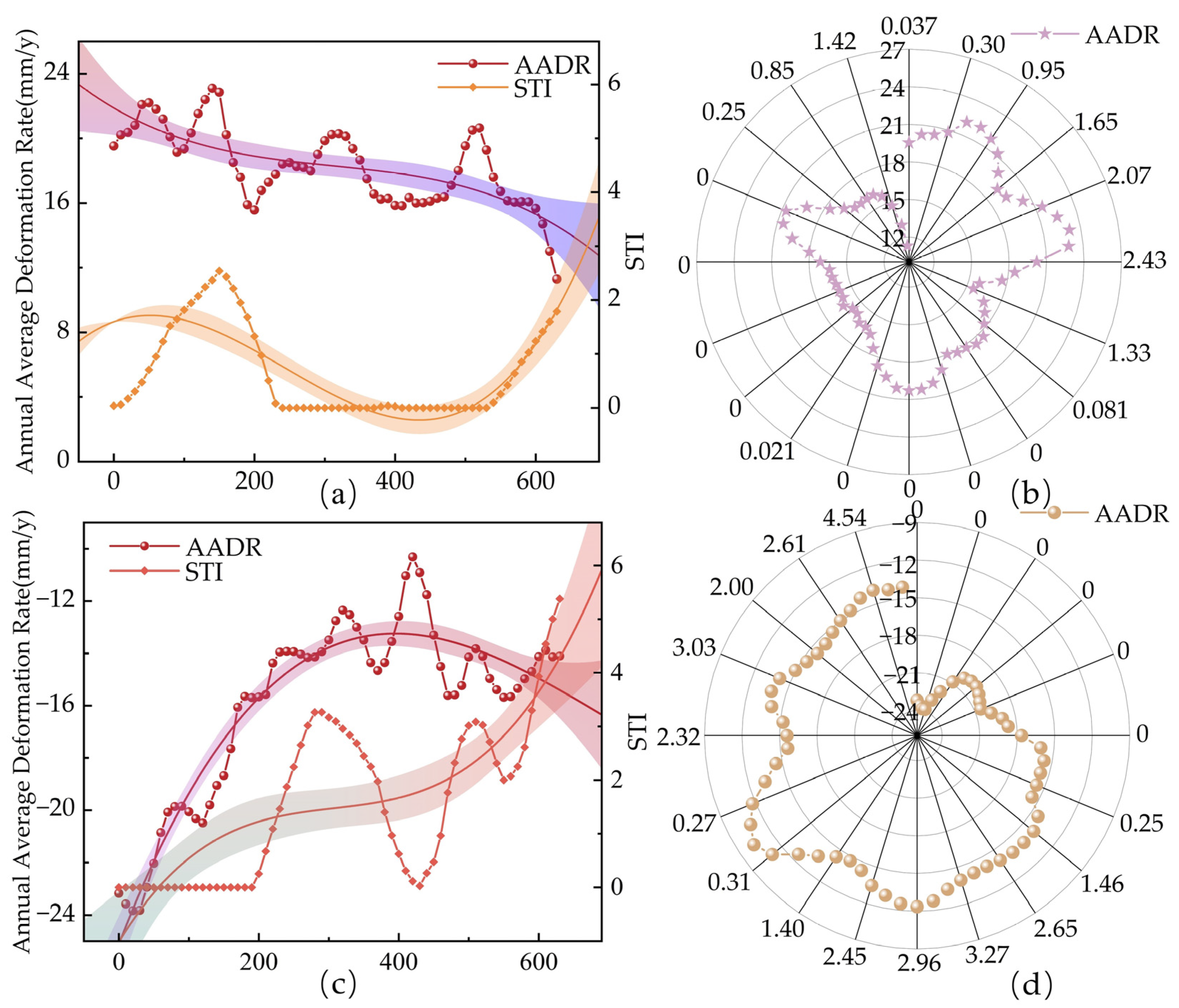
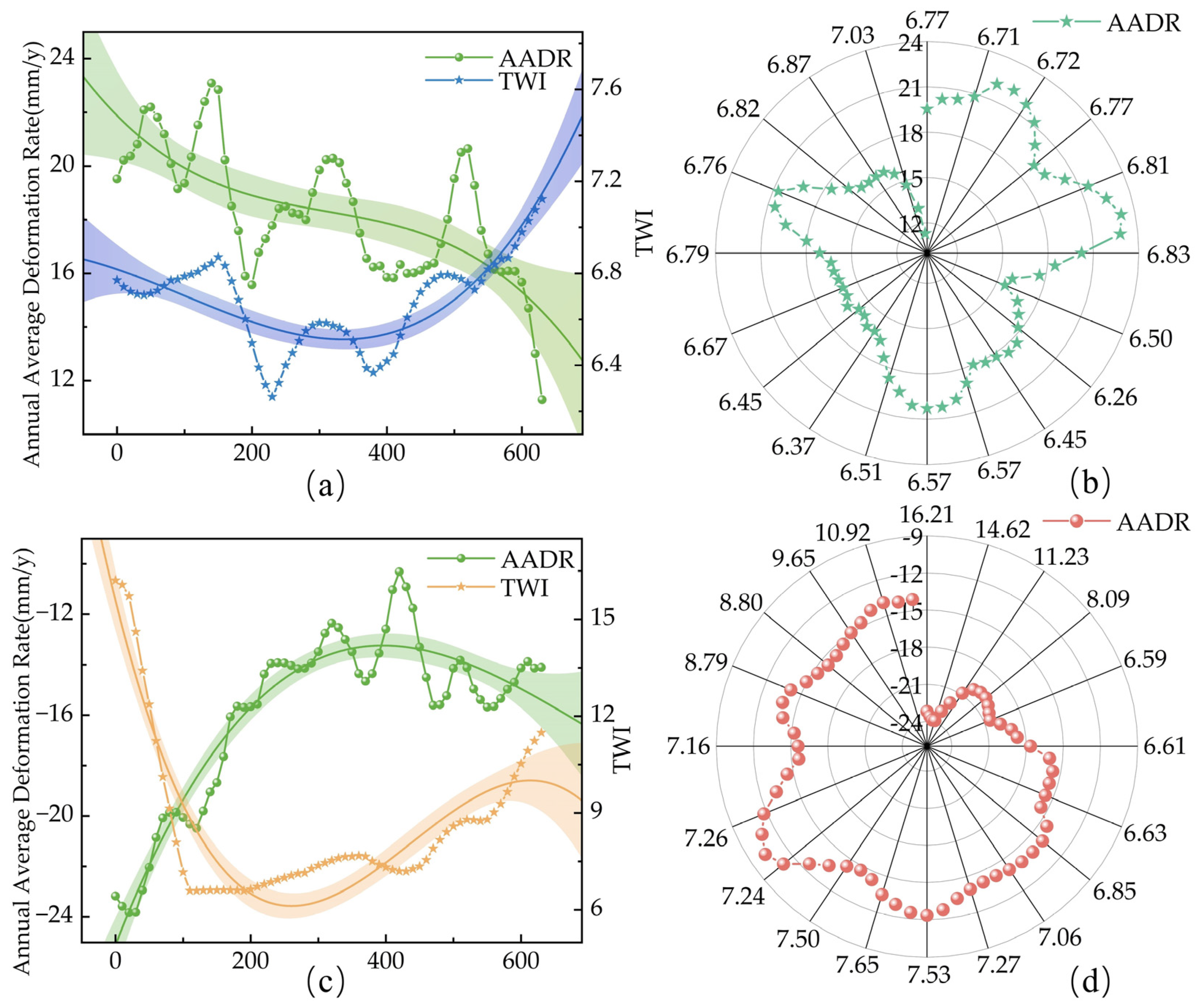
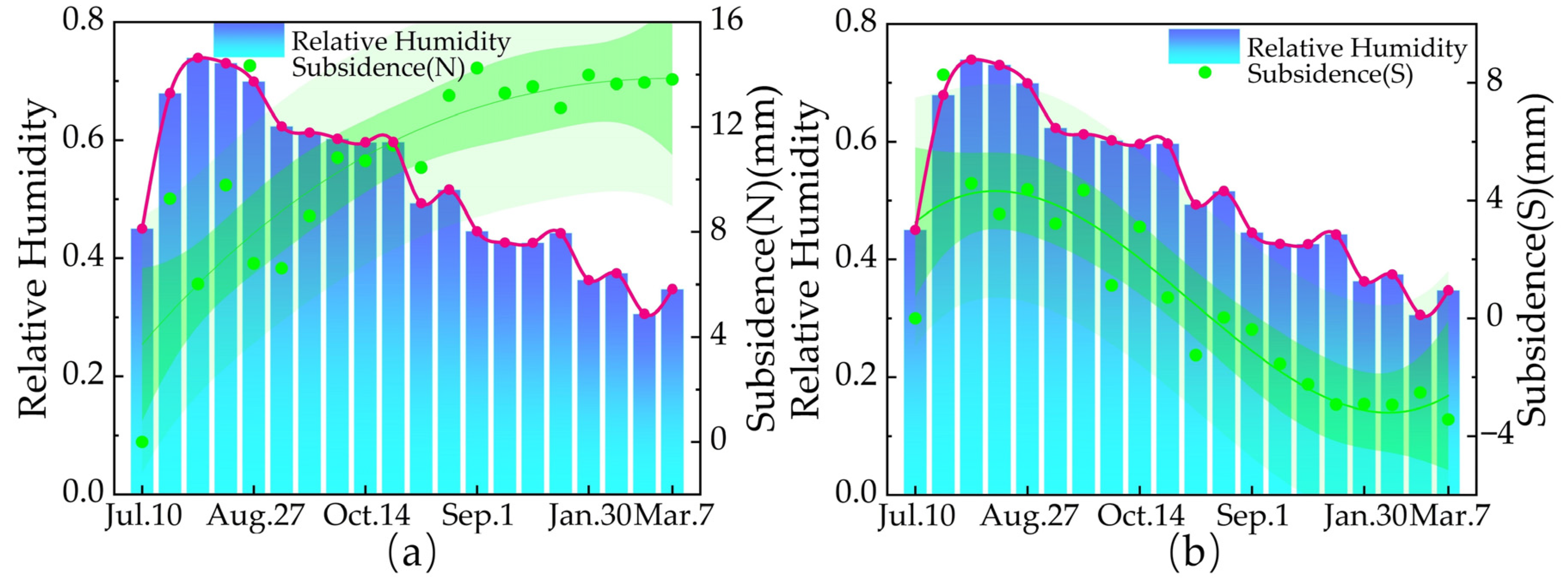
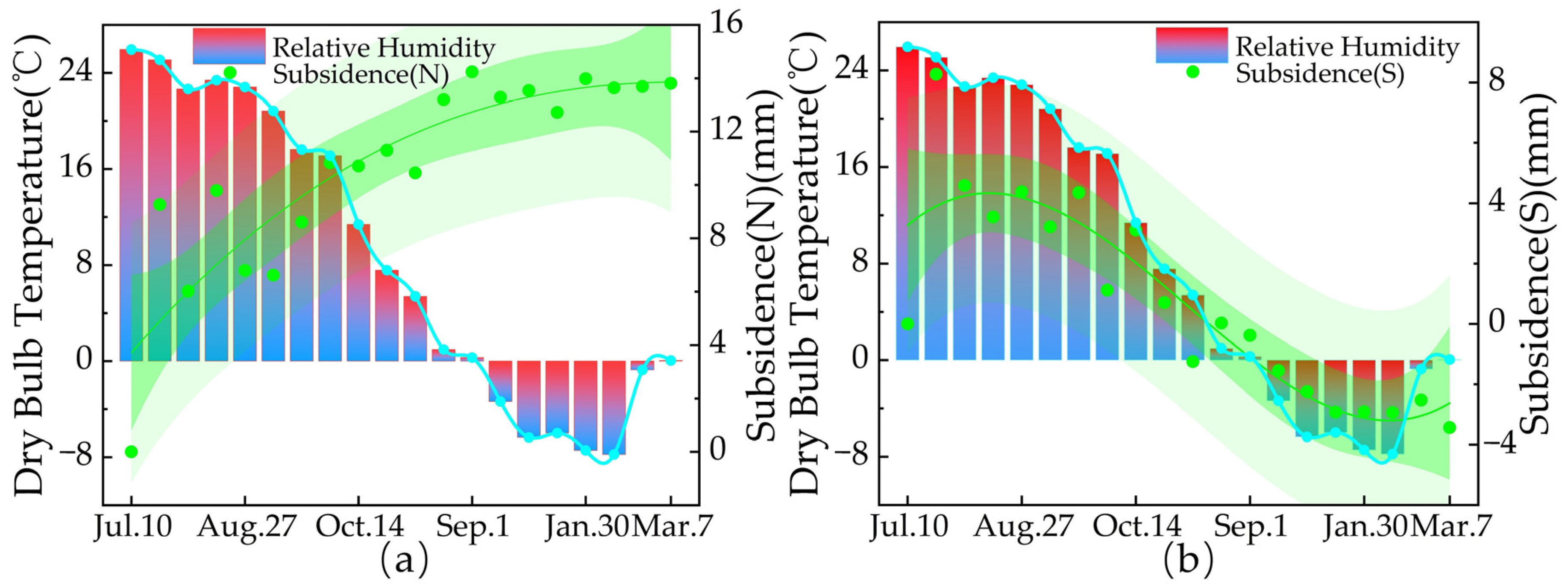
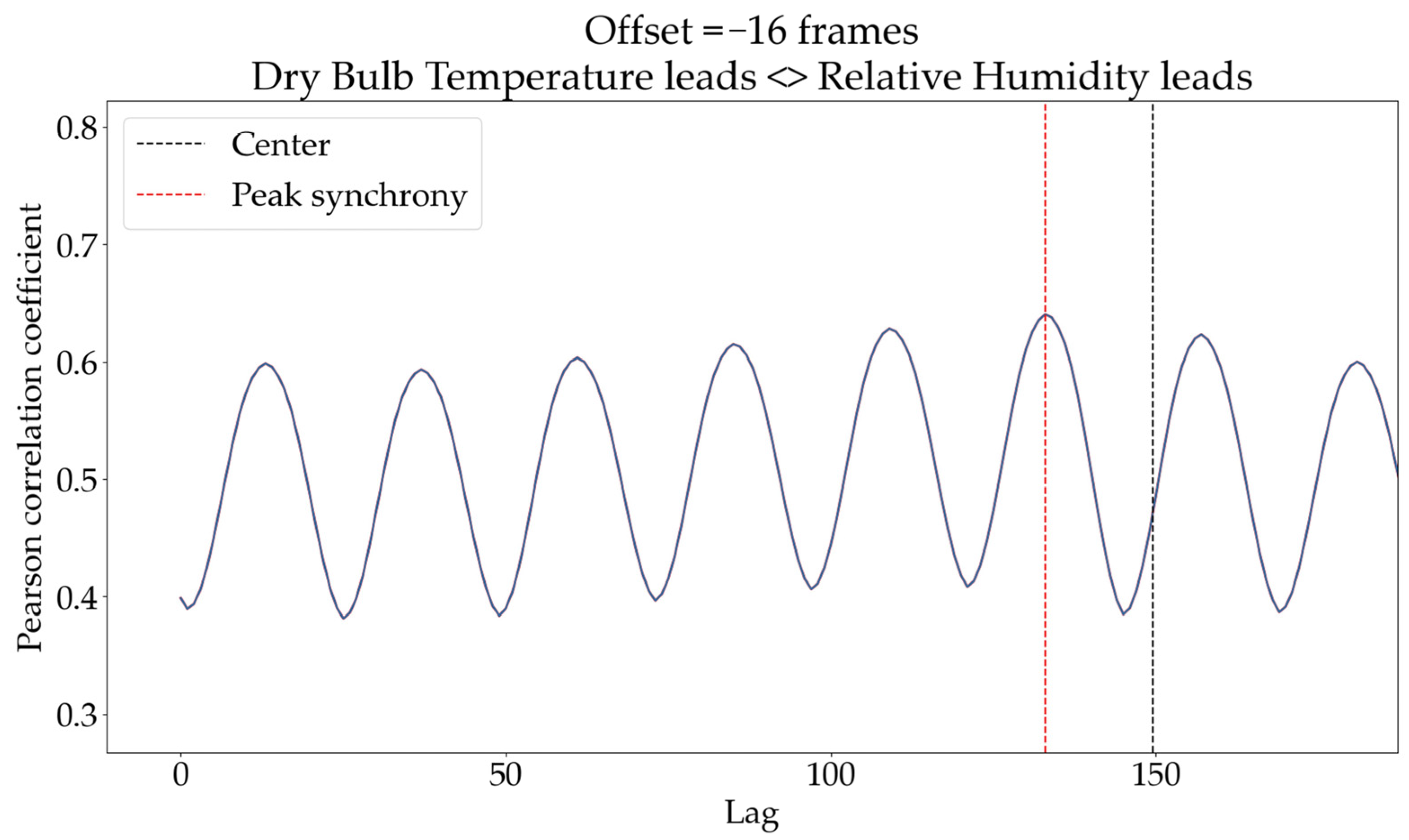

Disclaimer/Publisher’s Note: The statements, opinions and data contained in all publications are solely those of the individual author(s) and contributor(s) and not of MDPI and/or the editor(s). MDPI and/or the editor(s) disclaim responsibility for any injury to people or property resulting from any ideas, methods, instructions or products referred to in the content. |
© 2025 by the authors. Licensee MDPI, Basel, Switzerland. This article is an open access article distributed under the terms and conditions of the Creative Commons Attribution (CC BY) license (https://creativecommons.org/licenses/by/4.0/).