

Temperature Is a Key Factor Affecting Total Phosphorus and Total Nitrogen Concentrations in Northeastern Lakes Based on Sentinel-2 Images and Machine Learning Methods


 ,
,
Abstract
1. Introduction
2. Materials and Methods
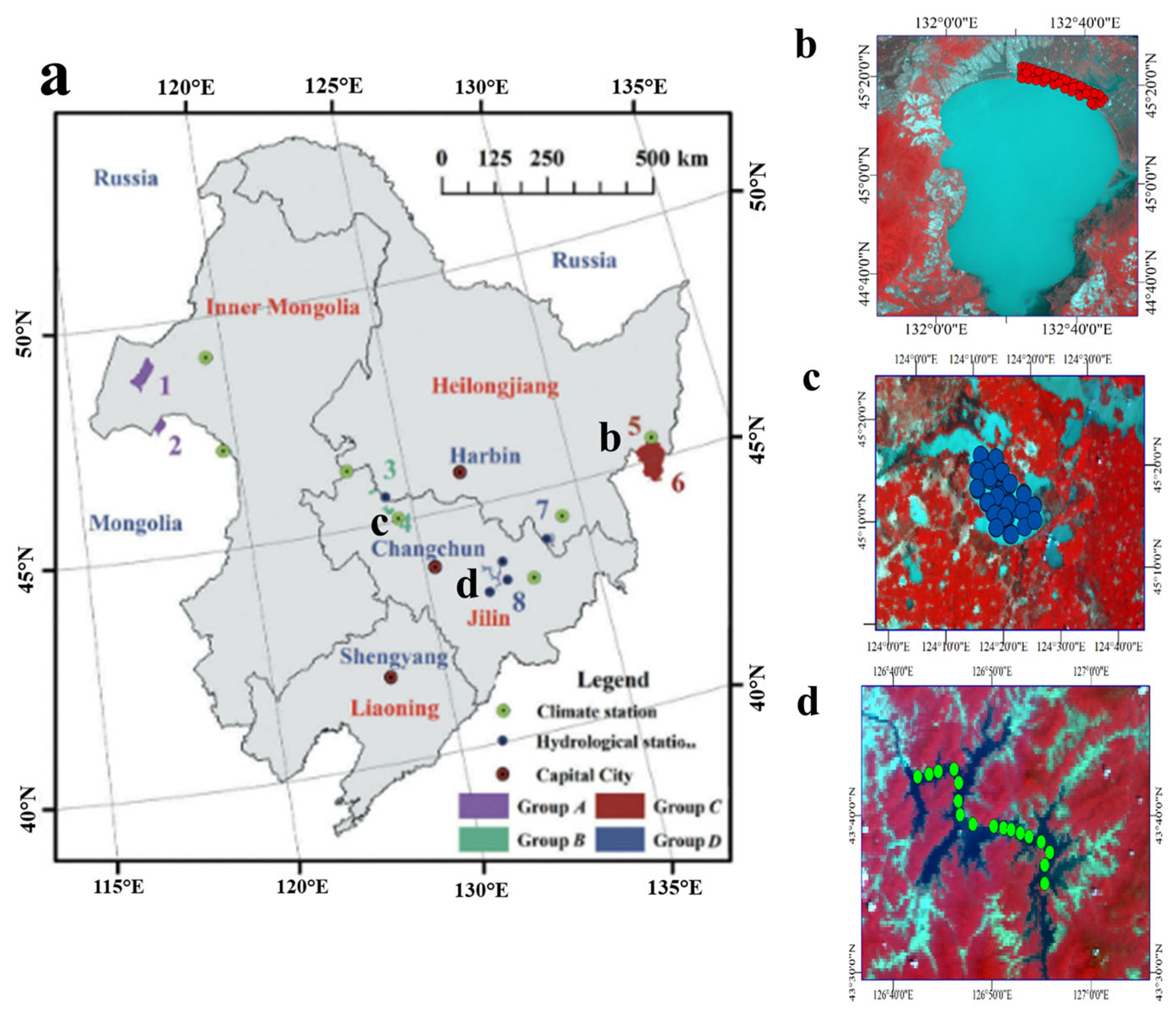
2.1. Study Area
2.2. Data Sources and Processing
2.2.1. Field Sampling and Laboratory Analysis
2.2.2. Remote Sensing Data
2.2.3. Lake Masks and Environmental Parameters
2.3. Machine Learning Methods
2.4. Statistical Analysis and Accuracy Evaluation
3. Results
3.1. Calibration and Validation of the TN and TP Algorithm
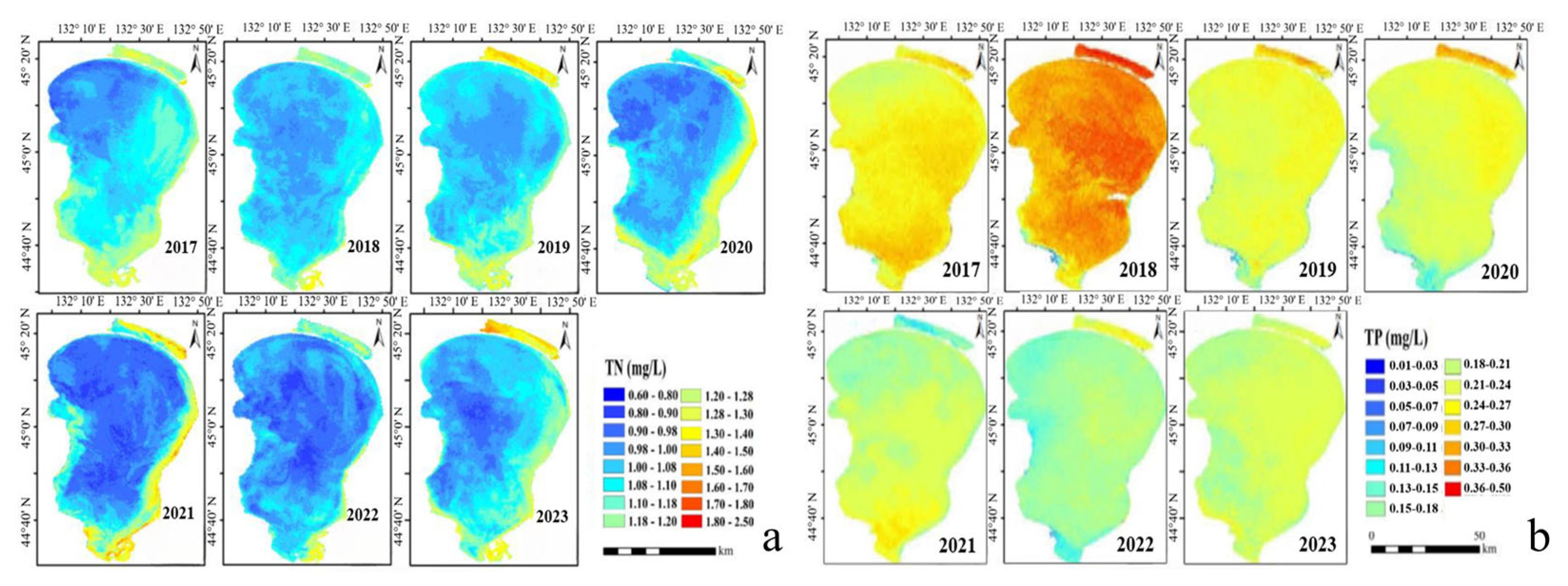
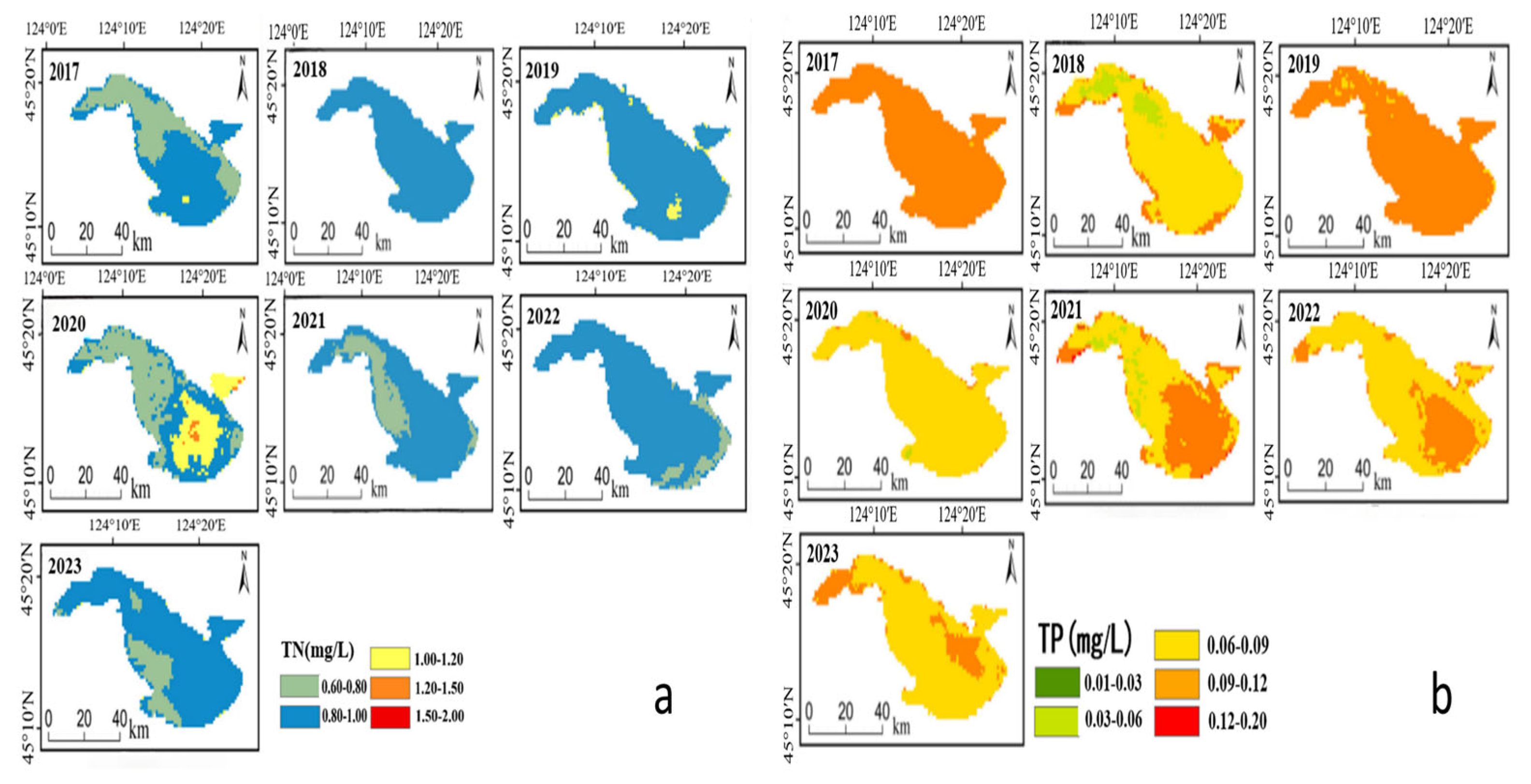
3.2. Interannual Variations in TN and TP Concentrations
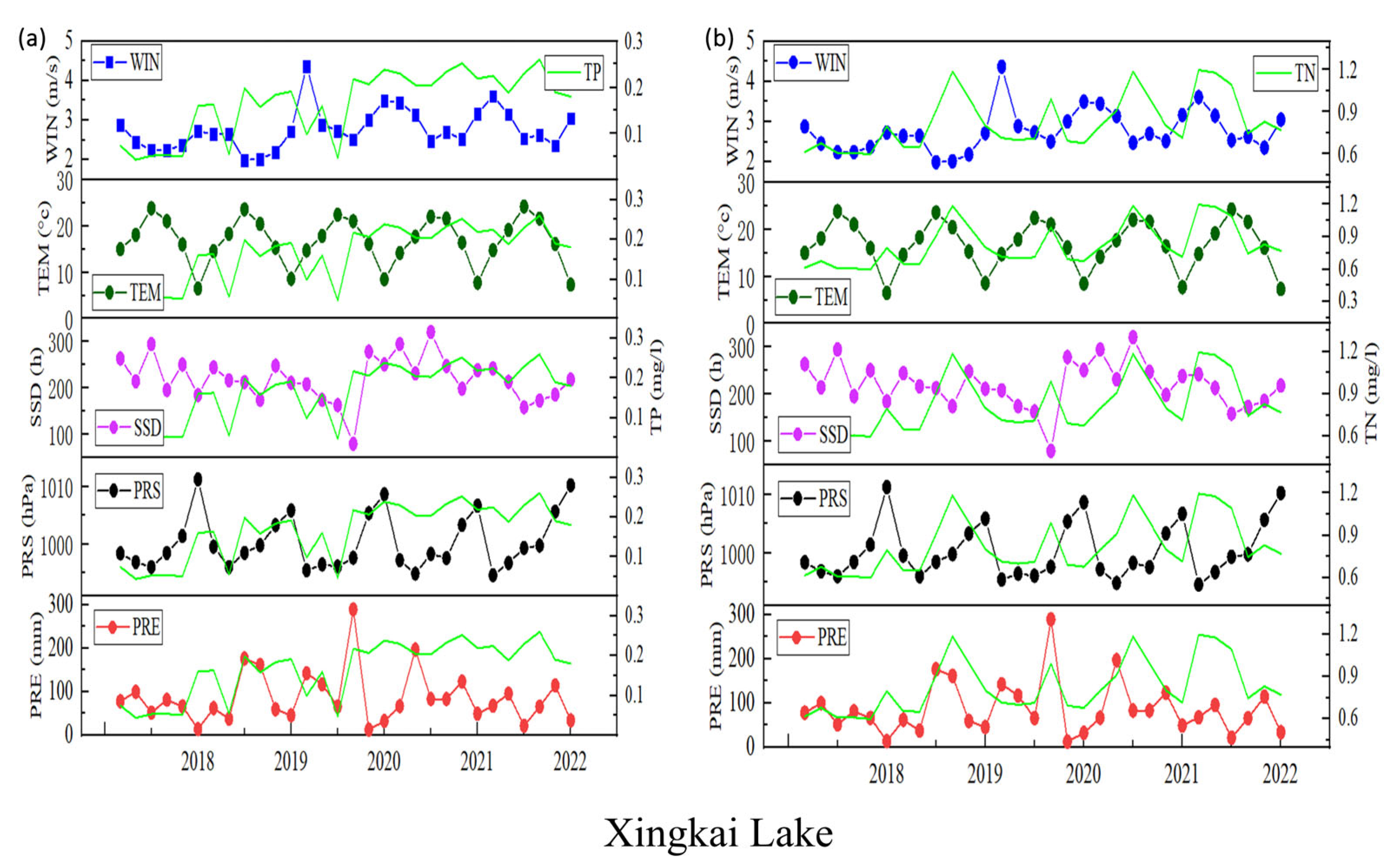
- Xingkai Lake:
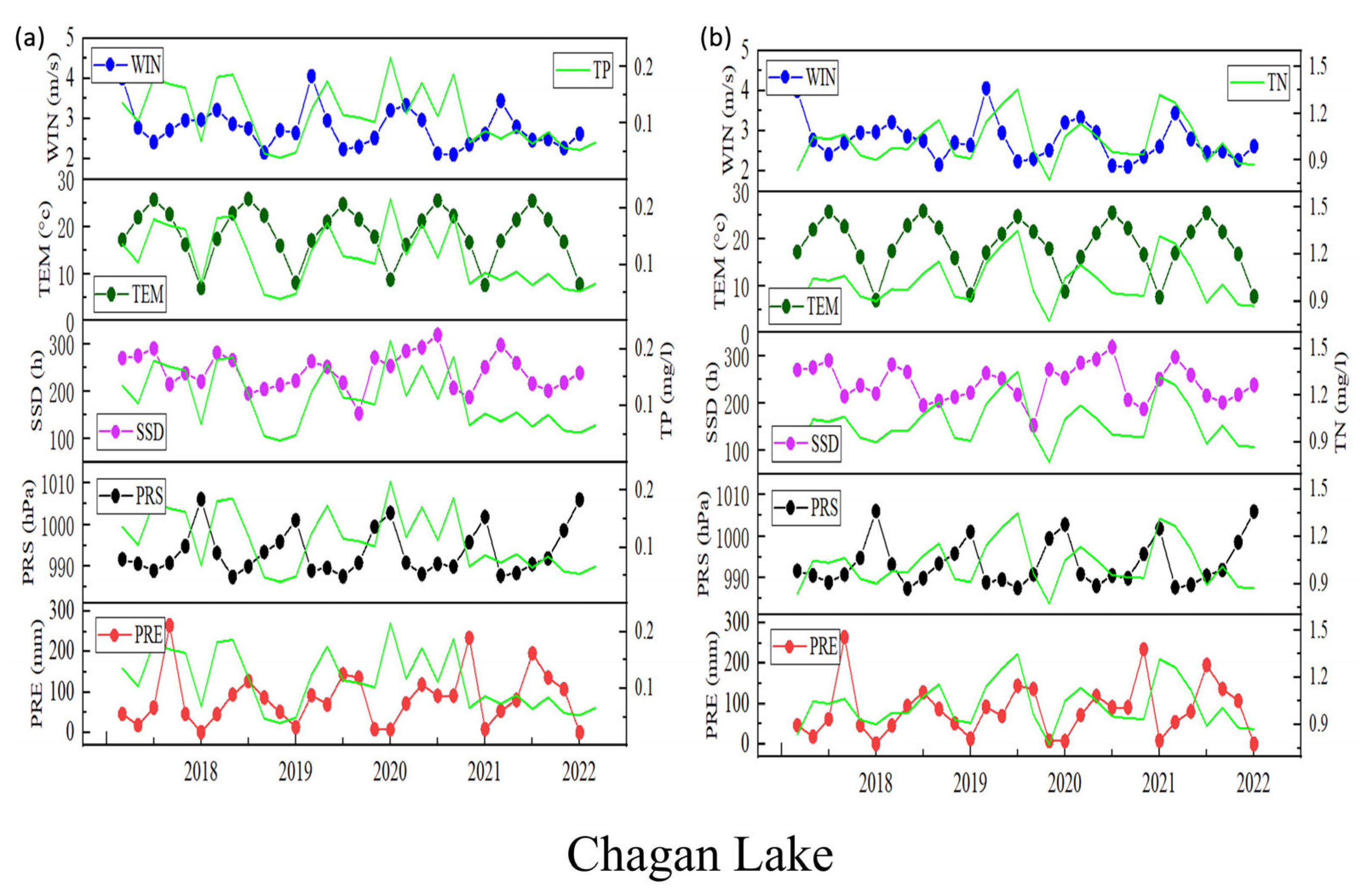
- Chagan Lake:
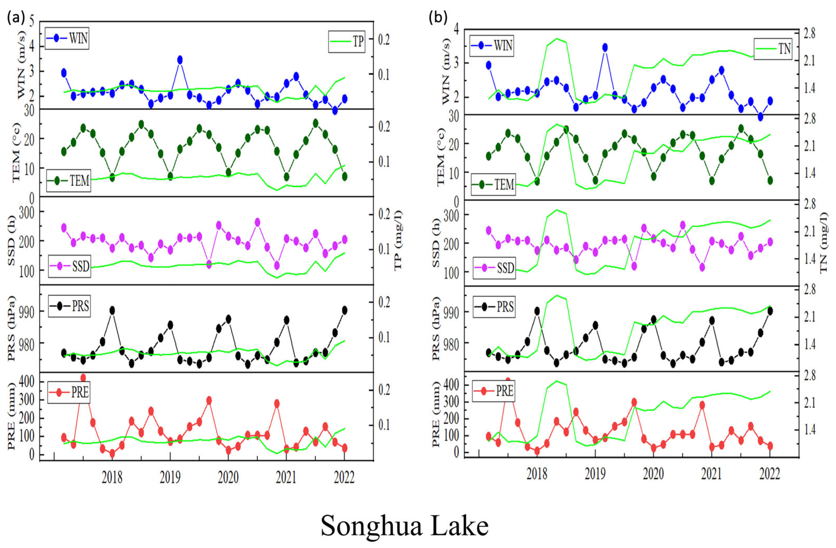
- Songhua Lake:
4. Discussion
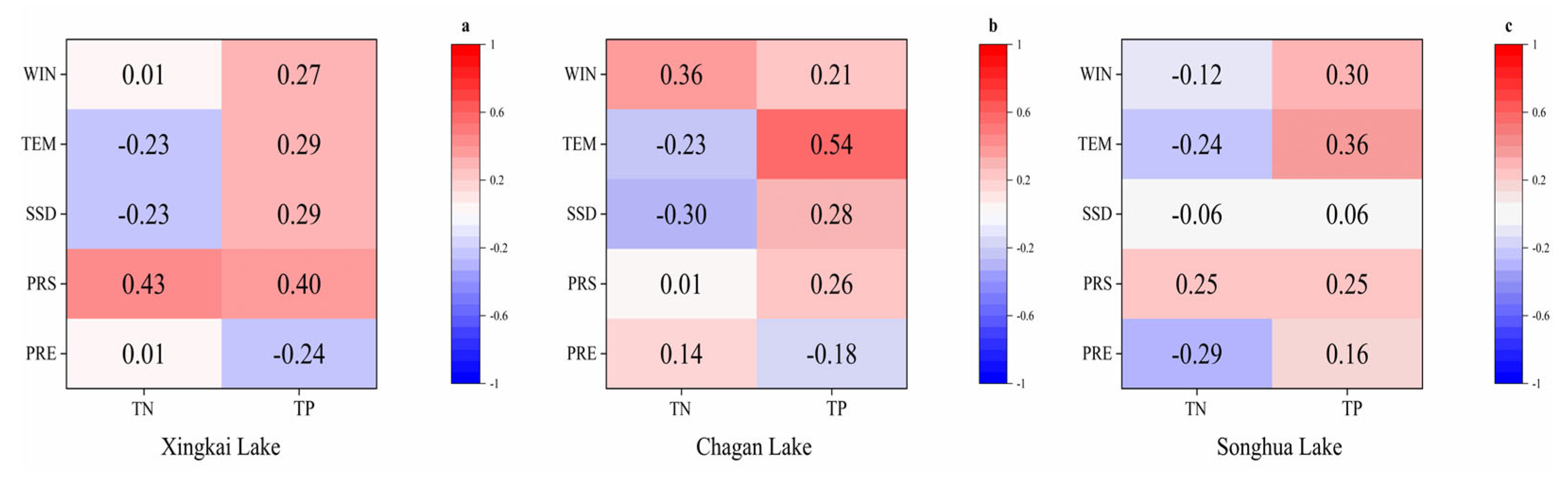
4.1. Analysis of Driving Factors
Relationship Between Meteorological Factors and TN and TP Concentrations
4.2. Applicability and Uncertainty of the Model
4.3. Implications for Environmental Management
5. Conclusions
Author Contributions
Funding
Data Availability Statement
Conflicts of Interest
References
- Ho, J.C.; Michalak, A.M.; Pahlevan, N. Widespread Global Increase in Intense Lake Phytoplankton Blooms since the 1980s. Nature 2019, 574, 667–670. [Google Scholar] [CrossRef]
- Casas-Ruiz, J.P.; Jakobsson, J.; del Giorgio, P.A. The Role of Lake Morphometry in Modulating Surface Water Carbon Concentrations in Boreal Lakes. Environ. Res. Lett. 2021, 16, 074037. [Google Scholar] [CrossRef]
- Cao, Z.; Duan, H.; Feng, L.; Ma, R.; Xue, K. Climate- and Human-Induced Changes in Suspended Particulate Matter over Lake Hongze on Short and Long Timescales. Remote Sens. Environ. 2017, 192, 98–113. [Google Scholar] [CrossRef]
- Fang, C.; Song, K.; Paerl, H.W.; Jacinthe, P.; Wen, Z.; Liu, G.; Tao, H.; Xu, X.; Kutser, T.; Wang, Z.; et al. Global Divergent Trends of Algal Blooms Detected by Satellite during 1982–2018. Glob. Change Biol. 2022, 28, 2327–2340. [Google Scholar] [CrossRef] [PubMed]
- Hou, X.; Feng, L.; Tang, J.; Song, X.-P.; Liu, J.; Zhang, Y.; Wang, J.; Xu, Y.; Dai, Y.; Zheng, Y.; et al. Anthropogenic Transformation of Yangtze Plain Freshwater Lakes: Patterns, Drivers and Impacts. Remote Sens. Environ. 2020, 248, 111998. [Google Scholar] [CrossRef]
- Fang, C. Water Quality Remote Sensing Inversion and Spatiotemporal Analysis on International Lake—A Case Study of Lake Xingkai. Ph.D. Thesis, Chinese Academy of Sciences, Changchun, China, 2020. [Google Scholar]
- Fang, C.; Song, K.; Li, L.; Wen, Z.; Liu, G.; Du, J.; Shang, Y.; Zhao, Y. Spatial Variability and Temporal Dynamics of HABs in Northeast China. Ecol. Indic. 2018, 90, 280–294. [Google Scholar] [CrossRef]
- Le, C.; Zha, Y.; Li, Y.; Sun, D.; Lu, H.; Yin, B. Eutrophication of Lake Waters in China: Cost, Causes, and Control. Environ. Manag. 2010, 45, 662–668. [Google Scholar] [CrossRef]
- Du, C.; Wang, Q.; Li, Y.; Lyu, H.; Zhu, L.; Zheng, Z.; Wen, S.; Liu, G.; Guo, Y. Estimation of Total Phosphorus Concentration Using a Water Classification Method in Inland Water. Int. J. Appl. Earth Obs. Geoinf. 2018, 71, 29–42. [Google Scholar] [CrossRef]
- Vollenweider, R. Phosphorus Loading Concept and Great Lakes Eutrophication. In Phosphorus Management Strategies for Lakes: Proceedings of the 1979 Conference Sponsored by the New York State College of Agriculture and Life Sciences, a Statutory College of the State University at Cornell University, [and] the International Joint Commission (U.S. and Canada); Ann Arbor Science: Ann Arbor, MI, USA, 1979. [Google Scholar]
- Xiong, J.; Lin, C.; Cao, Z.; Hu, M.; Xue, K.; Chen, X.; Ma, R. Development of remote sensing algorithm for total phosphorus concentration in eutrophic lakes: Conventional or machine learning? Water Res. 2022, 215, 118213. [Google Scholar] [CrossRef]
- Xiong, J.; Lin, C.; Ma, R.; Cao, Z. Remote Sensing Estimation of Lake Total Phosphorus Concentration Based on MODIS: A Case Study of Lake Hongze. Remote Sens. 2019, 11, 2068. [Google Scholar] [CrossRef]
- Gao, Y.; Gao, J.; Yin, H.; Liu, C.; Xia, T.; Wang, J.; Huang, Q. Remote Sensing Estimation of the Total Phosphorus Concentration in a Large Lake Using Band Combinations and Regional Multivariate Statistical Modeling Techniques. J. Environ. Manag. 2015, 151, 33–43. [Google Scholar] [CrossRef] [PubMed]
- Shen, M.; Duan, H.; Cao, Z.; Xue, K.; Qi, T.; Ma, J.; Liu, D.; Song, K.; Huang, C.; Song, X. Sentinel-3 OLCI Observations of Water Clarity in Large Lakes in Eastern China: Implications for SDG 6.3.2 Evaluation. Remote Sens. Environ. 2020, 247, 111950. [Google Scholar] [CrossRef]
- Sun, D.; Qiu, Z.; Li, Y.; Shi, K.; Gong, S. Detection of total phosphorus concentrations of turbid inland waters using a remote sensing method. Water Air Soil Pollut. 2014, 225, 1953. [Google Scholar] [CrossRef]
- Cai, X.; Li, Y.; Lei, S.; Zeng, S.; Zhao, Z.; Lyu, H.; Dong, X.; Li, J.; Wang, H.; Xu, J.; et al. A Hybrid Remote Sensing Approach for Estimating Chemical Oxygen Demand Concentration in Optically Complex Waters: A Case Study in Inland Lake Waters in Eastern China. Sci. Total Environ. 2023, 856, 158869. [Google Scholar] [CrossRef]
- Wimmer, A.; Markus, A.A.; Schuster, M. Silver Nanoparticle Levels in River Water: Real Environmental Measurements and Modeling Approaches—A Comparative Study. Environ. Sci. Technol. Lett. 2019, 6, 353–358. [Google Scholar] [CrossRef]
- Chang, N.-B.; Xuan, Z.; Yang, Y.J. Exploring Spatiotemporal Patterns of Phosphorus Concentrations in a Coastal Bay with MODIS Images and Machine Learning Models. Remote Sens. Environ. 2013, 134, 100–110. [Google Scholar] [CrossRef]
- Wang, J.; Cheng, S.; Jia, H.; Wang, Z.; Tang, U.W. An artificial neural network model for lake color inversion using TM imagery. Huan Jing Ke Xue 2003, 24, 73–76. [Google Scholar]
- Chen, J.; Quan, W.; Cui, T.; Song, Q.; Lin, C. Remote Sensing of Absorption and Scattering Coefficient Using Neural Network Model: Development, Validation, and Application. Remote Sens. Environ. 2014, 149, 213–226. [Google Scholar] [CrossRef]
- Concha, J.A.; Schott, J.R. Retrieval of Color Producing Agents in Case 2 Waters Using Landsat 8. Remote Sens. Environ. 2016, 185, 95–107. [Google Scholar] [CrossRef]
- Boateng, E.Y.; Otoo, J.; Abaye, D.A. Basic Tenets of Classification Algorithms K-Nearest-Neighbor, Support Vector Machine, Random Forest and Neural Network: A Review. J. Data Anal. Inf. Process. 2020, 8, 341–357. [Google Scholar] [CrossRef]
- Hearst, M.A.; Dumais, S.T.; Osuna, E.; Platt, J.; Scholkopf, B. Support Vector Machines. IEEE Intell. Syst. Their Appl. 1998, 13, 18–28. [Google Scholar] [CrossRef]
- Cervantes, J.; Garcia-Lamont, F.; Rodríguez-Mazahua, L.; Lopez, A. A Comprehensive Survey on Support Vector Machine Classification: Applications, Challenges and Trends. Neurocomputing 2020, 408, 189–215. [Google Scholar] [CrossRef]
- Sheykhmousa, M.; Mahdianpari, M.; Ghanbari, H.; Mohammadimanesh, F.; Ghamisi, P.; Homayouni, S. Support Vector Machine Versus Random Forest for Remote Sensing Image Classification: A Meta-Analysis and Systematic Review. IEEE J. Sel. Top. Appl. Earth Obs. Remote Sens. 2020, 13, 6308–6325. [Google Scholar] [CrossRef]
- Li, X.; Ding, J.; Ilyas, N. Machine Learning Method for Quick Identification of Water Quality Index (WQI) Based on Sentinel-2 MSI Data: Ebinur Lake Case Study. Water Supply 2021, 21, 1291–1312. [Google Scholar] [CrossRef]
- Belgiu, M.; Drăguţ, L. Random Forest in Remote Sensing: A Review of Applications and Future Directions. ISPRS J. Photogramm. Remote Sens. 2016, 114, 24–31. [Google Scholar] [CrossRef]
- Xu, S.; Li, S.; Tao, Z.; Song, K.; Wen, Z.; Li, Y.; Chen, F. Remote Sensing of Chlorophyll-a in Xinkai Lake Using Machine Learning and GF-6 WFV Images. Remote Sens. 2022, 14, 5136. [Google Scholar] [CrossRef]
- Qiang, S.; Song, K.; Shang, Y.; Lai, F.; Wen, Z.; Liu, G.; Tao, H.; Lyu, Y. Remote Sensing Estimation of CDOM and DOC with the Environmental Implications for Lake Khanka. Remote Sens. 2023, 15, 5707. [Google Scholar] [CrossRef]
- Shi, X.; Gu, L.; Jiang, T.; Zheng, X.; Dong, W.; Tao, Z. Retrieval of Chlorophyll-a Concentrations Using Sentinel-2 MSI Imagery in Lake Chagan Based on Assessments with Machine Learning Models. Remote Sens. 2022, 14, 4924. [Google Scholar] [CrossRef]
- Ji, X.; Liu, T.; Liu, J.; Li, J.; Pan, B. Investigation and Study on Water Quality and Pollution Condition in Lake Xingkai of China. Environ. Monit. China 2013, 29, 79–84. [Google Scholar]
- Sun, D.; Sun, X. Hydrological Characteristics of Xingkai Lake. Water Resour. Hydropower Northeast China 2006, 24, 21. [Google Scholar]
- Zhu, L.; Yan, B.; Wang, L.; Pan, X. Mercury Concentration in the Muscle of Seven Fish Species from Chagan Lake, Northeast China. Environ. Monit. Assess. 2012, 184, 1299–1310. [Google Scholar] [CrossRef] [PubMed]
- Water quality Determination of Phosphate and Total Phosphorus Continuous Flow—Ammonium Molybdate Spectrophotometric mMethod. Available online: https://www.mee.gov.cn/ywgz/fgbz/bz/bzwb/jcffbz/201311/t20131106_262958.shtml (accessed on 19 December 2024).
- Liang, Y.; Yin, F.; Xie, D.; Liu, L.; Zhang, Y.; Ashraf, T. Inversion and Monitoring of the TP Concentration in Taihu Lake Using the Landsat-8 and Sentinel-2 Images. Remote Sens. 2022, 14, 6284. [Google Scholar] [CrossRef]
- Orusa, T.; Viani, A.; Cammareri, D.; Borgogno Mondino, E. A Google Earth Engine Algorithm to Map Phenological Metrics in Mountain Areas Worldwide with Landsat Collection and Sentinel-2. Geomatics 2023, 3, 221–238. [Google Scholar] [CrossRef]
- Long, X.; Li, X.; Lin, H.; Zhang, M. Mapping the Vegetation Distribution and Dynamics of a Wetland Using Adaptive-Stacking and Google Earth Engine Based on Multi-Source Remote Sensing Data. Int. J. Appl. Earth Obs. Geoinf. 2021, 102, 102453. [Google Scholar] [CrossRef]
- Gao, B. NDWI—A Normalized Difference Water Index for Remote Sensing of Vegetation Liquid Water from Space. Remote Sens. Environ. 1996, 58, 257–266. [Google Scholar] [CrossRef]
- Rouse, J.W.; Haas, R.H.; Schell, J.A.; Deering, D.W. Monitoring Vegetation Systems in the Great Plains with ERTS. NASA Spec. Publ. 1974, 351, 309. [Google Scholar]
- Breiman, L. Random Forests. Mach. Learn. 2001, 45, 5–32. [Google Scholar] [CrossRef]
- Behrouz, M.S.; Yazdi, M.N.; Sample, D.J. Using Random Forest, a Machine Learning Approach to Predict Nitrogen, Phosphorus, and Sediment Event Mean Concentrations in Urban Runoff. J. Environ. Manag. 2022, 317, 115412. [Google Scholar] [CrossRef]
- Fang, C.; Song, C.; Wang, X.; Wang, Q.; Tao, H.; Wang, X.; Ma, Y.; Song, K. A Novel Total Phosphorus Concentration Retrieval Method Based on Two-Line Classification in Lakes and Reservoirs across China. Sci. Total Environ. 2024, 906, 167522. [Google Scholar] [CrossRef]
- Chen, T.; Guestrin, C. XGBoost: A Scalable Tree Boosting System. In Proceedings of the 22nd ACM SIGKDD International Conference on Knowledge Discovery and Data Mining, New York, NY, USA, 13 August 2016; pp. 785–794. [Google Scholar]
- Ramraj, S.; Uzir, N.; Sunil, R.; Banerjee, S. Experimenting XGBoost Algorithm for Prediction and Classification of Different Datasets. Int. J. Control Theory Appl. 2016, 9, 651–662. [Google Scholar]
- Cao, Z.; Ma, R.; Duan, H.; Pahlevan, N.; Melack, J.; Shen, M.; Xue, K. A Machine Learning Approach to Estimate Chlorophyll-a from Landsat-8 Measurements in Inland Lakes. Remote Sens. Environ. 2020, 248, 111974. [Google Scholar] [CrossRef]
- Peterson, K.T.; Sagan, V.; Sidike, P.; Hasenmueller, E.A.; Sloan, J.J.; Knouft, J.H. Machine Learning-Based Ensemble Prediction of Water-Quality Variables Using Feature-Level and Decision-Level Fusion with Proximal Remote Sensing. Photogramm. Eng. Remote Sens. 2019, 85, 269–280. [Google Scholar] [CrossRef]
- Shang, W.; Jin, S.; He, Y.; Zhang, Y.; Li, J. Spatial–Temporal Variations of Total Nitrogen and Phosphorus in Poyang, Dongting and Taihu Lakes from Landsat-8 Data. Water 2021, 13, 1704. [Google Scholar] [CrossRef]
- McQueen, D.J.; Lean, D.R.S.; McQueen, D.J.; Lean, D.R.S. Influence of Water Temperature and Nitrogen to Phosphorus Ratios on the Dominance of Blue-Green Algae in Lake St. George, Ontario. Can. J. Fish. Aquat. Sci. 1987, 44, 598–604. [Google Scholar] [CrossRef]
- Lu, Y.; Li, S.; Zuo, L.; Liu, H.; Roelvink, J. Advances in Sediment Transport under Combined Action of Waves and Currents. Int. J. Sediment. Res. 2015, 30, 351–360. [Google Scholar] [CrossRef]
- Lian, H.-S.; Liu, H.-B.; Li, X.-D.; Song, T.; Liu, S.; Lei, Q.-L.; Ren, T.-Z.; Wu, S.-X.; Li, Y. Characteristics of Nitrogen Variation and Its Response to Rainfall: A Case Study in Wuxi Port at Taihu Lake Basin. Huan Jing Ke Xue Huanjing Kexue 2017, 38, 5047–5055. [Google Scholar]
- Sinha, E.; Michalak, A.M. Precipitation Dominates Interannual Variability of Riverine Nitrogen Loading across the Continental United States. Environ. Sci. Technol. 2016, 50, 12874–12884. [Google Scholar] [CrossRef]
- Gallo, E.L.; Meixner, T.; Aoubid, H.; Lohse, K.A.; Brooks, P.D. Combined Impact of Catchment Size, Land Cover, and Precipitation on Streamflow and Total Dissolved Nitrogen: A Global Comparative Analysis. Glob. Biogeochem. Cycles 2015, 29, 1109–1121. [Google Scholar] [CrossRef]
- Henson, S.A.; Cael, B.B.; Allen, S.R.; Dutkiewicz, S. Future Phytoplankton Diversity in a Changing Climate. Nat. Commun. 2021, 12, 5372. [Google Scholar] [CrossRef]
- Winder, M.; Sommer, U. Phytoplankton Response to a Changing Climate. Hydrobiologia 2012, 698, 5–16. [Google Scholar] [CrossRef]
- Podsetchine, V.; Schernewski, G. The Influence of Spatial Wind Inhomogeneity on Flow Patterns in a Small Lake. Water Res. 1999, 33, 3348–3356. [Google Scholar] [CrossRef]
- Zhang, Y.; Shen, F.; Sun, X.; Tan, K. Marine Big Data-Driven Ensemble Learning for Estimating Global Phytoplankton Group Composition over Two Decades (1997–2020). Remote Sens. Environ. 2023, 294, 113596. [Google Scholar] [CrossRef]
- Kelepertzis, E.; Argyraki, A.; Daftsis, E. Geochemical Signature of Surface Water and Stream Sediments of a Mineralized Drainage Basin at NE Chalkidiki, Greece: A Pre-Mining Survey. J. Geochem. Explor. 2012, 114, 70–81. [Google Scholar] [CrossRef]
- Shi, K.; Zhang, Y.; Zhang, Y.; Li, N.; Qin, B.; Zhu, G.; Zhou, Y. Phenology of Phytoplankton Blooms in a Trophic Lake Observed from Long-Term MODIS Data. Environ. Sci. Technol. 2019, 53, 2324–2331. [Google Scholar] [CrossRef]
- van Wijk, D.; Janse, J.H.; Wang, M.; Kroeze, C.; Mooij, W.M.; Janssen, A.B.G. How Nutrient Retention and TN:TP Ratios Depend on Ecosystem State in Thousands of Chinese Lakes. Sci. Total Environ. 2024, 918, 170690. [Google Scholar] [CrossRef]
- Sinha, E.; Michalak, A.M.; Balaji, V. Eutrophication Will Increase during the 21st Century as a Result of Precipitation Changes. Science 2017, 357, 405–408. [Google Scholar] [CrossRef]


| Number | Date | Songhua Lake | Xingkai Lake | Chagan Lake | TP | TN |
|---|---|---|---|---|---|---|
| 1 | 18 August 2021 | 10 | 10 | 10 | ||
| 2 | 1 September 2021 | 20 | 20 | 20 | ||
| 3 | 17 September 2021 | 19 | 19 | 19 | ||
| 4 | 28 September 2021 | 9 | 9 | 9 | ||
| 5 | 11 October 2021 | 18 | 18 | 18 | ||
| 6 | 22 October 2021 | 19 | 19 | 19 | ||
| 7 | 23 October 2021 | 18 | 18 | 18 | ||
| 8 | 21 September 2022 | 18 | 18 | 18 | ||
| Total | 18 | 65 | 48 |
| Spectral Band | TN | TP |
|---|---|---|
| Basic Bands | B1, B6, B7, B8 | B3, B6, B8, B8A |
| Band Combinations | B1 − B6, B1 − B8, (B1 − B6)/(B1 + B6), B1 − B7, B1 − B4, (B1 − B4)/(B1 + B4), (B1 − B7)/(B1 + B7), B1 − B5 | B8 − B8A, B6 − B8A, (B5 + B8)/(B5 − B8), (B5 + B6)/(B5 − B6), B5/B5 − B8, B5/B5 − B6, (B3 + B8A)/(B3 − B8A) |
Disclaimer/Publisher’s Note: The statements, opinions and data contained in all publications are solely those of the individual author(s) and contributor(s) and not of MDPI and/or the editor(s). MDPI and/or the editor(s) disclaim responsibility for any injury to people or property resulting from any ideas, methods, instructions or products referred to in the content. |
© 2025 by the authors. Licensee MDPI, Basel, Switzerland. This article is an open access article distributed under the terms and conditions of the Creative Commons Attribution (CC BY) license (https://creativecommons.org/licenses/by/4.0/).
Share and Cite
Qin, H.; Fang, C.; Liu, G.; Song, K.; Li, Z.; Li, S.; Tao, H.; Yan, Z. Temperature Is a Key Factor Affecting Total Phosphorus and Total Nitrogen Concentrations in Northeastern Lakes Based on Sentinel-2 Images and Machine Learning Methods. Remote Sens. 2025, 17, 267. https://doi.org/10.3390/rs17020267
Qin H, Fang C, Liu G, Song K, Li Z, Li S, Tao H, Yan Z. Temperature Is a Key Factor Affecting Total Phosphorus and Total Nitrogen Concentrations in Northeastern Lakes Based on Sentinel-2 Images and Machine Learning Methods. Remote Sensing. 2025; 17(2):267. https://doi.org/10.3390/rs17020267
Chicago/Turabian StyleQin, Haoming, Chong Fang, Ge Liu, Kaishan Song, Zhuoshi Li, Sijia Li, Hui Tao, and Zhaojiang Yan. 2025. "Temperature Is a Key Factor Affecting Total Phosphorus and Total Nitrogen Concentrations in Northeastern Lakes Based on Sentinel-2 Images and Machine Learning Methods" Remote Sensing 17, no. 2: 267. https://doi.org/10.3390/rs17020267
APA StyleQin, H., Fang, C., Liu, G., Song, K., Li, Z., Li, S., Tao, H., & Yan, Z. (2025). Temperature Is a Key Factor Affecting Total Phosphorus and Total Nitrogen Concentrations in Northeastern Lakes Based on Sentinel-2 Images and Machine Learning Methods. Remote Sensing, 17(2), 267. https://doi.org/10.3390/rs17020267