Inclined Aerial Image and Satellite Image Matching Based on Edge Curve Direction Angle Features

Abstract

Optical remote sensing images are easily affected by atmospheric absorption and scattering, and the low contrast and low signal-to-noise ratio (SNR) of aerial images as well as the different sensors of aerial and satellite images bring a great challenge to image matching. A tilted aerial image and satellite image matching algorithm based on edge curve direction angle features (ECDAF) is proposed, which accomplishes image matching by extracting the edge features of the images and establishing the curve direction angle feature descriptors. First, tilt and resolution transforms are performed on the satellite image, and edge detection and contour extraction are performed on the aerial image and transformed satellite image to make preparations for image matching. Then, corner points are detected and feature descriptors are constructed based on the edge curve direction angle. Finally, the integrated matching similarity is computed to realize aerial–satellite image matching. Experiments run on a variety of remote sensing datasets including forests, hills, farmland, and lake scenes demonstrate that the effectiveness of the proposed algorithm shows a great improvement over existing state-of-the-art algorithms.

1. Introduction

Image matching is the process of finding the same point in two or more images of the same scene [1,2,3]. Optical remote sensing images may be taken by different sensors under different shooting angles, distances, light conditions, and atmospheric visibilities [4,5]. Tilted aerial image and satellite image matching is of great importance and is a prerequisite for a variety of visual tasks, such as image fusion, image mosaicking, target localization, and image retrieval [6,7]. Image matching methods are mainly divided into two categories: feature-driven matching methods and data-driven matching methods. Feature-driven methods realize image matching by extracting the common features of two or more images [8], and data-driven methods mainly refer to image matching methods based on deep learning [9].

Point feature matching belongs to the category of feature-driven image matching methods [10,11]. Lowe [12] proposed the SIFT operator, which is invariant to scale, rotation, and illumination change. The SIFT algorithm is implemented in the Gaussian difference pyramid to achieve keypoints detection, and then feature matching is achieved by computing the gradient distribution around the keypoints [13]. Considering the feature points detection speed, Bay and others put forward the SURF [14] method. The SURF operator is obtained by searching the extreme value of determinant of Hessian in scale space, and the concepts of integral images and box filters are used in the process of feature detection. The Harris operator [15] is computed by Taylor’s formula, which makes the operator insensitive to illumination change. The Fast operator [16] is proposed based on machine learning and carries out feature points matching by constructing a decision tree. The BRIEF operator [17] needs to detect the feature points with the help of other matching operators, and binary strings are used as an efficient feature point descriptor. The ORB operator [18] detects the feature points using the FAST algorithm and then describes the feature points using the improved BRIEF operator. Yu and Morel [19] proposed the ASIFT operator with affine invariance. The ASIFT algorithm abstracts the viewpoint changes caused by camera and scene motion into a simplified spatial imaging model. It transforms the perspective of the image at different azimuth and pitch angles, and then feature matching is carried out using the SIFT operator. The ASIFT method is more effective in matching images under large viewpoint changes. Point feature matching is easily affected by noise and low contrast, and it is less effective for long-distance remote sensing images.

Line feature matching also belongs to the category of feature-driven image matching methods. Because line features can better reflect the structural information of the scene, they have received a lot of attention from researchers. Line feature matching methods include single-line feature matching methods, multi-line feature matching methods, and point-line feature matching methods. Single-line feature matching methods utilize the local appearance or geometric attributes of single line segments to achieve image matching. Wang and others [20] proposed a mean standard deviation line descriptor (MSLD) for straight line segment matching. A line gradient description matrix (GDM) is formed for the pixel support region (PSR), and then the mean and standard deviation of GDM column vectors are computed to obtain the MSLD. The MSLD descriptor is highly distinctive for line matching under noise, illumination change, viewpoint change, and rotation. A line band descriptor (LBD) [21] which contains the gradient features of the local region of a line was proposed. The LBD method utilizes both the geometric attributes of lines and their local appearance to improve the matching accuracy. Multi-line feature matching methods can obtain additional geometric structure information. Wang and others [22] put forward a wide-baseline image matching approach based on multi-line features. Line segments are clustered into local groups according to spatial proximity. The length ratio, the angle, and the average gradient magnitude of the two line segments are computed as the line descriptor, and this shows improved results with low-texture scenes. López et al. [23] proposed a matching method based on the structural information of neighboring line segments, which utilizes a phase-based edge detector to perform line detection over Gaussian scale-space. Point-line feature matching methods have also received extensive attention from researchers. Lourakis et al. [24] utilized a randomized search strategy combined with the two-line two-point projective invariant to achieve points and lines matching. Fan and others [25] utilized line-point invariants constituted by a line and its neighboring points to achieve line matching. Two kinds of line-point invariants were introduced, of which one is an affine invariant consisting of one line and two points while the other is a projective invariant consisting of one line and four points. Line feature matching is susceptible to line segment fragmentation and is not ideal for matching remote sensing images at long distances.

Deep learning image matching methods belong to the category of data-driven image matching methods. By building models from a large amount of training data and learning pixel-level matching relationships from similar structural information, deep learning image matching algorithms have superior feature expression capabilities [26,27,28]. Image matching networks can be classified into two categories. One aims to replace part of the image matching steps by building a deep neural network, which is called a single-step matching network. The other aims to complete the whole image matching process by building a deep neural network, which is called an end-to-end matching network. Single-step matching networks achieve image matching by learning feature detection, feature description, or feature matching methods. D2net [29] constructed an integrated convolutional neural network for feature description and feature detection, which postponed the detection to a later stage. Ma et al. [30] proposed a deep learning method combined with a coarse-to-fine image matching strategy. The deep features are extracted by CNN for coarse matching, and then a matching strategy considering spatial relationships is applied to the local feature-based method. There are also some methods that aim to learn the descriptors representation of an image patch [31], the rotation relationship between images [32], and the metric criterion of descriptor similarity [33] by building a deep neural network. An end-to-end matching network enables fully automated image feature matching. Ma et al. [34] designed a multi-scale end-to-end deep neural network including three sub-networks, namely a feature extraction network, feature matching network, and mismatch removal network, to achieve optical and SAR image matching. Quan [35] utilized a coarse-to-fine strategy to achieve rotated remote sensing image matching. In the coarse matching stage, rotational correction was achieved by designing a deep ordinal regression (DOR) network. In the fine matching stage, the deep descriptor learning (DDL) network was adopted to realize the matching of modality change images. Deep learning image matching methods have poor interpretability. Although there are various processing methods for small samples, the matching effect for remote sensing images lacking samples needs to be further verified.

Most satellite images are orthorectified, and the attitude information at the moment when the inclined aerial image is shot can be obtained from the Position and Orientation System (POS) mounted on the camera. By virtue of the attitude information, the inclined aerial image and satellite image can be transformed to the same viewpoint with approximately equal pixel resolution, which will greatly reduce the processing time and also reduce the difficulty of image matching to a certain extent. However, there are three challenges in matching inclined aerial images and satellite images as follows.

(1)

Long-distance inclined aerial images, which are seriously affected by atmospheric absorption and scattering, have low contrast and low SNR. The above factor makes feature extraction difficult and increases the difficulty of image matching.

(2)

The acquisition of aerial images is mobile and flexible, while the revisit cycle of satellite images is long. Therefore, the acquisition time of satellite images is usually several months or even one year earlier than that of aerial images. This leads to a large difference in the same region of aerial and satellite images, and the difficulty of image matching increases.

(3)

Different sensors for acquiring aerial and satellite images lead to differences in the gray value of the same scenery, causing difficulties in image matching [36].

To address the above problems, an inclined aerial image and satellite image matching algorithm based on edge curve direction angle features is proposed. The proposed algorithm extracts the structural information of the scene in inclined aerial images and satellite images. Structural features are more robust and usually do not change with the gray value of the scene, which can lead to competitive image matching results. The innovative contributions can be summarized as follows.

(1)

The innovative concept of curve direction angle is proposed, defining the direction angle between two pixels and the short curve direction angle formed by several pixels. A long curve can be depicted by several short curve direction angles, which facilitates image matching.

(2)

A corner point detection algorithm combined with a bilateral filter considering the difference and distance of the direction angles is designed, and a feature point descriptor with preceding direction angles and successive direction angles as elements is established.

(3)

A descriptor comparison algorithm based on direction angles misalignment subtraction is presented, and the index vector of matched direction angles is obtained. A matching similarity computation method that incorporates multiple factors is proposed.

The rest of this paper is organized as follows. Some related algorithms for tilt and resolution transformations, edge detection, and contour extraction are reviewed in Section 2. In Section 3, the proposed image matching algorithm based on edge curve direction angle features is introduced. The results of remote sensing image matching experiments are given in Section 4. The ECDAF algorithm is discussed in Section 5. Finally, a conclusion is presented in Section 6.

2. Related Work

Related theories about tilt and resolution transformations, edge detection, and contour extraction are given in this section. The tilt and resolution transformations ensure that the aerial image and the satellite image have the same viewing angle and approximately equal pixel resolution. Edge detection algorithms are applied to extract the structural information of the scene. Additionally, the contour extraction algorithms extract the contour features of the aerial image and the satellite image, respectively, so that neighboring pixels in the edge image can be accessed one by one in an arranged order. The following subsections provide more details.

2.1. Tilt and Resolution Transformations

The process of shooting a point at infinity by a camera can be regarded as affine transformation. The scale changes in all directions are no longer consistent after affine transformation, and the transformation relationship can be expressed as follows [37]:

$$\left[\begin{array}{l}{q}_x\\ \\ q_y\\ \\ 1\end{array}\right]=\left[\begin{array}{l}A T\\ \\ 0 1\end{array}\right]\left[\begin{array}{l}{p}_x\\ \\ p_y\\ \\ 1\end{array}\right],$$

(1)

where $(p_x,p_y)$ is the pixel coordinate in the original image, $(q_x,q_y)$ is the pixel coordinate after affine transformation, and $T={[t_x t_y]}^T$ denotes the translation transformation matrix. $A$ is the affine transformation matrix, defined as follows:

$$A=\left[\begin{array}{l}a b\\ c d\end{array}\right]=\lambda R_1(\psi )I{R}_2(\varphi )=\lambda \left[\begin{array}{cc}\begin{array}{l}\cos \psi \end{array}& \begin{array}{l}-\sin \psi \end{array}\\ \sin \psi & \cos \psi \end{array}\right]\left[\begin{array}{cc}\begin{array}{l}1/\cos \theta \end{array}& \begin{array}{l}0\end{array}\\ 0& 1\end{array}\right]\left[\begin{array}{cc}\begin{array}{l}\cos \varphi \end{array}& \begin{array}{l}-\sin \varphi \end{array}\\ \sin \varphi & \cos \varphi \end{array}\right],$$

(2)

where $\lambda (\lambda >0)$ is the scaling factor, indicating that the camera is moving away from or close to the target. $R_1(\psi )$ and $R_2(\varphi )$ denote the rotation matrix, $I$ denotes the tilt matrix, $\varphi$ is the azimuth angle, $\theta$ is the pitch angle, and $\psi$ is the rotation angle of the camera.

Inclined aerial images and satellite images are made to have approximately equal resolution by downsampling or upsampling. The affine transformation of an image can be viewed as a combination of the image rotation transformation and the image tilt transformation. Image rotation transformation does not change the number of pixels the target occupies in the image, while image tilt transformation changes the number of pixels the target occupies in the image. Assuming that $r_1$ is the resolution of the inclined aerial image, $r_2$ is the vertical resolution of the satellite image, $l$ is the length of the target in the real world, $n_1$ is the number of pixels occupied along the length of the target in the inclined aerial image, $n_2$ is the number of pixels occupied along the length of the target in the satellite image, ${n^{\prime }}_2$ is the number of pixels occupied along the length of the target in the tilt-transformed satellite image, and $p (p\ge 1)$ is the upsampling magnitude of the satellite image (when $p<1$, the downsampling magnitude is $1/p$), then the following equations are given:

$$\left\{\begin{array}{l}{n}_1=l/r_1\\ \\ n_2=l/r_2\\ \\ {n^{\prime }}_2=n_2/\cos \theta \\ \\ p=n_1/{n^{\prime }}_2\end{array}\right..$$

(3)

From the above equations, $p$ can be calculated as follows:

$$p=r_2\cos \theta /r_1.$$

(4)

2.2. Edge Detection

The canny edge detection algorithm [38,39] is used to extract the edge features of aerial and satellite images. The canny edge detection algorithm usually includes four steps: (1) Gaussian filtering of the input image to remove the effect of noise; (2) calculation of the gradient magnitude and direction of the smoothed image; (3) non-maximum suppression of the edge pixels along the direction of the gradient; (4) setting high and low thresholds to divide the edges into strong and weak edges, where only the strong edge points and the weak edge points connected to the strong edges will be retained in the edge detection process. The gradient magnitude of a pixel on an edge in the x-direction and y-direction are represented as follows:

$$\left\{\begin{array}{l}{g}_x={\displaystyle \frac{S(x+1,y)-S(x-1,y)}{2}},\\ \\ g_y={\displaystyle \frac{S(x,y+1)-S(x,y-1)}{2}},\end{array}\right.$$

(5)

where $S(x,y)$ denotes the gray value of pixel $(x,y)$. The gradient magnitude and gradient direction of the pixel are denoted as follows:

$$\left\{\begin{array}{l}g=\sqrt{g_x^2+g_y^2},\\ \\ \theta =\arctan ({\displaystyle \frac{g_y}{g_x}}).\end{array}\right.$$

(6)

$T_H$ and $T_L$ are the high threshold and low threshold, respectively. A strong edge pixel is defined as a pixel with a gradient value larger than $T_H$, while a weak edge pixel is defined as a pixel with a gradient value larger than $T_L$ but smaller than $T_H$.

In this paper, canny edge detection is implemented by automatically setting the threshold [40] to maximize edge features detected in low-contrast remote sensing images. The input image is divided into $m\times m$ overlapping blocks and edge detection is performed on each block separately. The local variance of the neighborhood around the considered pixel is computed, and the pixel is labeled as a uniform, texture, or edge pixel. Then, each block is classified into smooth, texture, edge/texture, medium edge, or strong edge classes based on the total number of uniform, texture, and edge pixels in the considered block. $P_b$ is selected differently for different types of blocks as shown below:

$$P_b=\left\{\begin{array}{l}0, if smooth block type;\\ \\ 0.03, if texture block type;\\ \\ 0.1, if edge/texture block type;\\ \\ 0.2, if medium edge block type;\\ \\ 0.4, if strong edge type.\end{array}\right..$$

(7)

We set the values of thresholds $T_H$ and $T_L$ within each block as follows:

$$\left\{\begin{array}{l}{T}_H=1-P_b,\\ \\ T_L=0.4T_H.\end{array}\right.$$

(8)

2.3. Contour Extraction

After edge detection, a binarized edge image is obtained. A contour is a collection of 1-pixels at consecutive spatial locations, and the contour extraction algorithm [41] retrieves all the contours in the edge image, as shown in Algorithm 1:

Algorithm 1: Contour Extraction
Scan the image with a TV raster and perform the following steps for each pixel such that $f_{ij}\ne 0$.
Step 1:	If $f_{ij}=1$ and $f_{i,j-1}=0$, then $NBD=NBD+1$ and $(i_2,j_2)$=$(i,j-1)$. Else if $f_{ij} \ge 1 and f_{i,j+1}=0$, then $NBD=NBD+1$ and $(i_2,j_2)=(i,j+1)$. Otherwise, go to Step 3.
Step 2:	Includes Step 2.1 through Step 2.5.
Step 2.1:	Starting from $(i_2,j_2)$, look clockwise around the pixels in the neighborhood of $(i,j)$ and find a nonzero pixel. Let $(i_1,j_1)$ be the first found nonzero pixel. If no nonzero pixel is found, $f_{ij} = -NBD$ and go to Step 3.
Step 2.2:	$(i_2,j_2)=(i_1,j_1)$ and $(i_3,j_3)=(i,j)$.
Step 2.3:	Starting from the next element of the pixel $(i_2,j_2)$ in the counterclockwise order, examine the pixels in the neighborhood of the current pixel $(i_3,j_3)$ counterclockwise to find a nonzero pixel and let the first one be $(i_4,j_4)$.
Step 2.4:	If the pixel $(i_3,j_3+1)$ is a 0-pixel examined in Step 2.3, then $f_{i_3,j_3}=-NBD$. If the pixel $(i_3,j_3+1)$ is not a 0-pixel examined in Step 2.3 and $f_{i_3,j_3}=1$, then $f_{i_3,j_3}=NBD$.
Step 2.5:	If $(i_4,j_4)=(i,j) and (i_3,j_3)=(i_1,j_1)$,then go to Step 3; Otherwise, $(i_2,j_2)=(i_3,j_3)$,$(i_3,j_3)=(i_4,j_4)$, and go to Step 2.3.
Step 3:	If $f_{ij} \ne 1$, then resume the raster scan from the pixel $(i,j+1)$. The algorithm terminates when the scan reaches the lower right corner of the picture.
$f_{ij}$: the gray value of pixel $(i,j)$; $NBD$: the sequential number of the border.

After contour extraction, the neighboring pixels in the edge image can be visited one by one according to the order of arrangement, which creates prerequisites for the proposed ECDAF algorithm later.

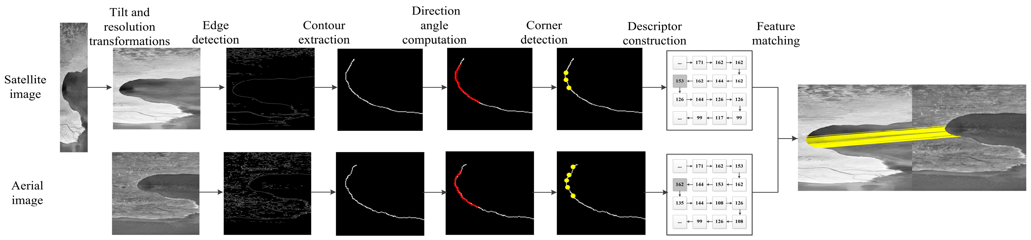
3. Materials and Methods

The proposed ECDAF algorithm is presented at a detailed level, and the schematic diagram is depicted in Figure 1. Firstly, according to the aerial camera attitude information provided by the POS system, the tilt and resolution transformations are performed on the orthorectified satellite image so that the aerial image and the satellite image have the same viewing angle and approximately equal pixel resolution. Then, an edge detection algorithm with an automatically set threshold is applied to extract the structural information of the scene. Next, the contour extraction algorithm is applied to extract the contour features of the aerial image and the satellite image, respectively, so that neighboring pixels in the edge image can be accessed one by one in an arranged order. Then, the pixels in the contour are divided into groups to form short curves, and the direction angle of each short curve is computed one by one. Next, corner points of each contour are detected according to the change of the direction angle of the short curve. Then, a feature descriptor with short curve direction angles is established centered on the corner point. Finally, the integrated matching similarity is computed to realize aerial–satellite image matching.

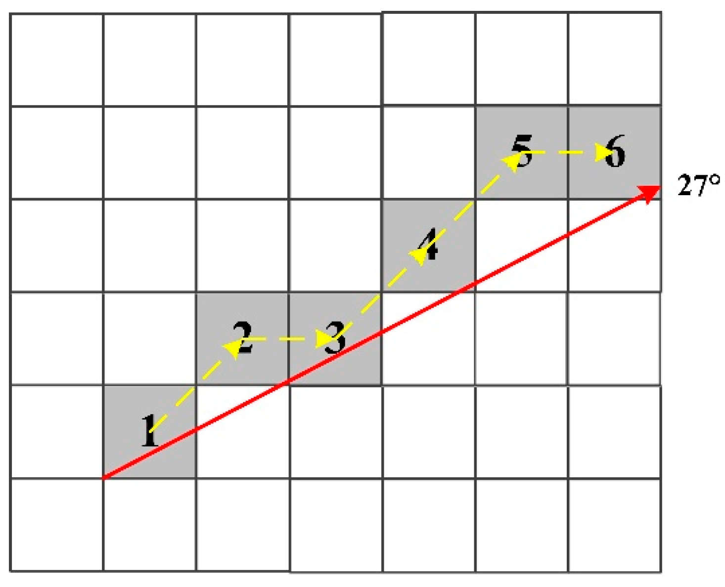
3.1. Curve Direction Angle

The direction angle between two pixels is defined based on the relative position of the eight neighboring pixels with respect to a given pixel, as shown in Figure 2. Define the $\overrightarrow{01}$ direction as $0^{\circ }$, the $\overrightarrow{02}$ direction as ${45}^{\circ }$, the $\overrightarrow{03}$ direction as ${90}^{\circ }$, the $\overrightarrow{04}$ direction as ${135}^{\circ }$, the $\overrightarrow{05}$ direction as ${180}^{\circ }$ or $-{180}^{\circ }$, the $\overrightarrow{06}$ direction as $-{135}^{\circ }$, the $\overrightarrow{07}$ direction as $-{90}^{\circ }$, and the $\overrightarrow{08}$ direction as $-{45}^{\circ }$. The specific angle value of the $\overrightarrow{05}$ direction is given by the definition below.

Define $\overrightarrow{02}$ direction and $\overrightarrow{08}$ direction, $\overrightarrow{03}$ direction and $\overrightarrow{07}$ direction, and $\overrightarrow{04}$ direction and $\overrightarrow{06}$ direction as opposite directions. Obviously, the sum of the angles of mutually opposite directions is equal to $0^{\circ }$.

A short curve consists of pixels adjacent to each other in the spatial domain, denoted as $C_s=\left\{p_1,p_2,\cdot \cdot \cdot ,p_{N_A}\right\}$. The specific angle value of the $\overrightarrow{05}$ direction is defined as follows:

$$\begin{array}{l}{\theta }_{\overrightarrow{05}}=\left\{\begin{array}{l}{180}^{\circ }, if p_{N_A}.y>p_1.y;\\ -{180}^{\circ }, if p_{N_A}.y<p_1.y,\end{array}\right.\\ \end{array}$$

(9)

where $p_1.y$ denotes the y-coordinate value of $p_1$ and $p_{N_A}.y$ denotes the y-coordinate value of $p_{N_A}$.

The $N_A$ pixels in a short curve form $(N_A-1)$ pixel direction angles, which is denoted in the order of arrangement as $\mathsf{\Phi }=\left\{{\theta }_1,{\theta }_2,\cdot \cdot \cdot ,{\theta }_{N_A-1}\right\}$. Assuming that $\mathsf{\Phi }$ contains $n_o$ pairs of opposite direction angles, the short curve direction angle is obtained by the following formula:

$$\alpha =\left\{\begin{array}{l}{0}^{\circ }, if p_{N_A}.y=p_1.y \& p_{N_A}.x\ge p_1.x;\\ -{180}^{\circ }, if p_{N_A}.y=p_1.y \& p_{N_A}.x<p_1.x;\\ {\displaystyle \sum _{i=1}^{N_A-1}{\theta }_i}/(N_A-1-2n_o), if p_{N_A}.y\ne p_1.y , \\ \end{array}\right.$$

(10)

where $p_1.x$ denotes the x-coordinate value of $p_1$ and $p_{N_A}.x$ denotes the x-coordinate value of $p_{N_A}$. The short curve direction angle $(N_A=6)$ is shown in Figure 3.

The contour of the scene is a long curve composed of pixels adjacent to each other in the spatial domain. A long curve is composed of N sections of sequentially connected short curves, forming short curve direction angles denoted as ${\Omega }_o=\left\{{\alpha }_1,{\alpha }_2,\cdot \cdot \cdot ,{\alpha }_N\right\}$. Short curve direction angles are used as features to construct a matching descriptor, which can realize aerial and satellite image matching.

3.2. Corner Point Detection

Pixels with large change in the short curve direction angles are defined as corners, and some of the corners are involved in image matching as feature points. In order to obtain more stable and reliable corners, a bilateral filter is applied to the short-curve direction angles in ${\mathsf{\Omega }}_o$, and the difference and distance of the direction angles are used as parameters. The bilateral filter removes the sudden change of the short curve direction angle in the local neighborhood and retains the change between short curve direction angles to the maximum extent. The formula of bilateral filter is defined as follows:

$${{\alpha }^{\prime }}_c={\displaystyle \frac{1}{k}}{\displaystyle \sum _{p\in \mathsf{\Gamma }}{g}_{{\sigma }_d}(p-c)g_{{\sigma }_a}(({\alpha }_p-{\alpha }_c)/m)}{\alpha }_p,$$

(11)

where k denotes the normalization coefficient, $p$ is the index of the short curve direction angle in the neighborhood, $c$ is the current index of the short curve direction angle, ${\alpha }_p$ denotes the degree of the short curve direction angle in the neighborhood, ${\alpha }_c$ denotes the degree of the current short curve direction angle, $m (m\ge 1)$ is the adjustment factor, and $g_{{\sigma }_d}(x)$ and $g_{{\sigma }_a}(x)$ denote the one-dimensional Gaussian function with standard deviation ${\sigma }_d$ and ${\sigma }_a$. The Gaussian function with standard deviation $\sigma$ is defined as follows:

$$g_{\sigma }(x)={\displaystyle \frac{1}{\sigma \sqrt{2\pi }}}{e}^{-{\displaystyle \frac{x^2}{2{\sigma }^2}}}.$$

(12)

The change in the degree of the short curve direction angle before and after filtering is shown in Figure 4.

The filtered short curve direction angles are represented as ${\mathsf{\Omega }}_f=\left\{{{\alpha }^{\prime }}_1,{{\alpha }^{\prime }}_2,\cdot \cdot \cdot ,{{\alpha }^{\prime }}_N\right\}$, and the elements in ${\mathsf{\Omega }}_f$ and ${\mathsf{\Omega }}_o$ correspond one to one. For each $i\in [1,N-1]$, if $\left|{{\alpha }^{\prime }}_{i+1}-{{\alpha }^{\prime }}_i\right|$ is greater than a threshold $K_d$, the corner is detected. The pixel $p_{N_A}$ at the end of the arrangement of $C_s=\left\{p_1,p_2,\cdot \cdot \cdot ,p_{N_A}\right\}$ involved in the computation of ${\alpha }_i$ is considered to be the corner.

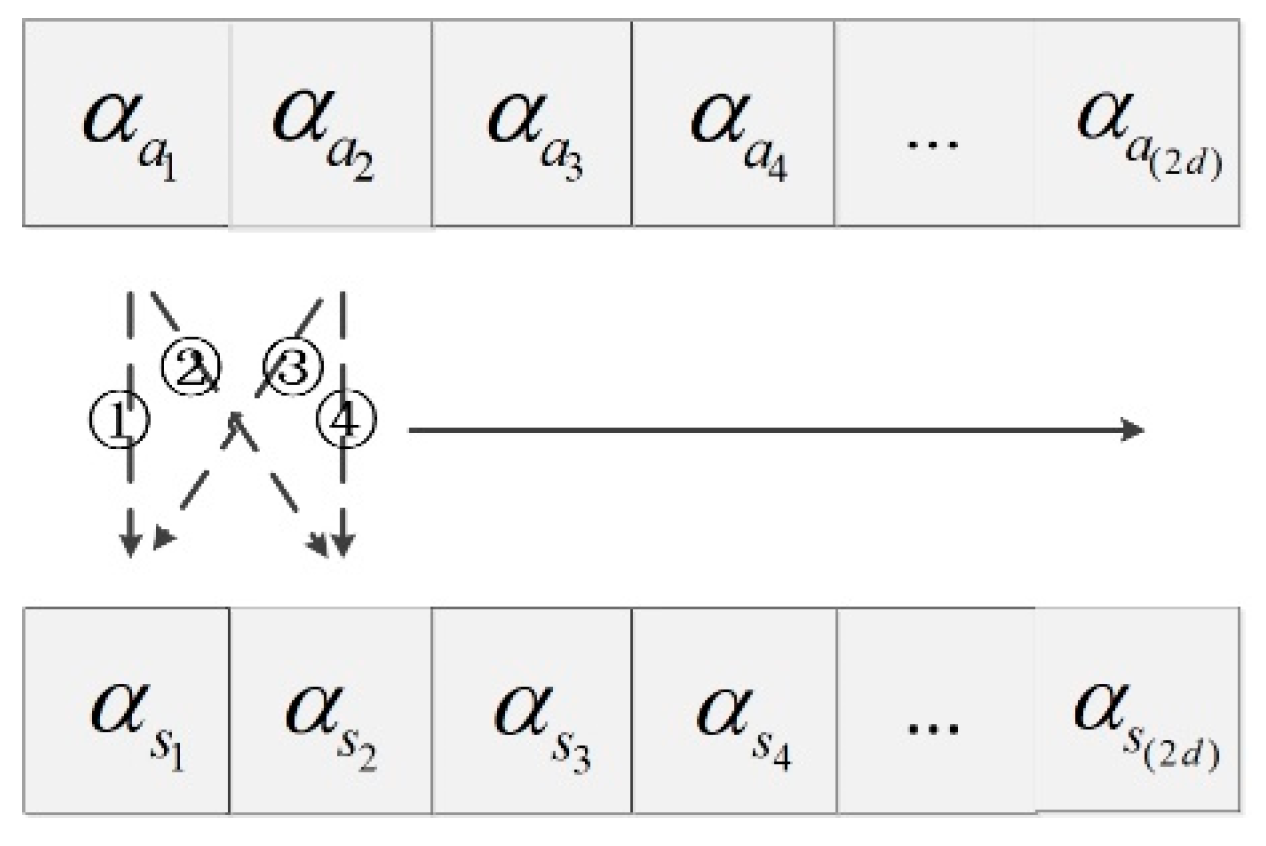
3.3. Descriptor Construction

The $d$ antecedent short curve direction angles arranged before the corner and the $d$ succeeding short curve direction angles arranged after the corner are connected as the feature descriptor, and the feature descriptor reflects the geometrical structure characteristics in the vicinity of the corner. The feature descriptor $FD$ is denoted as $FD=\left(P,N\right)$, $P$ denotes the antecedent short curve direction angle vector of the corner, and $N$ denotes the succeeding short curve direction angle vector of the corner.

The $l_2$-norm of the difference between $P$ and $N$ is computed. If ${‖P-N‖}_2$ is greater than a threshold $K_f$, the corresponding corner point is considered to be a feature point.

3.4. Feature Matching

The feature point description vector of the aerial image is denoted as $ADAV=\left[{\alpha }_{a_1} {\alpha }_{a_2} \cdot \cdot \cdot {\alpha }_{a_d} {\alpha }_{a_{(d+1)}} {\alpha }_{a_{(d+2)}}\cdot \cdot \cdot {\alpha }_{a_{(2d)}}\right]$ and the feature point description vector of the satellite image is denoted as $SDAV=\left[{\alpha }_{s_1} {\alpha }_{s_2} \cdot \cdot \cdot {\alpha }_{s_d} {\alpha }_{s_{(d+1)}} {\alpha }_{s_{(d+2)}}\cdot \cdot \cdot {\alpha }_{s_{(2d)}}\right]$. The comparison process between the description vectors is shown in Figure 5. We mark the index of the element in $ADAV$ as $i (1\le i\le 2d)$ and the index of the element in $SDAV$ as $j (1\le j\le 2d)$. We mark the vector storing the index of the matched aerial direction angles as $AIV$ and the vector storing the index of the matched satellite direction angles as $SIV$. We initialize $i$ and $j$ to 1, and complete a round of comparison in the order of step ① to step ④. If $\left|{\alpha }_{a_i}-{\alpha }_{s_j}\right|$ is smaller than a threshold $K_c$ in a certain step, we add $i$ to $AIV$ and $j$ to $SIV$, and then $i$ and $j$ are increased by 1 at the same time and enter the next round of comparison. Otherwise, $i$ and $j$ are increased by 1 and go directly to the next round of the comparison. The comparison terminates when $i$ or $j$ reaches $(2d+1)$.

After the above comparison process, the indexes of the matched direction angles are stored in $AIV$ and $SIV$ one by one.

The more the number of indexes stored in the vector, the higher the overall similarity of the curves. The similarity $s_n$ is computed with the following:

$$s_n=\left\{\begin{array}{l}{\displaystyle \frac{\log (N_v)}{A_n}}, if N_v\ge T_{on};\\ \\ -\infty , else,\end{array}\right.$$

(13)

where $N_v$ denotes the number of indexes contained in the vector, $A_n$ denotes the adjustment factor, and $T_{on}$ denotes the threshold.

The better the continuity of the indexes stored in the vector, the higher the local similarity of the curves. The similarity $s_c$ is computed with the following:

$$\begin{array}{l}{s}_c=\left\{\begin{array}{l}1-{\displaystyle \frac{{\displaystyle \sum _{i=1}^{N_v-1}((AIV[i+1]-AIV[i])+(SIV[i+1]-SIV[i]))}}{2\cdot A_c\cdot (N_v-1)}}, if {\mathsf{\Gamma }}_{oc}=true;\\ \\ -\infty , else,\end{array}\right.\\ \\ \\ {\mathsf{\Gamma }}_{oc}\equiv (AIV[i+1]-AIV[i])\le T_{oc } \&(SIV[i+1]-SIV[i])\le T_{oc}, for each i\in [1,N_v-1],\end{array}$$

(14)

where $N_v$ denotes the number of indexes contained in the vector, $A_c$ denotes the adjustment factor, and $T_{oc}$ denote the threshold.

The more concentrated the indexes near the corner, the more robust the matching result is. The similarity $s_f$ is computed with the following:

$$\begin{array}{l}{s}_f={\displaystyle \frac{{\displaystyle \sum _{i=1}^{N_v}(h(\left|AIV[i]-d\right|)+h(\left|SIV[i]-d\right|))}}{A_f}},\\ \\ h(x)=\left\{\begin{array}{l}(a-x^c)/b, if x\le T_{of};\\ \\ 0, else,\end{array}\right.\end{array}$$

(15)

where $N_v$ denotes the number of indexes contained in the vector, $A_f$ denotes the adjustment factor, $T_{of}$ denotes the threshold, $a$ is 16, $b$ is 16, and $c$ is 2.

The smaller the difference between the corresponding indexes stored in $AIV$ and $SIV$, the closer the shape of the curves. The similarity $s_b$ is computed with the following:

$$\begin{array}{l}{s}_b=\left\{\begin{array}{l}1-{\displaystyle \frac{{\displaystyle \sum _{i=1}^{N_v}(|AIV[i]-SIV[i]|)}}{A_b\cdot N_v}}, if {\mathsf{\Gamma }}_b=true;\\ \\ -\infty , else,\end{array}\right.\\ \\ {\mathsf{\Gamma }}_b\equiv if |AIV[i]-SIV[i]|\le T_{ob}, for each i\in [1,N_v],\end{array}$$

(16)

where $N_v$ denotes the number of indexes contained in the vector, $A_b$ denotes the adjustment factor, and $T_{ob}$ denotes the threshold.

The general similarity $s_g$ is computed with the following:

$$\begin{array}{l}{s}_g=s_n+s_c+s_f+s_b\\ \end{array}$$

(17)

If $s_g$ is greater than a threshold $T_g$, the matched points in aerial and satellite images are detected.

4. Results

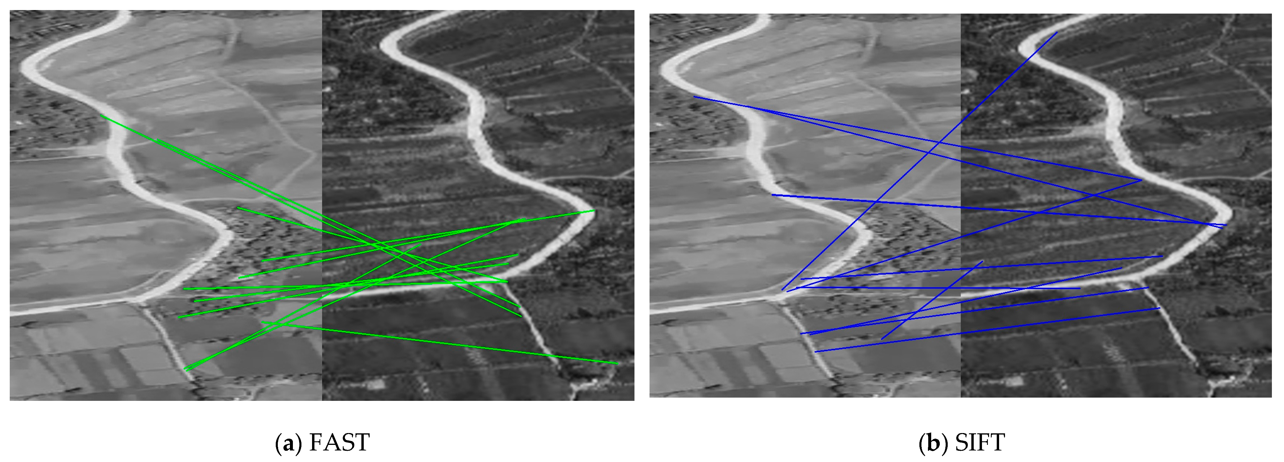
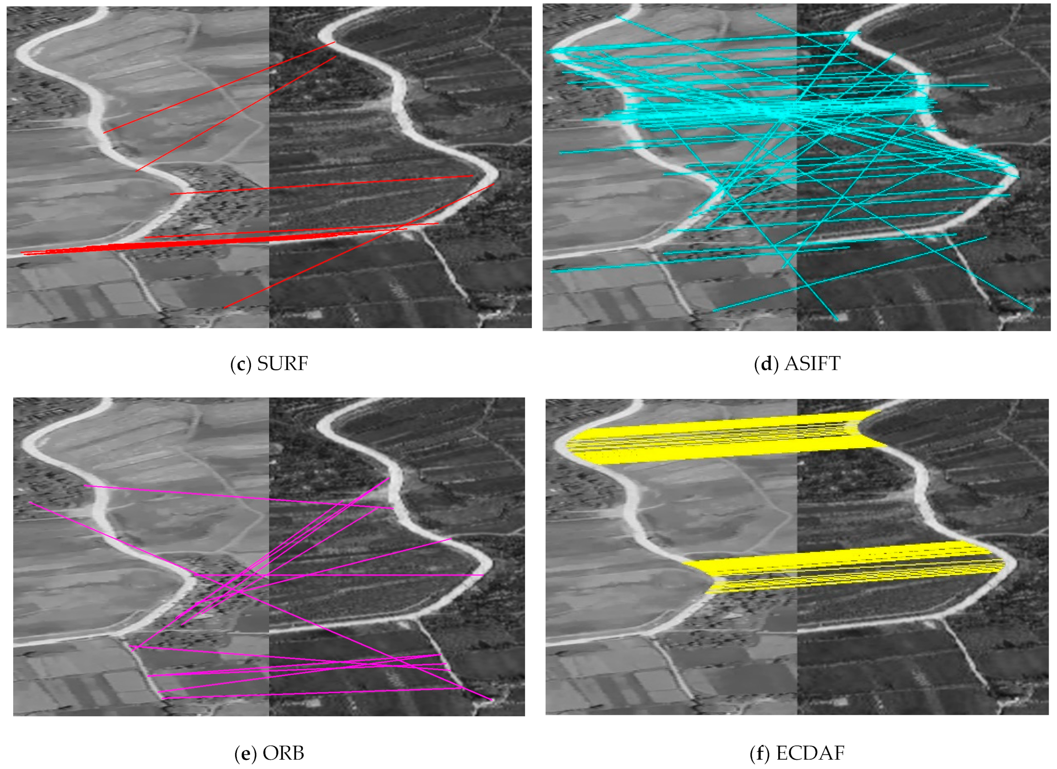
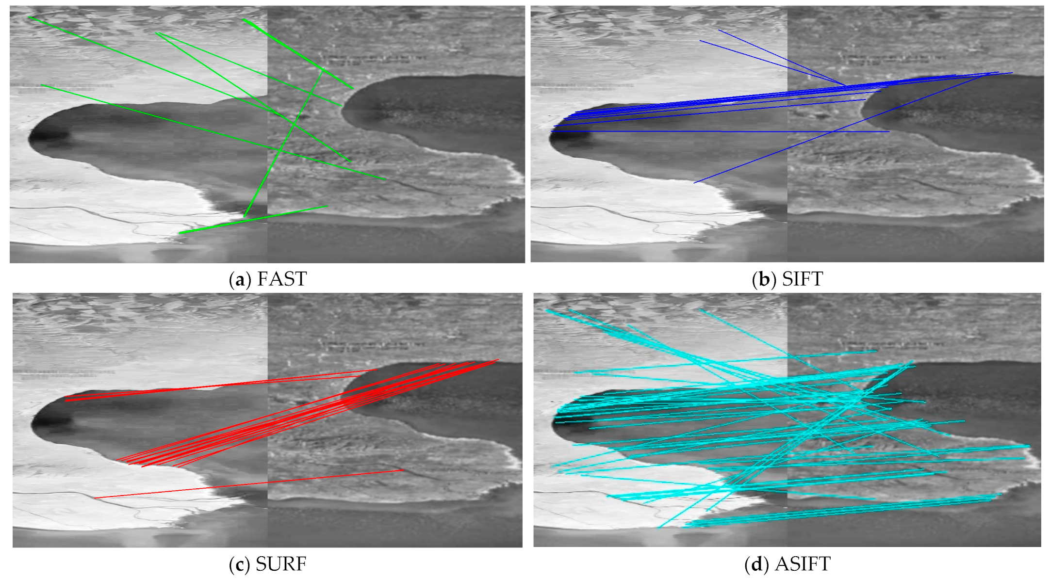
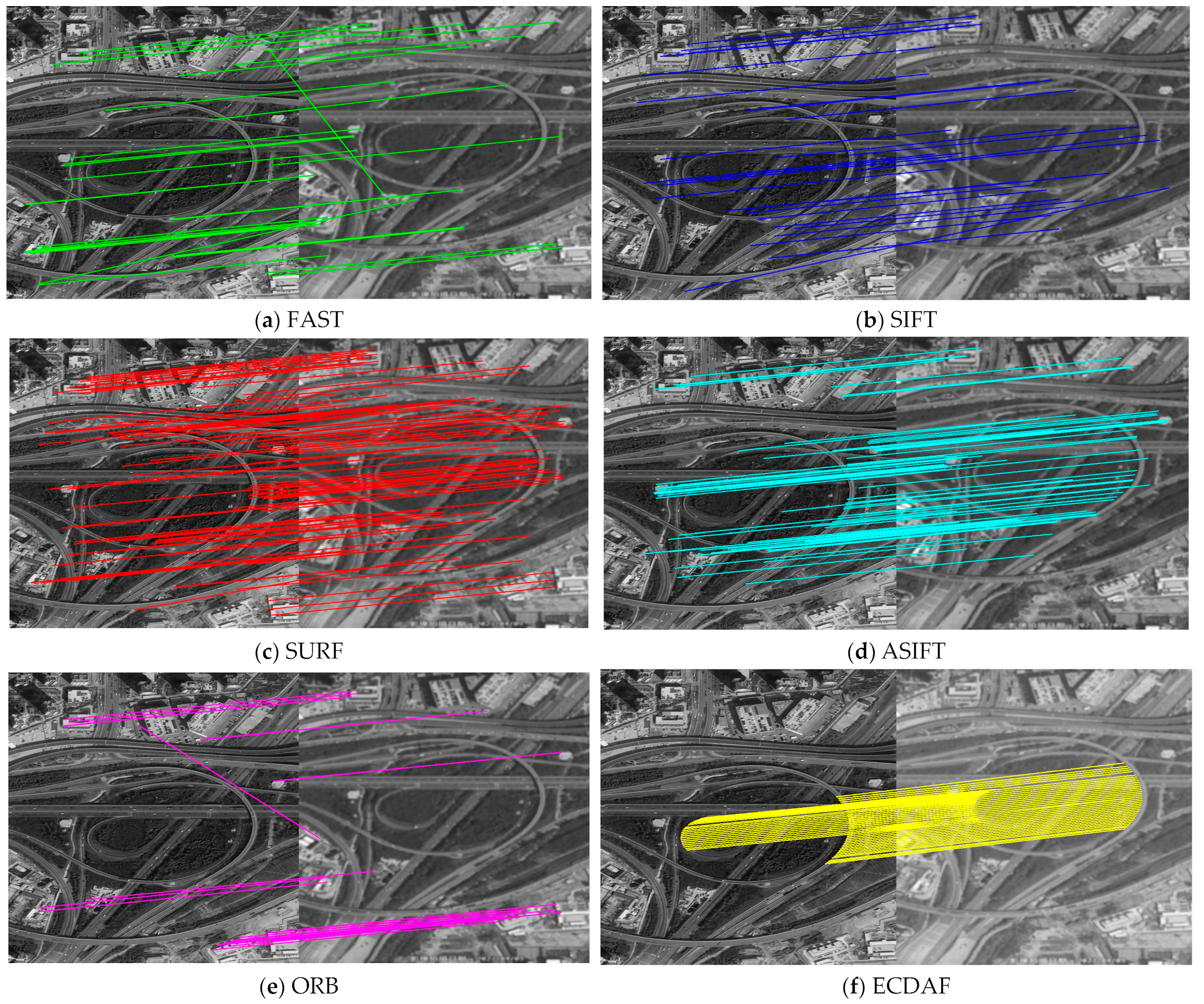
4.1. Qualitative Evaluation

Six groups of remote sensing images were applied in the experiments to test the proposed algorithm, with tilted satellite images on the left and inclined aerial images on the right. The six groups of images include forests, hills, farmland, lake, buildings, and flyover scenes, as shown in Figure 6, Figure 7, Figure 8, Figure 9, Figure 10 and Figure 11. Some features of the six groups of the inclined aerial images are recorded in

Table 1. Some features of six groups of the inclined aerial images.

Scene	Azimuth Angle	Pitch Angle	Flight Altitude	Imaging Distance
Forests	39.16°	71.38°	12.23 km	38.3 km
Hills	48.49°	56.31°	13.98 km	25.2 km
Farmland	68.62°	75.25°	8.15 km	32.0 km
Lake	79.84°	78.69°	8.57 km	43.7 km
Buildings	27.91°	65.93°	8.42 km	20.5 km
Flyover	43.38°	53.27°	8.93 km	14.9 km

.

For the forests scene, the contrast and SNR of aerial images are significantly lower than those of satellite images due to the large tilted imaging angle of aerial images and the influence of atmospheric absorption and scattering of light. The different sensors and imaging time lead to different distribution of gray values of the same region in aerial and satellite images. Traditional image matching algorithms, including FAST, SIFT, SURF, and ORB, are use local gray value distribution features to achieve image matching, and the matching performance of these algorithms is relatively poor. The ASIFT algorithm extracts the SIFT feature points in different viewpoints and then carries out feature point matching. The image perspective transformation avoids the effect of different local gray value distribution on image matching to a certain extent, and the matching effect of the ASIFT algorithm is still acceptable. The proposed algorithm performs image matching by extracting the edge features of the image, which is not affected by the change of the gray value distribution. It achieves a promising matching effect.

Due to the different imaging time for the hills scene, there are trees planted on the hills in the aerial image, while there are terraces planted on the hills in the satellite image. The matching effect of the FAST, SIFT, SURF, and ORB algorithms is poor, and the matching effect of the ASIFT algorithm is still acceptable. The structural features formed by the roads on the hills are relatively stable, and the proposed algorithm performs image matching by extracting the edge features of the roads on the hills. The matching effect of the proposed algorithm is promising, but due to the influence of the local shape change of the roads, the image matching effect is slightly reduced compared to the forests scene.

For the farmland scene, there are few changes in the gray value distribution of the same region in satellite images and aerial images, so the matching effect of the SIFT and SURF algorithms is improved. The effect of the FAST and ORB algorithms is still poor, and the matching effect of the ASIFT algorithm is still acceptable. The structural features of roads in farmland are stable, and the proposed algorithm is more effective.

For the lake scene, the imaging time and imaging sensors of the satellite image and aerial image are different, and the gray value distribution of the same region are different. Therefore, the matching effects of the FAST, SIFT, SURF, and ORB algorithms are unsatisfactory. The large difference in the distribution of gray values in the same region between the satellite image and the aerial image also leads to the matching effect of the ASIFT algorithm being obviously not as good as that of the previous three scenarios. The proposed algorithm extracts the stable edge features of the lake and then performs image matching, achieving a better matching effect.

For the buildings scene, the performance of the FAST and ORB algorithms is still poor. Due to the closer imaging distance and less variation in gray values, the SIFT, SURF, and ASIFT algorithms achieve encouraging matching results. The proposed algorithm utilizes the structural features of buildings to achieve image matching and obtains promising results.

For the flyover scene, due to the minimum pitch angle and the closest imaging distance, the features of the scene are relatively stable and all the matching algorithms achieve satisfactory results.

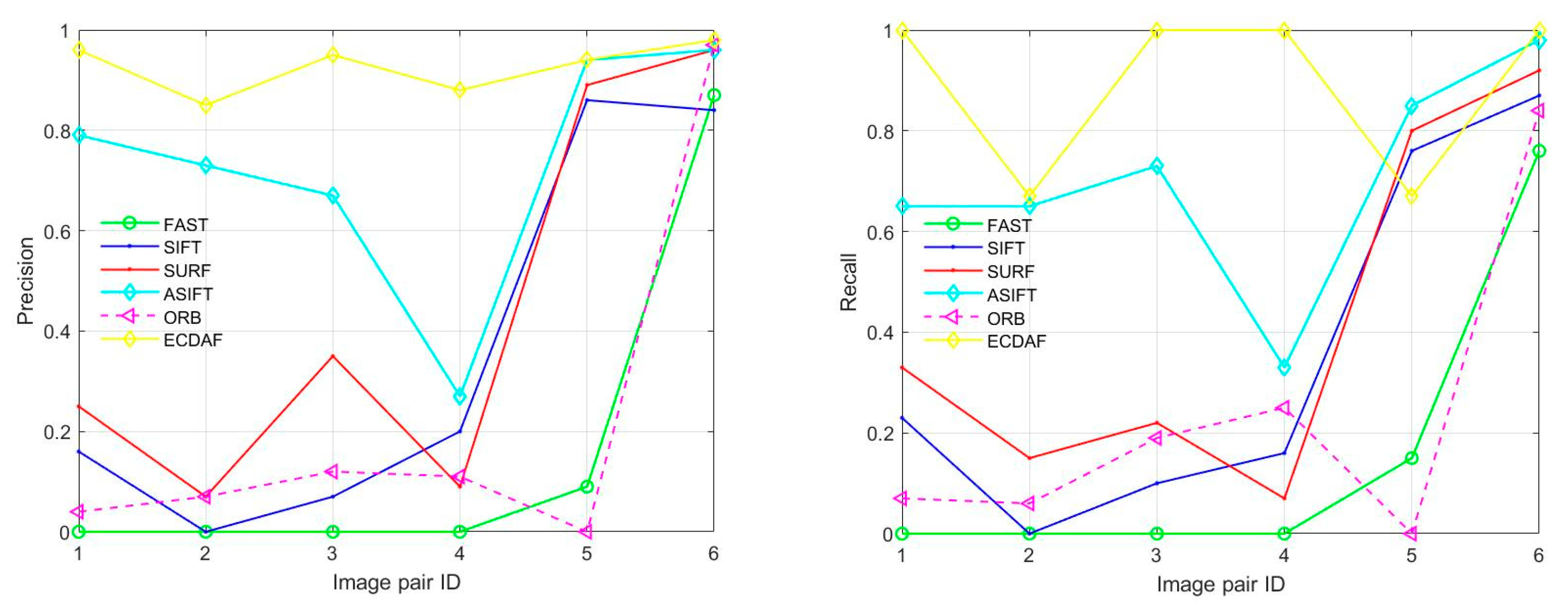
4.2. Precision and Recall

We used Precision and Recall measurements [42] to evaluate the performance of matching algorithms, as shown in Figure 12.

The proposed ECDAF algorithm achieved competitive matching results in terms of Precision and Recall, as shown in

Table 2. Precision and Recall (%) comparison. For each result in the bracket, the left is the precision and the right is the recall.

Scene	FAST	SIFT	SURF	ASIFT	ORB	ECDAF
Forests	(0.00, 0.00)	(16.7, 22.8)	(25.0, 32.8)	(79.1, 65.2)	(4.50, 7.22)	(96.0, 100)
Hills	(0.00, 0.00)	(0.00, 0.00)	(7.10, 15.3)	(73.2, 65.1)	(7.10, 5.92)	(85.0, 66.7)
Farmland	(0.00, 0.00)	(7.70, 10.4)	(35.0, 21.7)	(66.6, 72.9)	(12.5, 18.9)	(95.3, 100)
Lake	(0.00, 0.00)	(20.0, 15.8)	(9.10, 6.80)	(26.9, 32.6)	(11.1, 24.6)	(88.0, 100)
Buildings	(9.10, 15.3)	(85.7, 76.2)	(89.6, 80.3)	(93.9, 85.4)	(0.00, 0.00)	(93.7, 66.7)
Flyover	(87.5, 75.6)	(84.0, 86.9)	(96.5, 91.9)	(95.8, 97.8)	(96.9, 83.7)	(98.0, 100)

Bold numbers are used to highlight which result is the best among others in the row.

.

4.3. Running Time

The efficiency of the matching algorithms is contrasted on a computer with an Intel Core i7-1165G7 CPU and 16 GB DDR4 memory. All experiments are performed in Visual Studio 2022 software. Single-channel satellite images and aerial images with resolution of 822 × 822 are tested, and the running time in seconds of the matching algorithms is exhibited in

Table 3. Running time (seconds) of the matching algorithms over six scenarios.

Scene (ID)	FAST	SIFT	SURF	ASIFT	ORB	ECDAF
Forests (1)	2.83	9.11	2.71	98.85	0.69	12.37
Hills (2)	1.34	9.44	2.85	142.3	0.66	20.81
Farmland (3)	0.61	4.56	2.72	53.61	0.65	7.72
Lake (4)	0.64	3.99	1.67	22.19	0.62	4.19
Buildings (5)	1.63	6.41	2.54	88.24	0.68	10.15
Flyover (6)	3.22	8.36	3.19	103.8	0.83	18.92

.

The running time of the FAST, SURF, and ORB algorithms are all relatively short, and for the six scenes, the running time is less than 4 s. The running time of the SIFT algorithm is a little longer than that of the above three algorithms, and for the six scenes, the running time is less than 10 s. The running time of the proposed ECDAF algorithm is ranked second among all the six matching algorithms, and for the six scenes, the running times are 12.37 s, 20.81 s, 7.72 s, 4.19 s, 10.15 s, and 18.92 s, respectively. The texture of the lake scene is the simplest and the proposed algorithm extracts the fewest edges, resulting in the shortest running time of the six scenarios. The ASIFT algorithm has the longest running time for the six scenes, and the running time is significantly longer than the other five matching algorithms. The running time statistics of the matching algorithms are shown in Figure 13.

4.4. Parameter Setting

The number of pixels contained in each short curve segment $N_A$, if set too large, will result in the omission of corner points, and vice versa, will result in the false detection of corner points. We set the value of $N_A$ to 6. The number of direction angles of the antecedent or successor short curves in the corner descriptor $d$, if set too large, will cause the algorithm to take too long to run, and vice versa, it will cause false matching. The value of $d$ is set to 20. The threshold for detecting the difference between the antecedent and the successor short curve direction angles $K_f$, if set too large, will cause missed detection of the feature points, and vice versa, will cause the false detection of the feature points. The value of $K_f$ is set to 40. The comparison threshold of the short curve direction angles $K_c$, if set too large, will cause false matches, and vice versa, will cause the omission of matched feature points. The value of $K_c$ is set to 10. Other parameters setting are shown in

Table 4. Parameters setting table.

Number	Parameter	Value	Number	Parameter	Value
1	$K_d$	35	5	$A_f$	12.4
2	$A_n$	4.1	6	$T_{of}$	3
3	$T_{on}$	28	7	$A_b$	6.6
4	$A_c$	8	8	$T_{ob}$	3

.

5. Discussion

In this paper, an inclined aerial image and satellite image matching algorithm based on edge curve direction angle features is proposed. The proposed algorithm extracts the structural information of the remote sensing image and overcomes the effects of the low contrast and low SNR of aerial images, as well as the differences in the gray value of aerial image and satellite image of the same region. The proposed ECDAF algorithm offers promising outcomes for remote sensing images of forests, hills, farmland, and lake scenes, as shown in Figure 6, Figure 7, Figure 8 and Figure 9. Compared with other state-of-the-art image matching algorithms, the proposed algorithm has the highest matching accuracy, as shown in Figure 10. In conclusion, the proposed algorithm achieves promising effect for large inclination angle and long distance aerial image and satellite image matching.

The proposed algorithm has the disadvantage of long running time, and the part of the algorithm comparing the degree of the direction angle and the part of matching similarity computation consumes significant running time. In future research work, we will further optimize the matching algorithm for the above two parts to improve the running speed of the algorithm while ensuring high matching accuracy.

6. Conclusions

A set of algorithms for matching inclined aerial image and satellite image is designed, including tilt and resolution transformations, edge detection, contour extraction, curve direction angle computation, corner point detection, descriptor construction, and feature matching.

We firstly proposed the concept of curve direction angle, and then defined the direction angle between two pixels and the short curve direction angle formed by a number of pixels. Then, we realized a matching similarity computation method that incorporates multiple factors to achieve robust remote sensing image matching using the structural features of the scenery. The proposed algorithm is able to overcome the effect on image matching caused by the low contrast and low SNR of aerial images, as well as the difference in gray values between aerial image and satellite image of the same region. Experiments on a variety of remote sensing scenes confirm that the ECDAF algorithm is quite competitive in terms of matching accuracy and algorithm stability. Future research will focus on refining the proposed algorithm to shorten the running time while maintaining high matching performance.

References

1. Yang, H.; Huang, C.; Wang, F.; Song, K.; Yin, Z. Robust semantic template matching using a superpixel region binary descriptor. IEEE Trans. Image Process. 2019, 28, 3061–3074. [Google Scholar] [CrossRef] [PubMed]
2. Zhao, C.; Cao, Z.; Yang, J.; Xian, K.; Li, X. Image feature correspondence selection: A comparative study and a new contribution. IEEE Trans. Image Process. 2020, 29, 3506–3519. [Google Scholar] [CrossRef] [PubMed]
3. Sun, J.; Shen, Z.; Wang, Y.; Bao, H.; Zhou, X. LoFTR: Detector free local feature matching with transformers. In Proceedings of the 2021 IEEE/CVF Conference on Computer Vision and Pattern Recognition (CVPR), Nashville, TN, USA, 10–25 June 2021; pp. 8918–8927. [Google Scholar]
4. Zhang, H.; Lei, L.; Ni, W.; Cheng, K.; Tang, T.; Wang, P.; Kuang, G. Registration of Large Optical and SAR Images with Non-Flat Terrain by Investigating Reliable Sparse Correspondences. Remote Sens. 2023, 15, 4458. [Google Scholar] [CrossRef]
5. Ma, J.; Jiang, J.; Zhou, H.; Zhao, J.; Guo, X. Guided locality preserving feature matching for remote sensing image registration. IEEE Trans. Geosci. Remote Sens. 2018, 56, 4435–4447. [Google Scholar] [CrossRef]
6. Feng, R.; Shen, H.; Bai, J.; Li, X. Advances and opportunities in remote sensing image geometric registration: A systematic review of state-of-the-art approaches and future research directions. IEEE Geosci. Remote Sens. Mag. 2021, 9, 120–142. [Google Scholar] [CrossRef]
7. Ma, J.; Zhao, J.; Tian, J.; Yuille, A.; Tu, Z. Robust point matching via vector field consensus. IEEE Trans. Image Process. 2014, 23, 1706–1721. [Google Scholar] [CrossRef]
8. He, J.; Jiang, X.; Hao, Z.; Zhu, M.; Gao, W.; Liu, S. LPHOG: A Line Feature and Point Feature Combined Rotation Invariant Method for Heterologous Image Registration. Remote Sens. 2023, 15, 4548. [Google Scholar] [CrossRef]
9. Sommervold, O.; Gazzea, M.; Arghandeh, R. A Survey on SAR and Optical Satellite Image Registration. Remote Sens. 2023, 15, 850. [Google Scholar] [CrossRef]
10. Bellavia, F. SIFT matching by context exposed. IEEE Trans. Pattern Anal. Mach. Intell. 2023, 45, 2445–2457. [Google Scholar] [CrossRef]
11. Zhang, X.; Zhou, Y.; Qiao, P.; Lv, X.; Li, J.; Du, T.; Cai, Y. Image Registration Algorithm for Remote Sensing Images Based on Pixel Location Information. Remote Sens. 2023, 15, 436. [Google Scholar] [CrossRef]
12. Lowe, D. Distinctive image features from scale-invariant keypoints. Int. J. Comput. Vis. 2004, 60, 91–110. [Google Scholar] [CrossRef]
13. Pang, S.; Ge, J.; Hu, L.; Guo, K.; Zheng, Y.; Zheng, C.; Zhang, W.; Liang, J. RTV-SIFT: Harnessing Structure Information for Robust Optical and SAR Image Registration. Remote Sens. 2023, 15, 4476. [Google Scholar] [CrossRef]
14. Bay, H.; Tuytelaars, T.; Gool, L. Surf: Speeded up robust features. In Proceedings of the Computer Vision—ECCV 2006, Graz, Austria, 7–13 May 2006; pp. 404–417. [Google Scholar]
15. Yao, G.; Cui, J.; Deng, K.; Zhang, L. Robust harris corner matching based on the quasi-homography transform and self-adaptive window for wide-baseline stereo images. IEEE Trans. Geosci. Remote Sens. 2018, 56, 559–574. [Google Scholar] [CrossRef]
16. Rosten, E.; Drummond, T. Machine learning for high-speed corner detection. In Proceedings of the Computer Vision—ECCV 2006, Graz, Austria, 7–13 May 2006; pp. 430–443. [Google Scholar]
17. Michael, C.; Vincent, L.; Christoph, S.; Pascal, F. BRIEF: Binary robust independent elementary features. In Proceedings of the Computer Vision—ECCV 2010, Heraklion, Greece, 5–11 September 2010; pp. 778–792. [Google Scholar]
18. Ethan, R.; Vincent, R.; Kurt, K.; Gary, B. ORB: An efficient alternative to SIFT or SURF. In Proceedings of the 2011 IEEE International Conference on Computer Vision (ICCV), Barcelona, Spain, 6–13 November 2011; pp. 2564–2571. [Google Scholar]
19. Yu, G.; Morel, J. ASIFT: An algorithm for fully affine invariant comparison. Image Process. 2011, 1, 11–38. [Google Scholar] [CrossRef]
20. Wang, Z.; Wu, F.; Hu, Z. MSLD: A robust descriptor for line matching. Pattern Recognit. 2009, 42, 941–953. [Google Scholar] [CrossRef]
21. Zhang, L.; Koch, R. An efficient and robust line segment matching approach based on LBD descriptor and pairwise geometric consistency. J. Vis. Commun. Image Represent. 2013, 24, 794–805. [Google Scholar] [CrossRef]
22. Wang, L.; Neumann, U.; You, S. Wide-baseline image matching using line signatures. In Proceedings of the 2009 IEEE International Conference on Computer Vision (ICCV), Kyoto, Japan, 29 September–2 October 2009; pp. 1311–1318. [Google Scholar]
23. López, J.; Santos, R.; Fdez-Vidal, X.; Pardo, X. Two-view line matching algorithm based on context and appearance in low-textured images. Pattern Recognit. 2015, 48, 2164–2184. [Google Scholar] [CrossRef]
24. Lourakis, M.; Halkidis, S.; Orphanoudakis, S. Matching disparate views of planar surfaces using projective invariants. Image Vis. Comput. 2000, 18, 673–683. [Google Scholar] [CrossRef]
25. Fan, B.; Wu, F.; Hu, Z. Robust line matching through line-point invariants. Pattern Recognit. 2012, 45, 794–805. [Google Scholar] [CrossRef]
26. Zhu, H.; Jiao, L.; Ma, W.; Liu, F.; Zhao, W. A novel neural network for remote sensing image matching. IEEE Trans. Neural Netw. Learn. Syst. 2019, 30, 2853–2865. [Google Scholar] [CrossRef]
27. Han, X.; Leung, T.; Jia, Y.; Sukthankar, R.; Berg, A. MatchNet: Unifying feature and metric learning for patch-based matching. In Proceedings of the 2015 IEEE Conference on Computer Vision and Pattern Recognition (CVPR), Boston, MA, USA, 7–12 June 2015; pp. 3279–3286. [Google Scholar]
28. Quan, D.; Liang, X.; Wang, S.; Wei, S.; Li, Y.; Huyan, N.; Jiao, L. AFD-Net: Aggregated feature difference learning for cross-spectral image patch matching. In Proceedings of the 2019 IEEE/CVF International Conference on Computer Vision (ICCV), Seoul, Republic of Korea, 27 October–2 November 2019; pp. 3017–3026. [Google Scholar]
29. Dusmanu, M.; Rocco, I.; Pajdla, T.; Pollefeys, M.; Sivic, J.; Torii, A.; Sattler, T. D2-Net: A trainable CNN for joint description and detection of local features. In Proceedings of the 2019 IEEE/CVF Conference on Computer Vision and Pattern Recognition (CVPR), Long Beach, CA, USA, 15–20 June 2019; pp. 8084–8093. [Google Scholar]
30. Ma, W.; Zhang, J.; Wu, Y.; Jiao, L.; Zhu, H.; Zhao, W. A novel two-step registration method for remote sensing images based on deep and local features. IEEE Trans. Geosci. Remote Sens. 2019, 57, 4834–4843. [Google Scholar] [CrossRef]
31. Zhang, H.; Ni, W.; Yan, W.; Xiang, D.; Wu, J.; Yang, X.; Bian, H. Registration of multimodal remote sensing image based on deep fully convolutional neural network. IEEE J. Sel. Top. Appl. Earth Obs. Remote Sens. 2019, 12, 3028–3042. [Google Scholar] [CrossRef]
32. Li, Z.; Zhang, H.; Huang, Y. A Rotation-Invariant Optical and SAR Image Registration Algorithm Based on Deep and Gaussian Features. Remote Sens. 2021, 13, 2628. [Google Scholar] [CrossRef]
33. Uss, M.; Vozel, B.; Lukin, V.; Chehdi, K. Exhaustive search of correspondences between multimodal remote sensing images using convolutional neural network. Sensors 2022, 22, 1231–1247. [Google Scholar] [CrossRef]
34. Ma, J.; Jiang, X.; Jiang, J.; Zhao, J.; Guo, X. LMR: Learning a two-class classifier for mismatch removal. IEEE Trans. Image Process. 2019, 28, 4045–4059. [Google Scholar] [CrossRef]
35. Quan, D.; Wei, H.; Wang, S.; Gu, Y.; Hou, B.; Jiao, L. A novel coarse-to-fine deep learning registration framework for multimodal remote sensing images. IEEE Trans. Geosci. Remote Sens. 2023, 61, 5108316. [Google Scholar] [CrossRef]
36. Yao, Y.; Zhang, Y.; Wan, Y.; Liu, X.; Yan, X.; Li, J. Multi-modal remote sensing image matching considering co-occurrence filter. IEEE Trans. Image Process. 2022, 31, 2584–2597. [Google Scholar] [CrossRef]
37. Richard, H.; Andrew, Z. Multiple View Geometry in Computer Vision, 2nd ed.; Cambridge University Press: Cambridge, UK, 2004; pp. 36–58. [Google Scholar]
38. Canny, J. A computational approach to edge detection. IEEE Trans. Pattern Anal. Mach. Intell. 1986, 8, 679–698. [Google Scholar] [CrossRef]
39. Bao, P.; Zhang, L.; Wu, X. Canny edge detection enhancement by scale multiplication. IEEE Trans. Pattern Anal. Mach. Intell. 2005, 27, 1485–1490. [Google Scholar] [CrossRef]
40. Xu, Q.; Varadarajan, S.; Chakrabarti, C.; Karam, L. A distributed canny edge detector: Algorithm and FPGA implementation. IEEE Trans. Image Process. 2014, 23, 2944–2960. [Google Scholar] [CrossRef]
41. Suzuki, S.; Abe, K. Topological structural analysis of digitized binary images by border following. Comput. Vis. Graph. Image Process. 1985, 30, 32–46. [Google Scholar] [CrossRef]
42. Bian, J.; Lin, W.; Liu, Y.; Zhang, L.; Yeung, S.; Cheng, M.; Reid, I. GMS: Grid–based motion statistics for fast, ultra–robust feature correspondence. In Proceedings of the 2017 IEEE/CVF Conference on Computer Vision and Pattern Recognition (CVPR), Honolulu, HI, USA, 21–26 July 2017; pp. 5183–5192. [Google Scholar]
Figure 1. Schematic of the proposed method with edge curve direction angle features algorithm.
Remotesensing 17 00268 g001
Figure 2. Schematic diagram of direction angle between two pixels.
Remotesensing 17 00268 g002
Figure 3. Schematic diagram of short curve direction angle. The yellow arrow represents the direction angle between two pixels and the red arrow represents the short curve direction angle.
Remotesensing 17 00268 g003
Figure 4. Diagram of the change in the degree of the short curve direction angles before and after filtering.
Remotesensing 17 00268 g004
Figure 5. Diagram of description vectors comparison.
Remotesensing 17 00268 g005
Figure 6. Comparison of forests scene matching results.
Remotesensing 17 00268 g006
Figure 7. Comparison of hills scene matching results.
Remotesensing 17 00268 g007aRemotesensing 17 00268 g007b
Figure 8. Comparison of farmland scene matching results.
Remotesensing 17 00268 g008aRemotesensing 17 00268 g008b
Figure 9. Comparison of lake scene matching results.
Remotesensing 17 00268 g009aRemotesensing 17 00268 g009b
Figure 10. Comparison of buildings scene matching results.
Remotesensing 17 00268 g010
Figure 11. Comparison of flyover scene matching results.
Remotesensing 17 00268 g011
Figure 12. Statistics of the precision and recall over six scenarios.
Remotesensing 17 00268 g012
Figure 13. Statistics of the running time on each scenario.
Remotesensing 17 00268 g013