An Effective Robust Total Least-Squares Solution Based on “Total Residuals” for Seafloor Geodetic Control Point Positioning

Abstract

Global Navigation Satellite System/Acoustic (GNSS/A) underwater positioning technology is attracting more and more attention as an important technology for building the marine Positioning, Navigation, and Timing (PNT) system. The random error of the tracking point coordinate is also an important error source that affects the accuracy of GNSS/A underwater positioning. When considering its effect on the mathematical model of GNSS/A underwater positioning, the Total Least-Squares (TLS) estimator can be used to obtain the optimal position estimate of the seafloor transponder, with weak consistency and asymptotic unbiasedness. However, the tracking point coordinates and acoustic ranging observations are inevitably contaminated by outliers because of human mistakes, failure of malfunctioning instruments, and unfavorable environmental conditions. A robust alternative needs to be introduced to suppress the adverse effect of outliers. The conventional Robust TLS (RTLS) strategy is to adopt the selection weight iteration method based on each single prediction residual. Please note that the validity of robust estimation depends on a good agreement between residuals and true errors. Unlike the Least-Squares (LS) estimation, the TLS estimation is unsuitable for residual prediction. In this contribution, we propose an effective RTLS_Eqn estimator based on “total residuals” or “equation residuals” for GNSS/A underwater positioning. This proposed robust alternative holds its robustness in both observation and structure spaces. To evaluate the statistical performance of the proposed RTLS estimator for GNSS/A underwater positioning, Monte Carlo simulation experiments are performed with different depth and error configurations under the emulational marine environment. Several statistical indicators and the average iteration time are calculated for data analysis. The experimental results show that the Root Mean Square Error (RMSE) values of the RTLS_Eqn estimator are averagely improved by 12.22% and 10.27%, compared to the existing RTLS estimation method in a shallow sea of 150 m and a deep sea of 3000 m for abnormal error situations, respectively. The proposed RTLS estimator is superior to the existing RTLS estimation method for GNSS/A underwater positioning.

1. Introduction

The marine Positioning, Navigation, and Timing (PNT) system is an important infrastructure for the exploration, development, and utilization of marine resources, which is a natural continuation of the comprehensive PNT system in the ocean [1]. The seafloor geodetic control network is a key component of the marine PNT system, and it will promote the establishment of an International Terrestrial Reference Frame (ITRF) that can seamlessly connect the land and the ocean [2,3,4]. In recent decades, Global Navigation Satellite System/Acoustic (GNSS/A) underwater positioning technology has been studied systematically and then used to establish the seafloor geodetic control network in support of various engineering and science activities, including underwater navigation, seafloor geodetic deformation measurement, marine environment protection, and marine construction [5,6,7,8,9,10,11,12,13,14,15,16,17]. The idea of GNSS/A underwater positioning technology was first proposed by the Scripps Institute of Oceanography (SIO) [5,18]. Its purpose is to accurately acquire the position of the seafloor transponder through the relay of a sea-surface dynamic or static measurement platform. The GNSS/A underwater positioning system is composed of two parts. The surface part is to monitor the transducer’s positions by satellite-based difference positioning, Precise Point Positioning (PPP), Real-Time Kinematic (RTK) positioning or post-processing differential positioning, and other positioning methods [19,20]. The underwater part is to estimate the seafloor transponder’s position according to the acoustic ranging observations [21].

Different scholars and engineers have conducted extensive, thorough research on GNSS/A underwater positioning technology from several aspects, such as tracking line design, the systematic error handling strategy, the mathematical model, the parameter estimation method, and so on. Many researchers suggest that a symmetrical sea-surface GNSS/A tracking line in the three-dimensional space helps eliminate the systematic errors of spatial symmetric distribution [14,22,23]. The surveying vessel sails almost on a plane to conduct underwater acoustic ranging, which increases the risk of rank deficit during data processing and then biases the final vertical positioning result. A cross-configuration tracking line can be employed to improve the bias identification ability in the vertical direction [14,16,24]. Another effective way to improve vertical positioning accuracy is to apply the depth constraints offered by pressure gauges [25,26]. The reliability of underwater acoustic ranging is a prerequisite for high-accuracy GNSS/A positioning. The acoustic ranging error, including the acoustic ray bending error related to range bias and the acoustic speed variation error related to time bias, is the main systematic error source of the GNSS/A underwater positioning system [16]. Two main strategies can be used to deal with this kind of systematic error. One is to parameterize the acoustic ranging errors and then introduce them into the functional model with the accurate acoustic speed field information [7,11,27]. Another is to weaken the adverse effect of acoustic ranging errors by utilizing underwater differential positioning techniques, including single difference and double difference [23,24,28]. Recently, the resilient functional model has also been proposed to compensate for systematic errors [16]. Although several research results have been obtained from the data processing of acoustic ranging errors, no method is superior to other methods. The acoustic ranging error is still the most important factor in restricting the accuracy of GNSS/A underwater positioning. A proper mathematical model, including the functional model and the stochastic model, is necessary to achieve the high-accuracy GNSS/A underwater positioning [5,15,22]. The functional model is to establish the geometric or physical relationship between the acoustic ranging observations and the unknown seafloor transponder’s position [29]. The acoustic observation equation is the most widely used functional model for the GNSS/A underwater positioning system. It is even possible to introduce the GNSS observation equation to compose a more complex and comprehensive functional model. The stochastic model is to show the statistical property of random quantities, and it is usually achieved by a predefined variance–covariance matrix [30,31]. Any misspecification of the stochastic model could have disastrous consequences for the GNSS/A underwater data processing. In the last few years, many stochastic models have been defined based on actual requirements for the GNSS/A underwater data processing, such as the equal-weighted stochastic model, the ray incidence angle stochastic model [21,32], the real-time stochastic model [33], the signal intensity transmission loss stochastic model, etc. [34]. These methods can improve the estimation accuracy of the seafloor transponder’s position to different degrees. The choice of parameter estimation methods is closely related to the mathematical model used during the GNSS/A underwater data processing [31]. The processing strategy of random errors is an important basis for selecting parameter estimation methods [35]. If the tracking point coordinates are treated as known quantities, the Gauss–Markov (GM) model can be used to establish the acoustic observation equation. Then, the classical LS estimator is suitable to deal with the GNSS/A underwater positioning [5,18,36]. The tracking point coordinates, obtained by GNSS technology, are also affected by random errors. By applying the error propagation law, an Extended Least-Squares (ELS) estimator is proposed for obtaining a more accurate seafloor transponder’s position [28]. Please note that only the effect of random errors from the tracking point coordinates on the stochastic model is considered during adoption of the ELS estimator. If one considers the effect of random errors from the tracking point coordinates on both the functional and stochastic models, the Errors-In-Variables (EIV) model is better suited for establishing acoustic observation equations, and the Total Least-Squares (TLS) estimator can obtain the optimal position estimate of the seafloor transponder with weak consistency and asymptotic unbiasedness [35,37,38,39,40,41,42,43,44,45].

There is always a possibility that direct or indirect measurements are also contaminated by outliers because of human mistakes, failure of malfunctioning instruments, and unfavorable environmental conditions [46]. Even today, when Artificial Intelligence Technology (AIT) is widely used, one still cannot reduce the probability of outlier occurrence. The unknown seafloor transponder’s position can be estimated by the Robust Least-Squares (RLS) estimator to suppress the adverse effect of outliers [47,48]. Considering that the tracking point coordinates also contain random errors, the EIV model is a more complete mathematical model, and the Robust TLS (RTLS) estimator has also been applied to the data processing of GNSS/A underwater positioning [49,50,51]. Both robust estimators mentioned above are designed based on M-estimation and realized by the selection weight iteration method. Please note that the validity of M-estimation depends on a good agreement between residuals and true errors. Van Huffel and Vandewalle (1991) have clarified that the TLS estimator is not suitable for residual prediction [35]. Therefore, the present RTLS estimation algorithms based on single-predicted residuals do have some defects. In this contribution, we use the “total residuals” or “equation residuals” instead of single residuals for re-weighting to design the corresponding RTLS estimation algorithm, which is called RTLS_Eqn [38,42]. The standardized residuals and the robust unit weight variance factor are also utilized to ensure its robustness in both observation and structure spaces. Then, the proposed RTLS estimation algorithm is adopted to estimate the seafloor transponder’s position, and compared to other related algorithms to illustrate its robustness and effectiveness.

As described above, we briefly reviewed the key technologies of the GNSS/A underwater positioning system. In the following section, the nonlinear acoustic observation equation will be established based on the EIV model; the TLS solution is deduced in detail; and then the “total residuals” are thoroughly analyzed and deconstructed. A novel RTLS estimation algorithm is designed for GNSS/A underwater positioning. Finally, Monte Carlo simulation experiments are conducted to illustrate the robustness and effectiveness of the proposed method, and the conclusions and perspectives are summarized.

2. Materials and Methods

2.1. Total Least-Squares Estimator for Seafloor Geodetic Control Point Positioning

GNSS/A underwater positioning can be achieved by a surveying vessel sailing above a seafloor transponder along a planning tracking line, as shown in Figure 1. The acoustic ranging is periodically carried out between a transducer installed on the bottom of a surveying vessel and the transponder embedded on the seafloor. The position of the surveying vessel can be obtained by the real-time or post-processing positioning of a GNSS receiver installed on the deck at each observation of acoustic ranging. The relative position between the GNSS antenna and the transducer in the Vessel Coordinate System (VCS) can be determined by the high-accuracy measurement in advance. In the course of acoustic ranging, high-accuracy attitude measurements are also conducted to compensate for the surveying vessel’s attitude by an attitude sensor. Combining the above information, the 3D coordinate of the seafloor geodetic control point can be expected to be obtained with high accuracy [5,16,28].

As shown in Figure 1, the position of the seafloor transponder can be achieved by space resection. The general acoustic observation equation reads

$$l_i=f_i\left(x_i,x\right)+\delta l_{di}+\delta l_{vi}+e_{li}$$

(1)

where $x_i=\left(\begin{array}{ccc}{n}_i& e_i& u_i\end{array}\right)$ stands for the transducer’s position at an observation epoch $T_i(i=1,\dots ,m)$, which is also the so-called position of the surveying vessel obtained using GNSS technology; $x=\left(\begin{array}{ccc}n& e& u\end{array}\right)$ stands for the position of the seafloor transponder; $f_i\left(x_i,x\right)=\sqrt{{\left(n_i-n\right)}^2+{\left(e_i-e\right)}^2+{\left(u_i-u\right)}^2}$ stands for the geometric distance between $x_i$ and $x$; $l_i$ stands for a single-trip range from $x_i$ to $x$ at epoch $T_i$, and $e_{li}$ denotes the corresponding random error of $l_i$; $\delta l_{di}$ stands for the systemic error related to the transponder hardware delay, which can be ignored during data processing because it has been controlled in the order of millimeters; and $\delta l_{vi}$ stands for the ranging error related to the temporal and spatial variation of the sound velocity field. This systemic error is the main error source of underwater acoustic positioning. Please note that all coordinates are defined in VCS.

$x$ can be estimated by the LS estimator or its robust substitute [47]. It should be noted that $x_i$ is estimated based on GNSS technology, and is also affected by random error. By applying the error propagation law, the random error of $x_i$ is incorporated into $e_{li}$. A refined stochastic model is determined for underwater acoustic positioning, and a more reasonable estimator, ELS, can be adapted to estimate $x$ [28]. The transducer’s random errors simultaneously affect the random and functional models of underwater acoustic positioning. Therefore, it is more suitable to use the EIV model to describe underwater acoustic positioning. The consistent and asymptotically unbiased estimate of $x$ can be achieved from a statistical point of view [37,39,42]. Considering that $x_i$, determined by GNSS technology, is also affected by random error, it is more appropriate to treat both $x_i$ and $x$ as unknown parameters. Equation (1) should be replaced by the EIV functional model as follows

$$l_i=f_i\left(x_i-e_{xi},x\right)+\delta l_{di}+\delta l_{vi}+e_{li}$$

(2)

where $e_{xi}={\left[\begin{array}{ccc}{e}_{ni}& e_{ei}& e_{ui}\end{array}\right]}^{\mathrm{T}}$ represents the random error of $x_i$. The corresponding EIV stochastic model can be expressed as

$$e_i:=\left[\begin{array}{c}{e}_{li}\\ e_{xi}\end{array}\right]~N\left(\left[\begin{array}{c}0\\ 0\end{array}\right],{\sigma }_0^2\left[\begin{array}{cc}{Q}_{li}& 0\\ 0& Q_{xi}\end{array}\right]\right)$$

(3)

where $Q_{li}$ represents the co-factor of $l_i$; $Q_{xi}$ represents the co-factor matrix of $e_{xi}$; and ${\sigma }_0^2$ represents the (un)known variance factor of unit weight. It is obvious that Equation (2) is a nonlinear equation. Local optimization algorithms, such as the Gauss–Newton method, are effective methods to solve this nonlinear problem, and an iterative process needs to be performed to obtain the final estimate of the seafloor geodetic control point. Equation (2) can be linearized as

$$l_i=f\left(x_i^j,x^j\right)+{\left.{\displaystyle \frac{\partial f\left(x_i,x\right)}{\partial x}}\right|}_{\left(x=x^j,xi=x_i^j\right)}\cdot dx+{\left.{\displaystyle \frac{\partial f\left(x_i,x\right)}{\partial x_i}}\right|}_{\left(x=x^j,xi=x_i^j\right)}\cdot e_{xi}+\delta l_{di}+\delta l_{vi}+e_{li}$$

(4)

where $x_i^j=\left(\begin{array}{ccc}{n}_i^j& e_i^j& u_i^j\end{array}\right)$ and $x^j=\left(\begin{array}{ccc}{n}^j& e^j& u^j\end{array}\right)$ are the approximate positions of the transducer and the transponder in the jth iteration, respectively. $f\left(x_i^j,x^j\right)=\sqrt{{\left(n_i^j-n^j\right)}^2+{\left(e_i^j-e^j\right)}^2+{\left(u_i^j-u^j\right)}^2}$ is the approximate geometric distance between $x_i^j$ and ${\mathit{x}}^j$; $\delta \mathit{x}={\left[\begin{array}{ccc}\delta n& \delta e& \delta u\end{array}\right]}^{\mathrm{T}}$ is the coordinate increment of $\mathit{x}$. ${\left.{\displaystyle \frac{\partial f\left({\mathit{x}}_i,\mathit{x}\right)}{\partial \mathit{x}}}\right|}_{\left(x=x^j,xi=x_i^j\right)}=\left[\begin{array}{ccc}{\displaystyle \frac{n_i^j-n^j}{f\left({\mathit{x}}_i^j,{\mathit{x}}^j\right)}}& {\displaystyle \frac{e_i^j-e^j}{f\left({\mathit{x}}_i^j,{\mathit{x}}^j\right)}}& {\displaystyle \frac{u_i^j-u^j}{f\left({\mathit{x}}_i^j,{\mathit{x}}^j\right)}}\end{array}\right]=\left[\begin{array}{ccc}{a}_{in}^j& a_{ie}^j& a_{iu}^j\end{array}\right]$ and ${\left.{\displaystyle \frac{\partial f\left({\mathit{x}}_i,\mathit{x}\right)}{\partial {\mathit{x}}_i}}\right|}_{\left(x=x^j,xi=x_i^j\right)}=-\left[\begin{array}{ccc}{\displaystyle \frac{n_i^j-n^j}{f\left({\mathit{x}}_i^j,{\mathit{x}}^j\right)}}& {\displaystyle \frac{e_i^j-e^j}{f\left({\mathit{x}}_i^j,{\mathit{x}}^j\right)}}& {\displaystyle \frac{u_i^j-u^j}{f\left({\mathit{x}}_i^j,{\mathit{x}}^j\right)}}\end{array}\right]=-\left[\begin{array}{ccc}{a}_{in}^j& a_{ie}^j& a_{iu}^j\end{array}\right]$ are the first partial derivatives of $f\left({\mathit{x}}_i^j,{\mathit{x}}^j\right)$ relative to $\mathit{x}$ and ${\mathit{x}}_i$, respectively. When the number of acoustic ranging observations, $m$, are larger than three, the unknown position of the seafloor transponder can be estimated. The linearized acoustic observation equations can be composed in matrix form, as follows

$${\mathit{l}}^j={\mathit{A}}^j\delta \mathsf{\xi }+{\mathit{G}}^j{\mathit{e}}_x+{\mathit{e}}_l$$

(5)

$$\mathit{e}:=\left[\begin{array}{c}{\mathit{e}}_l\\ {\mathit{e}}_x\end{array}\right]~N\left(\left[\begin{array}{c}0\\ 0\end{array}\right],{\sigma }_0^2\left[\begin{array}{cc}{\mathit{Q}}_l& 0\\ 0& {\mathit{Q}}_x\end{array}\right]\right)$$

(6)

where ${\mathit{A}}^j=\left[\begin{array}{cccc}{a}_{1n}^j& a_{1e}^j& a_{1u}^j& 1\\ ⋮& ⋮& ⋮& ⋮\\ a_{mn}^j& a_{me}^j& a_{mu}^j& 1\end{array}\right]$; ${\mathit{G}}^j=-\left[\begin{array}{cccc}\begin{array}{ccc}{a}_{1n}^j& a_{1e}^j& a_{1u}^j\end{array}& & & \\ & \begin{array}{ccc}{a}_{2n}^j& a_{2e}^j& a_{2u}^j\end{array}& & \\ & & \ddots & \\ & & & \begin{array}{ccc}{a}_{mn}^j& a_{me}^j& a_{mu}^j\end{array}\end{array}\right]$; $\delta \mathsf{\xi }={\left[\begin{array}{cc}\delta \mathit{x}& \delta l_{vi}\end{array}\right]}^T$; ${\mathit{e}}_x=\left[\begin{array}{c}{\mathit{e}}_{x1}\\ ⋮\\ {\mathit{e}}_{xm}\end{array}\right]$; ${\mathit{l}}_j=\left[\begin{array}{c}{\rho }_1-f\left({\mathit{x}}_1^j,{\mathit{x}}^j\right)\\ \cdots \\ {\rho }_m-f\left({\mathit{x}}_m^j,{\mathit{x}}^j\right)\end{array}\right]$; ${\mathit{e}}_l=\left[\begin{array}{c}{e}_{l1}\\ ⋮\\ e_{lm}\end{array}\right]$; ${\mathit{Q}}_l=\left[\begin{array}{cccc}{Q}_{l1}& & & \\ & Q_{l2}& & \\ & & \ddots & \\ & & & Q_{lm}\end{array}\right]$; ${\mathit{Q}}_x=\left[\begin{array}{cccc}{\mathit{Q}}_{x1}& & & \\ & {\mathit{Q}}_{x2}& & \\ & & \ddots & \\ & & & {\mathit{Q}}_{xm}\end{array}\right]$. Please note that the hardware delay error has been ignored because of its weak effect on the final positioning results. Equations (5) and (6) are the so-called EIV model, which can be solved by the TLS estimator.

The score function of the TLS estimation reads

$$\underset{ \mathit{x},\mathit{e}}{\min }{\mathit{e}}_l^{\mathrm{T}}{\mathit{Q}}_l^{-1}{\mathit{e}}_l+{\mathit{e}}_x^{\mathrm{T}}{\mathit{Q}}_x^{-1}{\mathit{e}}_x$$

(7)

which subjects nonlinear equations to Equation (5). The TLS problem in Equation (7) can be regarded as a nonlinear constrained optimization problem. The Gauss–Newton method will thus be adopted to obtain the estimate of the seafloor geodetic control point. The corresponding Lagrange objective function can be shown as

$$\mathsf{\Phi }={\mathit{e}}_l^{\mathrm{T}}{\mathit{Q}}_l^{-1}{\mathit{e}}_l+{\mathit{e}}_x^{\mathrm{T}}{\mathit{Q}}_x^{-1}{\mathit{e}}_x+2{\mathsf{\lambda }}^{\mathrm{T}}\left({\mathit{A}}^j\delta \mathsf{\xi }+{\mathit{G}}^j{\mathit{e}}_x-{\mathit{l}}^j+{\mathit{e}}_l\right)$$

(8)

where $\mathsf{\lambda }$ is the $m\times 1$ Lagrange multiplier vector. To solve the Lagrange objective function in Equation (8), the Euler–Lagrange necessary conditions are constructed as

$${\displaystyle \frac{1}{2}}{\displaystyle \frac{\partial \mathsf{\Phi }}{\partial \delta \mathsf{\xi }}}{|}_{\delta \widehat{\mathsf{\xi }},\widehat{\mathsf{\lambda }},{\tilde{\mathit{e}}}_x,{\tilde{\mathit{e}}}_l}={{\mathit{A}}^j}^{\mathrm{T}}\widehat{\mathsf{\lambda }}=0$$

(9)

$${\displaystyle \frac{1}{2}}{\displaystyle \frac{\partial \mathsf{\Phi }}{\partial \mathsf{\lambda }}}{|}_{\delta \widehat{\mathsf{\xi }},\widehat{\mathsf{\lambda }},{\tilde{\mathit{e}}}_x,{\tilde{\mathit{e}}}_l}={\mathit{A}}^j\delta \mathsf{\xi }+{\mathit{G}}^j{\mathit{e}}_x-{\mathit{l}}^j+{\mathit{e}}_l=0$$

(10)

$${\displaystyle \frac{1}{2}}{\displaystyle \frac{\partial \mathsf{\Phi }}{\partial {\mathit{e}}_x}}{|}_{\delta \widehat{\mathsf{\xi }},\widehat{\mathsf{\lambda }},{\tilde{\mathit{e}}}_x,{\tilde{\mathit{e}}}_l}={\mathit{Q}}_x^{-1}{\mathit{e}}_x+{{\mathit{G}}^j}^{\mathrm{T}}\mathsf{\lambda }=0$$

(11)

$${\displaystyle \frac{1}{2}}{\displaystyle \frac{\partial \mathsf{\Phi }}{\partial {\mathit{e}}_l}}{|}_{\delta \widehat{\mathsf{\xi }},\widehat{\mathsf{\lambda }},{\tilde{\mathit{e}}}_x,{\tilde{\mathit{e}}}_l}=\mathsf{\Phi }={\mathit{Q}}_l^{-1}{\mathit{e}}_l-\mathsf{\lambda }=0$$

(12)

Here, “~” and “^” represent the “predicted” values of random quantities and the “estimated” values of unknown parameters, respectively. By applying the matrix operation to Equations (9)–(12), one can obtain [37,39,42]

$$\delta {\widehat{\mathsf{\xi }}}^{j+1}={\left({{\mathit{A}}^j}^{\mathrm{T}}{\mathit{Q}}_c{\mathit{A}}^j\right)}^{-1}{{\mathit{A}}^j}^{\mathrm{T}}{\mathit{Q}}_c{\mathit{l}}^j$$

(13)

$${\widehat{\mathit{x}}}^{j+1}={\widehat{\mathit{x}}}^j+\delta {\widehat{\mathit{x}}}^{j+1}$$

(14)

$${\tilde{\mathit{e}}}_l^{j+1}={\mathit{Q}}_l{\mathit{Q}}_c^{-1}\left({\mathit{l}}^j-{\mathit{A}}^j\delta {\widehat{\mathsf{\xi }}}^{j+1}\right)$$

(15)

$${\tilde{\mathit{e}}}_x^{j+1}=-{\mathit{Q}}_x{{\mathit{G}}^j}^{\mathrm{T}}{\mathit{Q}}_c^{-1}\left({\mathit{l}}^j-{\mathit{A}}^j\delta {\widehat{\mathsf{\xi }}}^{j+1}\right)$$

(16)

In Equations (13)–(16),

$${\mathit{Q}}_c={\mathit{Q}}_l+{\mathit{G}}^j{\mathit{Q}}_x{{\mathit{G}}^j}^{\mathrm{T}}$$

(17)

As shown in [39,42], Equations (5) and (6) are also regarded as linearized GM models, and ${\mathit{Q}}_c$ plays the role of the co-factor matrix of ${\mathit{l}}^j$ within the standard LS theoretical framework.

Because of the nonlinearity of the EIV model and the complexity of the TLS estimation algorithm, as shown above, it is difficult to give exact co-factor matrices for parameter estimates and predicted residuals [44,45]. In data processing practice, the co-factor propagation law can be applied to the linearly approximate formulae and derive the corresponding co-factor matrices of parameter estimates and predicted residuals.

Considering the random effect of ${\mathit{e}}_l$ and ${\mathit{e}}_x$, one can apply the co-factor propagation law to Equations (14)–(16) and obtain the corresponding co-factor matrices as follows [49]

$${\mathit{Q}}_{\widehat{x}}^{j+1}={\left({{\mathit{A}}^j}^{\mathrm{T}}{\mathit{Q}}_c^{-1}{\mathit{A}}^j\right)}^{-1}$$

(18)

$${\mathit{Q}}_{{\tilde{e}}_l}^{j+1}=\mathit{M}\left({\mathit{Q}}_c-{\mathit{A}}^j{\left({{\mathit{A}}^j}^{\mathrm{T}}{\mathit{Q}}_c^{-1}{\mathit{A}}^j\right)}^{-1}{{\mathit{A}}^j}^{\mathrm{T}}\right){\mathit{M}}^{\mathrm{T}}$$

(19)

$${\mathit{Q}}_{{\tilde{e}}_x}^{j+1}=\mathit{N}\left({\mathit{Q}}_c-{\mathit{A}}^j{\left({{\mathit{A}}^j}^{\mathrm{T}}{\mathit{Q}}_c^{-1}{\mathit{A}}^j\right)}^{-1}{{\mathit{A}}^j}^{\mathrm{T}}\right){\mathit{N}}^{\mathrm{T}}$$

(20)

In Equations (18)–(20),

$$\mathit{M}={\mathit{Q}}_l{\mathit{Q}}_c^{-1}$$

(21)

$$\mathit{N}={\mathit{Q}}_x{{\mathit{G}}^j}^{\mathrm{T}}{\mathit{Q}}_c^{-1}$$

(22)

According to Equations (13)–(16), the EIV model shown in Equations (5) and (6) for underwater acoustic positioning can be solved. The LS estimate is generally chosen as the initial value to implement the iterative process, and then the TLS estimate can be achieved in terms of its first approximation described in Equations (13)–(16). Please note that the estimation parameter $\mathit{x}$ will be updated in relation to its previous value in the last iteration; however, the prediction parameter $\mathit{e}$ will not be affected by its last update. The iterative process can be terminated with a small threshold $\epsilon$, e.g., $\left|\delta {\widehat{\mathsf{\xi }}}^{j+1}\right|\le \epsilon$.

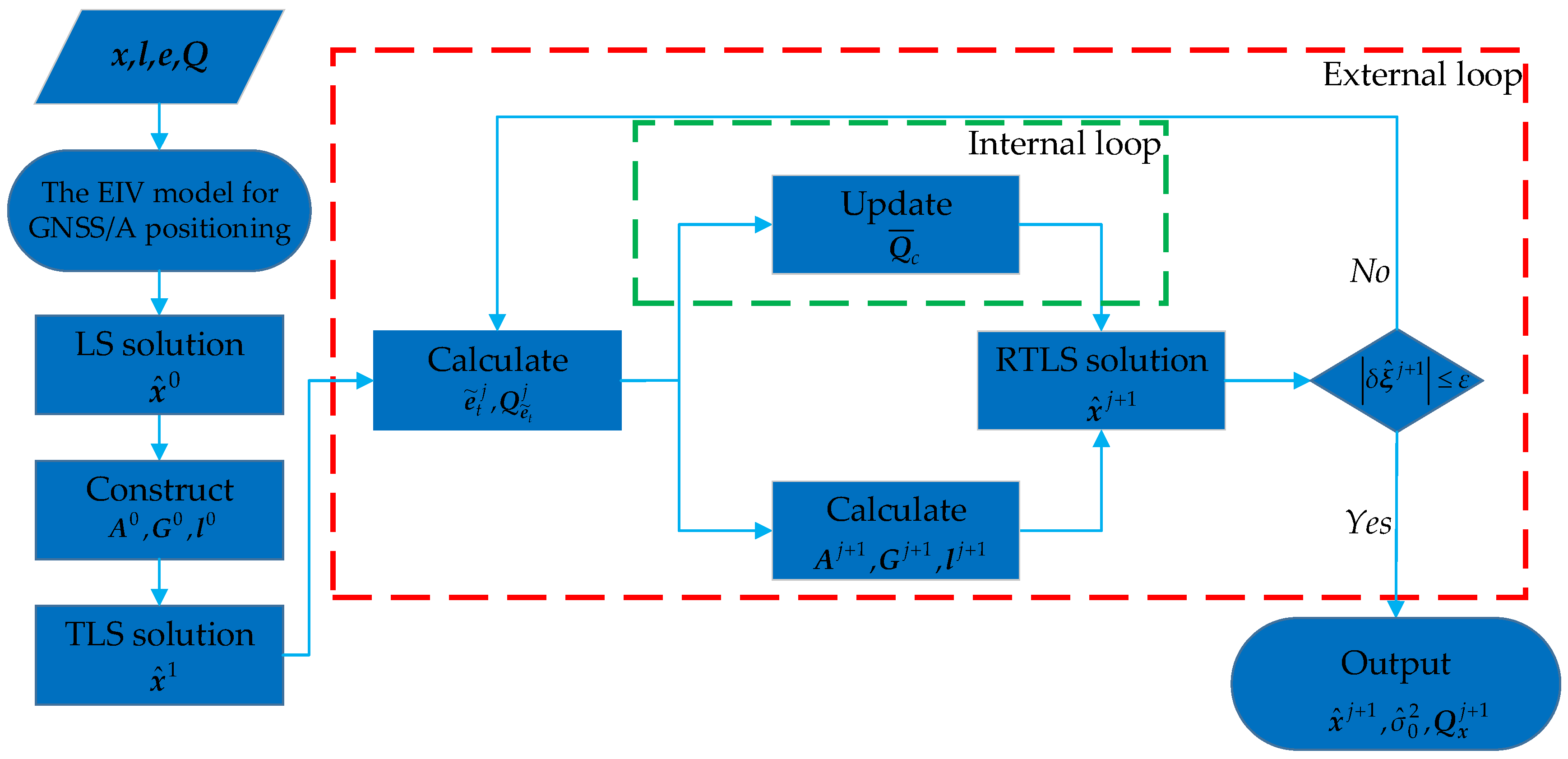
2.2. Robust Total Least-Squares Estimator for Seafloor Geodetic Control Point Positioning

Observations are inevitably affected by outliers, which does not change for the automated GNSS/A system. It is thus necessary to design a robust version of the TLS estimator to improve the reliability of underwater acoustic positioning. The M-estimator is a simple and attractive robust estimation method. It is simple because it is very convenient to be executed by the iteration method with variable weights; additionally, it is attractive because it shows excellent resistance to the unpatterned outliers. The M-estimator is to re-weigh acoustic observations based on predicted residuals to weaken or eliminate the adverse effect of suspicious acoustic observations or outliers. The capacity of residuals to precisely represent true errors is a critical determinant in the robustness of robust estimation algorithms. The utilization of standardized residuals and the robust variance factor of unit weight are two effective methodologies for enhancing the algorithm’s robustness [49]. Golub and van Loan point out that the TLS estimator is not suitable for residual prediction [52]. Different random quantities have serious hidden and blanking effects in each observation equation. Therefore, the design of robust estimation algorithms based on single-prediction residuals is not reasonable, to some extent.

The LS estimator is an effective method for residual prediction. Amiri-Simkooei and Jazaeri present a series of formulae for the EIV model based on the standard LS theory [42]. These linearly approximate formulae have forms that are similar to those of the LS estimator. The “total residuals” are expressed as

$${\tilde{\mathit{e}}}_t^{j+1}={\mathit{l}}^j-{\mathit{A}}^j\delta {\widehat{\mathsf{\xi }}}^{j+1}$$

(23)

and the corresponding co-factor matrix obtained by the co-factor propagation law is as follows [39,42]:

$${\mathit{Q}}_{{\tilde{\mathit{e}}}_t}^{j+1}={\mathit{Q}}_c-{\mathit{A}}^j{\left({{\mathit{A}}^j}^{\mathrm{T}}{\mathit{Q}}_c^{-1}{\mathit{A}}^j\right)}^{-1}{{\mathit{A}}^j}^{\mathrm{T}}$$

(24)

“Total residuals” are the predicted residuals’ combination of $\mathit{A}$ and $\mathit{y}$. To achieve excellent robustness in both observation and structure spaces, the standardized total residual should be used as follows

$${\tilde{v}}_{ti}^{j+1}={\displaystyle \frac{{\tilde{e}}_{ti}^{j+1}}{{\widehat{\sigma }}_0{Q}_{{\tilde{e}}_{ti}}^{j+1}}}$$

(25)

where ${\tilde{e}}_{ti}^{j+1}$ and $Q_{{\tilde{e}}_{ti}}^{j+1}$ represent the ith component of ${\tilde{\mathit{e}}}_t^{j+1}$ and the ith diagonal element of ${\mathit{Q}}_{{\tilde{\mathit{e}}}_t}^{j+1}$, respectively; ${\widehat{\sigma }}_0$ represents the posteriori standard deviation of unit weight, which can be estimated using the median method

$${\widehat{\sigma }}_0=1.4286\cdot \underset{i=1}{\overset{m}{\mathrm{med}}}\left(\left|{\displaystyle \frac{{\tilde{e}}_{ti}^{j+1}}{Q_{{\tilde{e}}_{ti}}^{j+1}}}\right|\right)$$

(26)

The RTLS estimator can be realized by the selection weight iteration method. ${\mathit{Q}}_{{\tilde{\mathit{e}}}_t}^{j+1}$ will be reconstructed based on ${\tilde{\mathit{v}}}_t^{j+1}$ from each successful TLS estimate. Here, the IGGIII equivalent weight function will be chosen, and the corresponding co-factor factor function is as follows:

$$R_i=\left\{\begin{array}{c}1,\left|{\tilde{v}}_{ti}^{j+1}\right|\le k_0\\ {\displaystyle \frac{\left|{\tilde{v}}_{ti}^{j+1}\right|}{k_0}}{\left({\displaystyle \frac{k_1-k_0}{k_1-\left|{\tilde{v}}_{ti}^{j+1}\right|}}\right)}^2,k_0<\left|{\tilde{v}}_{ti}^{j+1}\right|\le k_1\\ 10^{10},\left|{\tilde{v}}_{ti}^{j+1}\right|>k_1\end{array}\right.$$

(27)

where $R_i$ stands for the ith diagonal element of the co-factor factor matrix $\mathit{R}$. The co-factor function Equation (28) is a typical three-segment function, as follows: (1) $\left|{\tilde{v}}_{ti}^{j+1}\right|\le k_0$ is the conserved area, the RTLS estimator is the TLS estimator, and the normal observation equations are retained to improve the effectiveness of the parameter estimation method; (2) $k_0<\left|{\tilde{v}}_{ti}^{j+1}\right|\le k_1$ is an area of concern, and the suspicious observation equations will be re-weighted to reduce their adverse effect on parameter estimation based on predicted “total residuals”; (3) $k_1<\left|{\tilde{v}}_{ti}^{j+1}\right|$ is the exclusion area, and abnormal observation equations will be removed to eliminate their adverse effect. Here, a big number $10^{10}$ is used to replace infinity in practice. $k_0$ and $k_1$ are two experiential thresholds that are used to adjust the adaptability of the RLTS estimator. They are usually recommended as 2.0–3.0 and 4.5–8.5 according to the actual needs, respectively [49]. Therefore, the equivalent co-factor matrix ${\overline{\mathit{Q}}}_c$ is given as

$${\overline{\mathit{Q}}}_c=\sqrt{\mathit{R}}{\mathit{Q}}_c\sqrt{\mathit{R}}$$

(28)

thus, the posteriori estimate of the unit weight variance factor within the TLS principle is

$${\widehat{\sigma }}_0^2={\displaystyle \frac{{{\tilde{v}}_{ti}^{j+1}}^{\mathrm{T}}{\overline{\mathit{Q}}}_c^{-1}{\tilde{v}}_{ti}^{j+1}}{m-4-p}}$$

(29)

where $p$ is the number of observation equations falling into the exclusion area.

Figure 2 shows the implementation algorithm of the proposed RTLS estimator, named RTLS_Eqn. The proposed RTLS estimator can be achieved by the following two iterative loops: an internal loop to implement the re-weight operation and an external loop to implement the TLS estimator [39,42]. A detailed execution instruction of the proposed RTLS estimator is as follows:

• In the first iteration, the LS estimate ${\widehat{\mathit{x}}}^0$ is chosen as the initial value. In this case, GNSS positioning errors are ignored; that is, ${\tilde{\mathit{e}}}_x^0=0$. Then, ${\mathit{A}}^0$, ${\mathit{G}}^0$, and ${\mathit{l}}^0$ are constructed. The TLS estimate ${\widehat{\mathit{x}}}^1$ is calculated according to Equations (13) and (14), which is used to perform the subsequent robustness process.
• In the jth iteration, ${\tilde{\mathit{e}}}_t^j$ and ${\mathit{Q}}_{{\tilde{\mathit{e}}}_t}^j$ are calculated in terms of Equations (23) and (24). The re-weight operation Equations (25)–(28) can be conducted, and ${\overline{\mathit{Q}}}_c$ is calculated for the next TLS iteration.
• In terms of the previous iteration ${\widehat{\mathit{x}}}^j$, ${\mathit{A}}^{j+1}$, ${\mathit{G}}^{j+1}$, and ${\mathit{l}}^{j+1}$ are updated. The ${\mathit{Q}}_c$ should be replaced by its equivalent version ${\overline{\mathit{Q}}}_c$. The RTLS estimate ${\widehat{\mathit{x}}}^{j+1}$ is calculated according to Equations (13) and (14) for the next re-weight operation.
• If $\left|\delta {\widehat{\mathsf{\xi }}}^{j+1}\right|>\epsilon$, the termination condition is violated. The iteration steps (b) and (c) will be repeated; if $\left|\delta {\widehat{\mathsf{\xi }}}^{j+1}\right|\le \epsilon$, the termination condition is satisfied. The iteration process will be stopped, and then ${\widehat{\sigma }}_0^2$ and ${\mathit{Q}}_x^{j+1}$ can be calculated according to Equations (29) and (18).

3. Results

To validate the robustness and efficiency of the proposed RTLS algorithm, an emulational marine observation environment is constructed, and a series of different experimental scenarios at different depths are designed. A series of statistical indicators are used to compare the performance between the proposed RTLS algorithm and other related algorithms.

Assume that a single seafloor transponder is installed at the bottom of the ocean with a true coordinate $\left(\begin{array}{ccc}0& 0& -h\end{array}\right)$; $h$ stands for the simulated water depth. In recent years, China has carried out a lot of research on the marine PNT system, and then gradually constructed the marine PNT system for the exploration, development, and utilization of marine resources. Due to the large difference in water depths around China, we will choose several typical water depths for simulation experiments. The two typical water depths are predefined as 150 m and 3000 m, respectively. As shown in Figure 1, a station-centered Cartesian coordinate system is established. The z-axis is perpendicular to sea level and directed towards the zenith; the x-axis is parallel to sea level and directed towards the north; and the y-axis is parallel to sea level and directed towards the east. The surveying vessel sails along a symmetrical circular tracking line, precisely overhead of the seafloor transponder. To obtain the optimal geometrical configuration of the seafloor geodetic control point positioning, the radius of the circular tracking line is equal to $\sqrt{2}\cdot h$ [14].

The surveying vessel conducts acoustic ranging to collect 1080 observations at a speed of 4 nmile/h. As shown in Figure 3, because the true values of the acoustic ranging and incident angle are known, the Munk sound velocity profile is adopted, and then the constant-gradient ray tracking algorithm is reversely used to calculate the underwater propagation time of the acoustic ranging signals as final observations. The acoustic ranging value can be calculated by multiplying the sound travel time by the average sound speed based on the Munk sound velocity profile [21,50]. To ensure there has been enough data collection, multiple circle tracking lines are required in a shallow sea, while only one circle tracking line is needed in a deep sea. Circular sailing can effectively suppress the adverse effect of incidence angle variation during data processing [14]. The acoustic ranging error consists of the random error and systematic error. The random error is simulated through a normal distribution function $N\left(\mathrm{0,0.0}{5}^2\right)$, and the systematic error can be introduced according to [28], as follows:

$$\delta l_{vi}=c_1\sin \left(2\pi {\displaystyle \frac{{\left(t_i-t_0\right)}_{minute}}{T_w}}\right)+c_2\sin \left(2\pi {\displaystyle \frac{{\left(t_i-t_0\right)}_{hour}}{T_D}}\right)+c_3\left(1-e^{-{\displaystyle \frac{1}{2}}{\displaystyle \frac{f\left({\mathit{x}}_i,\mathit{x}\right)}{{\left(2km\right)}^2}}}\right)+c_4$$

(30)

Here, $t_0$ is the initial time. Assign those parameters in Equation (30), as follows: $c_1=0.12$ m, $T_w=20$ min, $c_2=0.2$ m, $T_w=12$ h, $c_3=2$ cm, and $c_4=0.1$ m. Equation (30) shows that the systematic error of acoustic ranging consists of four components. Component one and component two stand for the short-term period and long-term period caused by the variable of sound velocity, respectively; component three stands for the regional correlation term constructed by the Gaussian function; and component four stands for the constant term reflecting the large-scale influence of ocean activity. The typical accuracy of tracking point coordinates obtained by satellite-based differential positioning, PPP, RTK, or post-processing differential positioning varies from several centimeters to tens of centimeters. Referring to this typical positioning accuracy, the accuracy of horizontal and vertical coordinate components is assumed to be 10 cm and 20 cm, respectively. The ocean wave is also modeled based on a cosine function with an amplitude of 2 m and a period of 15 s to formally simulate the actual marine environment.

Here, the following three comparative evaluation schemes are conducted as follows:

a.

The TLS estimator is carried out, which is used as a reference to verify the effectiveness of other methods [39,42]. Considering the random errors of tracking point coordinates, the TLS estimator is a more optimal parameter estimation method for the seafloor geodetic control point positioning [38,50].

b.

The RTLS estimator is designed based on M-estimation, where the re-weighting operation is achieved according to each of the individual-predicted residuals. Here, it is referred to as RTLS_Obs [49,50].

c.

The RTLS estimator, RTLS_Eqn, is the algorithm proposed in this paper, which is also a robust estimation algorithm based on M-estimation and achieved by re-weighting “total residuals”.

Assume that six percent of the random quantities are contaminated by outliers within the EIV model. Then, three different scales of outliers, generated by uniform distribution, are added in terms of their ratio to random errors, and their value intervals are (unit: m) as follows: (1) $\left[\begin{array}{cc}0.4& 1\end{array}\right]$, which is defined as “small outliers”; (2) $\left[\begin{array}{cc}1& 10\end{array}\right]$, which is defined as “medium outliers”; and (3) $\left[\begin{array}{cc}10& 100\end{array}\right]$, which is defined as “large outliers”. According to the above experimental environment, the Monte Carlo simulation will be repeated 1000 times under different contamination schemes. The purpose of these Monte Carlo simulations is to understand how the estimate of the seafloor geodetic control point, obtained by the above-mentioned estimation methods, differs from its true value. The 3D deviation of the seafloor geodetic control point can be calculated by

$$\Delta x_k=\sqrt{{\left(n_t^k-n_t^0\right)}^2+{\left(e_t^k-e_t^0\right)}^2+{\left(u_t^k-u_t^0\right)}^2},k=1,...,1000$$

(31)

One can use the following four indicators to evaluate the above estimation methods, namely the Root Mean Square Error (RMSE)

$$\mathrm{RMSE}(\mathsf{\Delta }x)=\sqrt{{\displaystyle \frac{1}{1000}}\sum _{k=1}^{1000}{\left(\Delta x_k\right)}^2},k=1,...1000,$$

(32)

the standard deviation (STD)

$$\mathrm{STD}(\mathsf{\Delta }x)=\sqrt{{\displaystyle \frac{1}{1000-1}}\sum _{k=1}^{1000}(\Delta x_k-\Delta \overline{x}{)}^2},k=1,...,1000,$$

(33)

the maximum (MAX)

$$\mathrm{STD}(\mathsf{\Delta }x)=\sqrt{{\displaystyle \frac{1}{1000-1}}\sum _{k=1}^{1000}(\Delta x_k-\Delta \overline{x}{)}^2},k=1,...,1000,$$

(34)

and the minimum (MIN)

$$\mathrm{MIN}\left(\mathsf{\Delta }x\right)=\mathrm{minimum}\left(\left|\Delta x_k\right|\right),k=1,...,1000$$

(35)

Here, $\left(\overline{\cdot }\right)$ represent the average value of the corresponding parameter. The RMSE intuitively evaluates the deviation between the estimated value and the true value. Significantly, it can be broken down into the following two parts

$$\mathrm{RMS}{\mathrm{E}}^2\left(\Delta x\right)=\mathrm{ST}{\mathrm{D}}^2\left(\Delta x\right)+(\Delta \overline{x}-0{)}^2$$

(36)

That is, this deviation evaluates the comprehensive effect of estimated stability and system bias. Our goal is to obtain a higher estimated stability and a lower system bias, namely a small RMSE. Next, we apply the above three estimation methods to calculate the estimates under normal random errors and various contamination schemes. The final statistical results are shown in

Table 1. The statistics and average iteration time of different methods under the influence of random errors.

Depth (m)	Method	MAX	MIN	RMSE	STD	Time (s)
150	TLS	0.1264	0.0044	0.0820	0.0413	10.1381
	RTLS_Obs	0.1264	0.0044	0.0839	0.0433	13.4279
	RTLS_Eqn	0.1264	0.0044	0.0831	0.0420	12.2871
3000	TLS	0.1363	0.0058	0.0893	0.0519	7.0651
	RTLS_Obs	0.1363	0.0058	0.0909	0.0532	9.6812
	RTLS_Eqn	0.1363	0.0058	0.0901	0.0521	9.0032

,

Table 2. The statistics and average iteration time of different methods under the contamination of small outliers.

Depth (m)	Method	MAX	MIN	RMSE	STD	Time (s)
150	TLS	0.7532	0.0316	0.2932	0.1423	10.3877
	RTLS_Obs	0.3701	0.0150	0.1832	0.0874	29.5954
	RTLS_Eqn	0.3219	0.0126	0.1503	0.0692	23.5892
3000	TLS	0.7743	0.0378	0.3768	0.1698	7.2562
	RTLS_Obs	0.4520	0.0181	0.2210	0.1102	18.3284
	RTLS_Eqn	0.3923	0.0162	0.1912	0.0951	12.3018

,

Table 3. The statistics and average iteration time of different methods under the contamination of medium outliers.

Depth (m)	Method	MAX	MIN	RMSE	STD	Time (s)
150	TLS	2.5231	0.0633	0.9726	0.4032	16.3852
	RTLS_Obs	0.2498	0.0078	0.1132	0.0498	21.3239
	RTLS_Eqn	0.2100	0.0066	0.1029	0.0432	12.5201
3000	TLS	2.7143	0.2361	1.1823	0.5478	13.9018
	RTLS_Obs	0.2645	0.0099	0.1293	0.0537	15.3058
	RTLS_Eqn	0.2569	0.0085	0.1201	0.0509	9.8326

and

Table 4. The statistics and average iteration time of different methods under the contamination of large outliers.

Depth (m)	Method	MAX	MIN	RMSE	STD	Time (s)
150	TLS	4.3217	0.3334	1.7256	0.8726	37.9442
	RTLS_Obs	0.6734	0.1824	0.3304	0.1632	35.2499
	RTLS_Eqn	0.5833	0.1666	0.2987	0.1543	24.4930
3000	TLS	6.9732	0.4918	2.3613	1.2109	26.0511
	RTLS_Obs	0.8291	0.2472	0.3789	0.1845	20.3294
	RTLS_Eqn	0.7119	0.2092	0.3400	0.1726	13.4010

.

4. Discussion

Table 1 shows the statistics, MAX, MIN, RMSE, and STD, and the average iteration time of Monte Carlo simulation experiments obtained by three parameter estimation methods under the influence of random errors in a shallow sea of 150 m and a deep sea of 3000 m, respectively. Because the random errors of tracking point coordinates and acoustic ranging observations are considered simultaneously, the TLS estimator is more suitable for the seafloor geodetic control point positioning. When the random quantities are not contaminated by outliers, the TLS estimator achieves the optimal estimate. That is, the RMSE produced by the TLS estimator is the smallest, and it is the most efficient parameter estimation method, with the smallest STD. In the normal error situation, two robust techniques, the RTLS_Obs estimator and the RTLS_Eqn estimator, behave just as well as the TLS estimator, according to the statistics, whereas their RMSE and STD increase, but not dramatically. The final positioning accuracy obtained by the three above-mentioned estimation methods can reach the centimeter level. It should also be noted that the average iteration time of two robust techniques does increase significantly. This is due to the fact that some normal random quantities are misjudged as outliers, and therefore the re-weighting operation is performed. For the normal observations, performing a robust estimation will reduce the effectiveness of parameter estimation and finally result in the larger RMSE.

Table 2, Table 3 and Table 4 further show the statistics and the average iteration time of Monte Carlo simulation experiments, when the random quantities are contaminated by the outliers of different scales and do not strictly follow the normal error distribution. For the non-normal error distribution, the TLS estimate deviates considerably from its true value, and further causes the large RMSE. The final positioning accuracy will degrade to the decimeter level or even the meter level with the outliers of different scales. Meanwhile, the effectiveness of the TLS estimator is significantly reduced, because there are no measures to inhibit the adverse effect of outliers. The TLS estimator breaks down systematically at these contaminated simulations and loses its excellent statistical properties. As the outliers become larger, the average iteration time of the TLS estimator also grows, and the TLS estimator becomes poorer due to those deteriorating normal equations. For the small or medium outliers, the average iteration time of the TLS estimator has not increased significantly, but for the large outliers, it even exceeds two robust techniques that require re-weighting. This shows that those untreated outliers will also worsen normal equation solving. The TLS estimator is not suitable for the contaminated data.

The poor positioning of the TLS estimator demonstrates that the accuracy of the seafloor geodetic control point positioning will be greatly weakened when tracking point coordinates and/or when acoustic ranging observations are contaminated by outliers. Therefore, it is very necessary to introduce a robust substitute to eliminate or reduce the adverse effect of outliers. Table 2, Table 3 and Table 4 also present the performance of two robust technologies in an all-round way. In the presence of outliers for random variables, one can find that two robust technologies are still quite good compared to the TLS estimator. All of the final positioning accuracy obtained by two robust technologies can still hold decimeter levels for the outliers of different scales. By performing the re-weighting operation, the RMSE values of the RTLS_Eqn estimator are averagely improved by 73.62% and 74.90%, compared to the TLS estimator in a shallow sea of 150 m and a deep sea of 3000 m, respectively. Furthermore, the STD values are averagely improved by 74.33% and 73.48%, respectively. The adverse effects of abnormal random equations or outliers are effectively suppressed. The re-weighting operation can also greatly improve the effectiveness of parameter estimation under the contamination of outliers. By re-weighting based on “total residuals”, the RMSE values of the RTLS_Eqn estimator are averagely improved by 12.22% and 10.27%, compared to the RTLS_Obs estimator in a shallow sea of 150 m and a deep sea of 3000 m, respectively. Furthermore, the STD values are averagely improved by 13.17% and 8.45%, respectively. This shows that re-weighting based on “total residuals” can identify abnormal observation equations damaged by outliers more effectively and improve the effectiveness of robust estimation methods. The RTLS_Eqn estimator achieves the optimal parameter estimation among the three above-mentioned estimation methods for the contaminated data. The RTLS_Eqn estimator reduces the number of re-weighting and enhances the ability to identify abnormal observation equations or outliers. Therefore, its average iteration time is averagely improved by 30.70% and 34.24% compared to the RTLS_Obs estimator in a shallow sea of 150 m and a deep sea of 3000 m, respectively. One cannot expect that two robust technologies behave just as well as the TLS estimator under the influence of random errors. Because the outliers still have an adverse effect (which may be very small), the elimination of abnormal observation equations will further reduce the effectiveness of robust estimation methods. For the outliers of different scales, two robust technologies show different robustness abilities. Compared to the contamination of small outliers, two robust technologies have improved the robustness and effectiveness and reduced the average iteration time under the contamination of medium outliers, as shown in Table 2 and Table 3. This indicates that small outliers are more difficult to find, and they affect the performance of robust estimation methods. Table 4 shows that there is a significant decline in the statistical performance of two robust technologies for the large outliers. This is because it is easy to form leverage observation equations under the contamination of large outliers.

The TLS estimator and its robust substitutes perform the deregularizing operation during execution, which will affect their numerical stability and even lead to calculation failure. This is an important challenge in adopting them for data processing. Although all of the three above-mentioned parameter estimation methods introduce an additional parameter related to the ranging systematic error and consider the random errors of tracking point coordinates, there are still significant estimation biases in their estimates with/without the contamination of outliers. This is due to the unreasonable modeling of the systematic error, and/or the coupling effect between the systematic error and random error. The acoustic ranging error is still the main error source for the seafloor geodetic control point positioning. The overall conclusion of these Monte Carlo simulation experiments is that the RTLS_Eqn estimator achieves its design objective. It can obtain reasonable parameter estimates in normal situations, and is also able to more effectively suppress the adverse effect of outliers in abnormal situations.

5. Conclusions

The marine PNT system is an important marine infrastructure for resource protection, scientific research, and economic development. The GNSS/A technique is the main method for building the marine PNT system. The tracking point coordinates are inevitably affected by positioning errors from various real-time or post-processing GNSS positioning processes. The EIV model and the TLS estimator are more suitable for modeling and data processing of the seafloor geodetic control point positioning. However, the random quantities, including tracking point coordinates and acoustic ranging observations, may be affected by outliers. The TLS estimator minimizes the quadratic sum of all of the orthogonal residuals. This optimization criterion is particularly susceptible to outliers. To cope with this thorny problem, we propose the RTLS_Eqn estimator, which holds robustness in both observation and structure spaces. This RTLS estimation algorithm is expected to have a better performance than the existing related methods. Finally, the Monte Carlo simulation experiments are used for data analysis, and the main conclusions are as follows:

a.

When considering the random errors of tracking point coordinates and acoustic ranging observations simultaneously, the TLS estimator achieves the optimal estimate of the seafloor geodetic control point for the normally distributed errors, but two robust techniques also performed quite well. Meanwhile, the RTLS_Eqn estimator is slightly better than the RTLS_Obs estimator according to the statistics and the average iteration time. The robust estimation methods are not recommended for the non-contaminated data.

b.

For the abnormal situation, we arrive at the conclusions that we expect, in which the TLS estimator loses its statistical optimality and breaks down systematically because it minimizes the quadratic sum of orthogonal residuals and cannot limit the influence of outliers. The introduction of robust substitutions can effectively suppress the adverse effect of outliers. Please note that the RTLS_Obs estimator based on single-predicted residuals has some defects and cannot effectively identify outliers. We use “total residuals” instead of single residuals for re-weighting to design the RTLS_Eqn estimator, which shows better robustness and effectiveness. The scale of outliers is also an important factor affecting the performance of robust estimation methods. Small outliers may be confused with random errors, and large outliers may bring the risk of leverage observation, which will degrade the performance of robust estimation methods. To conclude, the RTLS_Eqn estimator achieves its design objective, which is a more reliable robust estimation method according to the statistics and the average iteration time.

c.

The TLS estimator and its robust substitutions still have the possibility of iteration failure because of the deregularizing operation. How the ranging systematic error is handled is a key factor in determining the positioning accuracy of the seafloor geodetic control point.

References

1. Yang, Y. Concepts of Comprehensive PNT and Related Key Technologies. Acta Geod. Cartogr. Sin. 2016, 45, 505–510. [Google Scholar] [CrossRef]
2. Altamimi, Z.; Rebischung, P.; Métivier, L.; Collilieux, X. ITRF2014: A New Release of the International Terrestrial Reference Frame Modeling Nonlinear Station Motions: ITRF2014. J. Geophys. Res. Solid Earth 2016, 121, 6109–6131. [Google Scholar] [CrossRef]
3. Altamimi, Z.; Rebischung, P.; Collilieux, X.; Métivier, L.; Chanard, K. ITRF2020: An Augmented Reference Frame Refining the Modeling of Nonlinear Station Motions. J. Geod. 2023, 97, 47. [Google Scholar] [CrossRef]
4. Poutanen, M.; Rózsa, S. The Geodesist’s Handbook 2020. J. Geod. 2020, 94, 109. [Google Scholar] [CrossRef]
5. Spiess, F.N.; Chadwell, C.D.; Hildebrand, J.A.; Young, L.E.; Purcell, G.H.; Dragert, H. Precise GPS/Acoustic Positioning of Seafloor Reference Points for Tectonic Studies. Phys. Earth Planet. Inter. 1998, 108, 101–112. [Google Scholar] [CrossRef]
6. Gagnon, K.; Chadwell, C.D.; Norabuena, E. Measuring the Onset of Locking in the Peru–Chile Trench with GPS and Acoustic Measurements. Nature 2005, 434, 205–208. [Google Scholar] [CrossRef]
7. Fujita, M.; Ishikawa, T.; Mochizuki, M.; Sato, M.; Toyama, S.; Katayama, M.; Kawai, K.; Matsumoto, Y.; Yabuki, T.; Asada, A.; et al. GPS/Acoustic Seafloor Geodetic Observation: Method of Data Analysis and Its Application. Earth Planet Space 2006, 58, 265–275. [Google Scholar] [CrossRef]
8. Sousa, R.; Alcocer, A.; Oliveira, P.; Ghabcheloo, R.; Pascoal, A. Joint Positioning and Navigation Aiding System for Underwater Robots. In Proceedings of the OCEANS 2008, Quebec City, QC, Canada, 15–18 September 2008; pp. 1–8. [Google Scholar]
9. Chadwell, C.D.; Spiess, F.N. Plate Motion at the Ridge-transform Boundary of the South Cleft Segment of the Juan de Fuca Ridge from GPS-Acoustic Data. J. Geophys. Res. 2008, 113, 2007JB004936. [Google Scholar] [CrossRef]
10. Chen, H.-H.; Wang, C.-C. Accuracy Assessment of GPS/Acoustic Positioning Using a Seafloor Acoustic Transponder System. Ocean Eng. 2011, 38, 1472–1479. [Google Scholar] [CrossRef]
11. Osada, Y.; Fujimoto, H.; Miura, S.; Sweeney, A.; Kanazawa, T.; Nakao, S.; Sakai, S.; Hildebrand, J.A.; Chadwell, C.D. Estimation and Correction for the Effect of Sound Velocity Variation on GPS/Acoustic Seafloor Positioning: An Experiment off Hawaii Island. Earth Planet Space 2014, 55, e17–e20. [Google Scholar] [CrossRef]
12. Ribeiro, F.J.L.; de Castro Pinto Pedroza, A.; Costa, L.H.M.K. Underwater Monitoring System for Oil Exploration Using Acoustic Sensor Networks. Telecommun. Syst. 2015, 58, 91–106. [Google Scholar] [CrossRef]
13. DeSanto, J.B.; Sandwell, D.T.; Chadwell, C.D. Seafloor Geodesy from Repeated Sidescan Sonar Surveys. JGR Solid Earth 2016, 121, 4800–4813. [Google Scholar] [CrossRef]
14. Yang, Y.; Xu, T.; Xue, S. Progresses and Prospects in Developing Marine Geodetic Datum and Marine Navigation of China. Acta Geod. Cartogr. Sin. 2017, 46, 1–8. [Google Scholar] [CrossRef]
15. Sakic, P.; Ballu, V.; Royer, J.-Y. A Multi-Observation Least-Squares Inversion for GNSS-Acoustic Seafloor Positioning. Remote Sens. 2020, 12, 448. [Google Scholar] [CrossRef]
16. Yang, Y.; Qin, X. Resilient Observation Models for Seafloor Geodetic Positioning. J. Geod. 2021, 95, 79. [Google Scholar] [CrossRef]
17. Sun, Z.; Wang, Z.; Nie, Z.; Jia, C.; Shan, R. A New Angle-Calibration Method for Precise Ultra-Short Baseline Underwater Positioning. Remote Sens. 2024, 16, 2584. [Google Scholar] [CrossRef]
18. Spiess, F. Suboceanic Geodetic Measurements. IEEE Trans. Geosci. Remote Sens. 1985, GE-23, 502–510. [Google Scholar] [CrossRef]
19. Zhou, P.; Xiao, G.; Du, L. Initial Performance Assessment of Galileo High Accuracy Service with Software-Defined Receiver. GPS Solut. 2024, 28, 2. [Google Scholar] [CrossRef]
20. Wei, H.; Xiao, G.; Zhou, P.; Li, P.; Xiao, Z.; Zhang, B. Combining Galileo HAS and Beidou PPP-B2b with Helmert Coordinate Transformation Method. GPS Solut. 2025, 29, 35. [Google Scholar] [CrossRef]
21. Zhao, S.; Wang, Z.; Nie, Z.; He, K.; Ding, N. Investigation on Total Adjustment of the Transducer and Seafloor Transponder for GNSS/Acoustic Precise Underwater Point Positioning. Ocean Eng. 2021, 221, 108533. [Google Scholar] [CrossRef]
22. Sato, M.; Fujita, M.; Matsumoto, Y.; Saito, H.; Ishikawa, T.; Asakura, T. Improvement of GPS/Acoustic Seafloor Positioning Precision through Controlling the Ship’s Track Line. J. Geod. 2013, 87, 825–842. [Google Scholar] [CrossRef]
23. Chen, G.; Liu, Y.; Liu, Y.; Liu, J. Improving GNSS-Acoustic Positioning by Optimizing the Ship’s Track Lines and Observation Combinations. J. Geod. 2020, 94, 61. [Google Scholar] [CrossRef]
24. Xue, S.; Yang, Y.; Yang, W. Single-Differenced Models for GNSS-Acoustic Seafloor Point Positioning. J. Geod. 2022, 96, 38. [Google Scholar] [CrossRef]
25. Fox, C.G. Five Years of Ground Deformation Monitoring on Axial Seamount Using a Bottom Pressure Recorder. Geophys. Res. Lett. 1993, 20, 1859–1862. [Google Scholar] [CrossRef]
26. Ballu, V.; Bouin, M.-N.; Calmant, S.; Folcher, E.; Bore, J.-M.; Ammann, J.; Pot, O.; Diament, M.; Pelletier, B. Absolute Seafloor Vertical Positioning Using Combined Pressure Gauge and Kinematic GPS Data. J. Geod. 2010, 84, 65–77. [Google Scholar] [CrossRef]
27. Yang, F.; Lu, X.; Li, J.; Han, L.; Zheng, Z. Precise Positioning of Underwater Static Objects without Sound Speed Profile. Mar. Geod. 2011, 34, 138–151. [Google Scholar] [CrossRef]
28. Xu, P.; Ando, M.; Tadokoro, K. Precise Three-Dimensional Seafloor Geodetic Deformation Measurements Using Difference Techniques. Earth Planet Space 2005, 57, 795–808. [Google Scholar] [CrossRef]
29. Wang, L.; Yu, H.; Chen, X. An Algorithm for Partial EIV Model. Acta Geod. Cartogr. Sin. 2016, 45, 22–29. [Google Scholar] [CrossRef]
30. Wang, L.; Xu, G.; Wen, G. A Method for Partial EIV Model with Correlated Observations. Acta Geod. Cartogr. Sin. 2017, 46, 978–987. [Google Scholar] [CrossRef]
31. Teunissen, P.J.G. Adjustment Theory: An Introduction; Delft University Press: Delft, The Netherlands, 2000. [Google Scholar]
32. Liu, Y.; Xue, S.; Qu, G.; Lu, X.; Qi, K. Influence of the Ray Elevation Angle on Seafloor Positioning Precision in the Context of Acoustic Ray Tracing Algorithm. Appl. Ocean Res. 2020, 105, 102403. [Google Scholar] [CrossRef]
33. Wang, Z.; Zhao, S.; Ji, S.; He, K.; Nie, Z.; Liu, H.; Shan, R. Real-Time Stochastic Model for Precise Underwater Positioning. Appl. Acoust. 2019, 150, 36–43. [Google Scholar] [CrossRef]
34. Sun, Z.; Wang, Z.; Nie, Z. A Stochastic Model for Precise GNSS/Acoustic Underwater Positioning Based on Transmission Loss of Signal Intensity. GPS Solut. 2023, 27, 202. [Google Scholar] [CrossRef]
35. Van Huffel, S.; Vandewalle, J. The Total Least Squares Problem: Computational Aspects and Analysis; Society for Industry and Applied Mathematics: Philadelphia, PA, USA, 1999. [Google Scholar]
36. Gong, X.; Hou, Z.; Wan, Y.; Zhong, Y.; Zhang, M.; Lv, K. Multispectral and SAR Image Fusion for Multiscale Decomposition Based on Least Squares Optimization Rolling Guidance Filtering. IEEE Trans. Geosci. Remote Sens. 2024, 62, 1–20. [Google Scholar] [CrossRef]
37. Schaffrin, B.; Wieser, A. On Weighted Total Least-Squares Adjustment for Linear Regression. J. Geod. 2008, 82, 415–421. [Google Scholar] [CrossRef]
38. Fang, X. Weighted Total Least Squares Solutions for Applications in Geodesy. Ph.D. Dissertation, Leibniz University Hannover, Hannover, Germany, 2011. [Google Scholar]
39. Fang, X. Weighted Total Least Squares: Necessary and Sufficient Conditions, Fixed and Random Parameters. J. Geod. 2013, 87, 733–749. [Google Scholar] [CrossRef]
40. Fang, X. A Structured and Constrained Total Least-Squares Solution with Cross-Covariances. Stud. Geophys. Geod. 2014, 58, 1–16. [Google Scholar] [CrossRef]
41. Fang, X. On Non-Combinatorial Weighted Total Least Squares with Inequality Constraints. J. Geod. 2014, 88, 805–816. [Google Scholar] [CrossRef]
42. Amiri-Simkooei, A.R.; Jazaeri, S. Weighted Total Least Squares Formulated by Standard Least Squares Theory. J. Geod. Sci. 2012, 2, 113–124. [Google Scholar] [CrossRef]
43. Wang, L.; Zhao, Y. Unscented Transformation with Scaled Symmetric Sampling Strategy for Precision Estimation of Total Least Squares. Stud. Geophys. Geod. 2017, 61, 385–411. [Google Scholar] [CrossRef]
44. Wang, L.; Wen, G. Non-Negative Least Squares Variance Component Estimation of Partial EIV Model. Acta Geod. Cartogr. Sin. 2017, 46, 857–865. [Google Scholar]
45. Wang, L.; Xu, G. Variance Component Estimation for Partial Errors-in-Variables Models. Stud. Geophys. Geod. 2016, 60, 35–55. [Google Scholar] [CrossRef]
46. Duchnowski, R.; Wyszkowska, P. Robust Procedures in Processing Measurements in Geodesy and Surveying: A Review. Meas. Sci. Technol. 2024, 35, 052002. [Google Scholar] [CrossRef]
47. Zhao, S.; Wang, Z.; Liu, H. Investigation on Underwater Positioning Stochastic Model Based on Sound Ray Incidence Angle. Acta Geod. Cartogr. Sin. 2018, 47, 1280–1289. [Google Scholar]
48. Dou, J.; Xu, B.; Dou, L. Robust GNSS Positioning Using Unbiased Finite Impulse Response Filter. Remote Sens. 2023, 15, 4528. [Google Scholar] [CrossRef]
49. Wang, B.; Li, J.; Liu, C. A Robust Weighted Total Least Squares Algorithm and Its Geodetic Applications. Stud. Geophys. Geod. 2016, 60, 177–194. [Google Scholar] [CrossRef]
50. Kuang, Y.; Lu, Z.; Wang, F.; Yang, K.; Li, L. A Nonlinear Gauss-Helmert Model and Its Robust Solution for Seafloor Control Point Positioning. Mar. Geod. 2023, 46, 16–42. [Google Scholar] [CrossRef]
51. Gong, X.; Wang, H.; Lu, T.; You, W.; Zhang, R. Combined Prediction Model for High-Speed Railway Bridge Pier Settlement Based on Robust Weighted Total Least-Squares Autoregression and Adaptive Dynamic Cubic Exponential Smoothing. J. Surv. Eng. 2023, 149, 04023001. [Google Scholar] [CrossRef]
52. Golub, G.H.; van Loan, C.F. An Analysis of the Total Least Squares Problem. SIAM J. Numer. Anal. 1980, 17, 883–893. [Google Scholar] [CrossRef]
Figure 1. Principle of GNSS/A underwater positioning.
Remotesensing 17 00276 g001
Figure 2. The flowchart of RTLS_Eq for GNSS/A underwater positioning.
Remotesensing 17 00276 g002
Figure 3. Munk sound velocity profile.
Remotesensing 17 00276 g003