Article

Downscaling Method for Crop Yield Statistical Data Based on the Standardized Deviation from the Mean of the Comprehensive Crop Condition Index

1
State Key Laboratory of Efficient Utilization of Arable Land in China, Institute of Agricultural Resources and Regional Planning, Chinese Academy of Agricultural Sciences, Beijing 100081, China
2
Key Laboratory of Agricultural Remote Sensing, Ministry of Agriculture and Rural Affairs, Institute of Agricultural Resources and Regional Planning, Chinese Academy of Agricultural Sciences, Beijing 100081, China
*
Author to whom correspondence should be addressed.
Remote Sens. 2025, 17(20), 3408; https://doi.org/10.3390/rs17203408
Submission received: 30 August 2025 / Revised: 9 October 2025 / Accepted: 10 October 2025 / Published: 11 October 2025
(This article belongs to the Special Issue Near Real-Time (NRT) Agriculture Monitoring)

Highlights

What are the main findings?
  • A downscaling method using the standardized deviation of the CCCI was proposed to effectively transform crop yield statistics from administrative units to the pixel level.
  • The spatial heterogeneity of crop growth was expressed through the spatiotemporal dynamic weights of CCCI, and the spatial variation in crop yield was effectively reflected.
What is the implication of the main finding?
  • This method provides reliable spatialized yield data to support crop yield predictions, climate change impact assessments, and precision agriculture applications at large scales.
  • Spatialized crop yield results could expand training samples for pixel-level yield predictions, overcoming the challenge of limited ground-truth data in agricultural remote sensing research.

Abstract

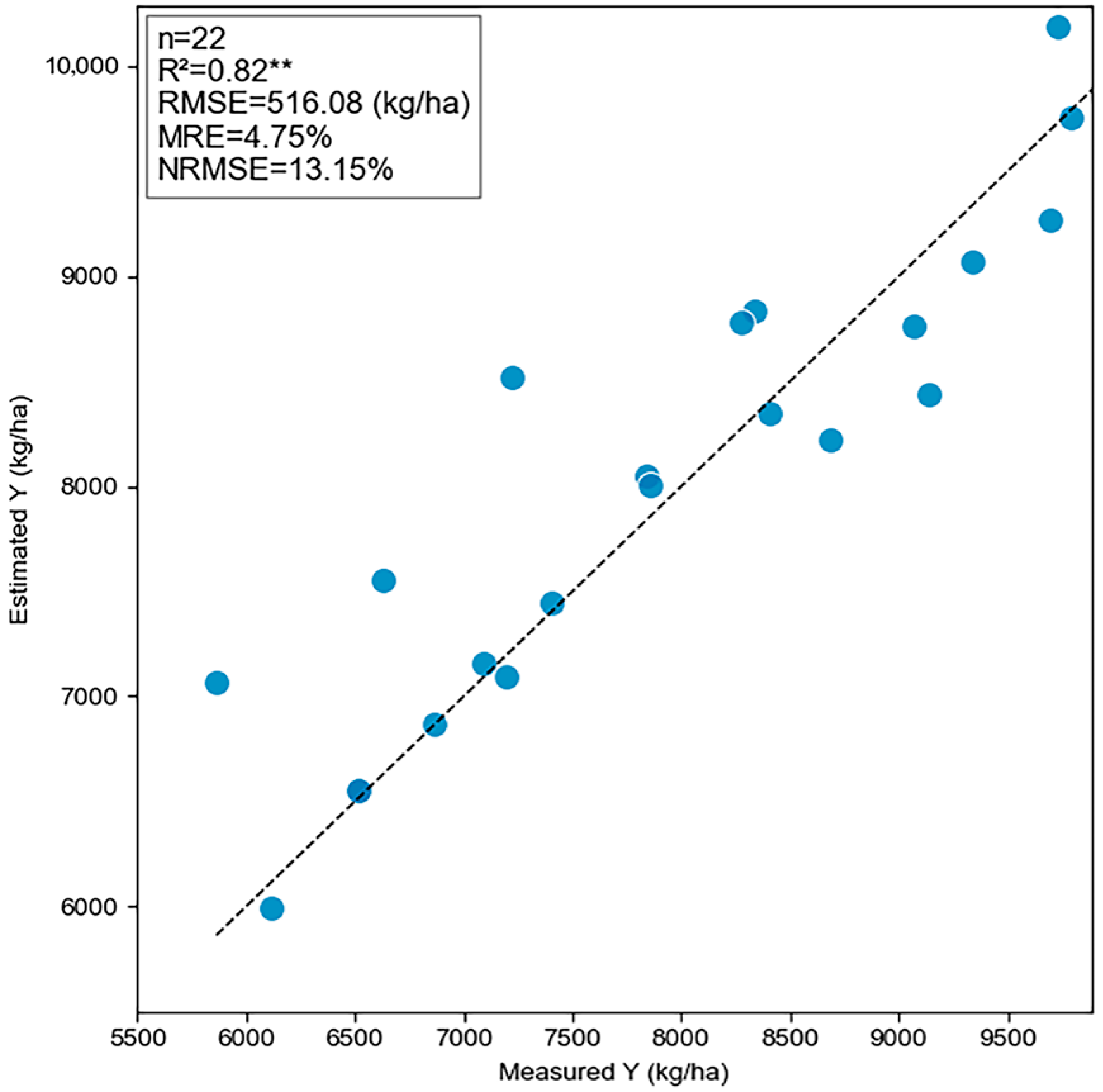
Spatializing crop yield statistical data with administrative divisions as the basic unit helps reveal the spatial distribution characteristics of crop yield and provides necessary spatial information to support field management and government decision-making. However, owing to an insufficient understanding of the factors affecting yield, accurately depicting its spatial differences remains challenging. Taking Hailun city, Heilongjiang Province, as an example, this study proposes a yield downscaling method based on the standardized deviation from the mean of the comprehensive crop condition index (CCCI) during key phenological periods of the growing season. First, Sentinel-2 remote sensing data were used to retrieve crop condition parameters during key phenological periods, and the CCCI was constructed using the correlation between crop condition parameters in key phenological periods and statistical yield as the weight. Subsequently, regression analysis and the entropy weight method were applied to determine the spatiotemporal dynamic weights of the CCCI during key phenological stages and to calculate the standardized deviation from the mean. By combining these two components, the comprehensive spatial difference index of the crop growth condition (CSDICGC) was derived, which offered a new way to characterize the discrepancies between the pixel-level yield and statistical yield, thereby downscaling the yield statistical data from the administrative unit to the pixel scale. The results indicated that this method achieved a regional accuracy close to 100%, with a strong fit at the pixel scale. Pixel-level accuracy validation against ground-truth maize yield data resulted in an R2 of 0.82 and a mean relative error (MRE) of 4.75%. The novelty of this study was characterized by the integration of multistage crop condition parameters with dynamic spatiotemporal weighting to overcome the limitations of single-index methods. The crop yield statistical data downscaling spatialization method proposed in this paper is simple and efficient and has the potential to be popularized and applied over relatively large regions.

1. Introduction

Crop statistical data (such as crop planting area and crop yield) are core indicators for assessing a country’s grain production capacity. With the increasing contribution rate of crop yield to grain production, crop yield improvements have become a key driving force for enhancing national food production capacity [1,2]. However, statistical yield data in most countries are still limited to county-level tabular records, which fail to reveal the true spatial distribution and variability of crop yields within administrative regions. This limitation greatly restricts the application of crop yield statistics in geographic research and decision-making [3,4]. Pixel-scale yield information not only resolves the contradiction between the spatial heterogeneity of agricultural production factors and the intraregional homogeneity of statistical data [5,6] but also serves as reliable sample data to meet the increasing data demands for field management, yield forecasting, and government decision-making.
Spatialization methods can supplement or refine spatial information by establishing spatial relationships among factors, thereby transforming statistical data from the administrative-unit scale to the grid scale. Compared with spatialization studies of socioeconomic data (e.g., population [7] and GDP [8]), agricultural statistical data spatialization has focused primarily on crop planting areas [9,10] and agricultural inputs [11,12], while research on crop production—particularly crop yield per unit area—remains limited. This scarcity is largely due to the sensitivity of crop yields to multiple factors, such as topography [13], climate [14], soil [15], and hydrology [16], which complicates spatialization. Early studies often adopted direct assignment methods, in which statistical yield data were simply converted into raster datasets. However, such approaches fail to address the issue of internal homogeneity of yield statistics within administrative units [17].
With the development of computer, information, and geospatial technologies, research on crop yield spatialization has advanced in recent years, and the main methods can generally be divided into direct and indirect approaches. Direct methods use spatially heterogeneous ancillary data as allocation weights to distribute regional yield statistics to grids. For instance, You et al. [18,19] coupled biophysical and anthropogenic factors and applied the ratio of potential yield within a grid to the regional average potential yield as a weighting coefficient, thereby producing global grid-scale yield distribution data for major crops. Zhu et al. [20] allocated county-level statistical yields to the pixel scale using normalized difference vegetation index (NDVI) time series data. However, the accuracy of direct approaches remains constrained by the spatial resolution of the input data. In contrast, indirect methods use certain methods or parameters to construct yield estimation models at the regional scale and apply them at the grid scale; then, regional statistical yields are used as a constraint to correct the spatialized results. For example, Liu et al. [5] developed a regression model between land use data and population density to produce a 1 km × 1 km distribution map of China’s grain yield. Li et al. [21] developed the GCYS model to quantify and spatialize integrated agricultural systems, converting grain crop yields from the county scale to the grid scale. Zhao et al. [22] used multiple linear regression between environmental factors (terrain, climate, soil, etc.) and statistical yield to estimate the yield distribution at the grid level. Pei et al. [23] employed integrated machine learning methods (RF, XGBoost, and Cubist) to downscale the county-level statistical yield of maize and soybean to 1 km × 1 km grids. Although indirect scaling methods can achieve crop yield spatialization, they inevitably lose spatial information during scale conversion, which not only reduces the accuracy of grid-scale yield simulations but also limits effective control over regional-scale spatialization accuracy [24]. Moreover, many models assume a stable relationship between vegetation indices and yield [25] by relying on a single physiological process; however, this assumption requires further validation [26].
Overall, previous downscaling approaches for yield statistics have considered mainly natural environmental conditions and management factors (e.g., land use, topography, climate, soil, and population density). However, insufficient attention has been given to crop condition parameters that directly reflect crop growth and development. Many studies rely on a single parameter, such as a vegetation index, to correlate with the statistical yield [27,28]. Nevertheless, a single parameter cannot comprehensively represent the complex processes of crop growth and yield formation, and the performance of parameters such as vegetation indices is often limited by saturation effects during the late growth stages, which further restricts the accuracy of yield downscaling methods [29,30]. To overcome these limitations, it is necessary to integrate multiple crop condition parameters across phenological stages into a comprehensive crop condition index (CCCI), thereby improving the accuracy and reliability of downscaling the spatial expression of yield statistical data. Furthermore, most previous yield spatialization studies neglected the effects of spatial heterogeneity on crop growth conditions within administrative units, which to some extent hindered further improvements to the accuracy of the spatialization of crop yields. Therefore, in this study, a downscaling method for yield statistics that incorporates temporal variations and spatial heterogeneity in crop growth is developed, and a comprehensive spatial difference index of crop growth conditions (CSDICGC) is used to derive standardized yield deviations. The objective is to increase both the accuracy and the reliability of the spatialization of crop yield statistical data.

2. Data Preparation and Processing

2.1. Study Area

Hailun city (46°58′–47°52′N, 126°14′–127°45′E) is located in central Heilongjiang Province, within the transition zone between the Songnen Plain and the Lesser Khingan Mountains (Figure 1), with a total area of approximately 4667 km2. The terrain is relatively high in the northeast and low in the southwest, consisting mainly of hills and plains. The cultivated land covers approximately 2940 km2, which accounts for 63% of the total area. The soil is predominantly black soil, characterized by high fertility. The region has a temperate continental monsoon climate, with hot, rainy summers and cold, dry winters. The average annual temperature is approximately 2.4 °C, the accumulated temperature above 10 °C is 2200–2700 °C, and the annual precipitation is 500–600 mm, indicating a distinct synchronization of rainfall and heat. Hailun city is among the major corn-producing regions in China, with maize cultivation accounting for more than 40% of the total crop area. The maize growing season lasts approximately 150 days, from sowing in mid-May to harvesting in early October, and can be divided into five stages: emergence, jointing, tasseling, milk maturity, and maturity (Table 1). This study focuses on maize and integrates multisource remote sensing and ground-based observations to monitor key crop condition parameters during the main growing season (July–October) of 2023, providing essential data for developing a downscaled spatial distribution model of maize yield per unit area.

2.2. Remote Sensing Data Acquisition and Preprocessing

In this study, Sentinel-2 multispectral data provided by the European Copernicus Data Center (https://dataspace.copernicus.eu/ (accessed on 30 September 2023)), which includes 13 spectral bands ranging from visible to shortwave infrared with a maximum spatial resolution of 10 m, were used. The Sentinel-2 constellation consists of two satellites equipped with multispectral imagers (MSIs), providing a global revisit period of five days. The high spatiotemporal resolution and dedicated red-edge bands make Sentinel-2 an ideal data source for monitoring and simulating crop growth during key phenological stages [31]. The Sentinel-2 time series data for 2023 were processed on the Google Earth Engine (GEE) platform. Images with less than 30% cloud cover were selected, and one optimal image was retained for each key phenological stage. Cloud masking was conducted using the QA band [32], and the masked pixels were filled by linear interpolation [33].

2.3. Remote Sensing Inversion of Crop Condition Parameters

2.3.1. Inversion of Crop Condition Parameters Based on the SNAP Model

In this study, the biophysical module of the Sentinel Application Platform (SNAP) was employed to retrieve crop condition parameters during key phenological stages. The model effectively integrates the advantages of the PROSAIL radiative transfer model and neural network algorithms, enabling high-precision inversion of key parameters, such as the leaf area index (LAI) [34,35], canopy chlorophyll content (CCC) [36], canopy water content (CWC) [37], and fractional vegetation coverage (FVC) [38], across multiple phenological stages. The ground-truth data were used for accuracy validation, providing fundamental data for constructing the CCCI and developing the downscaling method for yield statistics. The main crop condition parameters retrieved and the corresponding image dates are shown in Table 2.

2.3.2. Acquisition of Net Primary Production (NPP) Based on MODIS and Sentinel-2 Remote Sensing Data

In this study, on the basis of existing crop condition parameter calculation methods, MODIS and Sentinel-2 remote sensing data were combined to obtain NPP at a spatial resolution of 10 m. Specifically, the 8-day PSNnet data were fused with the 8-day maximum composite LAI derived from Sentinel-2 to achieve refined estimation of the 8-day composite NPP at a 10 m resolution during the crop growing season. To facilitate subsequent calculations and ensure spatiotemporal consistency, the acquisition dates of NPP were consistent with those of the MODIS 8-day PSNnet data. Ground-truth aboveground biomass (AGB) data were used for accuracy validation [39]. The main calculation formulas are as follows:
N P P = P S N n e t L e a f _ G R F r o o t _ G R
P S N n e t = G P P L e a f _ G R F r o o t _ G R
L e a f _ G R = 8 d a y _ l e a f _ m a s s _ m a x × 8 d a y _ t u r n o v e r _ p r o p o r t i o n × L e a f _ g r _ base
F r o o t _ G R = L e a f _ G R × L e a f _ g r _ ratio
The MOD17A2 product provides data used in the above formulas at 8-day intervals. In this study, L e a f _ G R and F r o o t _ G R represent the leaf growth respiration and root growth respiration, respectively (kg C/8 day−1); 8 d a y _ l e a f _ m a s s _ m a x is the maximum leaf area index within an 8-day period; 8 d a y _ t u r n o v e r _ p r o p o r t i o n is the conversion coefficient, which, according to the MOD17 product user guide (https://lpdaac.usgs.gov/products/mod17a2hv006/ (accessed on 30 May 2023)), is assigned a value of 1; L e a f _ g r _ base denotes the basal value of leaf growth respiration, which is set to 0.30; and the L e a f _ g r _ ratio represents the ratio of root to leaf growth respiration, which is set to 2.0 [40].

2.4. Crop Growth Parameters and Ground-Truth Crop Yield Data

To validate the accuracy of the crop condition parameters and the spatialization results of the statistical yield data, five systematic ground surveys were conducted. The observations included key crop condition parameters, such as the LAI [41], CCC, CWC, FVC, aboveground biomass (AGB), phenological stage, and ground-truth maize yield (Table 3). To ensure the quality of the samples, 75 sampling sites were randomly and evenly selected across Hailun city, 70% of which were used for training and 30% for validation. At maize maturity on 2 October 2023, a comprehensive yield survey was conducted. Of the 75 ground-truth maize yield samples collected, 53 sites were used to evaluate the accuracy of the CCCI, while 22 sites were employed to assess the pixel-scale accuracy of the downscaled yield estimates. The distribution of training samples and validation samples were shown in Figure 1.

2.5. Other Data

In this study, auxiliary data for the spatial downscaling of crop yield statistics included crop distribution data and vector data for the study area. Specifically, the 30 m maize distribution data were obtained from the National Ecosystem Science Data Center (https://doi.org/10.57760/sciencedb.08490). This dataset was generated using a fusion of Landsat/Sentinel-2 normalized difference vegetation index (NDVI) data and the time-weighted dynamic time warping (TWDTW) algorithm, with a total of 54,281 samples. The validation results indicated an overall accuracy of 80.06% across 22 provincial-level administrative regions. At the county level, the correlation coefficient (R2) between the identified maize area and the statistical area ranged from 0.657 to 0.903, demonstrating that the dataset met the accuracy requirements for crop mask data in terms of yield spatialization.

3. Research Methods

3.1. Technical Route

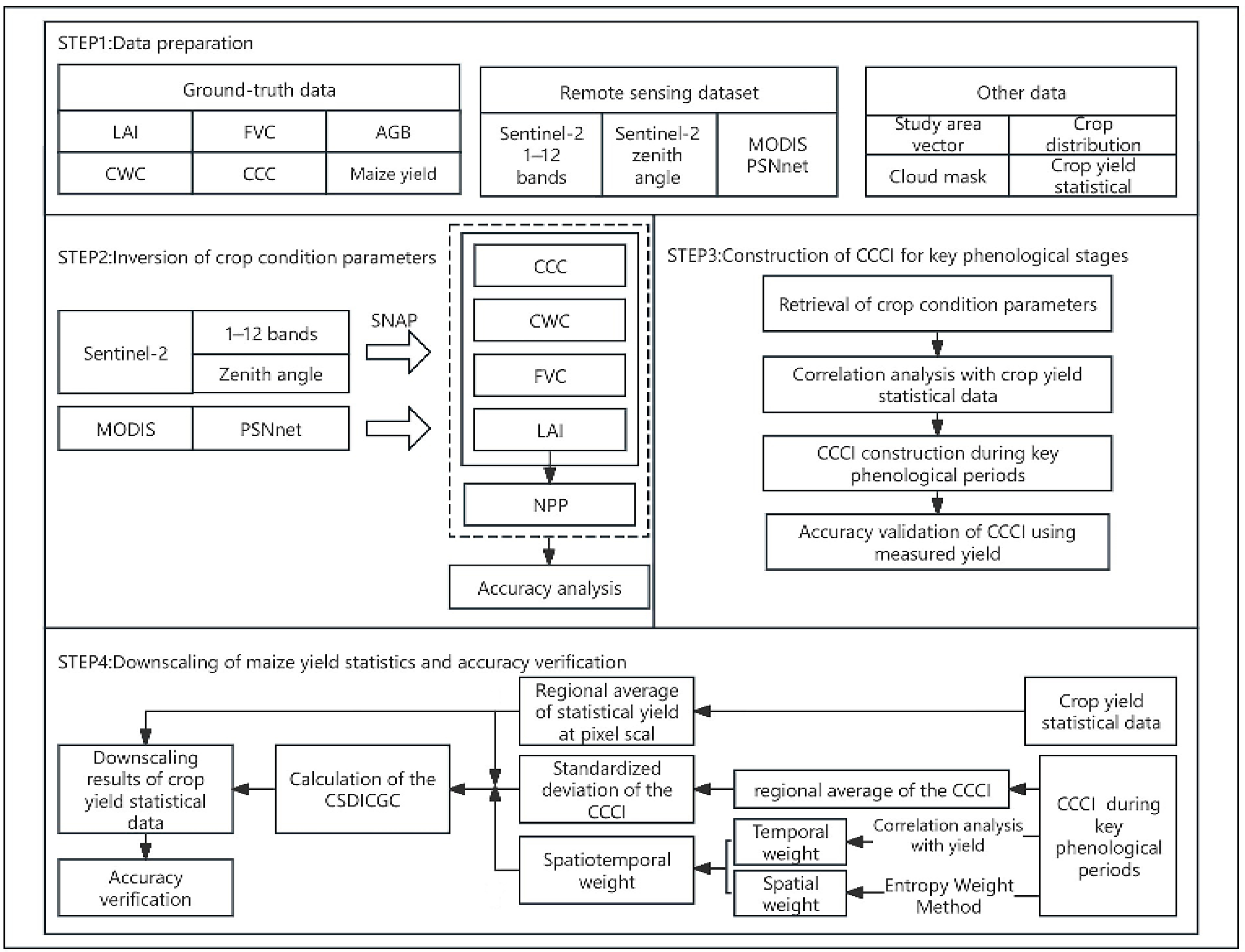
Supported by integrated observations from satellite–ground systems, this study utilized multisource remote sensing data during key phenological stages, ground-truth crop condition parameters, ground-truth maize yield, and regional statistical yield data. The CCCI was constructed using a normalized regression coefficient weighting method to characterize the crop growth status. Furthermore, the spatiotemporal dynamic weights of the index at each key phenological stage were determined by considering the temporal and spatial variations in crop growth. On this basis, a standardized deviation of pixels from the regional mean was introduced to develop the comprehensive spatial difference index of crop growth conditions (CSDICGC), providing a more accurate representation of pixel-level yield variation relative to the regional average. Finally, by combining the regional mean yield with the CSDICGC, the crop yield at the pixel scale within each administrative unit was estimated, thereby downscaling and spatializing the regional yield statistics. The overall technical framework of the study is illustrated in Figure 2.

3.2. Main Research Process

3.2.1. Comprehensive Crop Condition Index for Key Phenological Stages

In this study, four key phenological stages of maize growth—jointing, tasseling [42], milk maturity [43], and full maturity [44]—were selected because of their crucial influence on yield formation. Moreover, five major crop condition parameters—LAI, CWC, FVC, CCC, and NPP—were used. These parameters served as the main indicators reflecting crop growth status. The correlations between the crop condition parameters and yield during different phenological stages were taken as the basis for determining their weights, which were subsequently used to construct the CCCI for key phenological stages. The specific process is as follows:
(1)
Correlation Analysis between Crop Condition Parameters During Key Phenological Stages and Statistical Yield
A simple linear regression was established between each crop condition parameter and maize unit yield during the key phenological stages, with the regression coefficient used as the weighting reference. In this study, 53 ground-truth samples were collected to analyze the correlations between the crop condition parameters and unit yield for each key phenological stage.
Y = α i P i + b
In the formula, Y denotes the ground-truth unit yield (kg/ha), α i is the regression coefficient of the i-th crop condition parameter with the ground-truth yield, P i is the value of the i-th crop condition parameter in the key phenological stage, b is a constant, and a large α i indicates a strong effect of the crop condition parameter on the unit yield and thus a high assigned weight.
(2)
Construction of the CCCI for Key Phenological Stages Based on the Determination Method of Normalized Regression Coefficient Weights
In this study, the normalized regression coefficient weight determination method (NRCWDM) was employed to construct the CCCI for key phenological stages. Specifically, the regression coefficients obtained from the correlation analysis of each parameter with unit yield were first normalized. The normalized coefficients were then used as the weights of each parameter in the comprehensive index. Finally, the CCCI was computed for each key phenological stage using the weighted summation method:
P i k = P i k m i n P i k m a x P i k m i n P i k
F = i = 1 m α i / i = 1 m α i · P i
In the formula, P i k represents the normalized pixel value of the i-th crop condition parameter for the k-th pixel; m i n P i k and m a x P i k are the minimum and maximum values of the i-th parameter across all pixels, respectively; P i   d e n o t e s   t h e   n o r m a l i z e d   v a l u e   o f   t h e   i-th   p a r a m e t e r ;  F is the CCCI of the key phenological stage; and m is the total number of crop condition parameters, which in this study equals 5.

3.2.2. Calculation of the Comprehensive Spatial Difference Index of Crop Growth Conditions (CSDICGC)

(1)
Determination of the Temporal Weight Coefficient of the CCCI During Key Phenological Stages
A simple linear regression was established between the CCCI of each key phenological stage and the maize unit yield to determine the regression coefficient, which was used as the temporal weight reference of the index. In this study, 53 ground survey points were selected for the regression analysis of the crop condition indices and unit yield.
Y = β j F j + c
In the formula, Y represents the ground-truth maize yield (kg/ha); β j is the regression coefficient of the CCCI at the j-th phenological stage with the ground-truth yield, where a large β j indicates a great influence of the index on yield and therefore a high corresponding temporal weight; and c is a constant.
(2)
Calculation of the Difference Coefficient of the CCCI
To characterize the spatial heterogeneity of crop growth within the study area, the entropy weight method (EWM) was applied to calculate the difference coefficient of the CCCI, which reflects the degree of spatial variation in crop growth conditions. A large difference coefficient indicates high heterogeneity and a strong spatial differentiation ability of the index; conversely, a small coefficient indicates weak spatial representation. The difference coefficient was calculated as follows:
F j k = F j k k = 1 n F j k
σ j = 1 ln ( n ) k = 1 n F j k ln F j k
d j = 1 σ j
In the formulas, F j k is the proportion of the k-th pixel of the CCCI at the j-th phenological stage within the study area, n is the total number of crop pixels in the study area, σ j is the entropy of the j-th index, and d j is the difference coefficient of the index at the j-th phenological stage.
(3)
Calculation of the Spatiotemporal Weights of the CCCI
(a)
Temporal Weight Calculation
C j = β j / j = 1 t β j
In the formula, C j is the temporal weight of the index at the j-th phenological stage, and t is the total number of key phenological stages, where t = 4 in this study.
  •   (b)
    Calculation of the Spatial Weights of the CCCI
Spatial weights were calculated on the basis of the difference coefficient of the CCCI. A large difference coefficient indicates high heterogeneity, strong spatial differentiation ability, and thus a large weight. The equation is as follows:
D j = d j / j = 1 t d j
In the formula, D j is the spatial weight of the index at the j-th phenological stage.
  •   (c)
    Comprehensive Spatiotemporal Weight Calculation
E j = C j · D j
In the formula, E j is the normalized spatiotemporal weight of the index at the j-th phenological stage.
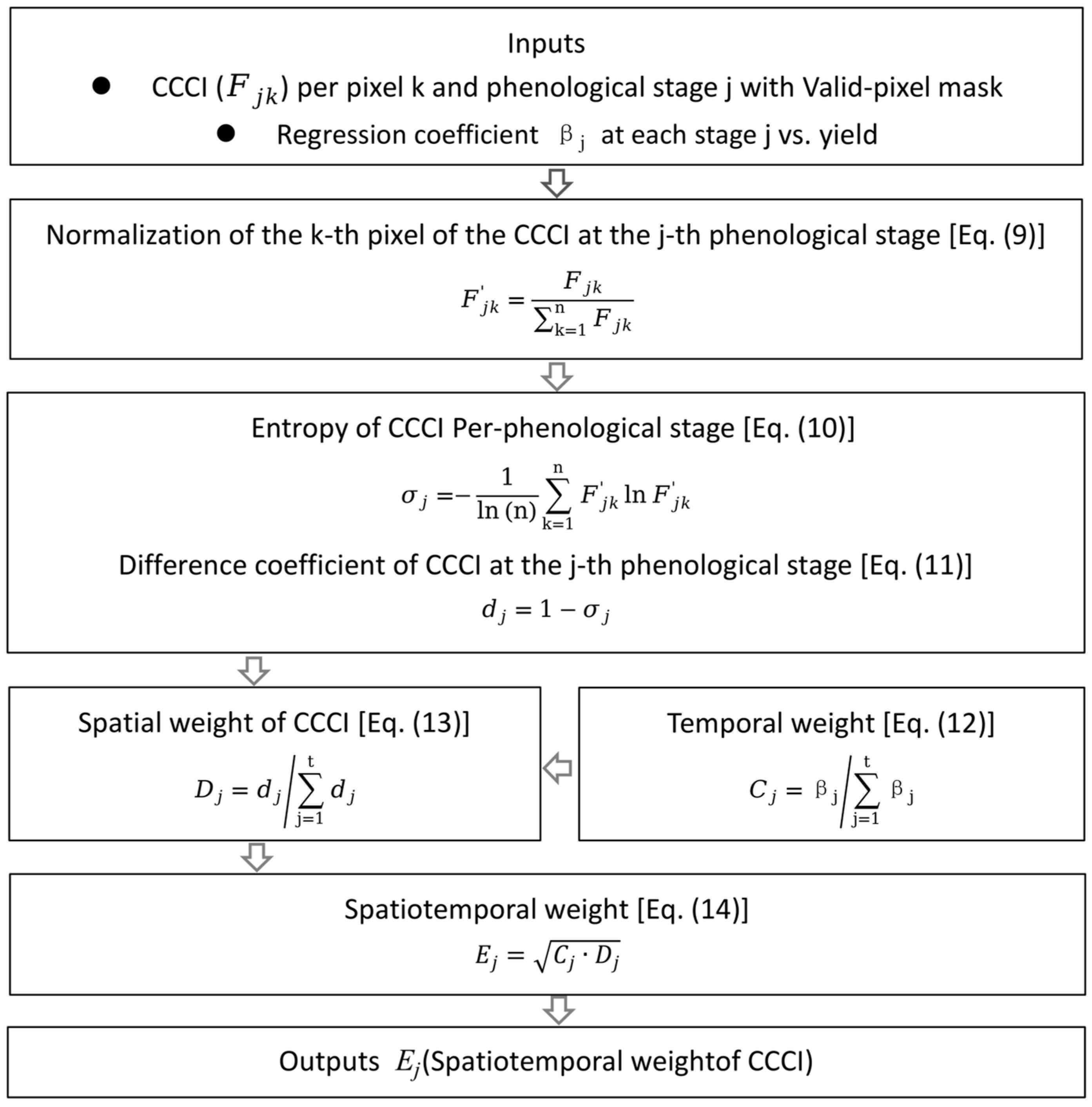
The concise algorithmic flow for calculating the difference coefficient of the CCCI (Equations (9)–(14)) is shown in Figure 3.
(4)
Calculation of the Comprehensive Spatial Difference Index of Crop Growth Conditions (CSDICGC)
Owing to the influence of environmental conditions, spatial heterogeneity exists in terms of crop growth within a region. To quantify this heterogeneity, the CSDICGC was proposed. At the pixel level, the regional mean of the comprehensive crop condition index was first calculated. Afterward, the standardized deviation of each pixel from the mean was combined with the normalized spatiotemporal weight to compute the comprehensive spatial difference index of the crop conditions.
(a)
Calculation of the Regional Average CCCI for Key Phenological Stages
F j ¯ = 1 n k = 1 n F j k
In the formula, F j ¯ is the regional mean of the CCCI at the j-th phenological stage (j ∈ 1, 2, …, 4), F j k is the value of the index at the k-th pixel, and n is the total number of pixels.
(b)
Standardized Deviation of the CCCI
G j k = F j k F j ¯ F j ¯
where F j k is the value of the index at the k-th pixel and G j k is the standardized deviation of the index at the j-th phenological stage for pixel k.
(c)
Calculation of the CSDICGC
H k = j = 1 t G j k · E j
In the formula, H k is the comprehensive spatial difference index of the crop growth condition for pixel k.

3.2.3. Downscaling of Maize Yield Statistics

The regional mean yield was multiplied by the CSDICGC to obtain the corresponding yield variation. Adding this variation to the regional mean yield enabled the transformation of maize yield statistics from the administrative unit scale to the pixel scale. Finally, ground survey yield data were used to validate the accuracy of the downscaled results.
Y k = Y ¯ + Y ¯ · H k
In this formula, Y ¯ denotes the statistical mean yield of the administrative unit in the study area (kg/ha), and Y k represents the yield of the k-th pixel (kg/ha).

3.2.4. Accuracy Verification

(1)
Accuracy Validation Based on Ground-Truth Data
In this study, ground survey sample points were used to validate the accuracy of the downscaled remote sensing inversion results for the crop condition parameters, CCCI, and crop yield. The CCCI was constructed from multiple crop condition parameters and lacks direct ground truth values. Therefore, its correlation with the measured yield was used as an indirect validation method [45]. A high correlation indicates a strong ability of the index to represent yield variations. The accuracy was evaluated using the coefficient of determination (R2), root mean square error (RMSE), normalized root mean square error (NRMSE), and mean relative error (MRE). For these metrics, R2 values close to 1 indicate high consistency, and small RMSE values indicate high accuracy. It is generally believed that simulation accuracy is considered excellent when the NRMSE and MRE are <10%, good when they are 10–20%, moderate when they are 20–30%, and poor when they are greater than 30% [46]. The validation samples in this study included 53 crop condition parameters, 53 CCCI values, and 22 yield per unit area results.
(2)
Regional Validation Crop Yield Statistics
In addition to pixel-scale validation, this study employed administrative unit yield statistics for regional-scale validation of the downscaled results. The regional mean yield ( R ) derived from the downscaled results was compared with the administrative unit statistical yield ( Y ¯ ) to determine the regional accuracy (w) within the study area.
R = 1 n k = 1 n Y k
w = 1 R Y ¯ Y ¯ · 100 %
where R represents the regional mean yield of the spatialized crop yield within the administrative unit of the study area; Y k is the yield of the k-th pixel (kg/ha) derived from the downscaled spatialization results; n denotes the total number of crop pixels within the study area; w refers to the regional accuracy of the spatialized crop yield results; and   Y ¯ is the statistical crop yield of the administrative unit in the study area (kg/ha).

4. Results and Analysis

On the basis of integrated sky–ground observation technologies, we applied a downscaling approach for crop yield statistics using multisource remote sensing data, ground-truth crop condition parameters, and regional statistical yield data. CCCI values were first constructed for key phenological stages, and their spatiotemporal weights were derived using a dynamic weighting method. Standardized deviations of the CCCI were then calculated at the pixel scale to obtain a growing-season spatial difference indicator through weighted summation. Finally, regional statistical yield data were integrated with this indicator to estimate pixel-scale maize yields, resulting in downscaled regional yield distributions.

4.1. Verification of the Inversion Results and Precision of the Main Growth Period Parameters

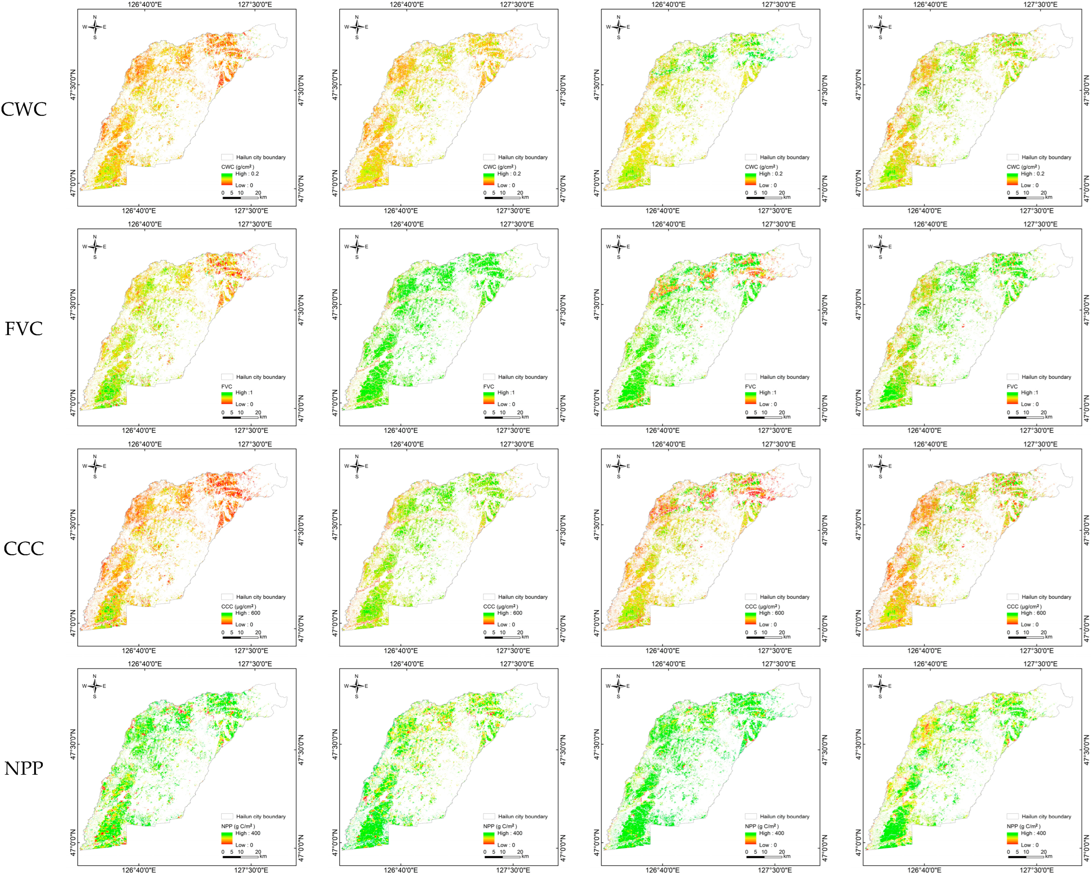
In maize yield predictions, crop condition parameters such as the LAI, CWC, FVC, CCC, and NPP are critical indicators of crop growth. These variables characterize physiological status and biomass accumulation from different perspectives and play an essential role in the spatialization of yield statistics. The accuracy of their remote sensing retrieval directly determines the reliability of the downscaling results. In this study, crop condition parameters at key phenological stages were retrieved using the BiophysicalO module in the SNAP model for Sentinel-2 imagery. The retrieved results included the LAI, CWC, FVC and CCC. In addition, NPP was calculated in combination with the 8-day composite MODIS data (Figure 4). These datasets provide a robust empirical basis for constructing CCCI and offer essential methodological support for the proposed downscaling framework for yield statistics.
As illustrated in Figure 4, the crop condition parameters clearly exhibited temporal dynamics across the main phenological stages. During the jointing stage, all the parameters remained relatively low, with an average LAI of 2.09 m2/m2 and an average CCC of 120.44 μg/cm2. The FVC was generally low (mean 0.60), except for a few high-value patches in the southern region, while more than 90% of the area recorded a CWC below 0.1 g/cm2. Low temperatures in June further suppressed NPP accumulation, with nearly 60% of the area showing 8-day totals below 237.31 g C/m2.
At the tasseling stage, crop growth peaks. The LAI, CCC, and FVC increased markedly, with most of the regions exceeding 6.5 m2/m2, 500 μg/cm2, and 0.9, respectively. Although CWC was slightly constrained by high temperatures in August, NPP accumulation was generally high, with a regional mean of 272.52 g C/m2.
During the milk stage, the LAI, CCC, and FVC decreased moderately compared with those during tasseling, but the CWC increased because of earlier rainfall, maintaining a relatively high mean value of 0.14 g/cm2. Moreover, sustained high temperatures in early to mid-August drove the NPP to its seasonal maximum, with nearly 90% of the area exceeding 228 g C/m2.
By the dough stage, senescence became evident. The LAI and CCC decreased sharply to 1.74 m2/m2 and 107.54 μg/cm2, respectively, while the FVC decreased to 0.44 and the CWC decreased substantially because of leaf dehydration. Similarly, as temperatures decreased in September, regional NPP accumulation decreased, with values below 239.8 g C/m2 across much of the central plain.
Overall, the remote sensing-derived crop condition parameters effectively captured both the temporal evolution and spatial heterogeneity of maize growth, providing a robust basis for yield spatialization at the pixel scale.
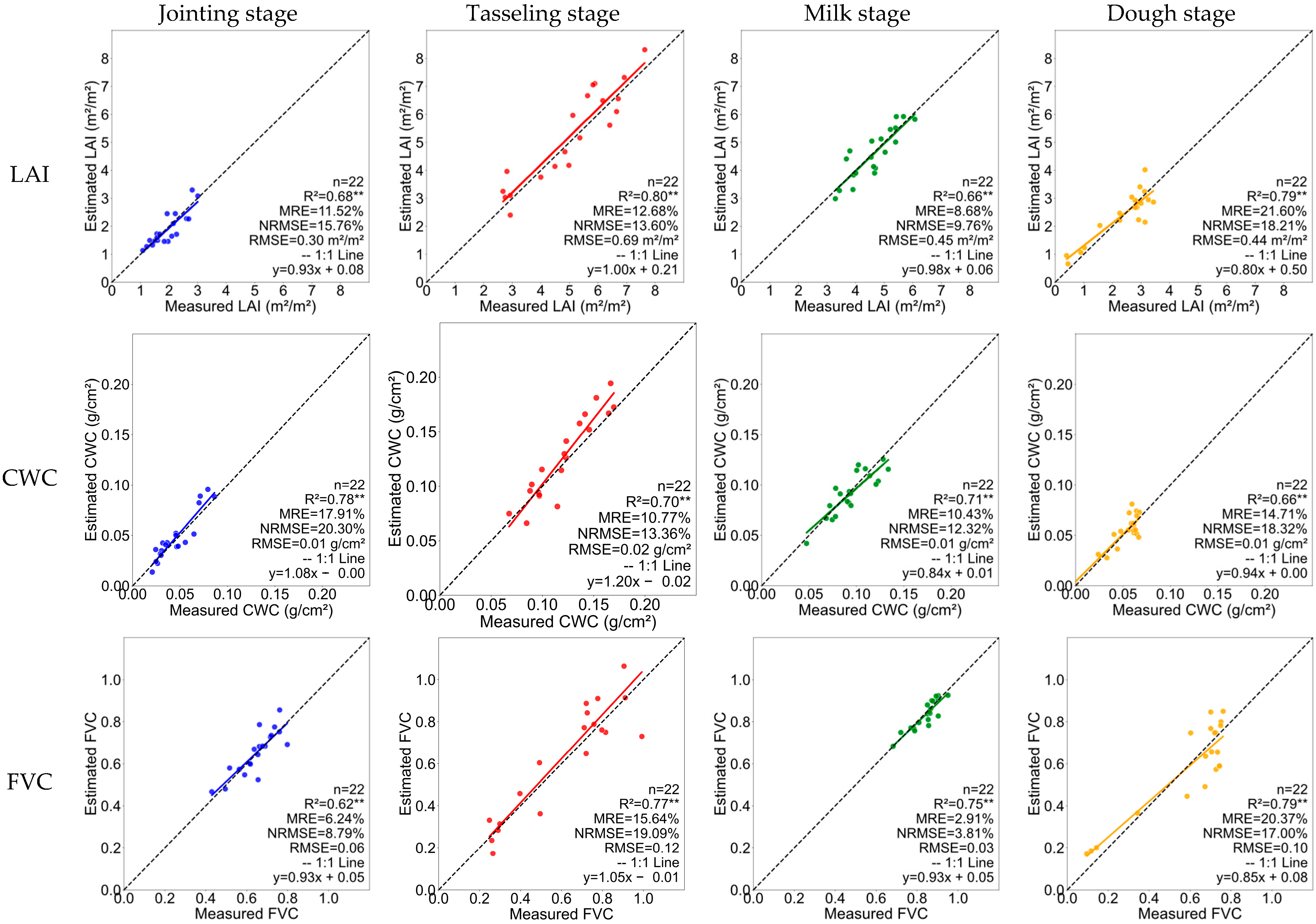
The results of the validation of the remote sensing retrievals against the in situ measurements of key crop condition parameters are shown in Figure 5. The inversion accuracy for the LAI yielded R2 values of 0.66–0.80, with RMSEs ranging from 0.30 to 0.69. For the CWC, the accuracy was slightly lower but still robust, with R2 values of 0.66–0.78 and RMSEs between 0.01 and 0.02 g/cm2. The retrieval of the maize CCC yielded R2 values of 0.68–0.79, with RMSEs ranging from 23.46 to 78.62 μg/cm2. For the FVC, the R2 values varied between 0.62 and 0.79, with RMSEs of 0.03–0.12, whereas for NPP, the R2 values ranged from 0.66–0.78, with RMSEs ranging from 14.87 to 41.24 g C/m2. In terms of the NRMSE, the five parameters ranged from 3.81–26.60%, with an average of 15.48%. These findings indicate that the retrievals of crop condition parameters demonstrated strong consistency with field observations and achieved sufficiently high accuracy to support subsequent yield downscaling applications.

4.2. Construction of the CCCI for Key Phenological Stages

Crop growth and yield formation are complex physiological and ecological processes influenced by multiple factors with pronounced temporal dynamics. Although remotely sensed crop condition parameters are correlated with yield, their relationships vary across growth stages. Reliance on a single parameter cannot fully characterize the spatial distribution of yield. In contrast, integrating multiple parameters from key phenological stages into a comprehensive index provides a more accurate representation of yield spatial patterns, thereby improving the downscaling accuracy of crop yield statistics.

4.2.1. Correlation Analysis Between Crop Condition Parameters in Key Phenological Periods and Crop Yield

To quantify the correlations between crop condition parameters and maize yield at different growth stages, four key stages—jointing, tasseling, milk, and dough—were selected, and linear regression models were established between the measured yield and major parameters, including the LAI, CWC, FVC, CCC, and NPP. The regression equations and accuracies are presented in Figure 6, and the corresponding correlation results are summarized in Figure 6.
The strength of the correlations varied across stages: during the jointing stage, the order was NPP > LAI > FVC > CCC > CWC; during tasseling, the order was LAI > NPP > CCC > FVC > CWC; during the milk stage, the order remained LAI > NPP > CCC > FVC > CWC; and during the dough stage, the order shifted to NPP > LAI > FVC > CCC > CWC. Overall, the LAI and NPP consistently exhibited the strongest correlations with maize yield, whereas the CWC showed the weakest correlations. When the different growth stages were compared, the overall correlation strength followed the order of tasseling > milk > dough > jointing, indicating that the crop condition parameters derived from the tasseling and milk stages were most strongly associated with yield.

4.2.2. Determination of Weights for Crop Condition Parameters in Key Phenological Periods

To construct a comprehensive index, the crop condition parameters at each stage were normalized and assigned weights on the basis of their regression coefficients with the observed yields; the detailed weight coefficients are presented in Table 4. Specifically, the weight of the LAI was lowest at the jointing stage (0.1976) and reached its highest value at the tasseling and dough stages (0.2183). The CWC exhibited its peak contribution during the milk stage (0.1894) before declining at the dough stage. The weight of the FVC was greatest at the jointing stage (0.2317) and gradually decreased to 0.1741 by the dough stage, reflecting its importance during early crop growth. The CCC reached its maximum at the tasseling stage (0.2110) and decreased to its lowest level at the dough stage (0.1479). In contrast, the NPP was highest during the dough stage (0.2882) and lowest during the tasseling stage (0.2108) and milk stage (0.2126), indicating that it progressively increased in contribution to yield formation during later growth stages.

4.2.3. Construction of the CCCI for Key Phenological Periods

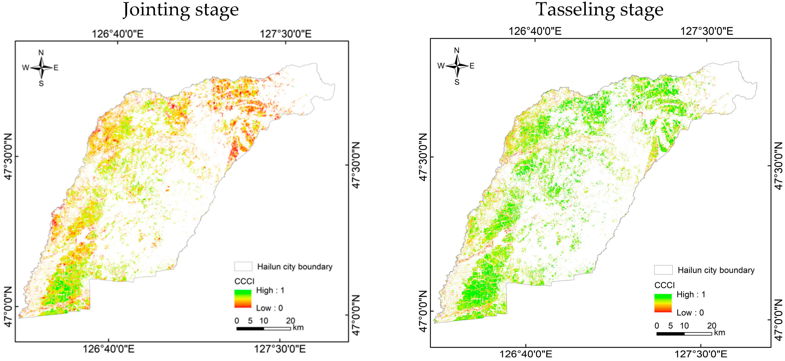
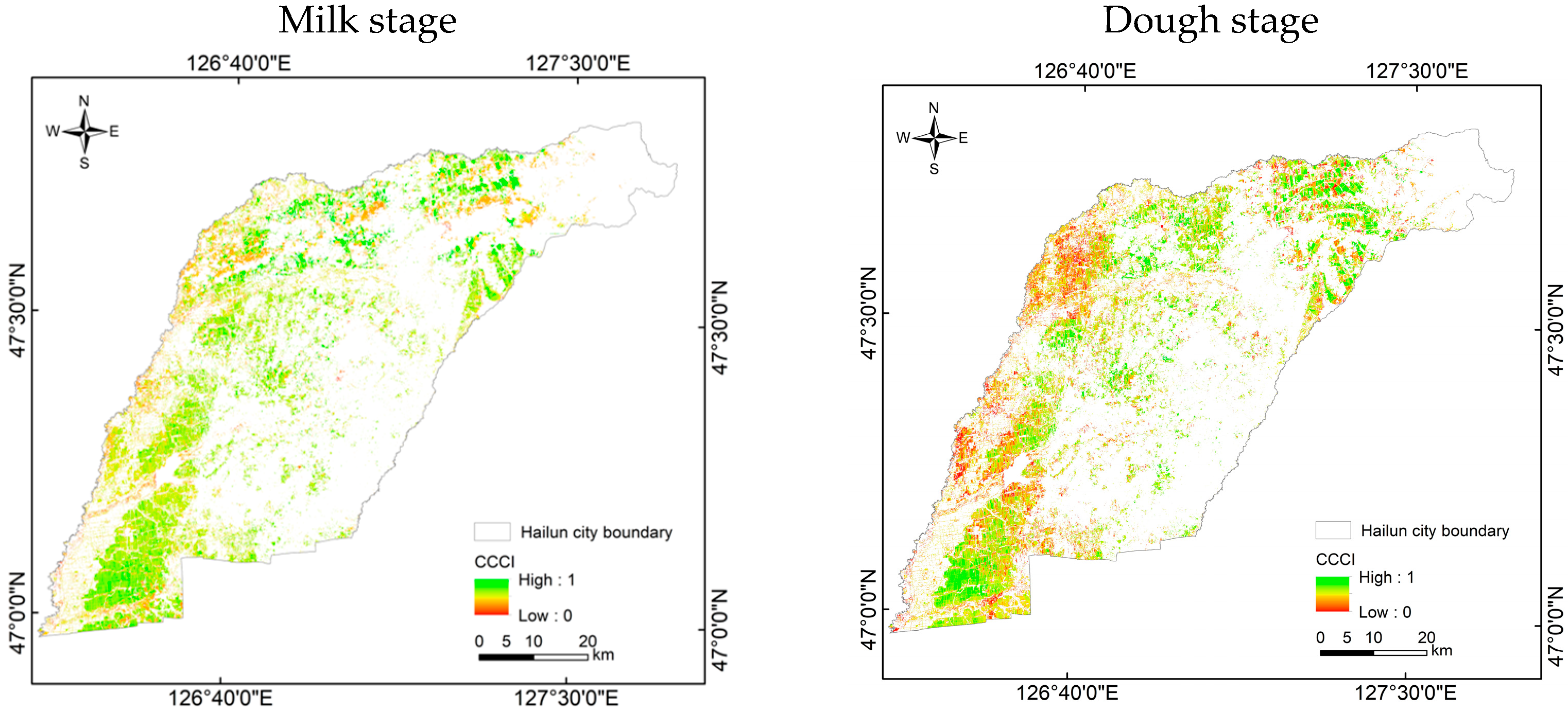
The weighted summation of the parameters yielded the CCCI (Figure 7). At the jointing stage, the overall values were relatively low, with a mean of 0.39, particularly in the northern regions, because of low temperatures in June, while the southern regions maintained relatively high temperatures. During the tasseling stage, more than 90% of the area reached peak values, benefitting from favorable temperature and precipitation conditions from July to early August. At the milk stage, the indices began to decline in some areas as a result of high temperatures and rainfall in late August. By the dough stage, the indices decreased rapidly in the central-western regions as leaf senescence and dehydration progressed, with certain areas remaining at relatively low levels.

4.2.4. Accuracy Verification of the CCCI for Key Phenological Stages

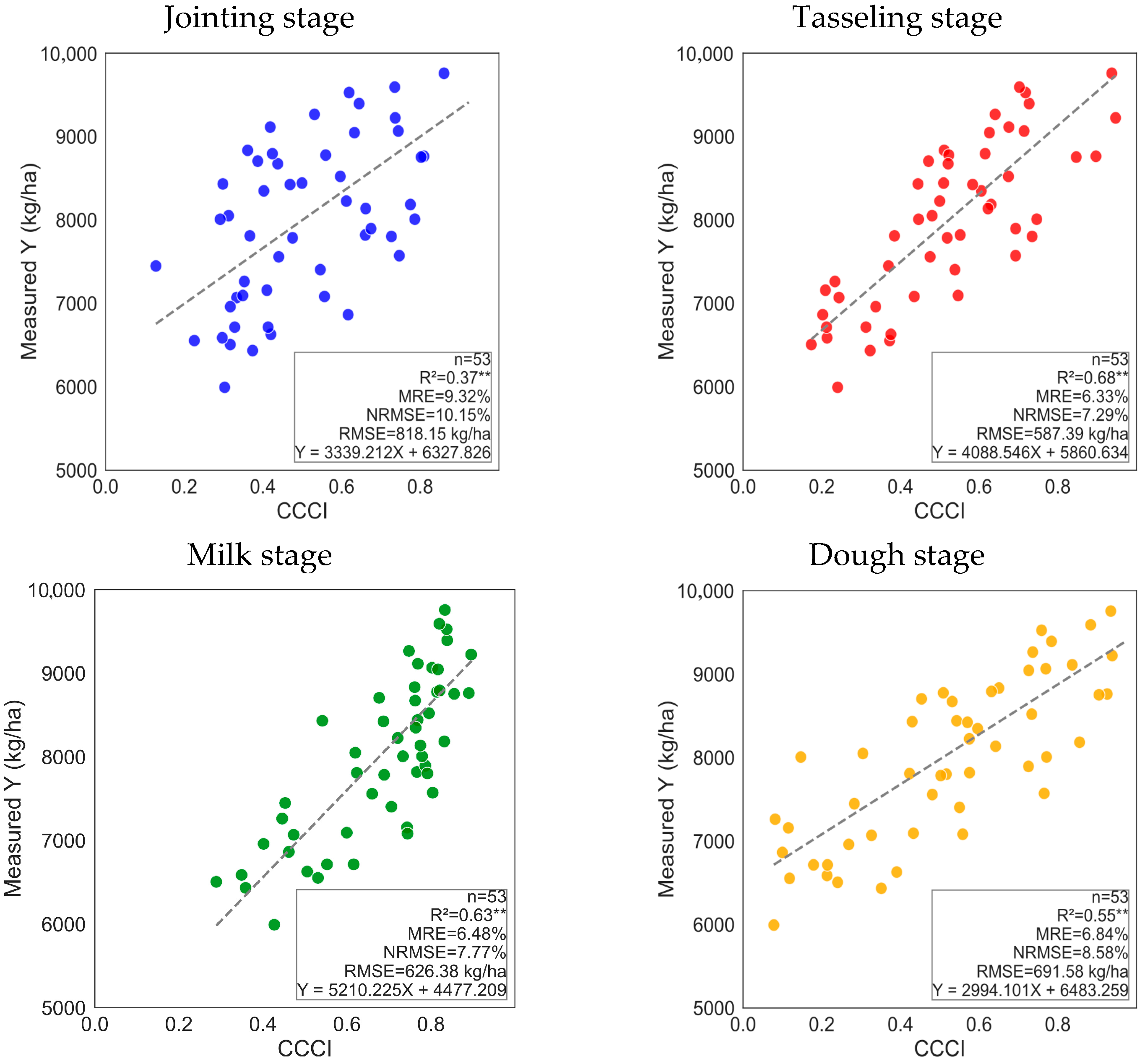
In this study, a simple linear regression model was developed to quantify the correlation between the CCCI at key phenological stages and ground-truth maize yield data. To evaluate the accuracy of the regression results and thereby characterize the reliability of the constructed indices, four statistical indicators were employed—the coefficient of determination (R2), root mean square error (RMSE), normalized root mean square error (NRMSE), and mean relative error (MRE). The correlation analysis results are summarized in Figure 8.
As shown in Figure 8, across the entire maize growing season, the CCCI of the key phenological stages exhibited highly significant correlations with yield, with the strength of the correlation following the order of tasseling stage > milk stage > dough stage > jointing stage. Specifically, the tasseling and milk stages showed the strongest correlations with ground-truth yield, with R2 values of 0.68 and 0.63, respectively; RMSE values of 587.39 kg/ha and 626.38 kg/ha, respectively; NRMSE values of 7.29% and 7.77%, respectively; and MRE values of 6.33% and 6.48%, respectively, whereas the jointing stage exhibited the weakest correlation. Compared with the correlations derived from single-crop condition parameters (e.g., the LAI, CWC, FVC, CCC, and NPP) at key stages (Figure 6), the advantages of the CCCI became evident. At the jointing stage, the single-parameter R2 values ranged from 0.13 to 0.33, whereas the CCCI was 0.37. During the tasseling stage, the single-parameter R2 values ranged from 0.41 to 0.66, whereas the CCCI reached 0.68. At the milk stage, the single-parameter R2 values ranged from 0.40 to 0.59, whereas the CCCI was 0.63. At the dough stage, the single-parameter R2 values ranged from 0.16 to 0.44, while the CCCI reached 0.55. As the CCCI integrates five crop condition parameters across four key phenological stages, it effectively mitigated the saturation effects observed for single parameters, while the inclusion of richer information further strengthened its correlation with yield. These findings demonstrate that, compared with the use of single-crop condition parameters, the use of the CCCI markedly enhances the explanatory power for spatial yield variation and provides a more robust representation of the dynamic yield patterns at key phenological stages, thereby offering a more reasonable and reliable framework for representing yield variation.

4.3. Calculations Based on the CSDICGC

The distribution of maize yield is strongly spatially heterogeneous because of environmental variability. To account for both temporal dynamics and spatial heterogeneity, this study employed temporal weights based on correlations with yield, spatial weights derived from the coefficient of variation, and standardized deviations to construct a comprehensive spatial difference index of the crop growth condition.

4.3.1. Calculation of the Time Weight for the CCCI During Key Phenological Periods

The CCCIs and yields were normalized, and the regression coefficients (Figure 8) were normalized to derive temporal weights (Table 5). The milk stage had the greatest temporal weight (0.34), highlighting its critical role in yield formation.

4.3.2. Calculation of Spatial Weights for the CCCI During Key Phenological Periods

Spatial heterogeneity was quantified by the coefficient of variation, with large values indicating strong heterogeneity and high spatial weight. The results (Table 6) revealed the highest spatial weight at tasseling (0.42) and the lowest at jointing (0.14), suggesting more uniform conditions during tasseling and greater variability at jointing.

4.3.3. Calculation of Spatiotemporal Dynamic Weight Coefficients for the CCCI During Key Phenological Periods

By integrating temporal and spatial weights (Table 5 and Table 6), the spatiotemporal dynamic weights were obtained (Table 7). The results revealed that the tasseling stage contributed the most to the yield distribution (0.34), followed by the milk (0.30) and dough (0.19) stages, whereas the jointing stage contributed the least (0.17), indicating that tasseling is the most influential stage in terms of driving spatial variability in maize yield.

4.3.4. Calculation of the CSDICGC

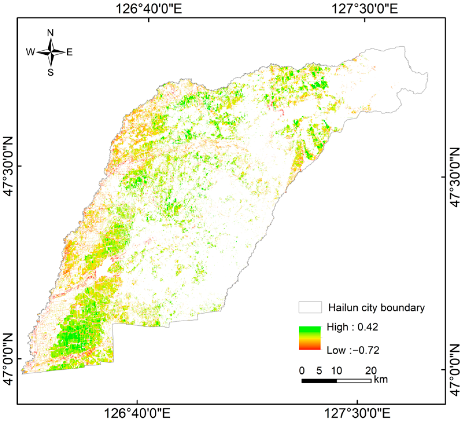
Using the spatiotemporal weights, standardized deviations were calculated to estimate the pixel-level deviations from the mean yield, resulting in the CSDICGC (Figure 9). The results revealed relatively small overall differences in 2023. This method further strengthened the correlation between the CSDICGC and the statistical yield. By comparing the number of pixels above and below the regional mean CSDICGC with the total maize pixels, we found that approximately 63% of the cropland area had CSDICGC values above the mean, indicating favorable crop growth conditions and a potential yield increase, whereas 37% of the area had values below the mean, suggesting a possible yield reduction.

4.4. Downscaling and Accuracy Analysis of Regional Maize Yield Statistical Data

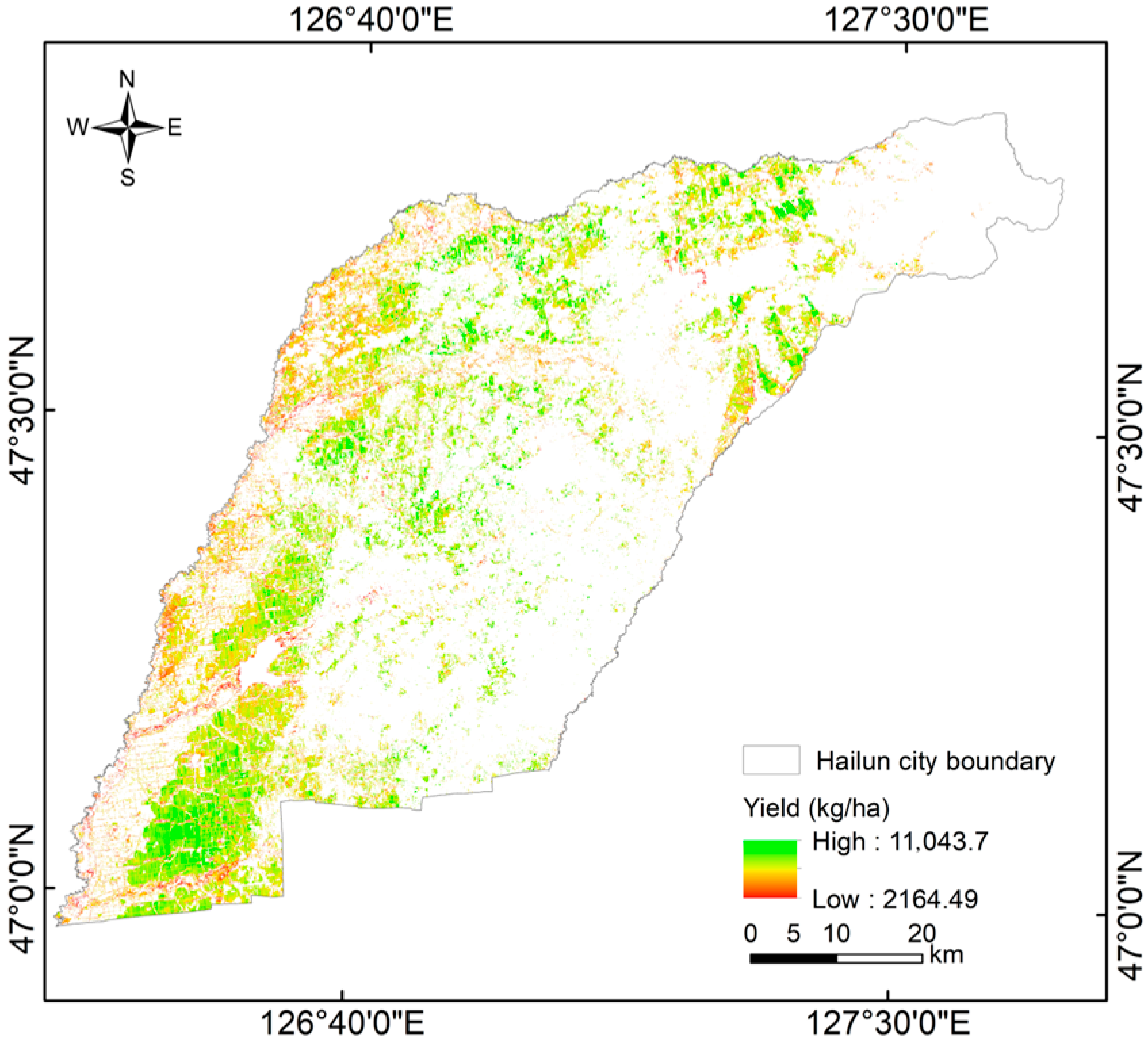
To achieve pixel-scale yield mapping, the regional mean yield was combined with the CSDICGC to estimate yield deviations, which were then added back to the mean (Figure 10). The results indicated that the maize yield distribution in Hailun city in 2023 was relatively uniform, with high yields observed in the southern region and slightly lower yields in the western region. Overall, 63% of the area exceeded the regional average yield, while 37% fell below. An accuracy assessment (Figure 11) further revealed that the regional average yield derived from downscaling was 7791 kg/ha, which was very close to the statistical yield of 7761 kg/ha, corresponding to a regional accuracy of 99.6%. Pixel-level validation with field data yielded an R2 of 0.82, an RMSE of 516.08 kg/ha, an NRMSE of 13.15%, and an MRE of 4.75%. A Moran’s I test was conducted using the 22 ground-truth points. The results showed that the Moran’s I value of the model residuals was –0.0385 (Z = 0.0930, p = 0.9238), indicating a random spatial distribution without significant spatial autocorrelation. These results confirm the effectiveness and feasibility of the proposed spatiotemporal weighting approach for downscaling maize yield statistics, enabling high-precision, large-scale yield mapping and providing a reliable data basis for yield estimation, forecasting, and precision agriculture applications, as well as for research on climate, resources, and disaster impacts.

5. Discussion

5.1. Limitations and Improvements of This Study

Because the study area in this research is relatively small and has fairly consistent hydrothermal conditions and agricultural management practices, the spatial distribution of maize phenological information within the region is relatively uniform. Therefore, the potential influence of phenological inconsistencies on the accuracy of the proposed spatiotemporal dynamic weighting–based method for downscaling maize yield statistics has not yet been considered. In future applications of this method at larger scales, it will be necessary to further account for spatial differences in crop phenology across broad regions. Zone partitioning based on phenological differences and research on the homogenization of phenological information will provide the basis for applying this method to large areas, which represents one of the key issues that needs to be addressed [47]. Building on this foundation, the expansion of the study area will require the incorporation of environmental, soil, and topographic factors to enable more refined regional partitioning. In future studies, the study area could thus be divided into relatively homogeneous subregions according to appropriate patterns, with representative ground-truth points selected for each subregion and weights adjusted accordingly, thereby enabling the model to better capture regional heterogeneity and improve its applicability across diverse areas [48].
In addition, when the integrated crop condition parameters were being constructed, this study employed the SNAP model of Sentinel data to quantitatively retrieve the major crop condition parameters. Although the accuracy of the parameters obtained through this method currently meets the requirements for yield downscaling in this study, the SNAP model was not specifically calibrated for the target crop. Therefore, in future large-scale applications, it will be necessary to retrieve crop-specific parameters, particularly through precise adjustment of the PROSAIL model parameters for different crop types, to account for crop-specific characteristics and further improve the accuracy of crop condition parameter estimations [49]. In addition, when using MODIS and Sentinel data to calculate other parameters (such as NPP), the default parameters provided in the MOD17 guide were used in this study. Although the calculation results met the accuracy requirements of this study, the uncertainty of the inversion results caused by the default parameters still needs to be further explored.
Moreover, in constructing the CCCI, this study considered only crop condition parameters and did not incorporate other relevant indicators, such as crop growth environment parameters or pest and disease information. Future research should aim to construct diversified composite indices that integrate multiple dimensions of indicators, thereby further enhancing the accuracy of the downscaling of crop yield statistics.

5.2. Innovations of This Study

(1)
A method for constructing the CCCI for key phenological periods based on the normalized regression coefficient weight determination method was outlined.
In existing research, when comprehensive crop growth indices are constructed using multiple crop condition parameters, weights among parameters are typically determined using methods such as the coefficient of variation, principal component analysis, the entropy weight method, gray relational analysis, as well as equal weighting or direct assignment. This study introduces a normalized regression coefficient weighting determination method to construct comprehensive agricultural condition indices specifically for key phenological periods. Unlike conventional studies that utilize single or multiple independent crop condition parameters for the downscaling of crop yield statistics, this research integrates multiple parameters to develop the CCCI, encompassing both crop growth structure and functional metrics. On the basis of the correlation analysis between the comprehensive index constructed in this study and the crop yield per unit area, this index can be used to characterize the spatial distribution of differences in crop yield effectively. Therefore, the proposed method for constructing the CCCI based on normalized regression coefficient weights provides reliable foundational data for the subsequent spatialization of crop yield statistical data in this research.
(2)
A method for expressing the spatial heterogeneity of crop growth status using temporally and spatially dynamic weights of the CCCI was proposed.
A review of the literature reveals that current research on crop yield spatialization has not utilized the CCCI to develop downscaling models for crop yield statistical data. In contrast, this study is the first to employ the CCCI based on key phenological periods for the spatialization of crop yield statistical data. In addition, in existing studies on the downscaling of crop statistical data, while some have considered the temporal characteristics of crops, the spatial heterogeneity of crop growth status within regions has not been addressed in the downscaling of crop yield statistics. This has hindered further improvements in the spatial accuracy of crop yield downscaling to some extent. In contrast, this study not only examined the correlations between crop condition parameters during key phenological periods and yield variations but also incorporated pixel-level heterogeneity in comprehensive crop condition parameters to explain regional yield differences. Therefore, the proposed method for expressing the spatial heterogeneity of crop growth status using temporally and spatially dynamic weights of the CCCI is important for enhancing the ability to simulate spatialized changes in crop yield at the pixel scale.
(3)
A downscaling method for crop yield statistical data based on the CSDICGC was proposed.
Existing studies have shown that conventional downscaling methods for crop yield statistics focus only on the linear relationship between crop vegetation indices and crop yield and directly apply this relationship at the pixel level without considering how each pixel deviates from the regional average. This approach somewhat compromises the downscaling accuracy of crop yield statistics at the pixel scale. Li et al. [21] developed the GCYS model, which achieved coefficients of determination (R2) of 0.72 and 0.76 at the regional scale. In contrast, the method proposed in this study was used the standardized deviation from the mean of the CCCI to characterize how pixel-scale yields deviate from the regional average yield level. This approach showed a high correlation with field-measured yield data at the pixel scale and achieved nearly 100% accuracy at the regional level. Moreover, it effectively avoided the saturation problem of single indices in direct methods and enabled the direct and reliable application of regional statistical yields at the pixel scale.
Additionally, machine learning methods could more flexibly simulate the distribution characteristics of crop yield. However, owing to sample size limitations, yield estimation models were usually first established at the regional scale and then applied them at the pixel scale. This process, however, often suffers from accuracy loss caused by scale transformation, making it necessary to use regional statistical yields as constraints to further optimize the spatialized results. In the research of Pei et al. [23], both XGBoost and RF achieved an average R2 of approximately 0.75, with RMSE values exceeding 1100 kg/ha. The county-level average NRMSE was 17.74%, all of which were lower than the accuracy obtained in this study (R2 = 0.82; RMSE = 516.08 kg/ha; NRMSE = 13.15%). The above results indicated that the accuracy of the proposed method in this study was superior to that of machine learning methods. At the same time, this research method to some extent avoided the shortcomings of machine learning methods that required further correction of the results.
Overall, this study pioneered a downscaling method for crop yield statistical data based on the CSDICGC. The proposed method was simple and efficient, held potential for large-scale applications, and effectively improved the pixel-level accuracy of downscaled crop yield statistics.

5.3. Application Prospects of This Study

The downscaling method for crop yield statistical data based on the standardized deviation from the mean of the CCCI in this study can generate large-scale, high-precision spatial distribution results of regional crop yield statistics. These results not only meet the urgent need for spatialized yield information in studies assessing the impacts of climate change, resource and environmental conditions, and natural disasters on food production systems but also facilitate the integration and comprehensive spatial analysis of yield statistics with other spatial datasets related to natural, geographic, and ecological factors. Furthermore, the spatialized yield results obtained through this method can support the expansion of training samples in pixel-scale crop yield prediction and estimation using machine learning or deep learning approaches, thereby providing an effective basis for large-scale crop yield estimation and prediction models as well as for accuracy verification. This addresses the common technical bottleneck in crop yield prediction research, where insufficient sample sizes hinder large-scale regional applications [50]. In addition, the application of this method to generate downscaled yield statistics is highly valuable for large-scale yield estimation and prediction in cases where no ground-based data are available. Moreover, the method ensures both regional- and pixel-scale accuracy in the downscaling results, which is of significant practical importance for meeting the demand for high-precision crop yield spatial distribution information in precision agriculture.

6. Conclusions

In this study, a downscaling method for maize yield statistical data based on the standardized deviation from the mean of the CCCI was proposed. By integrating multisource remote sensing data, ground-truth crop condition parameters, and regional statistical yields, the CCCI for key phenological stages was constructed. Combined with spatiotemporal dynamic weights to characterize the spatiotemporal heterogeneity of crop growth status, a comprehensive spatial difference index of crop growth conditions was obtained, which is highly important for the study of yield statistical data downscaling and spatial expression. Furthermore, this approach enabled the transformation of regional yield statistical data from the administrative unit scale to the pixel scale. The application of the method in Hailun city, Heilongjiang Province, demonstrated that the accuracy at the regional scale was close to 100%, whereas validation at the pixel scale revealed a strong correlation between the measured yields and spatialized yields (R2 = 0.82; RMSE = 516.08 kg/ha; NRMSE = 13.15%; MRE = 4.75%), confirming the rationality and feasibility of the method. The results not only provide a new approach for spatializing large-scale crop yield statistical data but also offer reliable data support for yield prediction, climate change impact assessment, and precision agriculture applications, highlighting the potential for broad regional application.

Author Contributions

Conceptualization, J.R.; methodology, J.R. and K.L.; software, K.L.; validation, K.L. and X.B.; formal analysis, K.L.; investigation, K.L., X.B. and H.Z.; resources, J.R.; data curation, K.L.; writing—original draft preparation, K.L.; writing—review and editing, all authors; visualization, K.L.; supervision, J.R.; project administration, J.R.; funding acquisition, J.R. All authors have read and agreed to the published version of the manuscript.

Funding

This work is supported by the National Key Research and Development Program of China (2023YFD1900101).

Data Availability Statement

The data presented in this study are available on request from the corresponding author. The data are not publicly available because of privacy restrictions.

Conflicts of Interest

The authors declare that they have no conflicts of interest.

References

  1. Soltani, A.; Galeshi, S.; Attarbashi, M.R.; Taheri, A.H. Comparison of two methods for estimating parameters of harvest index increase during seed growth. Field Crop. Res. 2004, 89, 369–378. [Google Scholar] [CrossRef]
  2. Deng, X.; Gibson, J.; Wang, P. Management of trade-offs between cultivated land conversions and land productivity in Shandong Province. J. Clean. Prod. 2017, 142, 767–774. [Google Scholar] [CrossRef]
  3. Khan, M.R.; de Bie, C.A.J.M.; van Keulen, H.; Smaling, E.M.A.; Real, R. Disaggregating and mapping crop statistics using hypertemporal remote sensing. Int. J. Appl. Earth Obs. Geoinf. 2010, 12, 36–46. [Google Scholar] [CrossRef]
  4. Hu, Y.; Wang, Q.; Liu, Y.; Li, J.; Ren, W. Index System and Transferring Methods to Build the National Society and Economy Grid Database. J. Geo-Inf. Sci. 2011, 13, 573–578. [Google Scholar] [CrossRef]
  5. Liu, Z.; Li, B. Spatial distribution of China grain output based on land use and population density. Trans. Chin. Soc. Agric. Eng. 2012, 28, 1–8. (In Chinese) [Google Scholar] [CrossRef]
  6. Fan, Y.; Shi, P.; Gu, Z.; Li, X.A. Method of Data Gridding from Administration Cell to Gridding Cell. Sci. Geogr. Sin. 2004, 24, 105–108. [Google Scholar] [CrossRef]
  7. Liu, X.H.; Kyriakidis, P.C.; Goodchild, M.F. Population-density estimation using regression and area-to-point residual kriging. Int. J. Geogr. Inf. Sci. 2008, 22, 431–447. [Google Scholar] [CrossRef]
  8. Yue, W.; Gao, J.; Yang, X. Estimation of Gross Domestic Product Using Multi-Sensor Remote Sensing Data: A Case Study in Zhejiang Province, East China. Remote Sens. 2014, 6, 7260–7275. [Google Scholar] [CrossRef]
  9. You, L.; Wood, S. Assessing the spatial distribution of crop areas using a cross-entropy method. Int. J. Appl. Earth Obs. Geoinf. 2005, 7, 310–323. [Google Scholar] [CrossRef]
  10. Monfreda, C.; Rarnankutty, N.; Foley, J.A. Farming the planet: Geographic distribution of crop areas, yields, physiological types and netprimary production in the year 2000. Glob. Biogeochem. Cycles 2008, 22, GB1022. [Google Scholar] [CrossRef]
  11. Potter, P.; Ramankutty, N.; Bennett, E.M.; Donner, S.D. Characterizing the Spatial Patterns of Global Fertilizer Application and Manure Production. Earth Interact. 2010, 14, 1–22. [Google Scholar] [CrossRef]
  12. Lobell, D.B.; Burke, M.B. On the use of statistical models to predict crop yield responses to climate change. Agric. For. Meteorol. 2010, 150, 1443–1452. [Google Scholar] [CrossRef]
  13. Zhu, X.; Shi, P.; Pan, Y. Development of a gridded dataset of annual irrigation water withdrawal in China. In Proceedings of the 2012 First International Conference on Agro-Geoinformatics (Agro-Geoinformatics), Shanghai, China, 2–4 August 2012; IEEE: New York, NY, USA, 2012; pp. 1–6. [Google Scholar] [CrossRef]
  14. Van Ittersum, M.K.; Cassman, K.G.; Grassini, P.; Wolf, J.; Tittonell, P.; Hochman, Z. Yield gap analysis with local to global relevance—A review. Field Crop. Res. 2013, 143, 4–17. [Google Scholar] [CrossRef]
  15. Woittiez, L.S.; van Wijk, M.T.; Slingerland, M.; van Noordwijk, M.; Giller, K.E. Yield gaps in oil palm: A quantitative review of contributing factors. Eur. J. Agron. 2017, 83, 57–77. [Google Scholar] [CrossRef]
  16. Iqbal, M.A.; Shen, Y.; Stricevic, R.; Pei, H.; Sun, H.; Amiri, E.; Penas, A.; del Rio, S. Evaluation of the FAO AquaCrop Model for Winter Wheat on the North China Plain under Deficit Irrigation from Field Experiment to Regional Yield Simulation. Agric. Water Manag. 2014, 135, 61–72. [Google Scholar] [CrossRef]
  17. Shi, S.; Chen, Y.; Li, Z. Spatial simulation of per unit area yield of maize by statistics based on regionalization and multiple regression analysis. J. Anhui Agric. Sci. 2011, 39, 3193–3195. (In Chinese) [Google Scholar]
  18. You, L.; Wood, S.; Wood-Sichra, U.; Wu, W. Generating global crop distribution maps: From census to grid. Agric. Syst. 2014, 127, 53–60. [Google Scholar] [CrossRef]
  19. You, L.; Wood, S. An Entropy Approach to Spatial Disaggregation of Agricultural Production. Agric. Syst. 2006, 90, 329–347. [Google Scholar] [CrossRef]
  20. Xiao, G.; Zhu, X.; Hou, C.; Liu, Y.; Xu, K. A Spatialization Method for Grain Yield Statistical Data: A Study on Winter Wheat of Shandong Province, China. Agron. J. 2019, 111, 1892–1903. [Google Scholar] [CrossRef]
  21. Li, J.; Zhang, H.; Xu, E. Spatialization of Actual Grain Crop Yield Coupled with Cultivation Systems and Multiple Factors: From Survey Data to Grid. Agronomy 2020, 10, 675. [Google Scholar] [CrossRef]
  22. Zhao, X.; Jin, T.; Dong, W.; Liu, M.; Liu, Q.; Liu, E. Spatialization of Spring Maize Yield Area in Northeast China Based on Multiple Linear Regression. Chin. J. Agrometeorol. 2023, 44, 1022–1031. (In Chinese) [Google Scholar] [CrossRef]
  23. Pei, J.i.e.; Zou, Y.; Liu, Y.; He, Y.; Tan, S.; Wang, T.; Huang, J. Downscaling Administrative-Level Crop Yield Statistics to 1 km Grids Using Multisource Remote Sensing Data and Ensemble Machine Learning. IEEE J. Sel. Top. Appl. Earth Obs. Remote Sens. 2024, 17, 14437–14453. [Google Scholar] [CrossRef]
  24. Ji, G.; Liao, S.; Yue, Y.; Hou, P.; Yang, X. Spatial distribution of grain yield based on different sample scales and partitioning schemes and its error correction. Trans. Chin. Soc. Agric. Eng. 2015, 31, 272–278. (In Chinese) [Google Scholar]
  25. Spaeth, S.C.; Randall, H.C.; Sinclair, T.R.; Vendeland, J.S. Stability of soybean harvest index. Agron. J. 1984, 76, 482–486. [Google Scholar] [CrossRef]
  26. Doraiswamy, P.C.; Hatfield, J.L.; Jackson, T.J.; Akhmedov, B.; Prueger, J.; Stern, A. Crop condition and yield simulations using Landsat and MODIS. Remote Sens. Environ. 2004, 92, 548–559. [Google Scholar] [CrossRef]
  27. Dempewolf, J.; Adusei, B.; Becker-Rehef, I.; Hansen, M.; Potapov, P.; Khan, A.; Barker, B. Wheat Yield Forecasting for Punjab Province from Vegetation Index Time Series and Historic Crop Statistics. Remote Sens. 2014, 6, 9653–9675. [Google Scholar] [CrossRef]
  28. Mkhabela, M.; Bullock, P.; Raj, S.; Wang, S.; Yang, Y. Crop yield forecasting on the Canadian Prairies using MODIS NDVI data. Agric. For. Meteorol. 2011, 151, 385–393. [Google Scholar] [CrossRef]
  29. Houborg, R.; Soegaard, H.; Boegh, E. Combining vegetation index and model inversion methods for the extraction of key vegetation biophysical parameters using Terra and Aqua MODIS reflectance data. Remote Sens. Environ. 2007, 106, 39–58. [Google Scholar]
  30. Gitelson, A.A. Wide dynamic range vegetation index for remote quantification of biophysical characteristics of vegetation. Plant Physiol. 2004, 161, 165–173. [Google Scholar] [CrossRef]
  31. Clerici, N.; Valbuena Calderón, C.A.; Posada, J.M. Fusion of Sentinel-1A and Sentinel-2A data for land cover mapping: A case study in the lower Magdalena region, Colombia. J. Maps 2017, 13, 718–726. [Google Scholar] [CrossRef]
  32. Hemmerling, J.; Pflugmacher, D.; Hostert, P. Mapping Temperate Forest Tree Species Using Dense Sentinel-2 Time Series. Remote Sens. Environ. 2021, 267, 112743. [Google Scholar] [CrossRef]
  33. Kandasamy, S.; Baret, F.; Verger, A.; Neveux, P.; Weiss, M. A comparison of methods for smoothing and gap filling time series of remote sensing observations—Application to MODIS LAI products. Biogeosciences 2013, 10, 4055–4071. [Google Scholar] [CrossRef]
  34. Chen, J.M.; Black, T.A. Defining leaf area index for non-flat leaves. Plant Cell Environ. 1992, 15, 421–429. [Google Scholar] [CrossRef]
  35. Kganyago, M.; Mhangara, P.; Alexandridis, T.; Laneve, G.; Ovakoglou, G.; Mashiyi, N. Validation of sentinel-2 leaf area index lai product derived from snap toolbox and its comparison with global lai products in an African semiarid agricultural landscape. Remote Sens. Lett. 2020, 11, 883–892. [Google Scholar] [CrossRef]
  36. Gitelson, A.A.; Viña, A.; Ciganda, V.; Rundquist, D.C.; Arkebauer, T.J. Remote estimation of canopy chlorophyll content in crops. Geophys. Res. Lett. 2005, 32, L08403. [Google Scholar] [CrossRef]
  37. Li, D.; Chen, J.M.; Zhang, X.; Yan, Y.; Zhu, J.; Zheng, H.; Zhou, K.; Yao, X.; Tian, Y.; Zhu, Y.; et al. Improved Estimation of Leaf Chlorophyll Content of Row Crops from Canopy Reflectance Spectra through Minimizing Canopy Structural Effects and Optimizing Off-Noon Observation Time. Remote Sens. Environ. 2020, 248, 111985. [Google Scholar] [CrossRef]
  38. Wang, B.; Jia, K.; Liang, S.; Xie, X.; Wei, X.; Zhao, X.; Yao, Y.; Zhang, X. Assessment of Sentinel-2 MSI spectral band reflectance for estimating fractional vegetation cover. Remote Sens. 2018, 10, 1927. [Google Scholar] [CrossRef]
  39. He, L.; Wang, R.; Mostovoy, G.; Liu, J.; Chen, J.; Shang, J.; Liu, J.; McNairn, H.; Powers, J. Crop Biomass Mapping Based on Ecosystem Modeling at Regional Scale Using High Resolution Sentinel-2 Data. Remote Sens. 2021, 13, 806. [Google Scholar] [CrossRef]
  40. Peng, D.; Huang, J.; Li, C.; Liu, L.; Huang, W.; Wang, F.; Yang, X. Modelling paddy rice yield using MODIS data. Agric. For. Meteorol. 2014, 184, 107–116. [Google Scholar] [CrossRef]
  41. Pearse, G.D.; Watt, M.S.; Morgenroth, J. Comparison of optical LAI measurements under diffuse and clear skies after correcting for scattered radiation. Agric. For. Meteorol. 2016, 221, 61–70. [Google Scholar] [CrossRef]
  42. Sun, Y.; He, Q.; Zhou, G.; Song, Y. Response of grain quality to plant growth dynamics in summer maize as influenced by sowing dates and weather factors. Ind. Crops Prod. 2025, 231, 121210. [Google Scholar] [CrossRef]
  43. Yang, B.; Zhu, W.; Rezaei, E.E.; Li, J.; Sun, Z.; Zhang, J. The Optimal Phenological Phase of Maize for Yield Prediction with High-Frequency UAV Remote Sensing. Remote Sens. 2022, 14, 1559. [Google Scholar] [CrossRef]
  44. Ren, Y.; Li, Q.; Du, X.; Zhang, Y.; Wang, H.; Shi, G.; Wei, M. Analysis of Corn Yield Prediction Potential at Various Growth Phases Using a Process-Based Model and Deep Learning. Plants 2023, 12, 446. [Google Scholar] [CrossRef]
  45. Yao, N.; Li, Y.; Liu, Q.Z.; Zhang, S.Y.; Chen, X.G.; Ji, Y.D.; Liu, F.G.; Pulatov, A.; Feng, P.Y. Response of Wheat and Maize Growth-Yields to Meteorological and Agricultural Droughts Based on Standardized Precipitation Evapotranspiration Indexes and Soil Moisture Deficit Indexes. Agric. Water Manag. 2022, 266, 107566. [Google Scholar] [CrossRef]
  46. Rinaldi, M.; Losavio, N.; Flagella, Z. Evaluation and application of the OILCROP–sun model for sunflower in southern Italy. Agric. Syst. 2003, 78, 17–30. [Google Scholar] [CrossRef]
  47. He, J.; Zhao, Y.; He, P.; Yu, M.; Zhu, Y.; Cao, W.; Zhang, X.; Tian, Y. Rice Yield Prediction Based on Simulation Zone Partitioning and Dual-Variable Hierarchical Assimilation. Remote Sens. 2025, 17, 386. [Google Scholar] [CrossRef]
  48. Guo, C.; Zhang, L.; Zhou, X.; Zhu, Y.; Cao, W.; Qiu, X.; Cheng, T.; Tian, Y. Integrating remote sensing information with crop model to monitor wheat growth and yield based on simulation zone partitioning. Precis. Agric. 2017, 19, 55–78. [Google Scholar] [CrossRef]
  49. Jiang, H.; Wei, X.; Chen, Z.; Zhu, M.; Yao, Y.; Zhang, X.; Jia, K. Influence of different soil reflectance schemes on the retrieval of vegetation LAI and FVC from PROSAIL in agriculture region. Comput. Electron. Agric. 2023, 212, 108165. [Google Scholar] [CrossRef]
  50. Ma, Y.; Zhang, Z.; Kang, Y.; Özdoğan, M. Corn yield prediction and uncertainty analysis based on remotely sensed variables using a Bayesian neural network approach. Remote Sens. Environ. 2021, 259, 112408. [Google Scholar] [CrossRef]
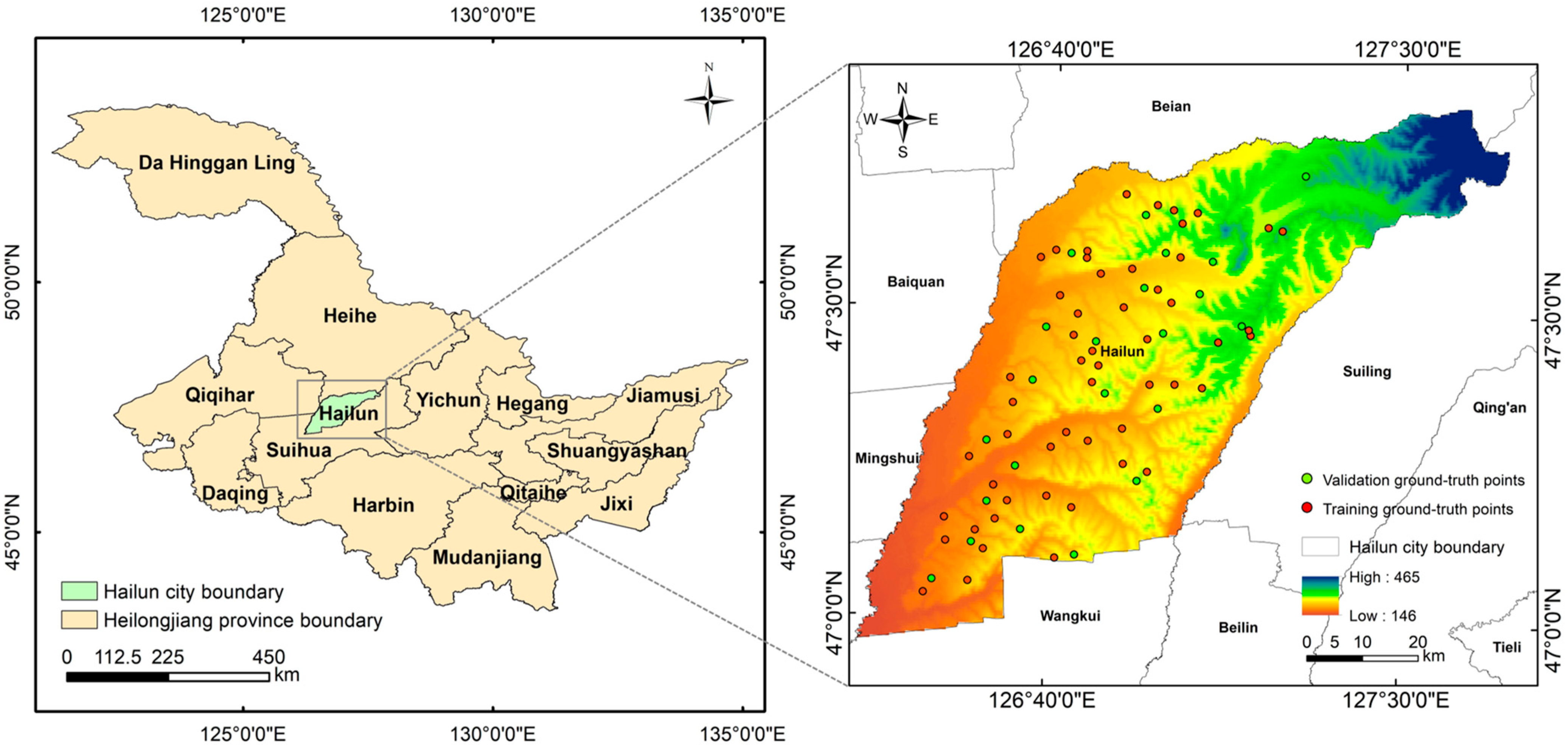
Figure 1. Location of the study area and distribution of ground-truth samples.
Remotesensing 17 03408 g001
Figure 2. Main technical framework employed in this study.
Remotesensing 17 03408 g002
Figure 3. Concise algorithmic flow of the comprehensive spatiotemporal weight calculation of the CCCI.
Remotesensing 17 03408 g003
Figure 4. Remote sensing inversion results of key crop condition parameters in the study area (2023).
Remotesensing 17 03408 g004aRemotesensing 17 03408 g004b
Figure 5. Verification results of the remote sensing inversion accuracy of key crop condition parameters in the study area (2023). Note: The units for the LAI are m2/m2, the units for CWC are g/cm2, FVC is dimensionless, the units for CCC are μg/cm2, and the units for NPP are g C/m2. In addition, ** indicates that the difference is extremely significant at the p < 0.01 level.
Remotesensing 17 03408 g005aRemotesensing 17 03408 g005b
Figure 6. Correlation between main crop condition parameters during key phenological periods and crop yield. Note: The units for LAI are m2/m2, the units for CWC are g/cm2, FVC is dimensionless, the units for CCC are μg/cm2, and the units for NPP are g C/m2. In addition, ** indicates that it reaches an extremely significant level at the p < 0.01 level.
Remotesensing 17 03408 g006aRemotesensing 17 03408 g006b
Figure 7. CCCI results for key phenological stages of maize (2023).
Remotesensing 17 03408 g007aRemotesensing 17 03408 g007b
Figure 8. Verification of the accuracy of the CCCI for key phenological stages of maize. Note: ** indicates that it reaches an extremely significant level at the p < 0.01 level.
Remotesensing 17 03408 g008
Figure 9. Spatial distribution of the CSDICGC (2023).
Remotesensing 17 03408 g009
Figure 10. Downscaling results of maize yield statistics in Hailun city (2023).
Remotesensing 17 03408 g010
Figure 11. Verification of the accuracy of maize yield statistics based on ground-truth yield data. Note: ** indicates that it reaches an extremely significant level at the p < 0.01 level.
Remotesensing 17 03408 g011
Table 1. Main phenological stages of maize in Hailun city.
NumberStagePhenological Stage Description
120 May–8 JuneSowing stage–Emergence stage
29 June–29 JuneEmergence stage–Three-leaf stage
330 June–19 JulyThree-leaf stage–Seven-leaf stage (Jointing stage)
420 July–1 AugustSeven-leaf stage (Jointing stage)–Tasseling stage
51 August–5 SeptemberTasseling stage–Grain filling (Milk stage)
65 September–30 SeptemberGrain filling (Milk stage)–Physiological maturity stage
Table 2. Remote sensing acquisition of crop condition parameters based on Sentinel-2 data.
NumberImage DateCrop Condition Parameter Names
120230702LAI, CCC, CWC, FVC
220230806LAI, CCC, CWC, FVC
320230828LAI, CCC, CWC, FVC
420230912LAI, CCC, CWC, FVC
Table 3. Ground survey data and main observation parameters.
NumberDate of Ground SurveyMain Ground Observation ParametersPhenological Period Description
120230702LAI, CCC, CWC, FVC, AGBJointing stage
220230806LAI, CCC, CWC, FVC, AGBTasseling stage
320230828LAI, CCC, CWC, FVC, AGBMilk stage
420230912LAI, CCC, CWC, FVC, AGBDough stage
520231002ground-truth maize yieldPhysiological maturity
Table 4. Weights of the main crop condition parameters in key phenological stages of maize.
Phenological Period DescriptionLAICWCFVCCCCNPP
Jointing stage0.19760.14120.23170.16810.2614
Tasseling stage0.21830.17570.18420.21100.2108
Milk stage0.20450.18940.20790.18560.2126
Dough stage0.21750.17230.17410.14790.2882
Table 5. Temporal weights of the CCCI for key maize phenological stages.
Weighting IndexJointing StageTasseling StageMilk StageDough Stage
Regression coefficient between CCCI and yield3339.2124088.5465210.2252994.101
Temporal weight0.210.260.340.19
Table 6. Spatial weights of the CCCI during key maize phenological stages.
Weighting IndexJointing StageTasseling StageMilk StageDough Stage
Coefficient of variation0.02570.07700.04400.0367
Spatial weight0.140.420.240.20
Table 7. Spatiotemporal dynamic weight coefficients of the CCCI for key phenological stages of maize.
Weighting IndexJointing StageTasseling StageMilk StageDough Stage
Spatiotemporal dynamic weight0.170.340.300.19
Disclaimer/Publisher’s Note: The statements, opinions and data contained in all publications are solely those of the individual author(s) and contributor(s) and not of MDPI and/or the editor(s). MDPI and/or the editor(s) disclaim responsibility for any injury to people or property resulting from any ideas, methods, instructions or products referred to in the content.