Highlights
What are the main findings?
- A new algorithm estimates bottom contamination probability from Sentinel-2 MSI reflectance, enabling the detection of optically shallow coastal waters.
- A near-infrared/blue spectral ratio algorithm improves chlorophyll-a retrieval in optically shallow lagoons compared to traditional algorithms.
What is the implication of the main finding?
- A full processing chain was developed and validated for high-resolution remote-sensing of water quality in optically complex coastal lagoons.
- The method provides a robust framework for the operational monitoring of anthropogenically impacted lagoon systems using Sentinel-2 MSI.
Abstract
Coastal lagoons are fragile and dynamic ecosystems that are particularly vulnerable to climate change and anthropogenic pressures such as urbanization and eutrophication. These vulnerabilities highlight the need for frequent and spatially extensive monitoring of water quality (WQ). While satellite remote sensing offers a valuable tool to support this effort, the optical complexity and shallow depths of lagoons pose major challenges for retrieving water column biogeochemical parameters such as chlorophyll-a ([chl-a]) and suspended particulate matter ([SPM]) concentrations. In this study, we develop and evaluate a robust satellite-based processing chain using Sentinel-2 MSI imagery over two French Mediterranean lagoon systems (Berre and Thau), supported by extensive in situ radiometric and biogeochemical datasets. Our approach includes the following: (i) a comparative assessment of six atmospheric correction (AC) processors, (ii) the development of an Optically Shallow Water Probability Algorithm (OSWPA), a new semi-empirical algorithm to estimate the probability of bottom contamination (BC), and (iii) the evaluation of several [chl-a] and [SPM] inversion algorithms. Results show that the Sen2Cor AC processor combined with a near-infrared similarity correction (NIR-SC) yields relative errors below 30% across all bands for retrieving remote-sensing reflectance Rrs(λ). OSWPA provides a spatially continuous and physically consistent alternative to binary BC masks. A new [chl-a] algorithm based on a near-infrared/blue Rrs ratio improves the retrieval accuracy while the 705 nm band appears to be the most suitable for retrieving [SPM] in optically shallow lagoons. This processing chain enables high-resolution WQ monitoring of two coastal lagoon systems and supports future large-scale assessments of ecological trends under increasing climate and anthropogenic stress.
1. Introduction
Coastal lagoons are paralic environments defined as shallow water bodies separated from the ocean by a geographical barrier and intermittently connected to it [1]. They are generally highly productive ecosystems, occupying around 13% of the global coastline [1,2,3]. Their marked physico-chemical and ecological gradients support exceptional biodiversity and sustain vital ecosystem services, including fisheries, aquaculture, tourism, and recreation [4,5,6,7,8].
However, these ecosystems are increasingly threatened by human-induced pressures and climate change. Due to their semi-enclosed nature and long water residence times, lagoons are particularly sensitive to nutrient enrichment, urban runoff and industrial discharges [2,6,9]. These stressors are further exacerbated by climate-driven events such as marine heatwaves, extreme precipitation, and extended windless periods, which can trigger major ecological crises [5,9]. A notable example is the 2018 summer anoxia crisis in several Mediterranean lagoons of southern France, which led to massive mortality of aquatic and shellfish species. In the Thau lagoon alone, nearly 4000 tons of oysters and mussels died, resulting in an estimated loss of 6 million euros for the shellfish industry [10].
Monitoring lagoon water quality (WQ) is essential to anticipate, mitigate, and manage such events. Within the framework of the European Union Water Framework Directive (WFD), member states are required to ensure the “good ecological and chemical status” of all surface water bodies, including lagoons. This assessment relies on several parameters, notably the concentrations of chlorophyll-a ([chl-a])—a proxy for phytoplankton biomass—and suspended particulate matter ([SPM]) [11,12,13]. Both parameters strongly affect water transparency, another key parameter under the WFD.
Traditionally, WQ indicators have been derived from in situ sampling and laboratory analyses, which offer high accuracy but suffer from limited spatial and temporal coverage. Point-based monitoring at fixed stations cannot fully capture the strong heterogeneity and rapid changes that characterize coastal lagoon systems [14,15]. In this context, satellite remote sensing has emerged as a valuable complementary tool. It enables regular, large-scale observations of water bodies and is increasingly used for WQ assessment under the WFD [16,17,18,19].
While ocean color missions were initially designed for open ocean monitoring, with typical spatial resolutions around 1 km [20,21,22], their applicability to coastal and inland waters is limited due to the small size and complexity of these environments [15,23]. To overcome this, high-resolution sensors such as Landsat-7 Enhanced Thematic Mapper Plus (ETM+), Landsat-8 Operational Land Imager (OLI) and Sentinel-2 Multispectral Imager (S2-MSI) have been widely used for coastal water studies [15], notably to retrieve and map WQ parameters including [chl-a] and [SPM] in coastal lagoons [17,24,25,26,27,28,29,30,31,32,33]. With its 10–20 m spatial resolution and frequent revisit time, S2-MSI is well-suited for mapping [chl-a] and [SPM], and other WQ indicators in coastal lagoons.
However, several challenges persist. Coastal lagoons are optically complex due to highly variable concentrations and compositions of optically active constituents such as phytoplankton, non-algal particles, and colored dissolved organic matter (CDOM). This complexity often undermines the applicability of standard bio-optical algorithms and increases reliance on site-specific algorithm calibration [28,34,35,36].
Moreover, the accuracy of WQ parameter retrievals depends heavily on the quality of the remote sensing reflectance (Rrs(λ)) derived from satellite radiometric measurements through atmospheric correction (AC). In lagoon environments, AC is particularly difficult due to adjacency effects, aerosol diversity, and frequent sunglint, all of which contaminate the top-of-atmosphere signal and affect the accuracy of the retrieved Rrs(λ) [15,29,34,37,38,39].
Additional complexity arises from the shallow nature of coastal lagoons, where bottom reflectance can contribute significantly to the water-leaving signal, particularly in clear waters. This bottom contamination (BC) can lead to biased retrievals of biogeochemical parameters within the water column if not properly accounted for [15,40,41]. A distinction is thus commonly made between optically shallow waters (OSWs), where BC is significant, and optically deep waters (ODWs), where it is negligible [42,43]. This classification depends on water depth, water transparency, wavelength and bottom albedo [44,45] and is a necessary step before applying inversion algorithms [40,46].
Considering all these elements, this study aims to develop a reliable high-resolution S2-MSI processing chain for monitoring [chl-a] and [SPM] in optically complex coastal lagoons. Our approach combines three key steps: (i) identifying the best AC processor to accurately retrieve Rrs(λ), (ii) developing a probabilistic algorithm to estimate BC and detect OSWs, and (iii) evaluating several inversion algorithms using both in situ measurements and satellite-derived Rrs(λ). The method is applied to two southern French lagoons, which exhibit contrasting morphologies and ecological conditions, providing an ideal testbed for assessing robustness and transferability of the approach. The analysis is supported by an extensive dataset combining S2-MSI imagery with in situ radiometric and biogeochemical measurements from multiple field campaigns.
2. Materials and Methods
2.1. Study Sites
The study focuses on two contrasted lagoon systems (Berre and Thau) along the French Mediterranean coast (Figure 1). According to the classification of [1], Berre is a “choked” lagoon, highly confined, with limited exchange with the sea through a single narrow inlet and strong riverine influence. In contrast, Thau is classified as a “restricted” lagoon, with two permanent connections to the sea allowing greater marine exchange and less fluvial influence. Although Bolmon (southern part of Figure 1A) is technically a sub-lagoon of Berre, it is considered separately in this study due to its shallow depth, persistent turbidity, and hypertrophic status.
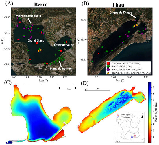
Figure 1.
S2-MSI images of the study sites: Berre (A) and Thau (B) lagoon systems, on the 25 March 2022 and 21 April 2024, respectively. The location of in situ stations used for bi-weekly (Thau, red squares), monthly (Berre, red squares) and casual (Thau, Berre and Bolmon, green and purple points) field sampling is shown, as well as the location of the station equipped with a HYPERNETS radiometric system (orange triangles H1 and H2, see Section 2.2). (C) Bathymetry maps of Berre (sources: SHOM, GIPREB, LITTO3D) and (D) Thau lagoons (source: Ifremer/Sextant).
- Berre lagoon
The Berre lagoon (Figure 1A) is located near Marseilles and is one of the largest coastal lagoons in Europe, covering ~155 km2 with an average depth of 6 m (max 9 m; Figure 1C). It connects to the Mediterranean Sea via the Caronte Canal and includes several sub-basins: the main “Grand Étang”, the “Étang de Vaïne” to the east, and the “Étang de Bolmon” to the south. Its natural watershed (~1600 km2) is drained by rivers such as the Arc, Touloubre, Durançole, and Cadière. Land use is heterogeneous: the Arc basin is largely forested, while the Touloubre catchment is more agricultural and urbanized, contributing diffuse nutrient inputs to the lagoon.
The lagoon is shaped by a Mediterranean climate and is strongly influenced by the Mistral, a dominant north–northwest wind that affects water circulation and mixing processes [47,48]. Since the mid-20th century, freshwater and nutrient inputs from the hydroelectric diversion canal have reinforced vertical stratification, reduced salinity, increased turbidity, and promoted recurrent eutrophication. These pressures have led to degraded ecological conditions, frequent hypoxic events, and the decline in benthic macrophyte populations [47,48].
- Thau lagoon
The Thau lagoon, near Montpellier, covers 68 km2 with an average depth of 4.5 m (max 10 m; Figure 1D). It exchanges water with the Mediterranean Sea through the Canals of Sète and the Grau de Pisses-Saumes. Circulation is wind-driven, with an average renewal time of 50 days. The lagoon is subject to a typical Mediterranean climate [9,10]. Its 269 km2 watershed combines natural areas, extensive vineyards, and urbanized zones. These heterogeneous catchments contribute to diffuse nitrogen (N) and phosphorus (P) inputs.
During the 20th century, increasing nutrient loads and rapid coastal development led to severe eutrophication and recurrent hypoxic crises (known as “malaïgues” in Occitan) that caused massive shellfish mortality [9,49]. Since the 1970s, improved wastewater treatment has reduced nutrient inputs, enabling a transition toward oligotrophic conditions. The lagoon is now classified as having “good ecological status” under the WFD. Shellfish farming remains a key activity, accounting for 10% of French oyster production [9], and continues to depend on strict WQ standards.
2.2. In-Situ Measurements
From 2018 to 2025, eight 2-day field campaigns were conducted: five in Berre (December 2018, November 2019, September 2021, October 2023, March 2024) and three in Thau (November 2022, June 2023, January 2025). During each campaign, radiometric measurements were performed onboard a boat, and surface water samples (1.5 L at 0.2 m depth) were collected for [chl-a] and [SPM] analyses.
In addition to these campaigns, long-term monitoring programs provide biogeochemical data. In Berre, [chl-a] and [SPM] have been measured monthly at 10 stations by the GIPREB (https://etangdeberre.org/, accessed on 16 April 2025). In Thau, [chl-a] is monitored every two weeks at two fixed stations under the REPHY (Réseau d’Observation et de Surveillance du Phytoplancton et des Phycotoxines) program coordinated by Ifremer [50]. All measurements follow standardized protocols, ensuring dataset consistency.
Since 2021, the autonomous HYPERNETS radiometer has been recording high-frequency above-water radiometric measurements at station H1 in Berre (Figure 1A), co-located with a GIPREB station. A second system was installed in 2025 at station H2 in Thau (Figure 1B), on a REPHY station. These deployments provide consistent radiometric and biogeochemical data for algorithm calibration and validation.
2.2.1. Laboratory [Chl-a] and [SPM] Analyses
[SPM] measurements followed the protocols detailed in [51,52]. Water samples were kept cool and dark, and filtered within 12 h. Between 150 and 1000 mL were filtered through pre-weighed, pre-combusted (450 °C) Whatman GF/F filters (0.7 µm, 25 mm, Whatman, Maidstone, UK). Filters were then stored at −80 °C in acid-washed, Milli-Q rinsed Petri dishes. Before weighing, they were dried for 24 h at 60 °C and weighed on a Mettler Toledo MX5 microscale (Mettler Toledo, Columbus, OH, USA) in a dehumidified room. [SPM] was computed as the difference between final and initial filter weights, divided by the filtered volume. When possible, triplicates were used to compute the mean and standard deviation values.
For [chl-a], 150 to 1500 mL of water were filtered on Whatman GF/F 25 mm filters, which were frozen at −80 °C until analysis. Pigments were analyzed via high-performance liquid chromatography at the SAPIGH platform (https://www.imev-mer.fr/web/service-analyse-de-pigment-par-hplc-sapigh/, accessed on 12 October 2025), following the method described in [53].
2.2.2. Radiometric Measurements and Data Processing
Radiometric data were collected using three TRIOS radiometers (350–950 nm, ~3.3 nm resolution, Trios Precision Engineering, Rastede, Germany) measuring above-water downwelling irradiance, Ed(λ) (W.m−2.nm−1), upwelling radiance, Lu(λ), and downwelling sky radiance Ls(λ) (W.m−2.sr−1.nm−1). Sensors were mounted following [54] to minimize sunglint: Lu and Ls were positioned at 40° and 140° from zenith, with a 90° azimuth offset from the Sun. Each station was measured for ~10 min with 10-s intervals. Rrs(λ) was computed as:
where , the air–water interface reflection coefficient, was fixed at 0.0256 [54,55,56]. The data processing protocol followed a combination of the methods described in [56,57]. The processing steps are as follows:
- A spectral interpolation to 1 nm was performed to standardize the wavelength grid across all TRIOS instruments.
- A threshold filter was applied to the Lu/Ed ratio in the 800–950 nm range (<0.025 sr−1) to remove scans with foam or object contamination.
- Consecutive Rrs(550 nm) values were required to deviate by less than 10% to filter out temporal variability or erroneous measurements.
- The NIR similarity correction (NIR-SC) described in [58] was applied using the 780 and 870 nm bands to correct for residual skylight or sunglint contamination.
- Negative corrected spectra were then excluded by applying the condition Rrs(400–800 nm) > 0.
- The remaining spectra were averaged to derive a representative spectrum for each station.
In addition to TRIOS data, autonomous radiometric measurements were acquired by the HYPERNETS system, which provides hyperspectral data (380–1020 nm, ~3 nm resolution) every 15 min during daylight hours. Water-leaving reflectance ( is processed using standardized protocols [57] and was downloaded from the Royal Belgian Institute of Natural Sciences servers. Processing steps (spectral alignment and interpolation, filtering, NIR-SC) are similar to those used for TRIOS. Although sensor specifications and processing methods differ slightly, a direct comparison of both systems at station H1 (Figure S1 in Supplementary Materials) confirms the consistency and reliability of the measurements. Further technical details are available in [57] and on the HYPERNETS websites (https://www.hypernets.eu; https://hypstar.eu, accessed on 18 April 2025).
2.3. Detection of Optically Shallow Waters (OSWs)
Accurately distinguishing between OSWs and ODWs is essential for reliable satellite retrievals of biogeochemical parameters such as [SPM] and [chl-a] [15,40,43,46]. Existing methods include empirical band ratios [41,59,60,61], semi-analytical model inversion and bottom detectability indexes [45,62,63,64] and machine learning approaches [46,61,65]. Each of these techniques presents limitations, including site-specific tuning, the need for hyperspectral data, sensitivity to Rrs(λ) uncertainties, and a lack of interpretability. Additionally, most rely on binary classification, which may introduce spatial artifacts in satellite-derived products. To address these issues, we developed OSWPA (Optically Shallow Water Probability Algorithm), a new approach that provides a continuous probability of BC based on robust spectral criteria.
2.3.1. Simulations of OSWs and ODWs
To develop and calibrate OSWPA, we simulated a total of 573 Rrs spectra using the forward implementation of the reference semi-analytical model in shallow waters developed by [45,62]. This model accounts for both water column inherent optical properties (IOPs) and bottom reflectance, making it suitable for simulating OSWs and ODWs. The model expresses the remote sensing reflectance just below the water surface rrs as a function of total absorption a, total backscattering bb, water depth H and bottom albedo :
where ; u = ; ; = 30° (subsurface solar zenith angle); = 10° (subsurface viewing angle from nadir). From Equation (2), Rrs is obtained as:
The IOPs were parameterized following the simplified formulation proposed by [62] using seven key inputs: (m−1) for phytoplankton absorption, (m−1) and spectral slope S for CDOM absorption, and spectral slope Sd for non-algal particles absorption, and (m−1) with slope γ for SPM backscattering. Pure water IOPs were taken from [66,67,68], and three bottom types were considered—sand, mud, and seagrass—using class-averaged spectra from [69]. The simulations were designed to represent diverse optical environments observed in the study sites (Berre, Thau, Bolmon):
- OSWs with high transparency and depths ranging from 1.5 to 7 m and three bottom types (hereafter referred as “sand”, “mud” and “seagrass”);
- ODWs with high transparency (hereafter referred as “deep”);
- Turbid waters (ODWs), characterized by high [SPM] and values (hereafter “turbid”);
- Phytoplankton bloom waters (ODWs), characterized by high [chl-a] and values (hereafter “blooms”).
Input parameters such as , , , , H, S, Sd and γ were selected to reflect realistic and contrasting conditions. The complete list of parameter values used for the simulations is provided in Supplementary Table S1. These synthetic spectra enabled the identification of robust spectral indicators of BC, forming the basis of OSWPA.
2.3.2. Optically Shallow Water Probability Algorithm (OSWPA)
OSWPA estimates the probability that a pixel or Rrs spectrum is contaminated by BC and thus represents an OSW, offering a continuous alternative to binary OSW/ODW classifications. It combines two spectral indicators identified from the simulated Rrs(λ) dataset (Section 2.3.1):
- The blue-to-green ratio RBG = Rrs(443)/Rrs(555), which is typically lower in OSWs due to the BC;
- The NIR-to-green ratio RNIRG = Rrs(705)/Rrs(555), which tends to increase in the presence of high phytoplankton biomass or turbidity.
Each spectral indicator is transformed into a probability score using a sigmoid function:
The coefficients were calibrated on the simulated hyperspectral Rrs database (Section 2.3.1; Table S1). The thresholds τBG = 0.6 and τNIRG = 0.1 were selected to best separate OSWs and ODWs according to the distribution of simulated ratios, while the steepness parameters kBG = 15 and kNIRG = 30 were set empirically to ensure smooth yet discriminant probability transitions. The final OSW probability POSWPA is computed as follows:
Equation (6) ensures that a high POSWPA is only reached when both indicators simultaneously suggest a significant BC.
2.4. Water Quality Retrieval Algorithms
The selected [chl-a] algorithms cover different model types and were chosen based on those reviewed in [70]. In addition, we propose a new algorithm based on the NIR/Blue Rrs ratio. This ratio was selected as it proved to be particularly robust in shallow waters, being less affected by BC. This choice is supported by our empirical results (Section 3.3.1), the results from [40], and simulations using the semi-analytical model of Lee [45]. Table 1 presents the full set of algorithms, including their equations, wavelengths, and references.

Table 1.
List of [chl-a] retrieval algorithms used in this study, including algorithm types, wavelengths used, references and mathematical expressions. Empirical coefficients a, b, c and d were calibrated using the method described in Section 2.5.
For [SPM], algorithms were selected based on the comparison made by [74] and the concentration range observed in the Berre, Thau and Bolmon lagoons (0–80 mg/L). Given this relatively narrow concentration range, we excluded switching-band models (e.g., [74,75]) and instead applied the Nechad [76] formulation at 560 and 705 nm. Table 2 summarizes the algorithms and their parameters.
Table 2.
List of [SPM] retrieval algorithms tested in this study, including algorithm types, wavelengths, references, and mathematical expressions. Empirical (a, b, c) and semi-empirical (Aₚ) coefficients were calibrated using the method described in Section 2.5, while Cₚ values were taken from the lookup table provided in [76].
In addition, we tested other algorithm families that were not included in the final comparison. A full inversion of the semi-analytical Lee model [45] was attempted but proved unreliable with S2-MSI due to its limited spectral resolution and residual AC uncertainties. Machine-learning approaches were also not retained, as our matchup dataset was too limited to train and validate robust models without risk of overfitting.
2.5. Calibration and Validation
The calibration and validation of [chl-a] and [SPM] algorithms relied on paired radiometric and in situ measurements (hereafter referred to as the BIO-CAL/VAL dataset: N = 100 for [chl-a], N = 89 for [SPM]). The BIO-CAL/VAL dataset was split into training (70%) and testing (30%) subsets using stratified sampling with the train_test_split function from scikit-learn, ensuring that the distributions of [chl-a], [SPM], and POSWPA were preserved. Stations for which the standard deviation of [SPM] triplicates exceeded 25% of the mean were excluded to ensure data quality. A detailed description of the full dataset distributions and of the resulting training and testing subsets is provided in Supplementary Table S2. Calibration was performed by least-squares minimization, adjusting model parameters to minimize S(p):
where yᵢ is the observed value, xᵢ the input (e.g., R or X), and p the set of model parameters to be adjusted. Validation used signed median bias (β) and median absolute percentage error (ε) as defined in [39], along with the coefficient of determination (R2) and the mean absolute error (MAE) for inter-study comparison.
2.6. Satellite Data, Atmospheric Corrections and Matchups
2.6.1. Sentinel-2 MSI Data
Sentinel-2A and 2B, respectively, operational since 2015 and 2017, provide 5-day revisit cycles at mid-latitudes, with an effective revisit of 2–3 days over the Berre Lagoon due to orbital overlap. The MSI sensor has 12 spectral bands covering the visible to short-wave infrared (SWIR) spectral regions, at 10 to 60 m spatial resolution. S2-MSI was selected for its high spatial/temporal resolution, 10-year consistency, and continuity via Sentinel-2C. Level-1C and Level-2A products were sourced from the CREODIAS platform (https://creodias.eu/, accessed on 25 February 2025).
2.6.2. Atmospheric Corrections
Accurate AC is critical for retrieving reliable Rrs in optically complex waters, where standard open-ocean algorithms often fail due to significant NIR water reflectance, aerosol heterogeneity, and adjacency effects [29,34,38]. Six AC algorithms were evaluated:
- Sen2Cor [79,80]: standard processor for S2-MSI Level-2A products. It estimates the aerosol optical thickness using the Dense Dark Vegetation method and performs corrections through look-up tables.
- ACOLITE [81,82]: applies the Dark Spectrum Fitting method, assuming zero reflectance in the SWIR bands over the darkest pixels. It is widely used for coastal waters due to its simplicity and efficiency [39,83].
- ACOLITE_glint: a modified ACOLITE version that includes an extra sunglint correction step, improving reflectance retrieval under sunglint-affected conditions.
- POLYMER [84]: this algorithm models atmospheric, sunglint, and water contributions through a polynomial spectral optimization. It performs well in glint-contaminated scenes and is compatible with S2-MSI.
- GRS [85]: estimates sunglint from SWIR bands, where water-leaving radiance is negligible, then extrapolates glint contribution to the visible spectrum using the bidirectional reflectance distribution function.
- C2RCC [86]: uses neural networks trained on large simulated datasets to retrieve Rrs, while accounting for sunglint and adjacency effects.
For Sen2Cor, ACOLITE, GRS and POLYMER, the NIR Similarity Correction (NIR-SC) described in [56,58] was applied to AC outputs to mitigate residual adjacency effects, sunglint, and skylight reflection. This correction is especially critical for Sen2Cor, as it lacks integrated skylight reflection correction. It assumes a nearly constant Rrs ratio in the NIR across low to moderate turbidity levels ([SPM] < 200 mg/L), a condition that holds true for turbidity ranges typically observed in coastal lagoons [87]. C2RCC did not require this step, as it already assumes zero reflectance in the NIR. Because the original wavelengths used by [56,58] (780 and 870 nm) are not available on S2-MSI, the correction was adapted using the closest available bands. The NIR-SC follows the equation:
where is the AC Rrs output at a given wavelength, .
2.6.3. Validation of Satellite-Derived Rrs(λ) and WQ Products
All satellite products (Rrs(λ), [chl-a], [SPM]) were resampled to 20 m resolution. For each station, a 3 × 3-pixel window was extracted, and a matchup was retained if ≥5 pixels were valid and the mean-to-standard deviation ratio exceeded 5, ensuring spatial homogeneity. A maximum time lag of 5 h was allowed between in situ sampling (typically between 09:00–13:00) and S2-MSI overpass. This process generated two validation datasets:
- Atmospheric Correction Validation (AC-VAL): 50 matchups with TRIOS and HYPERNETS Rrs data across Berre and Thau (Figure 1) were used to assess AC performance.
- Satellite-derived Water Quality Validation (SWQ-VAL): based on independent GIPREB and REPHY data. For [chl-a], 160 matchups were obtained (129 in Berre, 31 in Thau; 0.3–68 µg.L−1). No [chl-a] data was available for Bolmon. For [SPM], 129 matchups (0.6–19.8 mg.L−1) were collected in Berre only, as REPHY does not monitor [SPM] in Thau. SWQ-VAL was used to validate satellite-derived [chl-a] and [SPM].
Validation metrics included those from Section 2.5, as well as the log–log slope (S) [39], the root mean square error (RMSE), the linear regression slope and the intercept for AC validation. A detailed summary of the AC-VAL, BIO-CAL/VAL, and SWQ-VAL datasets—including campaign dates, sites, number of stations, measured parameters, and sensors used—is provided in Supplementary Table S3.
3. Results
3.1. Evaluation of Atmospheric Corrections Performances
Figure 2A shows the performance of S2-MSI AC processors, evaluated using ε, β, and S metrics based on comparisons with in situ Rrs(λ) from TRIOS (N = 29) and HYPERNETS (N = 21). Results are presented for each processor, with and without the application of NIR-SC (denoted “_sc”, see Section 2.6.2).
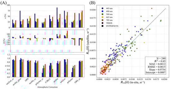
Figure 2.
Atmospheric correction (AC) performances of S2-MSI-derived Rrs in Berre and Thau lagoons: (A) ε, β, and S statistics associated with each AC, with and without applying the additional near-infrared similarity correction NIR-SC (denoted “_sc”). The statistics were computed based on observed differences between satellite-derived Rrs(λ) and in situ Rrs(λ) calculated from TRIOS (N = 29) and HYPERNETS (N = 21) measurements; (B) scatterplot and additional statistics concerning the Sen2Cor_sc AC.
Sen2Cor with NIR-SC (Sen2Cor_sc) performed best overall, followed by ACOLITE_glint and GRS. These three processors include a sunglint correction step, which proved essential in the sunglint-prone conditions of our study sites. The NIR-SC systematically improved the results, except for GRS, and was particularly beneficial for Sen2Cor, reducing both relative error and bias by half. Notably, Sen2Cor is the only processor that does not inherently correct for skylight reflection. Sen2Cor_sc reached relative errors below 30% for most bands (e.g., ε = 34% at 443 nm, 19% at 490 nm, 14% at 560 nm, 20% at 665 nm, 31% at 705 nm) with moderate biases (β = +28% at 443 nm, +23% at 490 nm, 0% at 560 nm, +10% at 665 nm, −10% at 705 nm). The log–log slope S remained close to 1 across all bands, indicating good sensitivity to Rrs magnitude. Figure 2B further confirms Sen2Cor_sc’s accuracy (R2 = 0.87, MAE = 0.0012 sr−1, RMSE = 0.0015 sr−1, regression slope = 0.975, near-zero intercept). The best agreement with in situ data was found for the 560 nm band, while higher errors and biases occurred at 443 and 705 nm. Bands beyond 705 nm were excluded due to low signal-to-noise and limited relevance for subsequent analyses.
3.2. Optically Shallow Water Probability Algorithm (OSWPA)
Figure 3 presents simulated Rrs spectra for OSWs and ODWs (Figure 3A) and the two-dimensional feature space used by OSWPA (Figure 3B). Spectra (normalized at 555 nm) were generated using the semi-analytical model of [45] across diverse conditions described in Section 2.3.1.
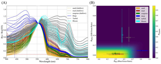
Figure 3.
Simulated Rrs spectra and Optically Shallow Water Probability Algorithm (OSWPA) feature space. (A) Normalized Rrs spectra (at 555 nm) simulated from the Lee model [43]; dotted lines: OSWs (sand, mud, seagrass), solid lines: ODWs (Deep, Turbid and Bloom, see Section 2.3.1 and Table S1). Dashed vertical lines at 443 nm and 705 nm indicate the wavelengths while horizontal lines represent the thresholds used in OSWPA. (B) OSWPA feature space based on RBG and RNIRG ratios. Background shows modeled POSWPA; boxplots represent ratio distributions by water type.
Two spectral windows in the blue (443 nm) and in the NIR (705 nm) clearly separate OSWs from ODWs (highlighted by vertical dashed blue and red lines). The blue-to-green Rrs ratio (RBG = Rrs(443)/Rrs(555)) effectively discriminates OSWs from ODWs, though overlaps occur with bloom and turbid waters. The NIR/green Rrs ratio (RNIRG = Rrs(705)/Rrs(555)) helps to further isolate OSWs from these overlapping spectra. From these observations, two empirical thresholds were derived: τBG = 0.6 and τNIRG = 0.1, represented by horizontal dashed lines on Figure 3B.
Figure 3B displays the OSWPA feature space defined by the RBG and RNIRG ratios. The color scale shows the modeled BC probability (POSWPA), and boxplots illustrate spectral ratio distributions for each category. OSWs cluster in the lower-left quadrant (RBG < 0.6, RNIRG < 0.1). “Deep” ODWs show higher RBG (>0.65) and lower and stable RNIRG (~0.12). “Bloom” and “turbid” ODWs span broader RNIRG ranges (0.15–0.80), reflecting wide ranges of [chl-a] and [SPM]. As [chl-a] or [SPM] decreases, RNIRG tends to approach OSWs values. Within OSWs, RNIRG remains low and stable (0.01–0.05), indicating a low sensitivity of this ratio to bottom type or water depth. On the contrary, when water depth increases, RBG gradually converges toward a “deep” RBG signature due to reduced BC (see, for example, the right extremity of the “mud” RBG distribution in Figure 3B).
Figure 4 compares RGB composites and POSWPA maps derived from S2-MSI imagery for selected dates in the Berre (A) and Thau (B) lagoons. It illustrates the algorithm’s response across a range of optical and biogeochemical conditions, including clear waters, turbid plumes, and phytoplankton blooms.
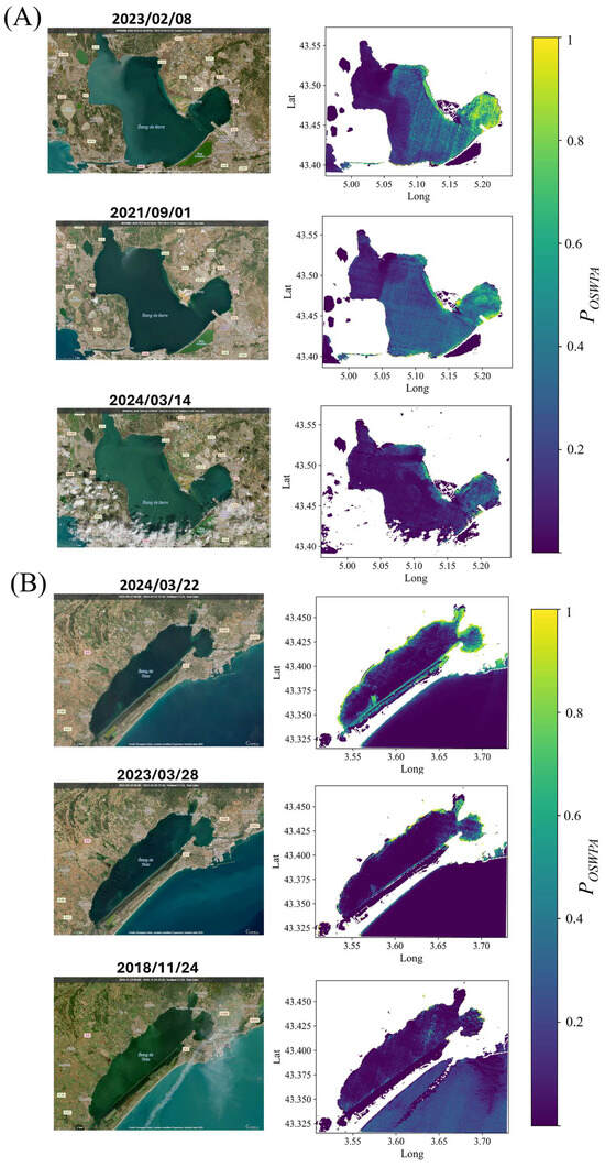
Figure 4.
Examples of S2-MSI RGB composites and POSWPA maps for Berre (A) and Thau (B) lagoons computed by OSWPA. The represented dates were selected to illustrate different optical and biogeochemical conditions.
In the Berre lagoon (Figure 4A), OSWPA consistently highlights shallow sandy zones with strong BC, such as the central shoal and the “Étang de Vaïne” (see Figure 1A,C). On 8 February 2023, under clear water conditions, POSWPA exceeds 0.8 in these areas, while the adjacent turbid discharge plume from the hydroelectric canal is correctly excluded. This indicates the algorithm’s ability to distinguish BC from turbidity. Similar results are observed on 1 September 2021, with slightly lower POSWPA values, likely due to seasonal reductions in water clarity. On 14 March 2024, under mesotrophic conditions confirmed by in situ data ([chl-a] between 5 and 12 µg/L), OSWPA values remain high in shallow sandy zones but with reduced spatial extent, reflecting lower water transparency. Importantly, the Bolmon lagoon (southeast of the Berre lagoon, see Figure 1A), despite its shallow depth (<2 m), consistently shows null POSWPA values across all dates. This aligns with its persistent high turbidity, driven by elevated phytoplankton concentrations ([chl-a] > 80 µg/L) year-round. This case illustrates OSWPA’s ability to distinguish optically shallow waters from productive turbid waters, even in areas where depth alone might suggest strong BC.
In the Thau lagoon (Figure 4B), POSWPA patterns closely match known bathymetric features and optical properties (see Figure 1D). On 22 March 2024, clear water conditions allow strong BC to be detected along shallow sandy fringes, including the “crique de l’Angle” and a southwestern shoal. However, the shallowest end of the “crique de l’Angle” (<1 m depth) shows no BC (POSWPA ≈ 0), which may suggest that the algorithm does not capture extremely shallow waters where NIR reflectance can be affected by the bottom substrate. Central deeper areas with muddy substrate show low POSWPA values, as expected. On 28 March 2023, moderate water turbidity due to sediment resuspension slightly lowers POSWPA values. During a bloom on 24 November 2018, the entire lagoon shows near-zero values, except for a few residual shallow patches, confirming the algorithm’s ability to avoid confusing turbid waters with BC.
Additional validation results are provided in the Supplementary Materials, including the application of OSWPA on a third site (Bizerte lagoon, Tunisia, Figure S2), a comparison of the method with the deep neural networks (DNNs) approach of [46] (Figure S3), and a quantitative relationship between POSWPA and water depths in Berre on an S2-MSI image (Figure S4).
3.3. Water Quality Retrieval Algorithms: Calibration and Validation
3.3.1. [Chl-a]
Figure 5 shows log–log scatterplots between in situ [chl-a] and various Rrs band ratios, with each point representing a BIO-CAL/VAL station (Figure 1A,B). Marker shapes distinguish the lagoons (Berre, Thau, Bolmon), while the color scale indicates the POSWPA value, reflecting the likelihood of BC estimated by OSWPA.
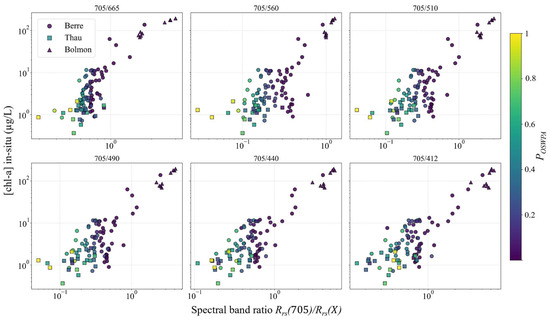
Figure 5.
Log-to-log scatterplots between in situ [chl-a] and spectral band ratio Rrs(705)/Rrs(X), with X = 665, 560, 510, 490, 440 and 412 nm based on the BIO-CAL/VAL dataset. The color-scale indicates POSWPA, the likelihood of bottom contamination (BC) computed by OSWPA (see Section 2.3.2).
Clear differences emerge across the spectral ratios tested for [chl-a] retrieval, especially when accounting for BC using POSWPA. The Rrs(705)/Rrs(665) ratio, widely used in turbid and productive coastal or inland waters, shows a curved relationship with considerable scatter for stations highly contaminated by the sea bottom (POSWPA > 0.5). This increased variability likely results from the overestimation of Rrs(665), which is sensitive to BC in shallow areas, leading to an artificially low ratio and deviation from the main trend. Similar deviations occur with Rrs(705)/Rrs(560) and Rrs(705)/Rrs(510), due to the high-water transparency within green wavelengths. As the denominator band shifts toward shorter wavelengths, BC diminishes. The Rrs(705)/Rrs(490) ratio shows improved linearity, while ratios with Rrs(440) and Rrs(412) as denominators provide the most robust and linear relationships.
These results suggest that blue bands are less affected by BC than green or even red bands. Consequently, spectral ratios involving blue wavelengths could represent more reliable proxies for [chl-a] in OSWs where BC can bias traditional ratios.
Figure 6 shows the calibration (A) and validation (B) results of four empirical [chl-a] algorithms (OC3, Gilerson, NDCI, NIRB) using the BIO-CAL/VAL dataset. The dataset was split into 70 % for calibration and 30 % for validation, maintaining consistent [chl-a] and POSWPA distributions (Supplementary Table S2). Each point represents a BIO-CAL/VAL station, with marker shape indicating the lagoon and color scale corresponding to BC probability (POSWPA) computed by OSWPA.
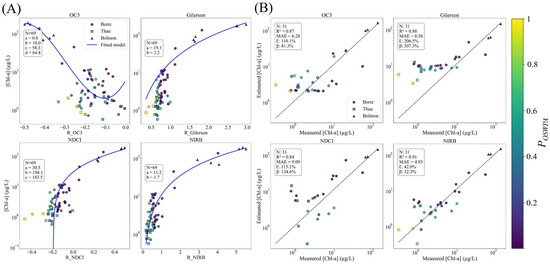
Figure 6.
Calibration (A) and validation (B) of [chl-a] retrieval algorithms considering four [chl-a] retrieval algorithms: CHLOC3, CHLGILERSON, CHLNDCI and CHLNIRB. Calibration and validation results were, respectively, obtained using 70% and 30% of the BIO-CAL/VAL in situ dataset, presenting similar distributions, while the color scale corresponds to the BC probability POSWPA computed using OSWPA.
In the calibration panel (Figure 6A), all four models reproduce the overall [chl-a]–reflectance relationship, but their ability to represent bottom-contaminated data varies. The OC3 model exhibits a curved response with a minimum at 2 µg/L and shows strong dispersion, especially among stations with high POSWPA. For NDCI and Gilerson, the shape of the curve also fails to capture the wide spread of bottom-contaminated points. In contrast, the NIRB model offers the most suitable curve, capturing the full dynamic range of [chl-a] with minimal sensitivity to BC, and better aligning with both low and high concentration values.
The validation panel (Figure 6B) reveals marked performance differences. OC3 tends to overestimate low [chl-a] values, with high scatter in bottom-contaminated stations (β = +41.3%, ε = 110.1%). Gilerson performs poorly overall, especially below 20 µg/L, with large overestimations (β > +300%, ε > 200%). NDCI also underperforms: several bottom-contaminated stations yield invalid (negative) [chl-a] values, while others show strong overestimation (β = +134.6%, ε = 115.1%). In contrast, the NIRB model delivers the best agreement with in situ data, maintaining low dispersion across the full range (0.5–135 µg/L), with MAE = 4.85 µg/L, ε = 42.0%, and β = +32.3%. It reduces the error by more than half compared to OC3 and NDCI, and by a factor of five compared to Gilerson, confirming its robustness in these shallow environments. Visual inspection of Figure 6A suggests that the most strongly bottom-contaminated stations (points with high OSWPA probability) are those deviating from the general relationship in OC3, NDCI, and Gilerson. This suggests that OSWPA can be used to identify such outliers, and filtering them (e.g., with a POSWPA > 0.5) would improve the performance of these classical algorithms. However, even in this case, the NIRB ratio remains consistently more robust, which further supports its suitability for these environments.
3.3.2. [SPM]
Figure 7 presents the calibration (Figure 7A) and validation (Figure 7B) results of four empirical algorithms for retrieving [SPM].
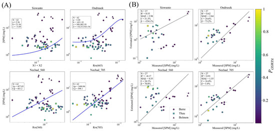
Figure 7.
Calibration (A) and validation (B) of four [SPM] retrieval algorithms (SPMSISWANTO, SPMONDRUSEK, SPMNECHAD-560, SPMNECHAD-705). Calibration and validation results were, respectively, obtained using 70% and 30% of the BIO-CAL/VAL in situ dataset, both with similar distributions of values, while the color scale corresponds to the BC probability POSWPA computed using OSWPA. Error bars are displayed for stations measured in triplicate.
In the calibration panel (Figure 7A), the algorithms exhibit contrasting behaviors. The Siswanto model, which relies on a combination of two spectral variables, shows poor agreement with in situ [SPM], with no clear relationship across the dataset. The Ondrusek model displays a non-linear response, with a plateau around 3 mg/L and an inflection point likely caused by overfitting due to the influence of bottom-contaminated stations. The Nechad model at 560 nm (Nechad-560) shows a weak slope that fails to represent bottom-contaminated stations with high Rrs(560) and low [SPM]. In contrast, the Nechad model at 705 nm (Nechad-705) displays a clear and consistent linear relationship across the dataset, indicating a better sensitivity to [SPM] and reduced sensitivity to BC.
The validation results (Figure 7B) reinforce these observations. The Siswanto model fails to reproduce [SPM] with substantial underestimation (β = −354.1%). The Ondrusek model achieves a better fit (R2 = 0.62) but remains biased, particularly overestimating low [SPM] values because of the plateau (ε = 24.6%; β = +73.2%). The Nechad-560 model shows the worst global metrics (MAE = 4.55 mg/L; ε = 34.1%; β = +70%) and no significant correlation (R2 = −0.17), primarily due to overestimation in bottom-contaminated stations. The Nechad-705 model clearly outperforms the others, with the strongest agreement between predicted and observed values (R2 = 0.91), low dispersion, and the best metrics (MAE = 1.55 mg/L; ε = 16.4%; β = +5.4%). For the lagoons considered in this study, this band represents the most suitable compromise for [SPM] retrieval, being less affected by BC than 560 and 665 nm due to stronger water absorption, while avoiding the higher noise level observed at 743 nm.
3.4. Validation and Intercomparaison of Satellite-Derived Water Quality Products
3.4.1. [Chl-a]
Figure 8 presents the validation of four satellite-derived [chl-a] algorithms (OC3, Gilerson, NDCI, and NIRB) applied to S2-MSI Rrs data obtained by applying the Sen2Cor_sc processor. The analysis relies on 160 matchups from the SWQ-VAL dataset (Supplementary Table S3). Each point represents a satellite vs. in situ comparison, with the marker shape indicating the lagoon and color scale indicating BC (POSWPA).
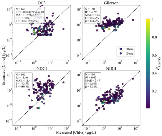
Figure 8.
Validation of satellite-derived [chl-a] products using the SWQ-VAL dataset (log–log scale). The figure shows scatterplot results for four [chl-a] retrieval algorithms (CHLOC3, CHLGILERSON, CHLNDCI, CHLNIRB) applied to S2-MSI Rrs obtained using the Sen2Cor_sc processor.
The OC3 algorithm shows very poor results, with no clear correlation and a strong overestimation of in situ measurements, especially for concentrations below 2 µg/L. This is reflected in its extremely high relative error (ε = 187%) and a bias beyond acceptable limits, confirming its inapplicability in these optically complex waters. The Gilerson model also overestimates [chl-a], particularly in the low-to-moderate range (<10 µg/L), with a bias exceeding +400 %. This pattern, already observed using the in situ results (Figure 6B), likely stems from poor calibration influenced by bottom-contaminated stations. The NDCI algorithm follows a similar trend, with substantial overestimations and a bias also above +400%. Several stations yield negative values, mostly those with high POSWPA scores, which suggest strong BC. In contrast, the NIRB model provides the most accurate relation (R2 = 0.67), with points closely aligned along the 1:1 line and lower dispersion. Its relative error (ε = 62.0%) and bias (β = +32.8%) are significantly reduced compared to the other models, highlighting the effectiveness of the NIR/blue Rrs ratio for estimating [chl-a] in optically shallow and complex environments.
Figure 9 compares [chl-a] maps produced by the same retrieval algorithms (OC3, Gilerson, NDCI, NIRB) applied to an S2-MSI scene from 9 October 2021 over the Berre lagoon. All maps (B) were derived from Rrs obtained using Sen2Cor_sc; the RGB composite (A) provides spatial context. This early autumn scene corresponds to moderate [chl-a] (~10 µg/L), consistent with in situ data collected on 18 October 2021 (2.6–21 µg/L).
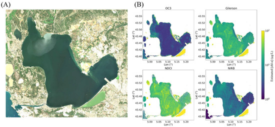
Figure 9.
(A) S2-MSI RGB composite image of the Berre lagoon acquired on 9 October 2021. (B) Comparison of [chl-a] maps generated using four empirical algorithms (CHLOC3, CHLGILERSON, CHLNDCI and CHLNIRB) applied to the same scene processed using Sen2Cor_sc.
A turbid plume from the hydroelectric canal is visible in the north, while clearer waters in the east reveal BC, especially in the “Étang de Vaïne” and over the central sandy bar (Figure 9A).
The OC3 algorithm strongly underestimates [chl-a] across most of the lagoon (Figure 9B), with very low and spatially uniform values. In contrast, it shows extreme overestimations in bottom-contaminated OSWs such as the sandy bar and in some parts of the “Étang de Vaïne”, highlighting the model’s instability and high sensitivity to BC. The Gilerson model overestimates [chl-a] throughout most of the lagoon, producing unrealistic high concentrations. In bottom-contaminated areas, the algorithm tends to underestimate values due to the attenuation of the Rrs(705)/Rrs(665) ratio due to strong BC. The NDCI model behaves similarly to Gilerson, but with even higher [chl-a] estimates. It also produces negative values (white pixels) in areas affected by BC (sandy bar and “Étang de Vaïne”), as already observed in Figure 8. These artifacts further emphasize the model’s poor reliability in OSWs. In contrast, the NIRB model yields the most consistent and realistic results. Concentrations range from 2 to 25 µg/L, with strong visible gradients. These spatial patterns match well with known biogeochemical conditions during the period and confirm the robustness of the NIRB algorithm in these optically complex waters.
3.4.2. [SPM]
Figure 10 presents the validation of the four [SPM] retrieval algorithms (Siswanto, Ondrusek, Nechad-560, Nechad-705) applied to S2-MSI Rrs data generated using Sen2Cor_sc. The analysis relies on 129 matchups from the SWQ-VAL dataset (Supplementary Table S3). Each point corresponds to a satellite vs. in situ matchup, with the color scale indicating BC (POSWPA).
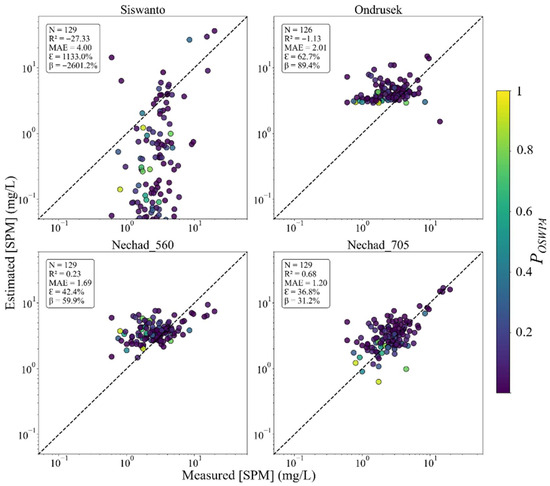
Figure 10.
Validation of satellite-derived [SPM] products using the SWQ-VAL dataset (log–log scale). The figure shows the scatterplots of four [SPM] retrieval models (SPMSISWANTO, SPMONDRUSEK, SPMNECHAD-555, SPMNECHAD-705) applied to S2-MSI satellite Rrs data generated using Sen2Cor_sc.
The Siswanto model shows very poor agreement with field data, largely underestimating [SPM] and showing no correlation (R2 = −27.33; β = −2601.2%). This strong underestimation was also observed in Figure 7B and is likely due to the use of a complex multi-band index involving wavelengths highly affected by BC, which results in poor calibration. The Ondrusek model also fails to accurately retrieve [SPM]. Its polynomial structure imposes a saturation effect below 3 mg/L, leading to systematic overestimation of low values. Some predictions are missing due to negative outputs, and the correlation remains non-existent (R2 = −1.13; β = +89.4%). The Nechad-560 model performs moderately better, with reduced dispersion and a modest correlation (R2 = 0.23), but still shows systematic overestimation (β = +59.9%), particularly for low [SPM] values and bottom-contaminated stations. As already observed in Figure 7B, the Nechad-705 model gives the best results, with a good agreement (R2 = 0.68), the lowest error (ε = 36.8%), bias (β = +31.2%), and MAE (1.20 mg/L).
Figure 11 shows [SPM] maps produced using the same retrieval algorithms (Siswanto, Ondrusek, Nechad-560, Nechad-705) applied to an S2-MSI image acquired on 22 February 2019 over the Berre lagoon (Figure 11B). The RGB composite (Figure 11A) provides spatial context. Rrs data were generated using the Sen2Cor_sc processor.
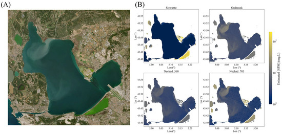
Figure 11.
(A) S2-MSI RGB composite image of the Berre lagoon acquired on 22 February 2019. (B) Comparison of [SPM] maps generated using four empirical algorithms (SPMSISWANTO, SPMONDRUSEK, SPMNECHAD-555, SPMNECHAD-705) applied to the same scene after Sen2Cor_sc.
The scene, typical of winter conditions, is marked by generally clear waters, a pronounced turbid plume from the hydroelectric canal in the north, and a more diffuse plume extending into the central lagoon (Figure 11A). In parallel, high water transparency in areas like the “Étang de Vaïne” and the shallow sandy bar reveals strong BC, offering favorable conditions to assess the algorithm sensitivity to turbidity and BC.
The Siswanto algorithm fails to detect the plumes and predicts minimal concentrations across most of the lagoon (Figure 11B), except in some very shallow areas within the “Étang de Vaïne”, where higher values are limited to zones close to the shoreline. It also largely overestimates [SPM] in Bolmon, where true concentrations are typically around 25 mg/L. The Ondrusek model better captures the main plume, with realistic values in the northern and central parts of the lagoon. However, it produces low to negative outputs in the most turbid areas of the panache, visible as blue (low) and white (negative) pixels. Outside the plume, the model assigns a constant baseline concentration close to 3 mg/L, leading to clear overestimations in clear waters. The Nechad-560 model performs consistently but still underestimates [SPM] in the plume and Bolmon lagoon. High overestimations remain in bottom-contaminated areas, reflecting the persistent sensitivity of the 560 nm band to BC, as already observed in Figure 10. In contrast, the Nechad-705 model provides the most realistic [SPM] distribution. It captures both plumes with concentrations ranging from 6 to 35 mg/L, reproduces well the contrast with the clear waters of “Étang de Vaïne”, and provides consistent values in the Bolmon lagoon. While slight pixel-level noise is present due to the use of the 705 nm band, the algorithm captures the main spatial features with the best contrast and minimal BC.
4. Discussion
This study aimed to develop and validate a satellite-based processing chain for monitoring WQ parameters in optically shallow coastal lagoons using S2-MSI data. The approach focused on three main objectives: (i) evaluating AC processors for accurate Rrs retrieval, (ii) developing OSWPA to detect BC and differentiating OSWs from ODWs, and (iii) assessing bio-optical algorithms for estimating [chl-a] and [SPM] from both in situ and satellite-derived Rrs. These objectives were addressed using comprehensive datasets from the Berre, Thau, and Bolmon lagoons, which display contrasting bio-optical conditions. The overall goal was to identify accurate and operational solutions suitable for the specific challenges of optically shallow coastal lagoons.
4.1. Performance of Atmospheric Corrections
Coastal lagoons present major challenges for AC due to their optical complexity. Our results show that combining Sen2Cor with the NIR similarity correction (Sen2Cor_sc) [58] provides the best overall performance, with relative errors below 30% across all bands and low bias. This improvement stems from the NIR-SC’s ability to correct for residual skylight reflection, sunglint, and adjacency effects by enforcing a water-like spectral shape in the NIR. Compared to [39], who reported errors ranging from 35% to 80% in coastal and inland waters depending on the AC, wavelength, and water type, our results are at least comparable, if not better, despite the optical complexity of the Berre and Thau lagoons.
These findings are consistent with previous studies showing that Sen2Cor can provide reliable performance in inland and lagoon waters [19,29,88,89,90]. They also align with [91], who evaluated several ACs over the Berre lagoon using HYPERNETS data. Their results showed that ACs which include a sunglint correction (ACOLITE_glint, polymer, GRS) yielded the best performance, while Sen2Cor alone introduced a strong positive bias, likely due to uncorrected skylight reflection, sunglint, and adjacency effects. However, our results demonstrate that applying a simple NIR similarity correction to Sen2Cor outputs is sufficient to mitigate such effects and can even outperform more advanced AC methods. This highlights both the robustness and the operational potential of this straightforward approach.
This NIR-SC, however, has some limitations, as it remains valid mainly in clear to moderately turbid waters and may fail under extreme turbidity [87] or strong adjacency effects. In such cases, alternative methods such as the T-Mart approach [92] or RAdCor [93] appear promising. Nonetheless, since such extreme turbidity levels (>300 mg/L) are rarely encountered in coastal lagoons, the Sen2Cor_sc combination can be considered a broadly applicable and operational solution for these environments.
In conclusion, while more sophisticated ACs exist, our study suggests that a simple NIR-SC applied to standard Sen2Cor outputs offers a practical and effective solution for retrieving accurate Rrs(λ) in optically complex coastal lagoons. This is especially valuable given the native availability of Sen2Cor Level-2A products via the Copernicus program, avoiding the complexity of integrating less accessible, non-operational AC methods into automated processing chains.
4.2. Detection of Bottom Contamination with OSWPA
OSWPA effectively detected BC under diverse bio-optical conditions (Figure 4). By combining two spectral reflectance ratios (RBG and RNIRG), the algorithm distinguishes OSWs from ODWs, even in the presence of turbid plumes or phytoplankton blooms. In addition to the visual validations of Figure 4, OSWPA was also quantitatively evaluated: POSWPA values decreased with increasing water depth (Supplementary Figure S4), consistent with the expected reduction in BC. This is in line with the well-established use of the RBG in satellite-derived bathymetry products [60,94,95,96,97] and previous works that linked low RBG values to BC [61]. However, this ratio alone is sensitive to the concentration and composition of optically active water constituents: high [chl-a], [SPM], or [CDOM] can impact RBG and hence induce confusion with BC (Figure 3). To resolve this ambiguity, RNIRG is used as a proxy for SPM or chl-a load, improving discrimination in dynamic environments where OSWs and ODWs coexist.
Compared to existing approaches, OSWPA shows improved robustness across diverse bio-optical settings. Simpler methods based on thresholding the blue-to-green reflectance ratio are prone to misclassifying turbid or bloom-affected waters as OSWs [60]. NIR-based indices such as NIBEI [41,59], though more sensitive to very shallow bottoms, are often affected by adjacency effects in the NIR bands. Over our study sites, NIBEI failed to detect BC reliably, likely detecting adjacency effects instead of BC.
More advanced methods like the Substratum Detectability Index (SDI) [63,64], which compare observed and modelled spectra, often require hyperspectral input and intensive computation, limiting their applicability to high-resolution multispectral sensors. Machine-learning approaches have also been proposed [46], but their performance and transferability depend on the training datasets. In our lagoons, the recent DNNs of [46] often misclassified turbid plumes as BC, whereas OSWPA was explicitly designed to avoid such confusion (see Supplementary Figure S3).
The novelty of OSWPA lies in its combination of a probabilistic framework with a solid bio-optical basis. Thresholds are derived from forward simulations [45], meaning that only approximate ranges of [chl-a], [SPM], [CDOM], and substrate types are required to recalibrate the method. In practice, we recommend applying a probability threshold of 0.5 to generate a binary OSW/ODW mask, which provides the most consistent results in our tests (see Supplementary Figure S2 for example).
Yet, some limitations remain. The RBG and RNIRG thresholds were empirically tuned from our lagoons and may not directly apply elsewhere. In very shallow waters (<1 m), such as in the “crique de l’Angle” (Figure 4), BC can lower RNIRG and lead to misclassification. Replacing the 705 nm band with a wavelength exhibiting a higher water absorption (e.g., 743 nm) could help reduce this bias. Nevertheless, OSWPA’s adaptability is a key strength: in our case, parameters calibrated for Berre and Thau also performed well in the Bizerte lagoon (Figure S2), supporting their use as a transferable starting point for similar environments.
4.3. Performance of [Chl-a] and [SPM] Retrieval Algorithms
Retrieving both [chl-a] and [SPM] in optically shallow coastal lagoons presents similar challenges due to BC and the variability of optically active constituents. We evaluated four algorithms for each parameter using both in situ and S2-MSI Rrs.
For [chl-a], the NIRB model based on the Rrs(705)/Rrs(443) ratio clearly outperformed the others on both in situ and satellite datasets, reducing errors by a factor of ~2–3 compared to traditional OC3 and NDCI algorithms, and consistently improving correlation (Figure 6 and Figure 8). To our knowledge, this ratio has not been previously described in the literature. Its success likely stems from its bio-optical consistency and reduced sensitivity to BC (Figure 5). Unlike classical algorithms relying on red or green wavelengths, which are more strongly affected by BC, the combination of blue (443 nm) and NIR (705 nm) bands offers a more stable optical window. The blue band is influenced by absorption from both phytoplankton and CDOM, but is less sensitive to BC than green or red wavelengths, as previously highlighted by [40]. In contrast, the NIR band is strongly absorbed by water yet remains sensitive to phytoplankton-induced backscattering. As [chl-a] increases, Rrs(705) rises while Rrs(443) decreases, enhancing the sensitivity of the ratio even at low concentrations. Conversely, retrieval algorithms based on the red/NIR Rrs ratios require higher [chl-a] levels to generate detectable signals, due to weaker pigment absorption in the red. This dual sensitivity, combined with the reduced BC on both selected bands, likely explains the superior performance of the NIRB model in our study sites. Although this algorithm was calibrated on our dataset, its spectral rationale is bio-optically consistent and should remain valid in other lagoonal or inland waters, provided that the coefficients are recalibrated to account for local optical conditions.
On in situ data, the NIRB algorithm achieved a relative error of ~40% with a strong correlation (R2 = 0.91), comparable to previous studies in optically complex waters [70,98,99]. Applied to satellite-derived Rrs, the error rose to ~60% and R2 dropped to 0.67, still within acceptable ranges for such environments [19,99,100]. This decrease reflects known uncertainties: temporal mismatch with field sampling [101], sub-pixel heterogeneity, and AC errors, particularly at 443 and 705 nm, where the Rrs uncertainty can exceed 30% (Figure 2). The performance is slightly lower than that reported in [29,102], where relative errors of ~43% on satellite data and RMSE of 15–25% on in situ data were obtained. However, those studies focused on eutrophic inland waters with high [chl-a] and minimal BC, where the phytoplankton signal dominates. In contrast, our study sites are oligotrophic to mesotrophic with lower pigment levels, leading to weaker Rrs signals and stronger interference with BC and other constituents like SPM and CDOM.
For [SPM], the Siswanto and Nechad-560 models performed poorly, reflecting the limitations of the blue, green and red bands in shallow coastal waters for estimating [SPM]. These wavelengths are strongly affected by BC [40] and other water constituents such as CDOM and chl-a, reducing their reliability in complex optical conditions where no specific constituent dominates the signal. In particular, the green band is sensitive to both CDOM absorption, saturation effects [75], and BC, which explains the weak correlation and overestimations in OSWs (Figure 10 and Figure 11). The Ondrusek model, based on the 665 nm band, performed poorly due to its empirical polynomial nature and poor calibration, likely driven by the high sensitivity of the 665 nm band to both BC and phytoplankton absorption. In contrast, the Nechad-705 algorithm proved to be the most reliable in our study sites, as the 705 nm band is less affected by BC due to strong water absorption, and less influenced by CDOM or chl-a absorption—particularly relevant given that SPM here is largely phytoplankton-driven (≈50% on average). This explains the strong agreement with in situ data and the consistent spatial patterns observed in satellite-derived maps (Figure 10 and Figure 11). The algorithm is semi-analytical, and our calibrated coefficient (Ap = 1488) remains close to the generic value reported by [76] (Ap = 1550), suggesting good transferability while still requiring recalibration in lagoon systems with different optical properties, such as those dominated by mineral particles.
The observed error (ε = 36.8%) for Nechad-705 compares favorably with other studies on satellite-based [SPM] retrieval. Most recent assessments report higher relative errors [103,104] often exceeding 45–50%, particularly when applied to broader [SPM] ranges or different sensors with lower spatial resolution, such as Sentinel-3 Ocean and Land Color Instrument (OLCI) [105]. The relatively low [SPM] range (0.9–21 mg/L) in our dataset likely contributed to the improved accuracy.
Together, the NIRB and Nechad-705 algorithms highlight the critical importance of the blue (443 nm) and NIR (705 nm) bands for retrieving both [chl-a] and [SPM] in optically complex shallow environments. Their semi-empirical nature facilitates recalibration and integration into operational workflows.
4.4. Limitations and Perspectives
Despite the promising results, some limitations should be acknowledged. First, validation was restricted to two Mediterranean lagoon systems, and extreme optical conditions (e.g., intense sediment resuspension or turbid freshwater inputs) may not be fully captured. The RBG and RNIRG thresholds used in OSWPA were empirically tuned for Berre and Thau lagoons, and may require recalibration elsewhere, particularly in very shallow (<1 m) or CDOM-rich environments. Likewise, the retrieval models for [chl-a] and [SPM] were optimized for local conditions and should probably be recalibrated when applied to other sites or bio-optical contexts. While their semi-empirical but physically consistent design facilitates such adaptation, expanding the application of these algorithms to additional sites would enhance the generalizability and relevance of the approach.
Another limitation is the absence of explicit CDOM measurements, although this constituent could strongly affect coastal waters. Incorporating CDOM, as well as transparency-related indicators such as Secchi depth, would represent a natural extension of this work. Finally, while S2-MSI proved suitable, hyperspectral missions (e.g., PRISMA, EnMAP) could refine threshold selection and improve the robustness of OSWPA and bio-optical retrievals.
Overall, the modular structure of the workflow ensures adaptability: each component (AC, OSWPA, inversion algorithms) can be recalibrated for different sites and conditions, supporting its transferability to other lagoon systems.
5. Conclusions and Perspectives
This study presents an operational satellite-based workflow for monitoring WQ in optically shallow coastal lagoons using S2-MSI data. By combining a simple supplementary correction (NIR-SC), a novel BC detection algorithm (OSWPA), and retrieval models for [chl-a] and [SPM], the approach delivers accurate, spatially robust estimates from standard Level-2A products, even under challenging conditions.
A key finding is the central role of the 705 nm band for retrieving both [chl-a] and [SPM] in complex lagoon waters. The newly developed NIRB algorithm for [chl-a], based on the Rrs(705)/Rrs(443) ratio, outperformed traditional approaches and offers a promising, bio-optically consistent model for OSWs. Similarly, the Nechad-705 model was confirmed as the most reliable option for [SPM], thanks to its reduced sensitivity to BC and other confounding constituents. Another important contribution is OSWPA, which combines two spectral ratios within a probabilistic framework to detect OSWs and quantify BC. Its design ensures both physical consistency and operational practicality, while allowing straightforward recalibration for different environments.
Altogether, the workflow provides accurate, interpretable, and cost-effective monitoring tools that complement in situ programs required under the EU Water Framework Directive for coastal lagoons. By filling spatial and temporal observation gaps in key WQ indicators, it strengthens both ecological risk detection and long-term assessment efforts and offers a solid basis for future integration into semi-automated monitoring systems.
Supplementary Materials
The following supporting information can be downloaded at: https://www.mdpi.com/article/10.3390/rs17203430/s1. Figure S1: Comparison of Rrs signals obtained by the TRIOS sensors and the HYPERNETS system on station H1; Figure S2: Illustration of the OSWPA approach applied to Bizerte Lagoon (Tunisia) on an S2-MSI image of 24 December 2021 (bathymetric map from [106]); Figure S3: Comparison between OSWPA and DNNs [46] methods for the detection of OSWs in the Berre Lagoon (1 September 2021); Figure S4: Validation of OSWPA against bathymetry in the Berre Lagoon (S2-MSI image, 30 April 2025); Table S1: Optical parameters and substrate types used for the simulation of OSW and ODW spectra using the Lee model [45] for the development of OSWPA; Table S2: Descriptive statistics of the BIO-CAL/VAL in situ datasets; Table S3: Summary of the campaigns and datasets used for algorithms calibration and validation.
Author Contributions
S.M. conceived the study, developed the methodology, performed the investigation, carried out the software development and data analysis, and wrote the original draft. D.D. supervised the work, contributed to the validation and visualization of the results, reviewed and edited the manuscript, and secured project funding. P.B. provided supervision and contributed to the critical review of the manuscript. P.G. supervised the study and provided manuscript feedback and scientific recommendations. P.R.R. contributed to field data acquisition and reviewed the manuscript. All authors have read and agreed to the published version of the manuscript.
Funding
This research was supported by Région Sud Provence-Alpes-Côte d’Azur, ACRI-ST, and CNRS, and received funding from the European Union’s Horizon 2020 research and innovation programme under grant agreement No. 775983 (HYPERNETS). Field campaigns and data processing were co-funded by the French Space Agency (CNES) through the TOSCA program (HYPERVAL project). The APC was funded by CNRS.
Data Availability Statement
The datasets and codes supporting the methodology and results presented in this study are available from the corresponding author upon reasonable request. Some in-situ data were obtained under data-use agreements with partner organizations and cannot be publicly shared.
Acknowledgments
The authors gratefully acknowledge the GIPREB (Groupement d’Intérêt Public pour la Réhabilitation de l’Étang de Berre) for their support during field campaigns and access to their in situ monitoring database. We also thank the REPHY program (Réseau de Surveillance du Phytoplancton et des Phycotoxines), coordinated byIfremer, for providing phytoplankton quality data. Fieldwork and sampling logistics on the Thau lagoon were supported by OREME (Observatoire de Recherche Méditerranéen de l’Environnement). We further acknowledge the HYPERNETS project (EU H2020 Grant No. 775983) for supplying radiometric reflectance data over the Berre and Thau lagoons. Special thanks to Tristan Harmel for the GRS-processed images, Karen Nieto Saavedra for Polymer processing of S2-MSI scenes, Diego Cardec for assistance with SPM sample analysis, and Gregory Messiaen (Ifremer) for providing the Thau bathymetry dataset. The S2-MSI Level-2A images were provided free of charge by the Copernicus Programme and downloaded via the CREODIAS platform (https://creodias.eu/, accessed on 25 February 2025), which we also thank for access and related services. Portions of the manuscript were assisted using ChatGPT (GPT-4o, OpenAI) to improve the structure, refine the abstract, enhance scientific English, and shorten the text. All AI-assisted content was carefully reviewed and validated by the authors to ensure scientific accuracy.
Conflicts of Interest
The authors declare no conflicts of interest.
Abbreviations
The following abbreviations are used in this manuscript:
| [chl-a] | Chlorophyll-a concentration |
| [SPM] | Suspended Particulate Matter concentration |
| AC | Atmospheric Correction |
| NIR | Near-infrared |
| OSWPA | Optically Shallow Water Probability Algorithm |
| BC | Bottom Contamination |
| WQ | Water Quality |
| WFD | Water Framework Directive |
| Rrs | remote-sensing reflectance |
| OSW | Optically Shallow Water |
| ODW | Optically Deep Water |
| OLI | Operational Land Imager |
| ETM+ | Enhanced Thematic Mapper Plus |
| S2-MSI | Sentinel-2 Multispectral Imager |
| GIPREB | Groupement d’Intérêt Public pour la Réhabilitation de l’Étang de Berre |
| REPHY | Réseau de Surveillance du Phytoplancton et de l’Hydrologie |
| OAC | Optically Active Constituant |
| CDOM | Colored Dissolved Organic Matter |
| IOP | Inherent Optical Property |
| POSWPA | Optically Shallow Water probability |
| β | Signed median bias |
| ε | Signed median absolute percentage error |
| R2 | Coefficient of determination |
| MAE | Mean Absolute Error |
| SWIR | Short-Wave Infrared |
| NIR-SC | Near-Infrared Similarity Correction |
| RMSE | Root Mean Square Error |
| DNNs | Deep Neural Networks |
| NIBEI | Near-Infrared Bottom Effect Index |
| SDI | Substratum Detectability Index |
| OLCI | Ocean and Land Color Instrument |
References
- Kjerfve, B. Coastal Lagoons. In Coastal Lagoon Processes; Elsevier Oceanography Series; Elsevier: Amsterdam, The Netherlands, 1994; Volume 60, pp. 1–8. [Google Scholar]
- Pérez-Ruzafa, A.; Marcos, C.; Pérez-Ruzafa, I.M. Mediterranean Coastal Lagoons in an Ecosystem and Aquatic Resources Management Context. Phys. Chem. Earth Parts A/B/C 2011, 36, 160–166. [Google Scholar] [CrossRef]
- Pérez-Ruzafa, A.; Pérez-Ruzafa, I.M.; Newton, A.; Marcos, C. Coastal Lagoons: Environmental Variability, Ecosystem Complexity, and Goods and Services Uniformity. In Coasts and Estuaries: The Future; Elsevier: Amsterdam, The Netherlands, 2019; pp. 253–276. ISBN 9780128140048. [Google Scholar]
- Cataudella, S.; Crosetti, D.; Massa, F. Mediterranean Coastal Lagoons: Sustainable Management and Interactions Among Aquaculture, Catpure Fisheries and The Environment. In Studies and Reviews General Fisheries Comission for the Mediterranean; FAO: Rome, Italy, 2015; Volume 95, pp. 1–278. [Google Scholar]
- Derolez, V.; Malet, N.; Fiandrino, A.; Lagarde, F.; Richard, M.; Ouisse, V.; Bec, B.; Aliaume, C. Fifty Years of Ecological Changes: Regime Shifts and Drivers in a Coastal Mediterranean Lagoon during Oligotrophication. Sci. Total Environ. 2020, 732, 139292. [Google Scholar] [CrossRef]
- Kennish, M.J.; Paerl, H.W. Coastal Lagoons: Critical Habitats of Environmental Change, 1st ed.; Kennish, M.J., Hans, P.W., Eds.; CRC Press: Boca Raton, FL, USA, 2010. [Google Scholar]
- Newton, A.; Brito, A.C.; Icely, J.D.; Derolez, V.; Clara, I.; Angus, S.; Schernewski, G.; Inácio, M.; Lillebø, A.I.; Sousa, A.I.; et al. Assessing, Quantifying and Valuing the Ecosystem Services of Coastal Lagoons. J. Nat. Conserv. 2018, 44, 50–65. [Google Scholar] [CrossRef]
- Pérez-Ruzafa, A.; Marcos, C.; Pérez-Ruzafa, I.M.; Pérez-Marcos, M. Coastal Lagoons: “Transitional Ecosystems” between Transitional and Coastal Waters. J. Coast. Conserv. 2011, 15, 369–392. [Google Scholar] [CrossRef]
- Derolez, V.; Soudant, D.; Malet, N.; Chiantella, C.; Richard, M.; Abadie, E.; Aliaume, C.; Bec, B. Two Decades of Oligotrophication: Evidence for a Phytoplankton Community Shift in the Coastal Lagoon of Thau (Mediterranean Sea, France). Estuar. Coast. Shelf Sci. 2020, 241, 106810. [Google Scholar] [CrossRef]
- Le Ray, J.; Bec, B.; Fiandrino, A.; Lagarde, F.; Cimiterra, N.; Raimbault, P.; Roque, C.; Rigaud, S.; Régis, J.; Mostajir, B.; et al. Impact of Anoxia and Oyster Mortality on Nutrient and Microbial Planktonic Components: A Mesocosm Study. Aquaculture 2023, 566, 739171. [Google Scholar] [CrossRef]
- Herlory, O.; Briand, M.J.; Bouchoucha, M.; Derolez, V.; Munaron, D.; Cimiterra, N.; Tomasino, C.; Gonzalez, J.-L.; Giraud, A.; Boissery, P. Directive Cadre Sur l’Eau Bassin Rhône Méditerranée Corse—Année 2021; Ifremer: Brest, France, 2022; pp. 1–89. [Google Scholar] [CrossRef]
- Derolez, V.; Bec, B.; Cimiterra, N.; Foucault, E.; Messiaen, G.; Fiandrino, A.; Malet, N.; Munaron, D.; Serais, O.; Connes, C.; et al. OBSLAG 2020—Volet Eutrophisation Lagunes Méditerranéennes (Période 2015–2020). Etat DCE de La Colonne d’eau et Du Phytoplancton, Tendance et Variabilité Des Indicateurs; Ifremer: Brest, France, 2021; pp. 1–78. Available online: https://archimer.ifremer.fr/doc/00696/80768/ (accessed on 14 July 2025).
- Grillas, P.; Ximénès, M.-C.; Giraud, O.A. Adaptation Des Grilles DCE de Qualité Nutriments et Phytoplancton (Abondance et Biomasse) Pour Les Lagunes Oligo et Mésohalines; Ifremer: Brest, France, 2016; pp. 1–42. Available online: https://archimer.ifremer.fr/doc/00357/46818/ (accessed on 14 July 2025).
- Gholizadeh, M.; Melesse, A.; Reddi, L. A Comprehensive Review on Water Quality Parameters Estimation Using Remote Sensing Techniques. Sensors 2016, 16, 1298. [Google Scholar] [CrossRef]
- Giardino, C.; Brando, V.E.; Gege, P.; Pinnel, N.; Hochberg, E.; Knaeps, E.; Reusen, I.; Doerffer, R.; Bresciani, M.; Braga, F.; et al. Imaging Spectrometry of Inland and Coastal Waters: State of the Art, Achievements and Perspectives. Surv. Geophys. 2019, 40, 401–429. [Google Scholar] [CrossRef]
- Bresciani, M.; Stroppiana, D.; Odermatt, D.; Morabito, G.; Giardino, C. Assessing Remotely Sensed Chlorophyll-a for the Implementation of the Water Framework Directive in European Perialpine Lakes. Sci. Total Environ. 2011, 409, 3083–3091. [Google Scholar] [CrossRef]
- Markogianni, V.; Kalivas, D.; Petropoulos, G.P.; Dimitriou, E. Modelling of Greek Lakes Water Quality Using Earth Observation in the Framework of the Water Framework Directive (WFD). Remote Sens. 2022, 14, 739. [Google Scholar] [CrossRef]
- Papathanasopoulou, E.; Simis, S.; Alikas, K.; Ansper, A.; Anttila, J.; Barillé, A.; Barillé, L.; Brando, V.; Bresciani, M.; Bučas, M.; et al. Satellite-Assisted Monitoring of Water Quality to Support the Implementation of the Water Framework Directive; Plymouth Marine Laboratory: Plymouth, UK, 2019. [Google Scholar] [CrossRef]
- Ansper, A.; Alikas, K. Retrieval of Chlorophyll a from Sentinel-2 MSI Data for the European Union Water Framework Directive Reporting Purposes. Remote Sens. 2018, 11, 64. [Google Scholar] [CrossRef]
- Antoine, D.; Andrt, J.M.; Morel, A. Oceanic Primary Production: 2. Estimation at Global Scale from Satellite (Coastal Zone Color Scanner) Chlorophyll. Glob. Biogeochem. Cycles 1996, 10, 57–69. [Google Scholar] [CrossRef]
- Gordon, H.R.; Clark, D.K.; Mueller, J.L.; Hovis, W.A. Phytoplankton Pigments from the Nimbus-7 Coastal Zone Color Scanner: Comparisons with Surface Measurements. Science 1980, 210, 63–66. [Google Scholar] [CrossRef] [PubMed]
- Morel, A.; Prieur, L. Analysis of Variations in Ocean Color1. Limnol. Oceanogr. 1977, 22, 709–722. [Google Scholar] [CrossRef]
- Palmer, S.C.J.; Kutser, T.; Hunter, P.D. Remote Sensing of Inland Waters: Challenges, Progress and Future Directions. Remote Sens. Environ. 2015, 157, 1–8. [Google Scholar] [CrossRef]
- Braga, C.Z.F.; Vianna, M.L.; Kjerfve, B. Environmental Characterization of a Hypersaline Coastal Lagoon from Landsat-5 Thematic Mapper Data. Int. J. Remote Sens. 2003, 24, 3219–3234. [Google Scholar] [CrossRef]
- Caballero, I.; Roca, M.; Santos-echeandía, J.; Bernárdez, P.; Navarro, G. Use of the Sentinel-2 and Landsat-8 Satellites for Water Quality Monitoring: An Early Warning Tool in the Mar Menor Coastal Lagoon. Remote Sens. 2022, 14, 2744. [Google Scholar] [CrossRef]
- Erena, M.; Domínguez, J.A.; Aguado-Giménez, F.; Soria, J.; García-Galiano, S. Monitoring Coastal Lagoon Water Quality through Remote Sensing: The Mar Menor as a Case Study. Water 2019, 11, 1468. [Google Scholar] [CrossRef]
- Markogianni, V.; Dimitriou, E.; Karaouzas, I. Water Quality Monitoring and Assessment of an Urban Mediterranean Lake Facilitated by Remote Sensing Applications. Environ. Monit. Assess. 2014, 186, 5009–5026. [Google Scholar] [CrossRef]
- Mortula, M.; Ali, T.; Bachir, A.; Elaksher, A.; Abouleish, M. Towards Monitoring of Nutrient Pollution in Coastal Lake Using Remote Sensing and Regression Analysis. Water 2020, 12, 1954. [Google Scholar] [CrossRef]
- Tavares, M.H.; Lins, R.C.; Harmel, T.; Fragoso, C.R.; Martínez, J.M.; Motta-Marques, D. Atmospheric and Sunglint Correction for Retrieving Chlorophyll-a in a Productive Tropical Estuarine-Lagoon System Using Sentinel-2 MSI Imagery. ISPRS J. Photogramm. Remote Sens. 2021, 174, 215–236. [Google Scholar] [CrossRef]
- Volpe, V.; Silvestri, S.; Marani, M. Remote Sensing Retrieval of Suspended Sediment Concentration in Shallow Waters. Remote Sens. Environ. 2011, 115, 44–54. [Google Scholar] [CrossRef]
- Sòria-Perpinyà, X.; Vicente, E.; Urrego, P.; Pereira-Sandoval, M.; Ruíz-Verdú, A.; Delegido, J.; Soria, J.M.; Moreno, J. Remote Sensing of Cyanobacterial Blooms in a Hypertrophic Lagoon (Albufera of València, Eastern Iberian Peninsula) Using Multitemporal Sentinel-2 Images. Sci. Total Environ. 2020, 698, 134305. [Google Scholar] [CrossRef]
- Molner, J.V.; Soria, J.M.; Pérez-González, R.; Sòria-Perpinyà, X. Measurement of Turbidity and Total Suspended Matter in the Albufera of Valencia Lagoon (Spain) Using Sentinel-2 Images. J. Mar. Sci. Eng. 2023, 11, 1894. [Google Scholar] [CrossRef]
- Sòria-Perpinyà, X.; Miracle, M.R.; Soria, J.; Delegido, J.; Vicente, E. Remote Sensing Application for the Study of Rapid Flushing to Remediate Eutrophication in Shallow Lagoons (Albufera of Valencia). Hydrobiologia 2019, 829, 125–132. [Google Scholar] [CrossRef]
- Loisel, H.; Vantrepotte, V.; Jamet, C.; Ngoc Dat, D. Challenges and New Advances in Ocean Color Remote Sensing of Coastal Waters. In Topics in Oceanography; IntechOpen: London, UK, 2013; pp. 89–132. [Google Scholar]
- Ogashawara, I.; Mishra, D.R.; Gitelson, A.A. Remote Sensing of Inland Waters: Background and Current State-of-the-Art. In Bio-optical Modeling and Remote Sensing of Inland Waters; Elsevier: Amsterdam, The Netherlands, 2017; pp. 1–24. ISBN 9780128046548. [Google Scholar]
- Sebastiá-Frasquet, M.T.; Aguilar-Maldonado, J.A.; Santamaría-Del-ángel, E.; Estornell, J. Sentinel 2 Analysis of Turbidity Patterns in a Coastal Lagoon. Remote Sens. 2019, 11, 2926. [Google Scholar] [CrossRef]
- Balasubramanian, S.V.; Pahlevan, N.; Smith, B.; Binding, C.; Schalles, J.; Loisel, H.; Gurlin, D.; Greb, S.; Alikas, K.; Randla, M.; et al. Robust Algorithm for Estimating Total Suspended Solids (TSS) in Inland and Nearshore Coastal Waters. Remote Sens. Environ. 2020, 246, 111768. [Google Scholar] [CrossRef]
- Moses, W.J.; Sterckx, S.; Montes, M.J.; De Keukelaere, L.; Knaeps, E. Atmospheric Correction for Inland Waters. In Bio-optical Modeling and Remote Sensing of Inland Waters; Elsevier Inc.: Amsterdam, The Netherlands, 2017; pp. 69–100. ISBN 9780128046548. [Google Scholar]
- Pahlevan, N.; Mangin, A.; Balasubramanian, S.V.; Smith, B.; Alikas, K.; Arai, K.; Barbosa, C.; Bélanger, S.; Binding, C.; Bresciani, M.; et al. ACIX-Aqua: A Global Assessment of Atmospheric Correction Methods for Landsat-8 and Sentinel-2 over Lakes, Rivers, and Coastal Waters. Remote Sens. Environ. 2021, 258, 112366. [Google Scholar] [CrossRef]
- Cannizzaro, J.P.; Carder, K.L. Estimating Chlorophyll a Concentrations from Remote-Sensing Reflectance in Optically Shallow Waters. Remote Sens. Environ. 2006, 101, 13–24. [Google Scholar] [CrossRef]
- Arabi, B.; Salama, M.S.; van der Wal, D.; Pitarch, J.; Verhoef, W. The Impact of Sea Bottom Effects on the Retrieval of Water Constituent Concentrations from MERIS and OLCI Images in Shallow Tidal Waters Supported by Radiative Transfer Modeling. Remote Sens. Environ. 2020, 237, 111596. [Google Scholar] [CrossRef]
- Kutser, T.; Hedley, J.; Giardino, C.; Roelfsema, C.; Brando, V.E. Remote Sensing of Shallow Waters—A 50 Year Retrospective and Future Directions. Remote Sens. Environ. 2020, 240, 111619. [Google Scholar] [CrossRef]
- Lee, Z.; Casey, B.; Arnone, R.A.; Weidemann, A.D.; Parsons, R.; Montes, M.J.; Gao, B.-C.; Goode, W.; Davis, C.O.; Dye, J. Water and Bottom Properties of a Coastal Environment Derived from Hyperion Data Measured from the EO-1 Spacecraft Platform. J. Appl. Remote Sens. 2007, 1, 011502. [Google Scholar] [CrossRef]
- Albert, A.; Mobley, C.; Gordon, H.; Brown, O.; Evans, R.; Brown, J.; Smith, R.; Baker, K.; Clark, D. An Analytical Model for Subsurface Irradiance and Remote Sensing Reflectance in Deep and Shallow Case-2 Waters. Opt. Express 2003, 11, 2873–2890. [Google Scholar] [CrossRef] [PubMed]
- Lee, Z.; Carder, K.L.; Mobley, C.D.; Steward, R.G.; Patch, J.S. Hyperspectral Remote Sensing for Shallow Waters. I. A Semianalytical Model. Appl. Opt. 1998, 37, 6329–6338. [Google Scholar] [CrossRef]
- Richardson, G.; Foreman, N.; Knudby, A.; Wu, Y.; Lin, Y. Global Deep Learning Model for Delineation of Optically Shallow and Optically Deep Water in Sentinel-2 Imagery. Remote Sens. Environ. 2024, 311, 114302. [Google Scholar] [CrossRef]
- Bernard, G.; Boudouresque, C.F.; Picon, P. Long Term Changes in Zostera Meadows in the Berre Lagoon (Provence, Mediterranean Sea). Estuar. Coast. Shelf Sci. 2007, 73, 617–629. [Google Scholar] [CrossRef]
- Mayot, N.; De Lary, H.; Gisel, R. Rapport Du Suivi Écologique Du GIPREB: Observatoire Du Milieu 2023; GIPREB: Berre-l’Étang, France, 2024. [Google Scholar]
- Minghelli-Roman, A.; Laugier, T.; Polidori, L.; Mathieu, S.; Loubersac, L.; Gouton, P. Satellite Survey of Seasonal Trophic Status and Occasional Anoxic “malaïgue” Crises in the Thau Lagoon Using MERIS Images. Int. J. Remote Sens. 2011, 32, 909–923. [Google Scholar] [CrossRef]
- Ifremer; ODE/VIGIES; Coordination REPHY & Cellule Quadrige. Manuel Pour L’utilisation des Données REPHY. In Informations Destinées à Améliorer la Compréhension des Fichiers de Données REPHY Mis à Disposition des Scientifiques et du Public; Ifremer: Brest, France, 2017; Available online: https://archimer.ifremer.fr/doc/00409/52016/ (accessed on 14 July 2025).
- Lizotte, M.; Juhls, B.; Matsuoka, A.; Massicotte, P.; Mével, G.; Anikina, D.O.J.; Antonova, S.; Bécu, G.; Béguin, M.; Bélanger, S.; et al. Nunataryuk Field Campaigns: Understanding the Origin and Fate of Terrestrial Organic Matter in the Coastal Waters of the Mackenzie Delta Region. Earth Syst. Sci. Data 2023, 15, 1617–1653. [Google Scholar] [CrossRef]
- Ody, A.; Doxaran, D.; Verney, R.; Bourrin, F.; Morin, G.P.; Pairaud, I.; Gangloff, A. Ocean Color Remote Sensing of Suspended Sediments along a Continuum from Rivers to River Plumes: Concentration, Transport, Fluxes and Dynamics. Remote Sens. 2022, 14, 2026. [Google Scholar] [CrossRef]
- Ras, J.; Claustre, H.; Uitz, J. Spatial Variability of Phytoplankton Pigment Distributions in the Subtropical South Pacific Ocean: Comparison between in Situ and Predicted Data. Biogeosciences 2008, 5, 353–369. [Google Scholar] [CrossRef]
- Mobley, C.D. Estimation of the Remote-Sensing Reflectance from above-Surface Measurements. Appl. Opt. 1999, 38, 7442–7455. [Google Scholar] [CrossRef]
- Renosh, P.R.; Doxaran, D.; De Keukelaere, L.; Gossn, J.I. Evaluation of Atmospheric Correction Algorithms for Sentinel-2-MSI and Sentinel-3-OLCI in Highly Turbid Estuarine Waters. Remote Sens. 2020, 12, 1285. [Google Scholar] [CrossRef]
- Ruddick, K.G.; De Cauwer, V.; Park, Y.J.; Moore, G. Seaborne Measurements of near Infrared Water-Leaving Reflectance: The Similarity Spectrum for Turbid Waters. Limnol. Oceanogr. 2006, 51, 1167–1179. [Google Scholar] [CrossRef]
- Goyens, C.; Lavigne, H.; Dille, A.; Vervaeren, H. Using Hyperspectral Remote Sensing to Monitor Water Quality in Drinking Water Reservoirs. Remote Sens. 2022, 14, 5607. [Google Scholar] [CrossRef]
- Ruddick, K.; De Cauwer, V.; Van Mol, B. Use of the near Infrared Similarity Reflectance Spectrum for the Quality Control of Remote Sensing Data. In Proceedings of the Remote Sensing of the Coastal Oceanic Environment, SPIE, San Diego, CA, USA, 18 August 2005; Volume 5885, p. 588501. [Google Scholar]
- Arabi, B.; Moradi, M.; Zandler, H.; Samimi, C.; Verhoef, W. Developing a Novel Index for Detection of Optically Shallow Waters Using Multispectral Satellite Imagery and Radiative Transfer Modelling. Int. J. Remote Sens. 2024, 45, 4788–4819. [Google Scholar] [CrossRef]
- Caballero, I.; Stumpf, R.P. Confronting Turbidity, the Major Challenge for Satellite-Derived Coastal Bathymetry. Sci. Total Environ. 2023, 870, 161898. [Google Scholar] [CrossRef]
- Lee, C.B.; Traganos, D.; Reinartz, P. A Simple Cloud-Native Spectral Transformation Method to Disentangle Optically Shallow and DeepWaters in Sentinel-2 Images. Remote Sens. 2022, 14, 590. [Google Scholar] [CrossRef]
- Lee, Z.; Carder, K.L.; Mobley, C.D.; Steward, R.G.; Patch, J.S. Hyperspectral Remote Sensing for Shallow Waters: 2. Deriving Bottom Depths and Water Properties by Optimization. Appl. Opt. 1999, 38, 3831–3843. [Google Scholar] [CrossRef]
- Brando, V.E.; Anstee, J.M.; Wettle, M.; Dekker, A.G.; Phinn, S.R.; Roelfsema, C. A Physics Based Retrieval and Quality Assessment of Bathymetry from Suboptimal Hyperspectral Data. Remote Sens. Environ. 2009, 113, 755–770. [Google Scholar] [CrossRef]
- Giardino, C.; Candiani, G.; Bresciani, M.; Lee, Z.; Gagliano, S.; Pepe, M. BOMBER: A Tool for Estimating Water Quality and Bottom Properties from Remote Sensing Images. Comput. Geosci. 2012, 45, 313–318. [Google Scholar] [CrossRef]
- Lai, W.; Lee, Z.; Wang, J.; Wang, Y.; Garcia, R.; Zhang, H. A Portable Algorithm to Retrieve Bottom Depth of Optically Shallow Waters from Top-Of-Atmosphere Measurements. J. Remote Sens. 2022, 2022, 9831947. [Google Scholar] [CrossRef]
- Fry, E.S.; Pope, R.M. Absorption Spectrum (380–700 Nm) of Pure Water. II. Integrating Cavity Measurements. Appl. Opt. 1997, 36, 8710–8723. [Google Scholar] [CrossRef]
- Chylek, P.; Labrie, D.; Kou, L. Refractive Indices of Water and Ice in the 0.65- to 2.5-Μm Spectral Range. Appl. Opt. 1993, 32, 3531–3540. [Google Scholar] [CrossRef]
- Baker, K.S.; Smith, R.C. Optical Properties of the Clearest Natural Waters (200–800 Nm). Appl. Opt. 1981, 20, 177–184. [Google Scholar] [CrossRef]
- Dekker, A.G.; Phinn, S.R.; Anstee, J.; Bissett, P.; Brando, V.E.; Casey, B.; Fearns, P.; Hedley, J.; Klonowski, W.; Lee, Z.P.; et al. Intercomparison of Shallow Water Bathymetry, Hydro-Optics, and Benthos Mapping Techniques in Australian and Caribbean Coastal Environments. Limnol. Oceanogr. Methods 2011, 9, 396–425. [Google Scholar] [CrossRef]
- Neil, C.; Spyrakos, E.; Hunter, P.D.; Tyler, A.N. A Global Approach for Chlorophyll-a Retrieval across Optically Complex Inland Waters Based on Optical Water Types. Remote Sens. Environ. 2019, 229, 159–178. [Google Scholar] [CrossRef]
- O’Reilly, J.E.; Werdell, P.J. Chlorophyll Algorithms for Ocean Color Sensors—OC4, OC5 & OC6. Remote Sens. Environ. 2019, 229, 32–47. [Google Scholar] [CrossRef] [PubMed]
- Gilerson, A.A.; Gitelson, A.A.; Zhou, J.; Gurlin, D.; Moses, W.; Ioannou, I.; Ahmed, S.A.; Bailey, W.; Franz, B.A.; Harding, L.W.; et al. Algorithms for Remote Estimation of Chlorophyll-a in Coastal and Inland Waters Using Red and near Infrared Bands. Opt. Express 2010, 18, 24109–24125. [Google Scholar] [CrossRef]
- Mishra, S.; Mishra, D.R. Normalized Difference Chlorophyll Index: A Novel Model for Remote Estimation of Chlorophyll-a Concentration in Turbid Productive Waters. Remote Sens. Environ. 2012, 117, 394–406. [Google Scholar] [CrossRef]
- Han, B.; Loisel, H.; Vantrepotte, V.; Mériaux, X.; Bryère, P.; Ouillon, S.; Dessailly, D.; Xing, Q.; Zhu, J. Development of a Semi-Analytical Algorithm for the Retrieval of Suspended Particulate Matter from Remote Sensing over Clear to Very Turbid Waters. Remote Sens. 2016, 8, 211. [Google Scholar] [CrossRef]
- Novoa, S.; Doxaran, D.; Ody, A.; Vanhellemont, Q.; Lafon, V.; Lubac, B.; Gernez, P.; Zhang, Y.; Giardino, C.; Li, L.; et al. Atmospheric Corrections and Multi-Conditional Algorithm for Multi-Sensor Remote Sensing of Suspended Particulate Matter in Low-to-High Turbidity Levels Coastal Waters. Remote Sens. 2017, 9, 61. [Google Scholar] [CrossRef]
- Nechad, B.; Ruddick, K.G.; Park, Y. Calibration and Validation of a Generic Multisensor Algorithm for Mapping of Total Suspended Matter in Turbid Waters. Remote Sens. Environ. 2010, 114, 854–866. [Google Scholar] [CrossRef]
- Siswanto, E.; Tang, J.; Yamaguchi, H.; Ahn, Y.H.; Ishizaka, J.; Yoo, S.; Kim, S.W.; Kiyomoto, Y.; Yamada, K.; Chiang, C.; et al. Empirical Ocean-Color Algorithms to Retrieve Chlorophyll-a, Total Suspended Matter, and Colored Dissolved Organic Matter Absorption Coefficient in the Yellow and East China Seas. J. Oceanogr. 2011, 67, 627–650. [Google Scholar] [CrossRef]
- Ondrusek, M.; Stengel, E.; Kinkade, C.S.; Vogel, R.L.; Keegstra, P.; Hunter, C.; Kim, C. The Development of a New Optical Total Suspended Matter Algorithm for the Chesapeake Bay. Remote Sens. Environ. 2012, 119, 243–254. [Google Scholar] [CrossRef]
- Louis, J.; Debaecker, V.; Pflug, B.; Main-Knorn, M.; Bieniarz, J.; Mueller-Wilm, U.; Cadau, E.; Gascon, F. Sentinel-2 Sen2Cor: L2A Processor For Users. In Proceedings of the ESA Living Planet Symposium, Prague, Czech Republic, 9–13 May 2016; pp. 1–8. [Google Scholar]
- Müller-Wilm, U.; Louis, J.; Richter, R.; Gascon, F.; Niezette, M. Sentinel-2 Level 2A Prototype Processor: Architecture, Algorithms And First Results. In Proceedings of the ESA Living Planet Symposium; ESA Living Planet Symposium 2013, Edinburgh, UK, 9 September 2013. [Google Scholar]
- Vanhellemont, Q.; Ruddick, K. Atmospheric Correction of Metre-Scale Optical Satellite Data for Inland and Coastal Water Applications. Remote Sens. Environ. 2018, 216, 586–597. [Google Scholar] [CrossRef]
- Vanhellemont, Q. Adaptation of the Dark Spectrum Fitting Atmospheric Correction for Aquatic Applications of the Landsat and Sentinel-2 Archives. Remote Sens. Environ. 2019, 225, 175–192. [Google Scholar] [CrossRef]
- Tavora, J.; Jiang, B.; Kiffney, T.; Bourdin, G.; Gray, P.C.; Carvalho, L.S.; Hesketh, G.; Schild, K.M.; Souza, L.F.; Brady, D.C.; et al. Recipes for the Derivation of Water Quality Parameters Using the High-Spatial-Resolution Data from Sensors on Board Sentinel-2A, Sentinel-2B, Landsat-5, Landsat-7, Landsat-8, and Landsat-9 Satellites. J. Remote Sens. 2023, 3, 0049. [Google Scholar] [CrossRef]
- Steinmetz, F.; Deschamps, P.-Y.; Ramon, D. Atmospheric Correction in Presence of Sun Glint: Application to MERIS. Opt. Express 2011, 19, 9783–9800. [Google Scholar] [CrossRef]
- Harmel, T.; Chami, M.; Tormos, T.; Reynaud, N.; Danis, P.A. Sunglint Correction of the Multi-Spectral Instrument (MSI)-SENTINEL-2 Imagery over Inland and Sea Waters from SWIR Bands. Remote Sens. Environ. 2018, 204, 308–321. [Google Scholar] [CrossRef]
- Brockmann, C.; Doerffer, R.; Peters, M.; Kerstin, S.; Embacher, S.; Ruescas, A. Evolution of the C2RCC Neural Network for Sentinel 2 and 3 for the Retrieval of Ocean Colour Products in Normal and Extreme Optically Complex Waters. In ESA Living Planet Symposium; Ouwehand, L., Ed.; European Space Agency: Prague, Czech Republic, 2016; Volume 740, p. 54. [Google Scholar]
- Doron, M.; Bélanger, S.; Doxaran, D.; Babin, M. Spectral Variations in the Near-Infrared Ocean Reflectance. Remote Sens. Environ. 2011, 115, 1617–1631. [Google Scholar] [CrossRef]
- Maciel, D.; Novo, E.; de Carvalho, L.S.; Barbosa, C.; Júnior, R.F.; de Lucia Lobo, F. Retrieving Total and Inorganic Suspended Sediments in Amazon Floodplain Lakes: A Multisensor Approach. Remote Sens. 2019, 11, 1744. [Google Scholar] [CrossRef]
- Pereira-Sandoval, M.; Ruescas, A.; Urrego, P.; Ruiz-Verdú, A.; Delegido, J.; Tenjo, C.; Soria-Perpinyà, X.; Vicente, E.; Soria, J.; Moreno, J. Evaluation of Atmospheric Correction Algorithms over Spanish Inland Waters for Sentinel-2 Multi Spectral Imagery Data. Remote Sens. 2019, 11, 1469. [Google Scholar] [CrossRef]
- Souza Martins, V.; Clemente Faria Barbosa, C.; Augusto Sander de Carvalho, L.; Schaffer Ferreira Jorge, D.; de Lucia Lobo, F.; Márcia Leão de Moraes Novo, E.; Zhang, Y.; Giardino, C.; Li, L.; Li, X.; et al. Assessment of Atmospheric Correction Methods for Sentinel-2 MSI Images Applied to Amazon Floodplain Lakes. Remote Sens. 2017, 9, 322. [Google Scholar] [CrossRef]
- Doxaran, D.; ElKilani, B.; Corizzi, A.; Goyens, C. Validation of Satellite-Derived Water-Leaving Reflectance in Contrasted French Coastal Waters Based on HYPERNETS Field Measurements. Front. Remote Sens. 2024, 4, 1290110. [Google Scholar] [CrossRef]
- Wu, Y.; Knudby, A.; Pahlevan, N.; Lapen, D.; Zeng, C. Sensor-Generic Adjacency-Effect Correction for Remote Sensing of Coastal and Inland Waters. Remote Sens. Environ. 2024, 315, 114433. [Google Scholar] [CrossRef]
- Castagna, A.; Vanhellemont, Q. A Generalized Physics-Based Correction for Adjacency Effects. Appl. Opt. 2025, 64, 2719–2743. [Google Scholar] [CrossRef]
- Caballero, I.; Stumpf, R.P. Retrieval of Nearshore Bathymetry from Sentinel-2A and 2B Satellites in South Florida Coastal Waters. Estuar. Coast. Shelf Sci. 2019, 226, 106277. [Google Scholar] [CrossRef]
- Ashphaq, M.; Srivastava, P.K.; Mitra, D. Review of Near-Shore Satellite Derived Bathymetry: Classification and Account of Five Decades of Coastal Bathymetry Research. J. Ocean Eng. Sci. 2021, 6, 340–359. [Google Scholar] [CrossRef]
- Stumpf, R.P.; Holderied, K.; Sinclair, M. Determination of Water Depth with High-Resolution Satellite Imagery over Variable Bottom Types. Limnol. Oceanogr. 2003, 48, 547–556. [Google Scholar] [CrossRef]
- Caballero, I.; Stumpf, R.P.; Meredith, A. Preliminary Assessment of Turbidity and Chlorophyll Impact on Bathymetry Derived from Sentinel-2A and Sentinel-3A Satellites in South Florida. Remote Sens. 2019, 11, 645. [Google Scholar] [CrossRef]
- Camara Lins, R.; Martinez, J.-M.; da Motta Marques, D.; Almir Cirilo, J.; Ruberto Fragoso, C., Jr.; Zhang, Y.; Giardino, C.; Li, L.; Mishra, D.R.; Thenkabail, P.S. Assessment of Chlorophyll-a Remote Sensing Algorithms in a Productive Tropical Estuarine-Lagoon System. Remote Sens. 2017, 9, 516. [Google Scholar] [CrossRef]
- Le, C.; Hu, C.; Cannizzaro, J.; English, D.; Muller-Karger, F.; Lee, Z. Evaluation of Chlorophyll-a Remote Sensing Algorithms for an Optically Complex Estuary. Remote Sens. Environ. 2013, 129, 75–89. [Google Scholar] [CrossRef]
- Tran, M.D.; Vantrepotte, V.; Loisel, H.; Oliveira, E.N.; Tran, K.T.; Jorge, D.; Mériaux, X.; Paranhos, R. Band Ratios Combination for Estimating Chlorophyll-a from Sentinel-2 and Sentinel-3 in Coastal Waters. Remote Sens. 2023, 15, 1653. [Google Scholar] [CrossRef]
- Llodrà-Llabrés, J.; Martínez-López, J.; Postma, T.; Pérez-Martínez, C.; Alcaraz-Segura, D. Retrieving Water Chlorophyll-a Concentration in Inland Waters from Sentinel-2 Imagery: Review of Operability, Performance and Ways Forward. Int. J. Appl. Earth Obs. Geoinf. 2023, 125, 103605. [Google Scholar] [CrossRef]
- Moses, W.J.; Gitelson, A.A.; Berdnikov, S.; Povazhnyy, V. Estimation of Chlorophyll-a Concentration in Case II Waters Using MODIS and MERIS Data—Successes and Challenges. Environ. Res. Lett. 2009, 4, 045005. [Google Scholar] [CrossRef]
- Tavora, J.; Boss, E.; Doxaran, D.; Hill, P. An Algorithm to Estimate Suspended Particulate Matter Concentrations and Associated Uncertainties from Remote Sensing Reflectance in Coastal Environments. Remote Sens. 2020, 12, 2172. [Google Scholar] [CrossRef]
- Mabit, R.; Araújo, C.A.S.; Singh, R.K.; Bélanger, S. Empirical Remote Sensing Algorithms to Retrieve SPM and CDOM in Québec Coastal Waters. Front. Remote Sens. 2022, 3, 834908. [Google Scholar] [CrossRef]
- Subirade, C.; Jamet, C.; Tran, M.D.; Vantrepotte, V.; Han, B. Evaluation of Twelve Algorithms to Estimate Suspended Particulate Matter from OLCI over Contrasted Coastal Waters. Opt. Express 2024, 32, 45719–45744. [Google Scholar] [CrossRef]
- Aleya, L.; Béjaoui, B.; Dhib, A.; Ziadi, B.; Fertouna-Bellekhal, M.; Helali, M.A.; Khedhri, I.; Oueslati, W.; Ennouri, R.; Yamashita, C.; et al. Chapter 10: Tunisia. In World Seas: An Environmental Evaluation Volume I: Europe, the Americas and West Africa, 2nd ed.; Academic Press (Elsevier): London, UK, 2018; pp. 261–282. [Google Scholar] [CrossRef]


Disclaimer/Publisher’s Note: The statements, opinions and data contained in all publications are solely those of the individual author(s) and contributor(s) and not of MDPI and/or the editor(s). MDPI and/or the editor(s) disclaim responsibility for any injury to people or property resulting from any ideas, methods, instructions or products referred to in the content. |
© 2025 by the authors. Licensee MDPI, Basel, Switzerland. This article is an open access article distributed under the terms and conditions of the Creative Commons Attribution (CC BY) license (https://creativecommons.org/licenses/by/4.0/).