Highlights
What are the main findings?
- Dynamic clutter interferes with the received signal in Ground-based Interferometry.
- Through the Image plain technique the interference can be eliminated.
What is the implication of the main finding?
- Fast moving targets aliasing in doppler can be eliminated through the image plane technique.
- Fast moving target imaging can be performed as a by-product of the image plane technique.
Abstract
In this work, a radar imagery-based signal processing technique to eliminate dynamic clutter interference in Structural Health Monitoring (SHM) is proposed. This can be considered an application of a joint communication and sensing telecommunication infrastructure, leveraging a base-station as ground-based radar. The dynamic clutter is considered to be a fast moving road user, such as car, truck, or moped. The proposed technique is suitable in case of a dynamic clutter, such that its Doppler contribute alias and falls over the 0 Hz component. In those cases, a standard low-pass filter is not a viable option. Indeed, an excessively shallow low-pass filter preserves the dynamic clutter contribution, while an excessively narrow low-pass filter deletes the displacement information and also preserves the dynamic clutter. The proposed approach leverages the Time Domain Backprojection (TDBP), a well-known technique to produce radar imagery, to transfer the dynamic clutter from the data domain to an image plane, where the dynamic clutter is maximally compressed. Consequently, the dynamic clutter can be more effectively suppressed than in the range-Doppler domain. The dynamic clutter cancellation is performed by coherent subtraction. Throughout this work, a numerical simulation is conducted. The simulation results show consistency with the ground truth. A further validation is performed using real-world data acquired in the C-band by Huawei Technologies. Corner reflectors are placed on an infrastructure, in particular a bridge, to perform the measurements. Here, two case studies are proposed: a bus and a truck. The validation shows consistency with the ground truth, providing a degree of improvement within respect to the corrupted displacement on the mean error and its variance. As a by-product of the algorithm, there is the capability to produce high-resolution imagery of moving targets.
1. Introduction
Bridges and transportation infrastructure are exposed to significant aging and degradation due to high physical loads caused by traffic and harsh environmental conditions [1,2]. These factors accelerate both aging and deterioration processes, posing significant safety risks, particularly in light of the increasing utilization of such structures. Neglecting these issues can lead to catastrophic failures. A notable example is the collapse of the Morandi Bridge in Italy, which occurred in 2018 due to structural failure, resulting in numerous casualties and causing severe disruptions to the transportation network. Another relevant case is the collapse of the Carola Bridge in Germany in 2024. Despite undergoing annual inspections and exhibiting no apparent signs of degradation, the bridge unexpectedly failed, underscoring the limitations of conventional monitoring practices. Within this framework, Structural Health Monitoring (SHM) plays a pivotal role. SHM encompasses the design, development, and implementation of strategies for damage detection and characterization, enabling the real-time assessment of structural integrity and performance. SHM utilizes the information provided by an extensive network of various sensors [3], such as optical fibers, acoustic or wireless sensors, and computer vision techniques. However, the downside of this approach is that the deployment and maintenance of sophisticated networks are generally challenging without incurring significant costs and manpower.
An alternative to sensor networks is provided by radar interferometry techniques, specifically spaceborne Synthetic Aperture Radar (SAR) interferometry (InSAR) and ground-based Radar Interferometry (GBRI). Spaceborne InSAR is well known for its ability to track sub-millimeter deformations by evaluating time series of the phase associated with the returns from selected targets [4], provided the data are properly processed and the impact of in situ and atmospheric effects is minimized. It has also been demonstrated as an effective and efficient approach in the context of SHM [5,6,7]. However, a fundamental limitation of spaceborne InSAR is that time series are sampled at a revisit interval of no less than a few days, preventing the measurement of motions occurring on shorter temporal scales.
In contrast, GBRI allows for the tracking of deformations on sub-second temporal scales by deploying a radar instrument near the structure to be monitored [8,9,10,11]. However, GBRI faces challenges related to location, system maintenance, and clutter effects. To address the challenges of location and maintenance, which can be especially difficult in topographic areas and for long-term operational costs, a Joint Communication and Sensing (JCAS) application is proposed [12,13,14,15].
JCAS is a paradigm in which sensing and communication signals coexist. Specifically, communication and sensing share the same hardware and techniques, and JCAS allows radar sensing operations to share the same spectrum or even the same signal as the communication link [16,17,18]. Thus, it provides a valid framework to offer connectivity while sensing the area. In this context, already deployed sub-6G gNodeB base stations (BSs) operating in C-band are equipped with advanced radar processing techniques, thereby avoiding the need for dedicated sensing installations and reducing deployment costs.
Here, the BS is considered to function as a ground-based radar, enabling continuous operation day and night without incurring significant costs. GBRI measurements are typically affected by clutter effects [19], which consist of interference in the acquired data caused by vibrating or moving objects that impinge upon the receiver with the same delay as the signal of interest.
This work investigates the effects of dynamic clutter. Dynamic clutter refers to road users, such as vehicles or pedestrians, that interfere with the measurements. The paper is structured as follows: In Section 2, a clarification of the need for this work is provided along with a representation of the use case scenario. Next, Section 3 discusses the signal model for our algorithm. In Section 4, the cornerstone of our work, the image plane technique for dynamic clutter suppression, is described. In Section 5, a numerical simulation is presented. In Section 6, case studies from real data collected during an experimental campaign by Huawei Technologies are discussed. Finally, conclusions are drawn in Section 7.
2. Scenario and Problem Statement
In this section, we provide a description of the use case scenario and a clear problem statement. The latter serves to highlight the innovation introduced in this work and to justify its necessity.
2.1. Scenario
Our use case scenario consists of a base station operating as a radar, aimed at corner reflectors mounted on a bridge and used to measure the radial displacement of the structure. The reflectors are arranged so that the distances between each reflector and the antenna are distinct. A schematic representation of the system is provided in Figure 1.
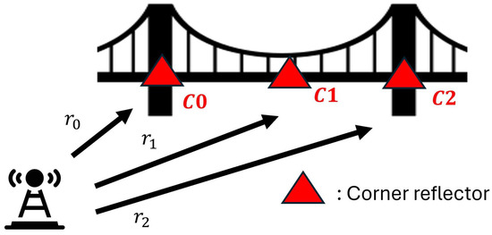
Figure 1.
Scenario of interest.
2.2. The Problem
Cars, trucks, and mopeds are expected to produce an interference on the measurement corner signal, corrupting the measurement. Here, those are referred to as dynamic clutter. Depending on the dynamic clutter radial velocity and the Pulse Repetition Frequency (PRF), the interference on the corner signal phase can be filtered out using a low-pass filter. However, when the dynamic clutter is so fast that its Doppler signature overlaps with the 0 Hz component, a standard low-pass filter is not a viable option anymore. Since the corner displacement information is expected to be in a neighborhood of the 0 Hz component, an excessively wide filter has no effect, while an excessively narrow filter deletes the corner displacement information and also preserves a portion of the dynamic clutter interference. Another way to address this problem is by using a staggered PRF method, which consists in employing a variable PRF so that the dynamic clutter response does not alias around 0 Hz. In such cases, the dynamic clutter Doppler response can be estimated and removed [19,20,21,22]. However, these algorithms cannot be applied in our operational scenario. The proposed work is meant to harvest sensing capability over an already deployed and PRF-fixed system. The worst case scenario is tackled when the dynamic clutter Doppler centroid falls exactly at the PRF. Thus, the critical dynamic clutter radial velocity can be written as [23]
For instance, in our use case scenario, the signal wavelength is 6 cm; using a high PRF, e.g., of 1 kHz, the radial velocity that overlaps with the 0 Hz Doppler component is 110 kmph. On the other hand, when the PRF has lower values, as, for instance, 400 Hz, a low-pass filter is not a viable option. Indeed, to make the dynamic clutter Doppler signature alias and fall over the 0 Hz component, the clutter radial velocity measured by the radar should be in the order of 12.2 m/s, approximately 44 kmph.
In Figure 2, two cases are presented. In Figure 2a, the dynamic clutter is simulated as a point scatterer moving at m/s, and the signal is acquired with two different PRFs: 1 kHz in Figure 2a and 400 Hz in Figure 2b. It is evident that in the scenario shown in Figure 2a, a low-pass filter is sufficient to suppress the dynamic clutter contribution. Conversely, in Figure 2b, the clutter moves at the system’s critical radial velocity, making a low-pass filtering approach ineffective.
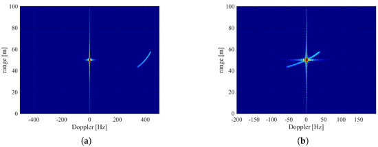
Figure 2.
Here, two different range-Doppler images are presented. (a) Simulated with 1 kHz PRF; (b) simulated with 400 Hz PRF. In the latter case, a low-pass filter is not a viable option to remove the dynamic clutter contribute.
3. Signal Model
The considered system is made up of a single channel working under the monostatic assumption, i.e., with transmitter and receiver co-located. The transmitted signal is a chirp at 5 GHz using 100 MHz of bandwidth. After the range compression at the receiver, the signal can be modeled as [23]
where r is the range axis, measuring the distances between the sensor and the scene, the variable records the slow time, whose spacing is determined by the Pulse Repetition Frequency (PRF). In Equation (2), represents the amplitude and phase scaling factor. The term is the distance between the target and the sensor at the slow-time , and is the transmitted signal wavelength. The term is the range resolution [23], and it has the form of
From the phase term in Equation (2), it is possible to read the displacement of a target inside a resolution cell [24]. Indeed, the displacement retrieved from the signal phase can be written as
where is the displacement of a target assuming that there is no range migration, i.e., the target does not move enough to change the resolution cell.
4. Image Plane Technique
Here, a method for eliminating clutter interference in cases of low Pulse Repetition Frequency (PRF) is proposed, leveraging radar imaging techniques. First, a brief description of the algorithm is provided, followed by an explanation of the imaging technique. Then, the effect of this technique on the focused signal is analyzed. Subsequently, the dynamic clutter suppression and defocusing procedures are presented. Finally, the computational complexity of the algorithm is addressed.
4.1. Rationale and Algorithm Description
This paper presents a solution to remove dynamic clutter interference when the dynamic clutter’s radial velocity causes its Doppler to alias and overlap with the 0 Hz component, thus making the use of a standard low-pass filter impossible. The main challenges addressed here concern dynamic clutter focusing, detection, and suppression. The first is achieved by estimating the dynamic clutter motion parameters and then performing SAR imaging, attributing the estimated movement to the antenna. This allows the projection of data into a spatial domain, the image plane, where the dynamic clutter is more compressed than the signal backscattered by the infrastructure. The focusing procedure and detection are addressed by using a 0 Hz notched version of the data. The detection step aims to establish an area to be removed. The suppression problem is tackled by thresholding the dynamic clutter portion and then by zero-forcing it. For clarity, one final step is required: the image should be transformed back from the image plane to the data domain in order to evaluate the measurement. The block diagram of our processing is shown in Figure 3.

Figure 3.
Processing block diagram.
4.2. Dynamic Clutter Imagery
The dynamic clutter is focused using Time Domain Backprojection (TDBP) [23]. This method involves the coherent summation of the pulses acquired by the radar, projected into the image plane, i.e., an area of interest, as
where is the image plane, is the focused image, is the distance between the radar and the image plane at the slow-time . Typically, in radar or Synthetic Aperture Radar (SAR) imaging, an array or prior knowledge on the platform motion is required. In our case, however, a single-channel system with a stationary antenna is considered. Therefore, the motion of the dynamic clutter is assigned to the antenna itself before focusing, thus faking a motion of the antenna as if it were a standard SAR platform. By doing so, the dynamic clutter is maximally compressed in the image plane, since the image is focused using a set of parameters that explains the dynamic clutter motion law by assigning to the antenna a linear trajectory. The estimation of the dynamic clutter motion parameters is tackled later in this section.
4.3. Static Signal Focusing
The static signal component, that is, the received signal backscattered by the still components of the scenario, is focused using the same parameters as the dynamic clutter. First, a remark should be made. Since a single-channel system is considered, the recorded data do not have direction of arrival (DoA) sensitivity. In the focused image, once is fixed to 0 and to the corresponding constant for the moving target to be focused, every angle corresponds to a different Doppler frequency as
where the squint angl and is the along-track velocity, the one used for focusing. So, taking this into account, the static targets appear at boresight of the synthetic antenna aperture.
4.4. Azimuth Ambiguities
If the data are acquired with a PRF such that the dynamic clutter spectrum overlaps with the 0 Hz component, the dynamic clutter Doppler centroid is considered to be the PRF, thus its radial velocity is estimated using Equation (1). This procedure leads to some azimuth ambiguities in the focused image [25,26]. This phenomenon influences both the dynamic clutter and the static signal. Indeed, the direction azimuth ambiguit appears at can be written as
where is the direction at which the ambiguity appears and is the along-track velocity, the one used for focusing. In Equation (7), just the first ambiguity is considered. Since the dynamic clutter results more compressed in its actual position rather than in its ambiguity, it is easier to be detected and removed. Therefore, a neighborhood of the dynamic clutter position is considered for our processing.
4.5. Dynamic Clutter Suppression
The dynamic clutter suppression technique follows a three-step procedure. First, the dynamic clutter must be detected and isolated in the focused image. This can be achieved by notching the static component in the range-compressed data domain, followed by the application of the focusing procedure. Second, a threshold is applied to the dynamic clutter image. Finally, the thresholded dynamic clutter contribution is removed from the image. This involves a coherent subtraction between the corrupted image and the thresholded one. The workflow of this procedure is shown in Figure 4.
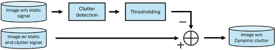
Figure 4.
Dynamic clutter suppression workflow.
A brief comment is necessary before proceeding. Notching the 0 Hz component may act as a high-pass filter. Therefore, a narrow filter should be applied to suppress only the 0 Hz component, without affecting the bandwidth of the superimposed dynamic clutter. Furthermore, the thresholding procedure must be carefully tuned. A threshold set too low may include some corner information, thereby eliminating both the clutter and the desired corner movement signals. Conversely, a threshold set too high may be insufficient to suppress the dynamic clutter interference. The algorithm leverages the TDBP to achieve maximal compression of the dynamic clutter signal, whereas the static signal exhibits a broader profile. Consequently, the dynamic clutter signal is expected to exhibit a greater amplitude than the static signal, most likely exceeding the chosen threshold. In the present study, the threshold was defined as the 99.8th percentile of the values below the peak of the dynamic clutter.
4.6. Defocusing
Now that the dynamic clutter contribution is canceled from the image, one last step is required. More precisely, the data should be brought from the image domain to the range compressed domain. This operation is focusing inverse operation that is called in Synthetic aperture radar processing defocusing operation. It consists in reconstructing the range compressed matrix associated with a SAR image. This is achieved by collecting and summing all the contributes in the image at the same distance with respect to a given point in the used trajectory. More formally, given an image , its reconstructed range compressed matrix can be reconstructed as
where is the complex value pixel of at the coordinate , and is the distance between the image plane and the platform trajectory at the slowtime . In our case, the considered trajectory is the one attributed to the antenna. Then, the corner displacement can be retrieved using Equation (4).
4.7. Retrieval of Motion Parameters
To estimate the clutter motion to be attributed to the antenna, some assumptions need to be considered. The radial velocity is modeled as the scalar product between the velocity of the target and the versor of the line of sight as
where is the squint angle and is the scalar product operator. A graphical representation can be found in Figure 5.
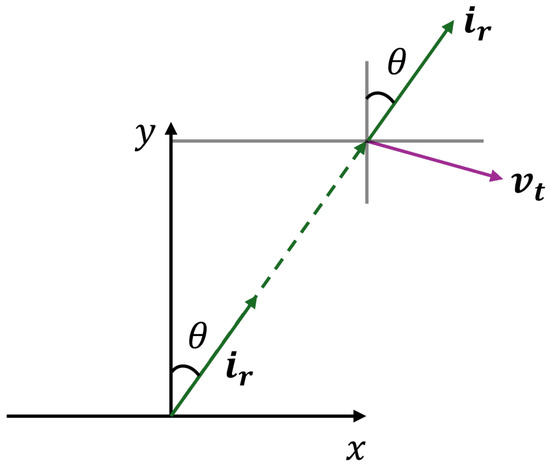
Figure 5.
Graphical representation of the radial velocity.
The radar records a curve as
where are the central positions of the clutter trajectory, and are the velocities along the x and y directions. In Equation (10), the radar position is assumed to be in the origin of the reference system. Since our system is made up by one antenna, a precise retrieval of the clutter motion parameters is not possible. Therefore, a set of three parameters is sought such that
In other words, given a clutter signature law , this law is explained as a function of three parameters instead of four, arbitrarily setting to zero. In practice, a linear trajectory and a coordinate pair are needed, such that the curve recorded by the radar can be explained by a linear motion. The estimation procedure is carried on using an exhaustive search on the parameter space. More precisely, from the range-Doppler map, the range-Doppler centroid coordinates are extracted. is the centroid range coordinate, while in our case coincides with the PRF. The Doppler coordinate can be transformed into the radial velocity using Equation (1). At this point, the only parameter needed to focus the dynamic clutter is an along-track velocity. It can be estimated using Equation (9), considering equal to 0 and by trying a battery of possible focusing angles . So, an exhaustive search of a set of possible angles is performed to search for the optimal focusing angle. First, the dynamic clutter spatial centroid is computed as
where is the dynamic clutter range at and is the focusing angle. Then, a neighborhood of the dynamic clutter is focused for each possible angle, and finally, the angle giving the highest peak in the focused image is chosen. The along-track velocity used for focusing can be retrieved from Equation (6). It is trivial a variation in the focusing angle also produces a variation in . The above procedure is applied to the 0 Hz notched aliased dynamic clutter data.
4.8. Computational Complexity Analysis
The proposed algorithm relies on Time-Domain Back-Projection (TDBP) for SAR image formation. The computational complexity of generating a single complex image scales linearly with the number of slow-time samples and with the size of the focused image [27], namely
where denotes the focused image size. In (13), the cost of the interpolation kernel is neglected. The algorithm performs an exhaustive search over a discrete set of focusing angles, i.e., one complex image is produced for each candidate angle. More precisely,
where is the cardinality of the focusing-angle set. Once the optimal focusing angle is identified, the algorithm generates a SAR image of the entire scene at the computational cost given in (13). Subsequently, after thresholding and subtraction, the algorithm applies a defocusing operation. The defocusing step consists of collecting and summing all contributions at the same distance with respect to a given point along the trajectory, namely
where is the number of range samples. Therefore, the total computational complexity can be computed as
5. Numerical Simulation
In this section, a simulation is proposed in order to provide a numerical evaluation for our algorithm. The proposed simulation consists in a sinusoidal corner movement of amplitude 2 mm and period s. The simulation PRFs are 1 kHz and 400 Hz. The former is meant to provide the dynamic clutter focused images without azimuth ambiguities at its expected velocity; the latter is used to perform the actual test of the algorithm. A point scatterer that represents the dynamic clutter impinges on the movement of the corners. The dynamic clutter moves at the critical radial velocity of the system, 400 Hz. The effect on the measured phase can be found in Figure 6. The simulation carrier frequency is 5 GHz and the associated bandwidth is 60 MHz. In Figure 6, the corner displacement corrupted by the dynamic clutter shows a pattern different from the actual corner displacement. As said in Section 4, the imagery procedure needs to be performed. First, a battery of possible angles and therefore velocities is tested. The proposed focuser returns as selected angle the one compressing more the dynamic clutter. The selection is made among the focused dynamic clutter peaks. In Figure 7, the relationship between peak power and focusing angle is illustrated. Here, first the 1 kHz image is reported. In Figure 8, the scene is focused with the estimated parameters. The dynamic clutter is highlighted in green. It results in a focused point impulse response of a SAR imaging system. The static signal component is highlighted in red in Figure 8. The static signal component is coherently focused in front of the trajectory associated to the antenna. Now, the 400 Hz simulation is tackled. The dynamic clutter is ocused using a notched version of the data, as in Section 4.5, returning the same focusing angle and clutter as the 1 kHz data. The resulting image is referred as dynamic clutter image. Then the 400 Hz data are focused. For the sake of completeness, the effect of the azimuth ambiguities is proposed in Figure 9. The static signal ambiguity and the real dynamic clutter signal are highlighted in green; the two are superimposed in the image plane. This also happens for the dynamic clutter ambiguity and the real static signal, in red. It can be noticed that the dynamic clutter results more compressed in its actual position within respect to its replica. Also, it can be noticed that the static signal ambiguity carries the same corner phase information of its counterpart. For these reasons, for the purpose of our processing scheme, a neighborhood of the dynamic clutter actual position and static signal ambiguity is considered. Then, the dynamic clutter image is thresholded and then subtracted to the 400 Hz image. The result of this procedure can be found in Figure 10. This is a non-linear operation due to the thresholding operation. The subtraction can be performed coherently, without incurring in side-lobes or grating-lobes. This is because the spectral support of the dynamic clutter is the same in both images. This is a trivial consequence of the fundamental theorem of diffraction tomography [28,29]. Then the resulting image is defocused using the same parameters used for focusing. A comparison between the ideal corner displacement, the corrupted one, and the one retrieved after the suppression procedure can be found in Figure 11. In Figure 11, the dynamic clutter interference on the corner displacement measurement is canceled. Numerically, the mean error between the ideal displacement and the corrupted one is mm, and its standard deviation is mm. On the contrary, the mean error between the ideal displacement and the one retrieved after the canceling procedure is mm, and its standard deviation is mm.
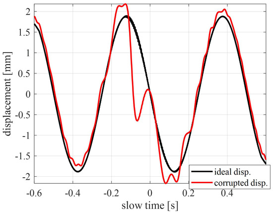
Figure 6.
Corner displacement retrieved at the receiver. In red, a simulated corner displacement is reported in a 400 Hz scenario. In black, the ideal displacement is reported.
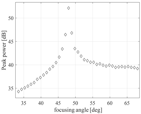
Figure 7.
Here, the relationship between the focusing angle and the peak power is illustrated.
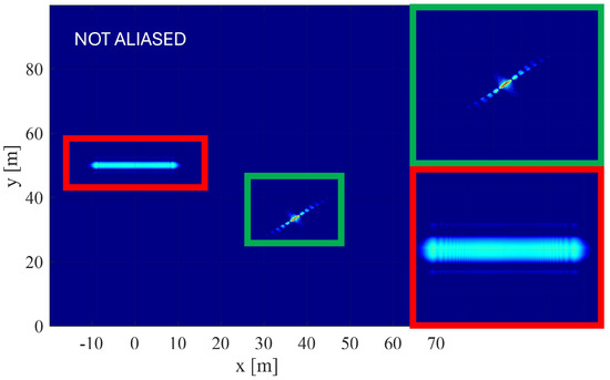
Figure 8.
Here, a 1 kHz simulated dat are focused using the dynamic clutter parameters. The static signal component is highlighted in red, while the dynamic clutter is displayed in green.
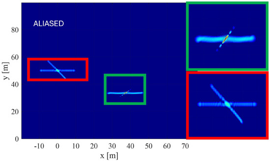
Figure 9.
Here, the focused scene of a data simulated using a 400 Hz as PRF is presented. The dynamic clutter was simulated using the system critical radial velocity.
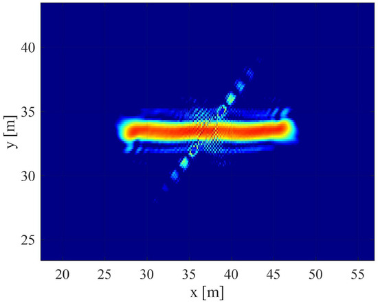
Figure 10.
Here, the dynamic clutter is canceled using the procedure described in Section 4.5. The majority of the dynamic clutter contribution is removed.
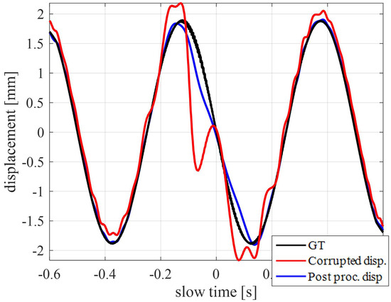
Figure 11.
Here, a comparison between the corner displacement is reported. In black, the displacement retrieved form the 1 kHz simulation is reported; in red, the one retrieved from the 400 Hz simulation is reported, and in blue, the one retrieved after the canceling procedure is shown.
6. Real Data Results
In this section, some results from a real data experiment conducted by Huawei Technologies are presented. In this experiment, the carrier frequency was set at 5 GHz, with a bandwidth of 60 MHz and a pulse repetition frequency (PRF) of 400 Hz. Here, two case studies are proposed. To establish the ground truth for algorithm validation in the absence of external sensor measurements, we adopt the following procedure. First, a case is selected in which dynamic clutter interference can be removed using a Doppler low-pass filter. This displacement of the corner reflector is then taken as the ground truth for the experiment. Subsequently, dynamic clutter is artificially aliased in order to recreate a scenario suitable for testing our algorithm. The resulting dataset is regarded as corrupted data from which the corner displacement must be retrieved. A visual representation of the scenario can be found in Figure 12.
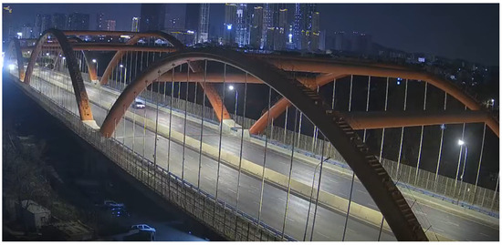
Figure 12.
Optical reference for the monitored infrastructure.
Also, a geometrical representation of the scenario can be found in Figure 13.
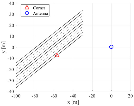
Figure 13.
Geometrical representation of the infrastructure scenario.
6.1. First Case Study
The optical reference for the first case study is proposed in Figure 14. It consists of a bus that passes throughes through the bridge at a speed of 37 kmph.
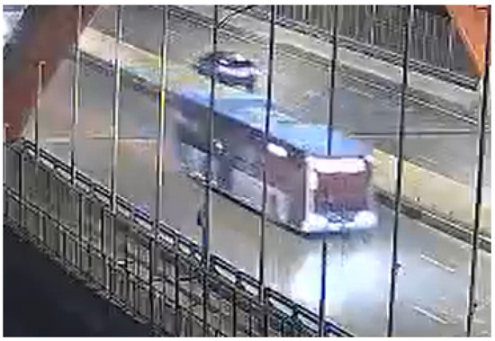
Figure 14.
Here, the dynamic clutter optical reference is shown.
The data are undersampled to make the dynamic clutter Doppler signature fall over the 0 Hz Doppler component. The ideal corner displacement can be found in Figure 15, depicted in black.
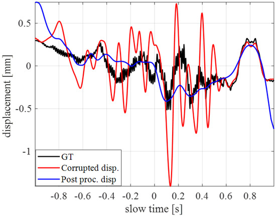
Figure 15.
Here, a comparison between the corner displacements is proposed. In black is the ground truth (GT), in red is the corner displacement corrupted by the dynamic clutter interference, in blue is the displacement retrieved after the coherent subtraction is proposed.
The scene is processed using the procedure described in Section 4. First, the dynamic clutter is focused by an exhaustive search on a set of possible squint angle. A neighborhood of the dynamic clutter is focused at each step, using the relationship in Equation (12).
The focusing angle that maximizes the dynamic clutter amplitude is degrees. Also, in Figure 16a, the shape of the dynamic clutter can be recovered. The full scene can be found in Figure 17. Here, the static signal component is focused in front of the fake trajectory given to the antenna, while the dynamic clutter is focused at its squint angle. The trajectory given to the antenna to deliver the proposed image is approximately 23 m long, providing an azimuth resolution of m at the dynamic clutter coordinate. As said above, the data are undersampled to make the dynamic clutter Doppler contribute fall over the 0 Hz component. The corner displacement retrieved at this point can be found in Figure 15 in red. Successively, a notched version of the undersampled data is focused for dynamic clutter detection purposes and proposed in Figure 16a. The resulting focusing parameters are consistent with the previous step. Then, the resulting image is thresholded at the 99th percentile. The resultant portion is proposed in Figure 16b. A neighborhood of the dynamic clutter and the static signal azimuth ambiguity is focused and proposed in Figure 16c. Finally, the image in Figure 16d is defocused, and the corner displacement can be retrieved. The corner displacement retrieved after this procedure is proposed in Figure 15, in blue. In Figure 15, the displacement recovered after the filtering procedure (blue line) follows almost the same pattern as the ground truth (black line). The root mean square error (RMSE) between the corrupted displacement (red line) and the ground truth (black line) is about mm. On the contrary, the displacement retrieved after the cancellation procedure (blue line) and the ground truth (black line) is about mm.
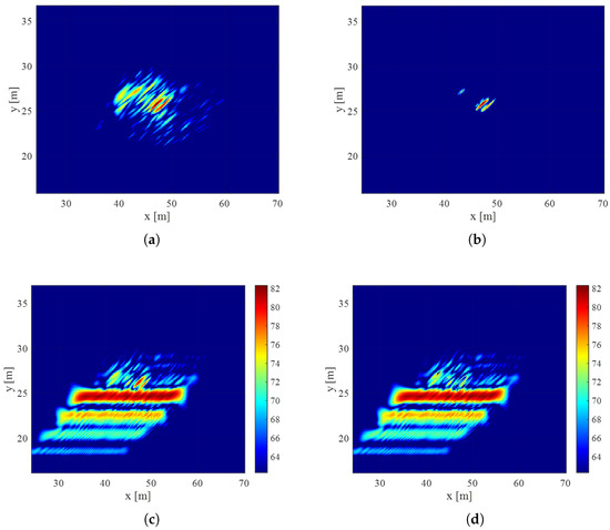
Figure 16.
Here, different stages of the image plane technique are proposed. In (a), the dynamic clutter image is proposed. In (b), a thresholded version of the dynamic clutter image is proposed. In (c), the focused undersampled data are proposed. The dynamic clutter is shown to be superimposed to the static signal replica. In (d), the dynamic clutter is coherently subtracted. The above images are in dB.
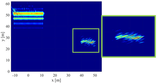
Figure 17.
Here, the dynamic clutter contribute and the clutter signal are not superimposed, since the dynamic clutter is not fast enough to cause aliasing in Doppler.
6.2. Second Case Study
The optical reference for the first case study is proposed in Figure 18. It consists in a truck passing on the bridge at a speed of 33 kmph.

Figure 18.
Here, the dynamic clutter optical reference is shown.
The data are undersampled to make the dynamic clutter Doppler signature fall over the 0 Hz Doppler component. The ideal corner displacement can be found in Figure 19, depicted in black. The scene is processed using the procedure described in Section 4. First, the dynamic clutter is focused by an exhaustive search on a set of possible squint angle. A neighborhood of the dynamic clutter is focused at each step, using the relationship in Equation (12). The focusing angle that maximizes the dynamic clutter amplitude is degrees. Also, in Figure 20a, the shape of the dynamic clutter can be recovered. The full scene can be found in Figure 21. Here, the static signal component is focused in front of the fake trajectory given to the antenna, while the dynamic clutter is focused at its squint angle. The trajectory given to the antenna to deliver the proposed image is approximately m long, providing an azimuth resolution of m at the dynamic clutter coordinate.
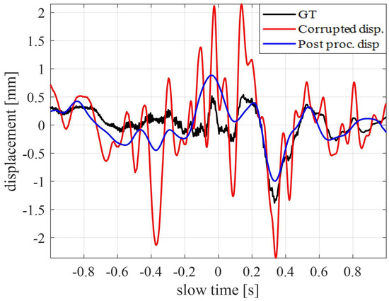
Figure 19.
Here, a comparison between the corner displacements is proposed. In black is the ground truth (GT), in red is the corner displacement corrupted by the dynamic clutter interference, in blue is the displacement retrieved after the coherent subtraction is proposed.
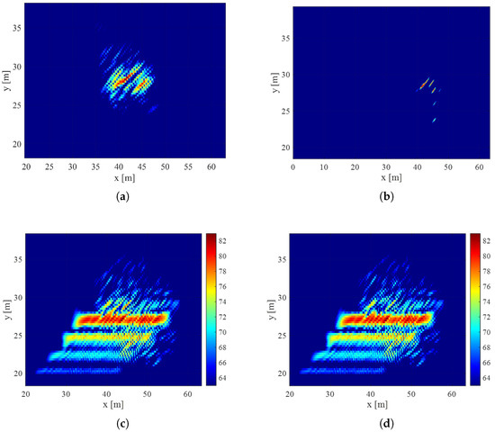
Figure 20.
Here, different stages of the image plane technique are proposed. In (a), the dynamic clutter image is proposed. In (b), a thresholded version of the dynamic clutter image is proposed. In (c), the focused undersampled data are proposed. The dynamic clutter is shown to be superimposed to the static signal replica. In (d), the dynamic clutter is coherently subtracted. The above images are in dB.
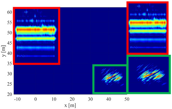
Figure 21.
Here, the dynamic clutter contribute and the clutter signal are not superimposed, since the dynamic clutter is not fast enough to cause aliasing in Doppler.
As said above, the data are undersampled to make the dynamic clutter Doppler contribute fall over the 0 Hz component. The corner displacement retrieved at this point can be found in Figure 19 in red. Successively, a notched version of the undersampled data are focused for dynamic clutter detection purposed and are proposed in Figure 20a. The resulting focusing parameters are consistent with the previous step. Then, the resulting image is thresholded at the 99th percentile. The resultion portion is proposed in Figure 20b. A neighborhood of the dynamic clutter and the static signal azimuth ambiguity is focused and proposed in Figure 20c. Then a thresholded version of the dynamic clutter image is coherently subtracted to the previous one, as described in Section 4.5. The threshold is selected as the 99th percentile of the dynamic clutter peak. The result of the coherent subtraction is provided in Figure 20d. Finally, the image in Figure 20d is defocused, and the corner displacement can be retrieved. The corner displacement retrieved after this procedure is proposed in Figure 19, in blue. In Figure 19, the displacement recovered after the filtering procedure (blue line) follows almost the same pattern as the ground truth (black line). The RMSE between the the corrupted displacement (red line) and the ground truth (black line) is about mm. On the contrary, the displacement retrieved after the cancellation procedure (blue line) and the ground truth (black line) is about mm.
6.3. A Fortunate By-Product
As a by-product of this technique, there is the capability to perform electromagnetic imagery of different dynamic clutters. The procedure is the one described in Section 4. The only exception is made by the dynamic clutter Doppler centroid. Indeed, the selected Doppler centroid may not coincide with the PRF. Some examples are reported in Figure 22. Using the proposed focusing technique, the shape of the dynamic clutters can be recovered.
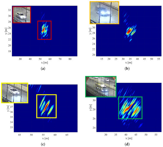
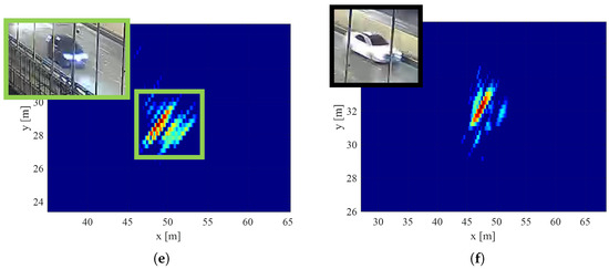
Figure 22.
Here, an example of the dynamic clutter imagery capability is proposed. (a) shows a car whose radial velocity is 64 kmph. (b) presents a bigger vehicle, with a recorded radial velocity of 56 kmph. (c) displays a car moving at a radial velocity of 50 kmph. In addition, (d) depicts a truck whose radial velocity reaches 33 kmph. Finally, (e,f) show two vehicles moving at a radial velocity of 58 kmph and 60 kmph, respectively.
7. Conclusions
In this work, a radar imagery-based signal processing technique to eliminate dynamic clutter interference in Structural Health Monitoring (SHM) is proposed. This can be considered an application of joint communication and sensing within telecommunication infrastructure, leveraging already deployed sub-6G gNodeB base stations as a ground-based radar. The proposed technique is applicable even in the presence of dynamic clutter, where its Doppler contribution aliases and overlaps with the 0 Hz component. In such cases, a standard low-pass filter is not a viable option. Indeed, a low-pass filter that is too shallow preserves the dynamic clutter contribution, while one that is too narrow eliminates the displacement information and still preserves the dynamic clutter.
The proposed approach leverages Time Domain Backprojection (TDBP) to transfer the dynamic clutter from the data domain to an image plane in which it is maximally compressed, making it easier to remove than in the range-Doppler domain. First, an estimation of the dynamic clutter motion parameters is performed through an exhaustive search over a set of possible velocities. Due to the high radial velocity of the clutter, the focused images exhibit azimuth ambiguities, which are exploited to retrieve the corner displacement. Dynamic clutter detection is carried out by focusing a notched version of the range-compressed data. Dynamic clutter cancellation is then achieved through coherent subtraction. Subsequently, the resulting image is defocused to retrieve the displacement.
A numerical simulation is conducted to evaluate the effectiveness of the method, showing consistency with the ideal displacement. Additionally, real case studies are presented. The experimental campaign is performed by Huawei Technologies in the C-band. The validation shows consistency with the ground truth, providing improvements in the mean error and its variance compared to the corrupted displacement. The algorithm threshold must be carefully calibrated on a case-by-case basis. The selection of the threshold is highly dependent on the experimental geometry and system parameters. In an operational scenario, the validation procedure proposed herein can be employed to calibrate the threshold prior to deployment. The algorithm is evaluated using experimental data and demonstrates the capability to effectively remove the majority of phase errors caused by clutter from larger vehicles like trucks and buses. In contrast, smaller vehicles generate only minimal errors; in such cases, the algorithm shows little to no noticeable enhancement.
As a by-product of this algorithm, radar imagery of moving vehicles can also be performed.
Based on the authors’ experience, the possibility of two vehicles aliasing together is very unlikely, as this would require them to have the same speed and to occupy the same resolution cell at the same time. In such a case, the algorithm would simply treat them as an extended target. Most targets can be effectively removed using a Doppler low-pass filter, while the proposed algorithm is intended for those cases in which such filtering is not sufficient. Due to the high computational cost of this algorithm, real-time implementation is currently not feasible. Future research could explore GPU-based implementations and a factorized processor; however, this is beyond the scope of the present article and is left for future work.
Author Contributions
Conceptualization, M.G.P. and S.T.; methodology, M.G.P. and S.T.; software, M.G.P.; validation, M.G.P., S.T. and M.M.; formal analysis, M.G.P. and S.T.; investigation, M.G.P.; resources, S.T., D.B. and S.D.; data curation, M.G.P. and S.T.; writing—original draft preparation, M.G.P.; writing—review and editing, M.G.P., S.T., D.B., M.M. and S.D.; visualization, M.G.P.; supervision, S.T.; project administration, S.T. and D.B.; funding acquisition, S.T. All authors have read and agreed to the published version of the manuscript.
Funding
This work was partially supported by the European Union—Next Generation EU under the Italian National Recovery and Resilience Plan (NRRP), Mission 4, Component 2, Investment 1.3, CUP D43C22003080001, partnership on “Telecommunications of the Future” (PE00000001-program “RESTART”).
Informed Consent Statement
Not applicable.
Data Availability Statement
No dataset is publicly available.
Acknowledgments
This work was partially supported by the European Union—Next Generation EU under the Italian National Recovery and Resilience Plan (NRRP), Mission 4, Component 2, Investment 1.3, CUP D43C22003080001, partnership on “Telecommunications of the Future” (PE00000001-program “RESTART”). This work has been carried out in the context of the activities of the Joint Lab by Huawei Technologies Italia and Politecnico di Milano.
Conflicts of Interest
Damiano Badini and Sergi Duque are currently Huawei Technologies employees. Their company approved the publication of the paper with them as co-authors.
Abbreviations
The following abbreviations are used in this manuscript:
| SHM | Structural Health Monitoring |
| TDBP | Time Domain Backprojection |
| SAR | Synthetic Aperture Radar |
| InSAR | Synthetic Aperture Radar Interferometry |
| GBRI | Ground-Based Radar Interferometry |
| JCAS | Joint Communication and Sensing |
| PRF | Pulse Repetition Frequency |
| DoA | Direction of Arrival |
| SCR | Signal-to-Clutter Ratio |
| RMSE | Root Mean Square Error |
References
- Dong, Y.; Song, R.; Liu, H. Bridges Structural Health Monitoring and Deterioration Detection-Synthesis of Knowledge and Technology; Technical Report; University of Alaska Fairbanks: Fairbanks, AK, USA, 2010. [Google Scholar]
- Wenzel, H. Health Monitoring of Bridges; John Wiley & Sons: Hoboken, NJ, USA, 2008. [Google Scholar]
- Harms, T.; Sedigh, S.; Bastianini, F. Structural health monitoring of bridges using wireless sensor networks. IEEE Instrum. Meas. Mag. 2010, 13, 14–18. [Google Scholar] [CrossRef]
- Ferretti, A.; Savio, G.; Barzaghi, R.; Borghi, A.; Musazzi, S.; Novali, F.; Prati, C.; Rocca, F. Submillimeter accuracy of InSAR time series: Experimental validation. IEEE Trans. Geosci. Remote Sens. 2007, 45, 1142–1153. [Google Scholar] [CrossRef]
- Cusson, D.; Rossi, C.; Ozkan, I. Early warning system for the detection of unexpected bridge displacements from radar satellite data. J. Civ. Struct. Health Monit. 2021, 11, 189–204. [Google Scholar] [CrossRef]
- Gagliardi, V.; Tosti, F.; Bianchini Ciampoli, L.; Battagliere, M.L.; D’Amato, L.; Alani, A.M.; Benedetto, A. Satellite remote sensing and non-destructive testing methods for transport infrastructure monitoring: Advances, challenges and perspectives. Remote Sens. 2023, 15, 418. [Google Scholar] [CrossRef]
- Talledo, D.A.; Miano, A.; Bonano, M.; Di Carlo, F.; Lanari, R.; Manunta, M.; Meda, A.; Mele, A.; Prota, A.; Saetta, A.; et al. Satellite radar interferometry: Potential and limitations for structural assessment and monitoring. J. Build. Eng. 2022, 46, 103756. [Google Scholar] [CrossRef]
- Monti-Guarnieri, A.; Falcone, P.; d’Aria, D.; Giunta, G. 3D vibration estimation from ground-based radar. Remote Sens. 2018, 10, 1670. [Google Scholar] [CrossRef]
- Michel, C.; Keller, S. Advancing ground-based radar processing for bridge infrastructure monitoring. Sensors 2021, 21, 2172. [Google Scholar] [CrossRef] [PubMed]
- Luzi, G.; Pieraccini, M.; Mecatti, D.; Noferini, L.; Guidi, G.; Moia, F.; Atzeni, C. Ground-based radar interferometry for landslides monitoring: Atmospheric and instrumental decorrelation sources on experimental data. IEEE Trans. Geosci. Remote Sens. 2004, 42, 2454–2466. [Google Scholar] [CrossRef]
- Diaferio, M.; Fraddosio, A.; Piccioni, M.D.; Castellano, A.; Mangialardi, L.; Soria, L. Some issues in the structural health monitoring of a railway viaduct by ground based radar interferometry. In Proceedings of the 2017 IEEE Workshop on Environmental, Energy, and Structural Monitoring Systems (EESMS), Milan, Italy, 24–25 July 2017; pp. 1–6. [Google Scholar]
- Zhang, J.A.; Liu, F.; Masouros, C.; Heath, R.W.; Feng, Z.; Zheng, L.; Petropulu, A. An overview of signal processing techniques for joint communication and radar sensing. IEEE J. Sel. Top. Signal Process. 2021, 15, 1295–1315. [Google Scholar] [CrossRef]
- Liu, A.; Huang, Z.; Li, M.; Wan, Y.; Li, W.; Han, T.X.; Liu, C.; Du, R.; Tan, D.K.P.; Lu, J.; et al. A survey on fundamental limits of integrated sensing and communication. IEEE Commun. Surv. Tutor. 2022, 24, 994–1034. [Google Scholar] [CrossRef]
- Wei, Z.; Qu, H.; Wang, Y.; Yuan, X.; Wu, H.; Du, Y.; Han, K.; Zhang, N.; Feng, Z. Integrated sensing and communication signals toward 5G-A and 6G: A survey. IEEE Internet Things J. 2023, 10, 11068–11092. [Google Scholar] [CrossRef]
- González-Prelcic, N.; Tagliaferri, D.; Keskin, M.F.; Wymeersch, H.; Song, L. Six Integration Avenues for ISAC In 6G and Beyond: A Forward-Looking Vision. IEEE Veh. Technol. Mag. 2025, 20, 18–39. [Google Scholar] [CrossRef]
- Tan, D.K.P.; He, J.; Li, Y.; Bayesteh, A.; Chen, Y.; Zhu, P.; Tong, W. Integrated sensing and communication in 6G: Motivations, use cases, requirements, challenges and future directions. In Proceedings of the 2021 1st IEEE International Online Symposium on Joint Communications & Sensing (JC&S), Dresden, Germany, 23–24 February 2021; pp. 1–6. [Google Scholar]
- Santi, F.; Pisciottano, I.; Pastina, D.; Cristallini, D. Multi-angle DVB-S based passive ISAR sensitivity to target motion estimation errors. In Proceedings of the 2023 IEEE Radar Conference (RadarConf23), San Antonio, TX, USA, 1–5 May 2023; pp. 1–6. [Google Scholar]
- Colone, F.; Filippini, F.; Di Seglio, M.; Chetty, K. On the use of reciprocal filter against WiFi packets for passive radar. IEEE Trans. Aerosp. Electron. Syst. 2021, 58, 2746–2761. [Google Scholar] [CrossRef]
- Pieraccini, M.; Miccinesi, L. Ground-based radar interferometry: A bibliographic review. Remote Sens. 2019, 11, 1029. [Google Scholar] [CrossRef]
- Miao, C.; Zhang, W.; Qin, Z.; Wu, W. Fast distance and velocity estimation in parameter agility radar using CM-CS-OMP and CM-MUSIC methods. Digit. Signal Process. 2025, 157, 104915. [Google Scholar] [CrossRef]
- Liu, Z.; Li, D.; Guo, H.; Wang, X. Research on Radar Clutter Suppression Method Based on Stagger MTI. J. Phys. Conf. Ser. 2023, 2625, 012031. [Google Scholar] [CrossRef]
- Ferrari, A.; Berenguer, C.; Alengrin, G. Doppler ambiguity resolution using multiple PRF. IEEE Trans. Aerosp. Electron. Syst. 2002, 33, 738–751. [Google Scholar] [CrossRef]
- Curlander, J.C.; McDonough, R.N. Synthetic Aperture Radar; Wiley: New York, NY, USA, 1991; Volume 11. [Google Scholar]
- Hanssen, R.F. Radar Interferometry: Data Interpretation and Error Analysis; Springer Science & Business Media: Berlin, Germany, 2001; Volume 2. [Google Scholar]
- Guarnieri, A.M. Adaptive removal of azimuth ambiguities in SAR images. IEEE Trans. Geosci. Remote Sens. 2005, 43, 625–633. [Google Scholar] [CrossRef]
- Moreira, A. Suppressing the azimuth ambiguities in synthetic aperture radar images. IEEE Trans. Geosci. Remote Sens. 1993, 31, 885–895. [Google Scholar] [CrossRef]
- Polisano, M.G.; Manzoni, M.; Tebaldini, S. Synthetic Aperture Radar Processing Using Flexible and Seamless Factorized Back-Projection. Remote Sens. 2025, 17, 1046. [Google Scholar] [CrossRef]
- Wu, R.S.; Toksöz, M.N. Diffraction tomography and multisource holography applied to seismic imaging. Geophysics 1987, 52, 11–25. [Google Scholar] [CrossRef]
- Polisano, M.G.; Manzoni, M.; Tebaldin, S.; Monti-Guarnieri, A.V.; Prati, C.M.; Russo, I. Automotive MIMO-SAR Imaging from Non-continuous Radar Acquisitions. In Proceedings of the 2023 Photonics & Electromagnetics Research Symposium (PIERS), Prague, Czech Republic, 3–6 July 2023; pp. 578–587. [Google Scholar]


Disclaimer/Publisher’s Note: The statements, opinions and data contained in all publications are solely those of the individual author(s) and contributor(s) and not of MDPI and/or the editor(s). MDPI and/or the editor(s) disclaim responsibility for any injury to people or property resulting from any ideas, methods, instructions or products referred to in the content. |
© 2025 by the authors. Licensee MDPI, Basel, Switzerland. This article is an open access article distributed under the terms and conditions of the Creative Commons Attribution (CC BY) license (https://creativecommons.org/licenses/by/4.0/).