Abstract
Registering light detection and ranging (LiDAR) data with optical camera images enhances spatial awareness in autonomous driving, robotics, and geographic information systems. The current challenges in this field involve aligning 2D-3D data acquired from sources with distinct coordinate systems, orientations, and resolutions. This paper introduces a new pipeline for camera–LiDAR post-registration to produce colorized point clouds. Utilizing deep learning-based matching between 2D spherical projection LiDAR feature layers and camera images, we can map 3D LiDAR coordinates to image grey values. Various LiDAR feature layers, including intensity, bearing angle, depth, and different weighted combinations, are used to find correspondence with camera images utilizing state-of-the-art deep learning matching algorithms, i.e., SuperGlue and LoFTR. Registration is achieved using collinearity equations and RANSAC to remove false matches. The pipeline’s accuracy is tested using survey-grade terrestrial datasets from the TX5 scanner, as well as datasets from a custom-made, low-cost mobile mapping system (MMS) named Simultaneous Localization And Mapping Multi-sensor roBOT (SLAMM-BOT) across diverse scenes, in which both outperformed their baseline solutions. SuperGlue performed best in high-feature scenes, whereas LoFTR performed best in low-feature or sparse data scenes. The LiDAR intensity layer had the strongest matches, but combining feature layers improved matching and reduced errors.
1. Introduction
Aligning LiDAR data with optical camera images is essential for improving spatial awareness in fields like autonomous driving, robotics, and geographic information systems [1]. However, aligning 3D point data with 2D images is challenging due to differences in coordinate systems, field of view, and how they are encoded and organized. Traditional registration methods often depend on explicit targets [2,3] and human intervention [4,5]. Recognizing these weaknesses, recent methods have transformed LiDAR data into 2D images to facilitate feature correspondences as an intermediate step to 2D–3D registration [6,7]. However, each of these methods only relies on a single feature of the LiDAR data, leaving a gap for increasing strong matching points utilizing the multi-feature capability. Furthermore, existing methods rely on similar projection models between 2D LiDAR and images [8], which leaves gaps in the projected 2D LiDAR data due to interpolation issues and results in less robust matching points.
Leahy and Jabari [9] registered georeferenced orthoimages with aerial LiDAR, combining intensity, elevation, and bearing angle LiDAR information with 2D feature layers. This approach was able to employ an affine transformation model for registration. However, when LiDAR data and camera images come from different projection models, and pre-registration is not available, as is typical in real-world applications, it becomes challenging to register such data, especially considering the different geometric imaging configurations. Terrestrial scene registration is more challenging than aerial registration due to factors such as occlusions, cross-projection models, varying scales, and the complexity of the environment.
We propose a new registration pipeline that uses 2D spherical LiDAR features as an intermediary to match the LiDAR point clouds with camera images. This approach allows the correspondence between spherical LiDAR features (in a spherical coordinate system) and 3D ground coordinates to effectively map spectral observations from camera images onto 3D points, resulting in colorized or multi-spectral point clouds when available. Since LiDAR provides range measurements, 2D spherical coordinates can be converted into XYZ ground coordinates. Consequently, the relationship between 2D RGB coordinates and 3D ground coordinates is established using collinearity equations.
Our method involves deep learning feature-based image matching algorithms, employing various combinations of feature layers through cross-modal matching to identify corresponding points between spherically projected LiDAR data and pre-calibrated camera images. To establish the 2D–3D registrations, we employ collinearity equations in conjunction with RANSAC [10] to minimize registration errors.
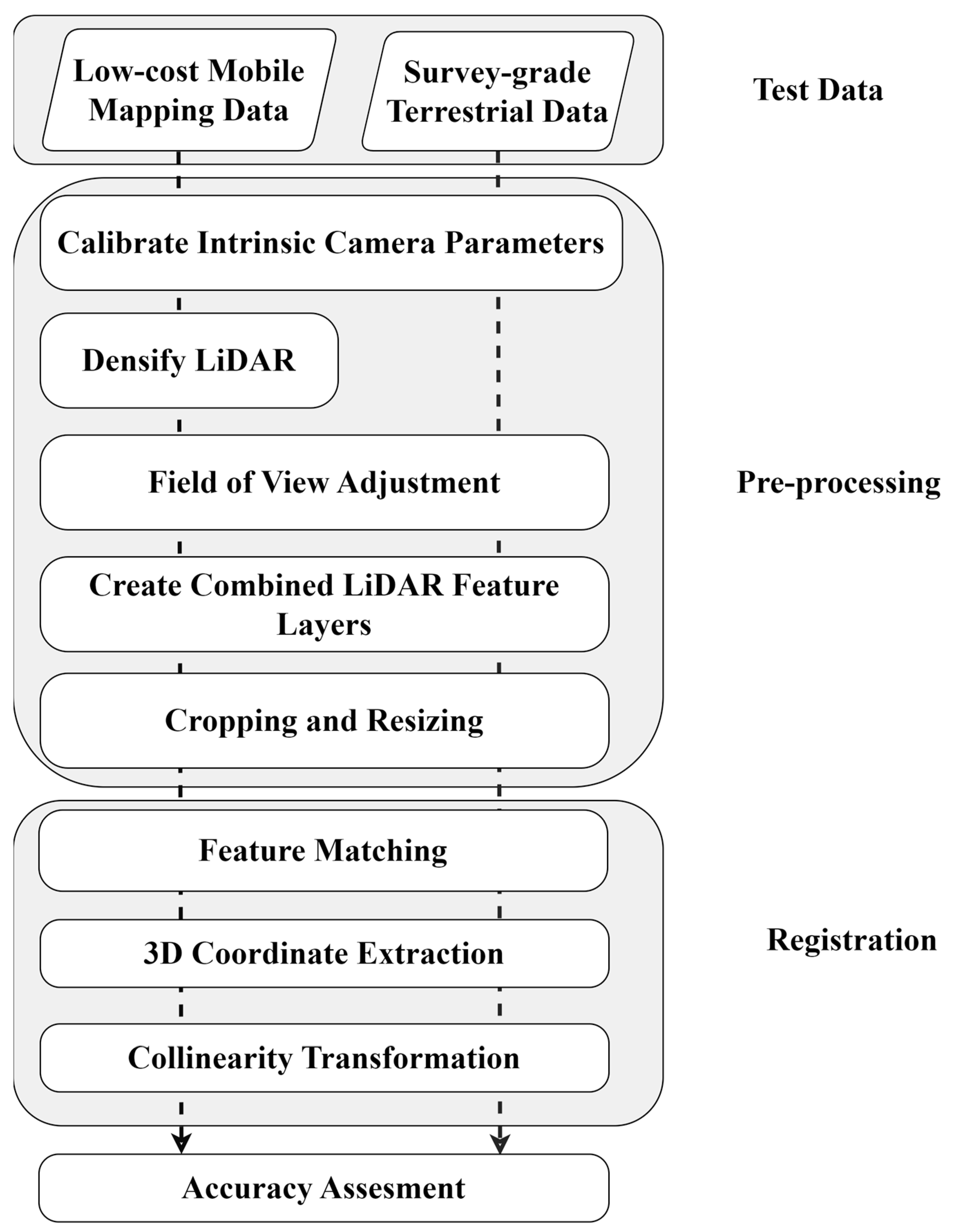
Figure 1 illustrates the methodology employed in this research. The process begins with the pre-calibration of cameras to determine interior orientation parameters. Subsequently, the LiDAR data were captured by SLAMM-BOT, which undergoes initial densification using SLAM techniques. Additionally, datasets captured from the TX5 scanner and SLAMM-BOT require initial preprocessing, including field of view (FOV) rotation, scaling, and cropping. To simplify the process, an initial low-accuracy registration between LiDAR and the camera can be applied, which can later be refined using our proposed method [11,12]. To ensure compatibility, the cross-modal data are adjusted to achieve a uniform field of view of the scene.

Figure 1.
General flowchart of the methodology.
There are several feature layers that can be included in this process. However, we focused on three of the most commonly cited LiDAR feature layers found in the literature: intensity, depth, and bearing angle attributes. We combined and weighted these layers for our analysis.
These layers are cropped and resized to align with the spatial resolution and dimensions of the optical image. Feature matching uses advanced algorithms such as SuperGlue and LoFTR to identify corresponding features across the cross-modal datasets. Next, the derived 3D ground coordinates are utilized to establish collinearity equations, facilitating the registration of LiDAR data with camera images. We test our approach using survey-grade terrestrial laser scanner (TX5), handheld cameras, and SLAMM-BOT data.
2. Related Works
LiDAR data offer 3D geometric representations and are conventionally processed and analyzed as point clouds. However, recent interest lies in representing LiDAR as a 2D image to establish more robust correspondences with camera images. For instance, Li and Li [13] focused on projecting LiDAR range data onto the horizontal image plane for MMS localization in sparse outdoor environments. Dong et al. [14] employed a cylindrical range image representation for tasks like neighbor search and down-sampling. Similarly, Liu et al. [15] experimented with dense laser scanners to generate bearing angle (BA) and fast optimal bearing angle (FOBA) images for outdoor scene segmentation. Park et al. [16] extended these techniques to indoor scenes, leveraging intensity data from industrial laser scanners for point cloud registration and geometric optimization.
Two-dimensional LiDAR representations for feature correspondence are helpful, but matching LiDAR’s features to an optical image requires advanced techniques due to their differing geometric and spectral characteristics. Traditional methods like SIFT [17] are commonly used for detecting and matching keypoints in camera images, by analyzing the pixel’s intensity, magnitude, and orientation. Abedini et al. [18] employed SIFT for aerial camera–LiDAR registration between grayscale optical images and spherical LiDAR features. However, they saw issues matching their pixel features due to SIFT’s reliance on intensity gradients, which differ between the LiDAR’s and camera’s images. Similarly, traditional methods like SURF [19,20] also encountered spectral discrepancies between image pairs. However, Zhang et al. [21] successfully employed SURF for fusing camera images and spherical LiDAR features because their study utilized hyperspectral camera images covering a more comprehensive range of the electromagnetic spectrum. Moreover, some studies manually established the correspondence between range and camera images, achieving registration [4,5].
Recent advances in deep learning have shown potential for image–image feature matching between modalities. SuperGlue [22,23], powered by a graph neural network, detects and matches features across various lighting conditions and complex scenes while filtering out non-matchable points. Koide et al. [6] leveraged SuperGlue to coarsely register camera and LiDAR intensity image pairs. Their correspondences are adequate as initial guess parameters for their registration method, which employs mutual information-based cross-modal distance metrics and manual adjustments. Matching algorithms like LoFTR [24] operate more globally, using transformer-based architecture and positional encoding to achieve precise feature matching. Measure Everything Segment Anything (MESA) [25] reduces matching redundancy by establishing precise area matches.
Deep learning methods have advanced the matching of LiDAR intensity with optical images, yet gaps remain. Enhancing matching accuracy and representing modality similarities can be achieved through combining and weighting LiDAR feature layers. Transformer and graph neural networks can be selected based on scene characteristics and sparsity. An appropriate model is also needed to handle cross-modal data across different coordinate systems.
3. Materials and Methods
This section outlines our methodology for integrating optical and LiDAR data. First, we calibrate the cameras to calculate refined interior orientation parameters and correct lens distortions. As depicted in Figure 2, we create LiDAR feature layers that include intensity, depth, and bearing angle, weighted and combined accordingly. These layers are then normalized into single-band grayscale images, meeting the input specifications of deep image-matching algorithms. In this work, we employ SuperGlue and LoFTR image matchers separately on each cross-modal dataset to align optical images with their corresponding LiDAR features. RANSAC eliminates false matches and establishes collinearity transformations for cross-modal image registration.
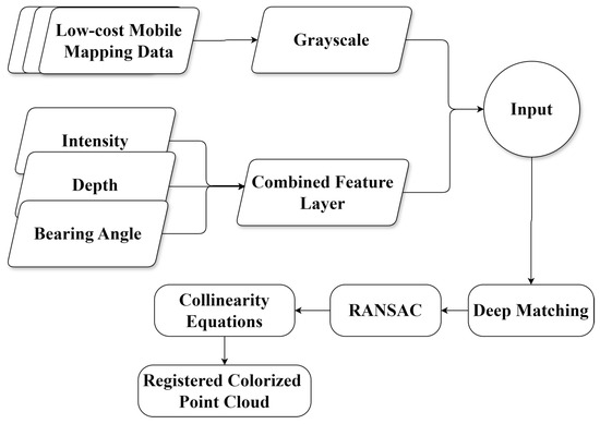
Figure 2.
Proposed optical and LiDAR data integration method.
3.1. Camera Calibration
Camera calibration is essential for camera–LiDAR registration, especially when modalities operate in different coordinate systems, as it establishes the necessary geometric transformations and projections to accurately integrate data across varying projection models, aligning the camera’s image coordinate system with LiDAR’s object coordinate system. Camera intrinsic and extrinsic parameters are estimated using 3D ground control points, often using a calibration target and their corresponding 2D image points [26,27]. For high-quality cameras, techniques like the Haris corner operator detect the checkerboard points and the Levenberg–Marquardt Optimizer [28] solves the parameters. A more advanced calibration process is necessary for the lower-cost and lower-quality cameras. This calibration involves a stepwise construction of the lens distortion model, focusing on correcting image distortions [29].
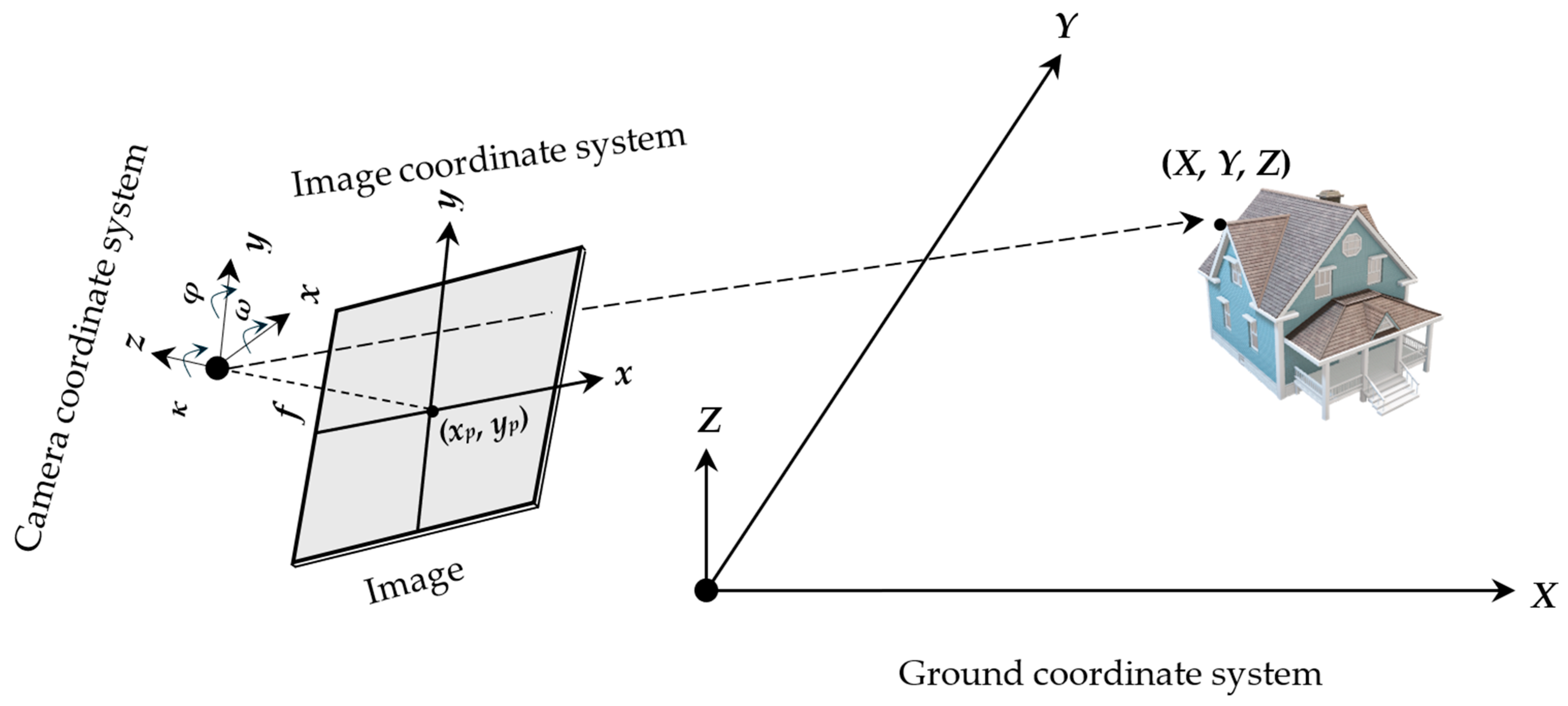
The intrinsic parameters from the calibration process specify the internal characteristics of the camera. The principal point (xp, yp) denotes the image point where the optical axis intersects the image plane, while the focal length (f) defines the scale of the projection. These parameters facilitate the central projection from 2D image to 3D camera coordinates, as depicted in Figure 3. If the intrinsic parameters are stable, the matrix of intrinsic parameters remains constant regardless of the scene observed. Once determined, the camera can move about and capture images from various scenes, provided that the focal length remains unchanged, and automatic focus is disabled. However, if an image is rescaled for sampling purposes, the focal length and principal point must be uniformly scaled by the same factor.

Figure 3.
Camera-to-ground coordinate system transformations. The rotational extrinsic parameters of the LiDAR sensor are represented by the angles (ω, φ, κ), which describe the orientation of the camera in the 3D space. The camera’s principal point is denoted by (xp, yp), and f represents the focal length. The ground coordinates are represented by (X, Y, Z), corresponding to the real-world position in the ground reference system.
Additional intrinsics include distortion coefficients such as radial (k₁, k₂, k₃) due to nonlinear magnification, causing straight lines to appear curved in the image, and decentering (p₁, p₂) due to misalignment of lens elements. Figure 3 assumes an ideal pinhole camera without a lens, neglecting lens distortion. Therefore, all images require separate undistortion before further processing, correcting geometric inaccuracies. The pixel coordinate corrections (δx, δy) are computed from the distorted pixel coordinates (x, y) using Equations (1)–(5) [30].
First, the image points are located with respect to the principal point as expressed in Equation (1). Then, the radial distance of each normalized image point is calculated as described in Equation (2):
Next, the displacement due to radial distortion (Δr) and decentering distortion (Δxdec, Δydec) are computed as shown in Equations (3) and (4), respectively. Subsequently, the x (δx) and y (δy) components are solved. These corrections adjust the x and y coordinates of the image points based on a triangle similarity relationship as expressed in Equation (5):
3.2. LiDAR Feature Layer Generation
LiDAR point cloud data are commonly collected in spherical coordinates, representing the horizontal scan angle (α), vertical scan angle (ω), and range distance (r) from the sensor’s origin to each point. In addition to this, each scanned point includes an intensity value reflected from the surface. By assuming the sensor’s local origin is at (0,0,0) and utilizing its spherical coordinates, the cartesian coordinates (X, Y, Z) can be solved through Equation (6):
The LiDAR feature layer generation process involves populating image arrays with intensity, depth, and bearing angle values. The two latter are derived from range and scan angle information. The bearing angle (BA) refers to the angle formed between the line segment joining two successive points in a laser scan and the laser beam; this can be derived using Equation (7) below [5,9,15].
where
- = current depth value in the depth image,
- = preceding depth value in the depth image, and
- Φ = laser beam scan angular step in the direction of interest.
The image size and shape are dependent on the sensors’ data characteristics. Spinning LiDAR, often used in MMS, produces an unordered set of points based on its scan lines, with the image dimensions determined by the desired geometric field of view (FOV). Conversely, fixed terrestrial LiDAR utilizes structured indexing, with the image dimensions defined by maximum rows and columns. Often, however, collected 3D point clouds are irregularly spaced. Thus, when they are mapped onto a grid, they may not align with the intended perspective or orientation or could have objects overlapping. To address this issue, rotation of the point cloud around its axes may be required to orient it correctly for the desired appearance in the image. Next, void pixels caused by occlusions and sparse data in the resulting 2D perspective are filled by adjusting the kernel size and averaging neighboring pixel values until the image matrix is complete.
The LiDAR feature layers are cropped and resized to match the spatial resolution of their corresponding optical images, aligning their pixel dimensions (rows and columns) as the matching algorithms require. This process ensures control over the aspect ratio. Subsequently, the individual feature layers are weighted and combined following the method used by Leahy and Jabari [9]. Each layer is normalized so that its pixel values fall within the range of 0 to 1. These normalized layers are then merged, with different weight combinations ensuring that the total contribution of all layers sums up to 1.
3.3. Feature Matching and Correspondence
SuperGlue and LoFTR deep learning-based offered advancements in image matching areas [23,24]. Both algorithms are trained on the MegaDepth Dataset [31], which includes indoor and outdoor scenarios.
The architecture of the graph neural network comprises two key heads: a front-end keypoint detector, called SuperPoint, and a middle-end keypoint matcher, called SuperGlue [22,23]. The raw optical image and its corresponding LiDAR feature layer undergo preprocessing using a shared encoder and parallel interest and descriptor decoders in the front end. The shared encoder preprocesses the images, reducing them to 1/8th of their original size while retaining essential channel information. Meanwhile, the interest and descriptor decoders evaluate every pixel of the images, predicting their likelihood of being a critical point and computing associated descriptors. The optimal matching layer determines the best match between key points based on their descriptors by assigning a score to each potential match. The objective is to maximize the total score of all matches, ensuring accurate and reliable feature matching across the camera and spherical LiDAR features [23].
LoFTR differs from SuperGlue as it first extracts features at a coarse level and then refines good matches at a finer level, allowing for the recognition of small details and larger structures. Utilizing transformers with self- and cross-attention mechanisms, LoFTR can focus on prevalent descriptors. Positional encoding aids in understanding the spatial layout of features within the images, particularly in scenes with sparse features. In terms of matching, LoFTR employs the same optimal transport layer as SuperGlue, assigning confidence scores to matches based on feature similarity. Despite its benefits, LoFTR has constraints, such as requiring input dimensions to be multiples of 8 and relying on GPU for computation [24].
3.4. Transformation and Registration
Registering camera–LiDAR data in different coordinate systems involves two mappings, as shown in Figure 3. First, the camera’s relative pose to the LiDAR sensor is determined using the six degrees of freedom (6DoF) camera extrinsic parameters, including rotational parameters (ω, φ, κ) and translational parameters (Xc, Yc, Zc), solved through space resection. Second, the intrinsic camera parameters, obtained through calibration, are used to project pixel coordinates into image coordinates. These two mappings happen simultaneously using the collinearity transformations [30] from Equation (8).
Space resection is used to determine the 6DoF by establishing a camera’s position and orientation (pose) based on known 3D ground control points within a scene. When 3D control points are unavailable, the 2D coordinates obtained from image-matching algorithms can be used to compute corresponding ground coordinates. This is accomplished by generating a LiDAR feature layer and embedding the geometric X, Y, and Z values within its matrices. This methodology allows for the extraction of real-world coordinates from any pixel coordinate within the image.
The 6DoF are solved iteratively for both x and y directions using Equation (8) and RANSAC to remove outliers and minimize residuals. Removing distortion from the images before matching eliminates the requirement of self-calibration in equations.
Here,
- x, y = spherical LiDAR feature coordinates,
- f = calibrated focal length,
- xp, yp = location of the principal point,
- X, Y, Z = LiDAR’s ground coordinates,
- Xc, Yc, Zc = camera location/translation, and
- mᵢⱼ = elements of rotation matrix from ground to image coordinate system.
Of note, the convention of using uppercase letters for ground coordinates and lowercase letters for image coordinates follows the mathematical notation presented by Wolf et al. [29]. Once the collinearity equation is established, the full LiDAR point cloud can be transformed into image coordinates and assigned an RGB value. This results in a registered and colorized point cloud.
4. Results
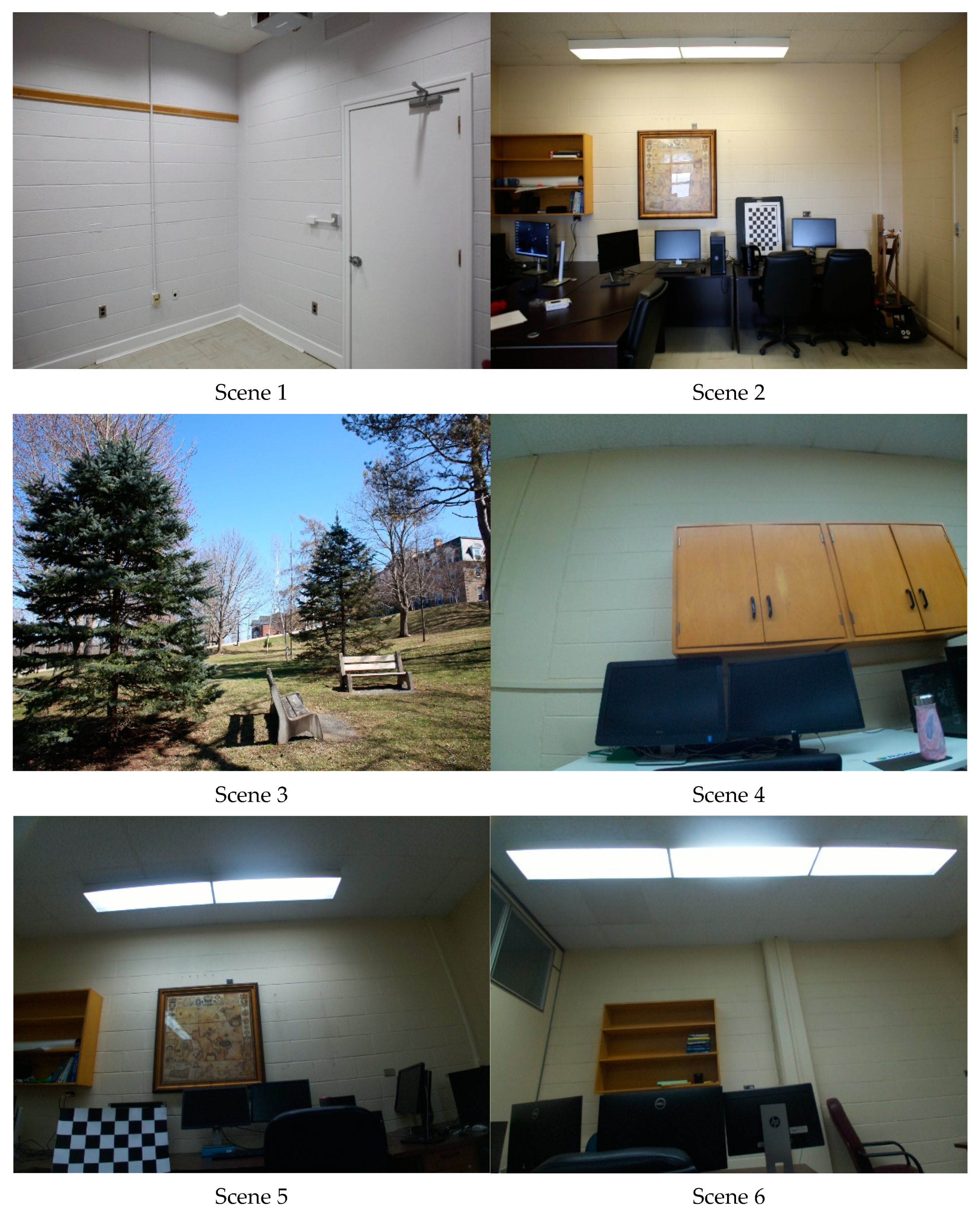
In this section, we apply our methodology to actual data collected from various sensors and scenes, as shown in Figure 4 and described in detail in Table 1. The methods were executed on a Dell all-in-one computer equipped with an Intel® Core™ i5-4570S processor, a 64-bit operating system, CPU capabilities of 2.90 GHz, and 8.00 GB of RAM. The computer was manufactured by Dell Inc., Round Rock, TX, USA. For LoFTR’s image matching transformer, additional GPU support was provided using Google Colab’s basic subscription, which grants access to Nvidia T4 GPUs. Each scene will be referred to by its respective scene number in further discussion.
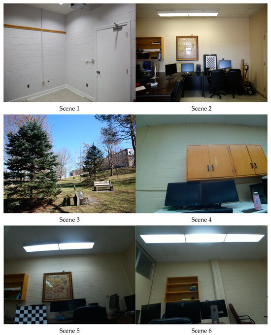
Figure 4.
The experimental scenes employed in this study. The six scenes were acquired in outdoor and indoor environments, representing different object arrangements, lighting conditions, and spatial compositions.

Table 1.
Experimental setup details.
As outlined in Table 1, the terrestrial data were collected using the survey-grade TX5 3D laser scanner (manufactured by Trimble Inc., Westminster, CO, USA) and the EOS-1D X Mark III DSLR camera (manufactured by Canon Inc., Tokyo, Japan). The LiDAR sensor uses an integrated dual-axis compensator to automatically level the captured scan data and an integrated compass and altimeter to provide orientation and height information.
The MMS data were collected using SLAMM-BOT, a custom-built platform. This platform incorporates a Arducam IMX477 Mini camera (manufactured by Arducam Technology Co., Ltd., Shenzhen, China), controlled and storing data in real-time using a Raspberry Pi board (manufactured by Raspberry Pi Foundation, Cambridge, UK) and a laptop to manage data captured by the VLP-16 LiDAR sensor (manufactured by Velodyne Lidar, Inc., San Jose, CA, USA).
4.1. Pre-Processing
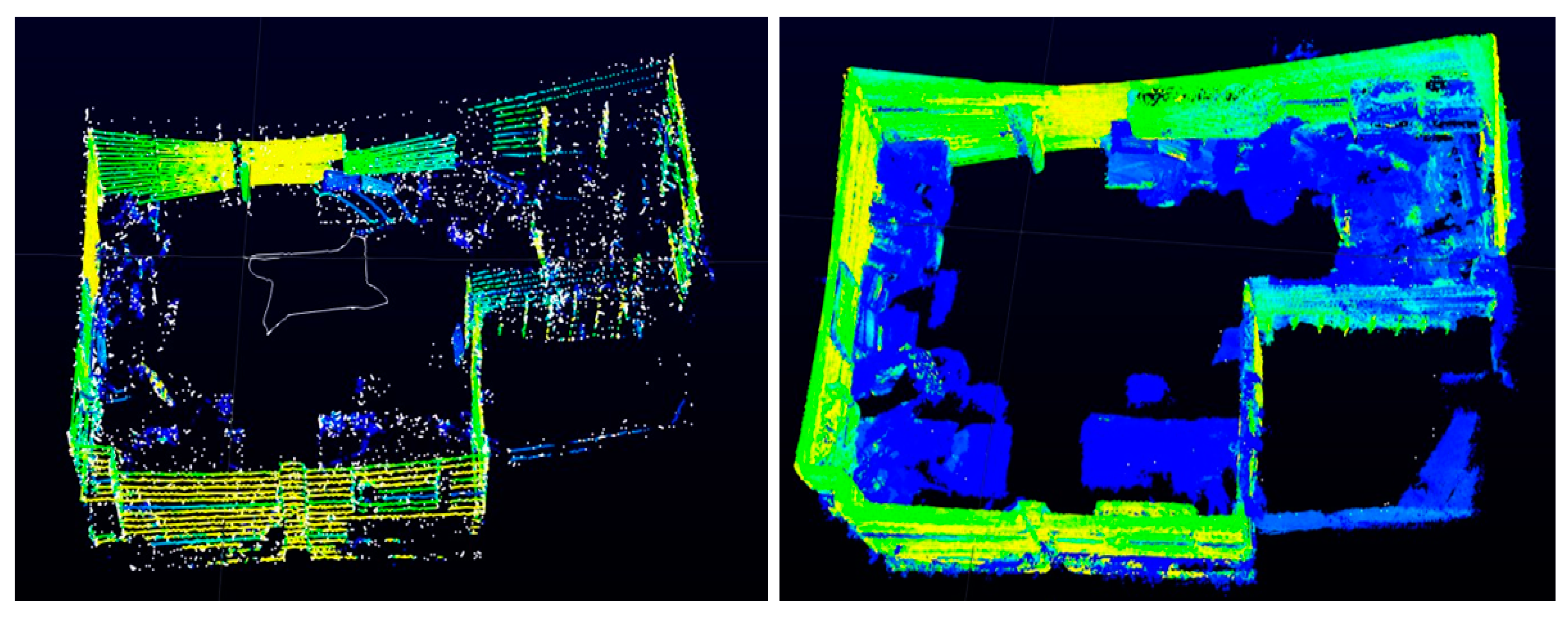
The LiDAR frames collected from SLAMM-BOT create significant gaps in the data, especially when the platform is stationary. This issue arises because the VLP-16 [32] has only 16 laser channels in its vertical FOV, resulting in considerable blank spaces between the scan lines. Consequently, when the platform is not moving, these gaps remain unfilled, leading to incomplete data coverage. To mitigate this, SLAMM-BOT is driven in a closed loop through Scenes 4 to 5 and performs SLAM [33]. SLAM identifies consistent features across sequential frames, constructing a trajectory. Subsequently, trailing frames are aggregated using a temporal transform applier [11], enhancing visual coherence and densifying the point cloud, as seen in Figure 5. This final point cloud is segmented into regions of interest (RoI) based on its corresponding optical image.
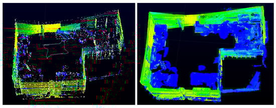
Figure 5.
Comparison of single frame (left) vs. densified aggregated frames (right).
The TX5 data are already dense and high-quality but still require FOV rotation, scaling, and cropping, as detailed in Section 3.2. The original size of the optical images in Scenes 1–3 was scaled by 0.25 to achieve a more reasonable spatial resolution to use with the matching algorithms. Given the differing sizes of the original LiDAR feature layers, each was appropriately scaled to get closer to this new dimension. Then, the rest was cropped off. Scenes 1 and 2 were scaled by 0.25, while Scene 3 was scaled by 0.5. This adjustment was necessary because the original high spatial resolution of the images creates challenges for feature matching and efficiency with SuperGlue and LoFTR. High-resolution images contain more features, increasing computational load and memory usage, and can even lead to poor matches, especially in areas with repetitive patterns.
The cameras were both pre-calibrated, as detailed in Section 3.1, to solve for the intrinsics and correct lens distortion. For the SLAMM-BOT data, k₂ and k₃ are highly correlated, allowing k₃ to be disregarded and set to 0. Moreover, the decentering coefficients were found to be insignificant and removed from the equation.
4.2. Correspondences and Registration
The processed LiDAR datasets are used to create feature layers, including intensity, depth, and bearing angle. These layers are normalized and weighted to form combined feature layers, following the methodology outlined in Section 3.2. Subsequently, the various feature layers are matched with optical images using SuperGlue and LOFTR to yield strong correspondences for registration.
For SLAMM-BOT’s data, due to the lower quality, only intensity layers were utilized. A matching threshold of 0.25 was set to ensure sufficient matches. Results are summarized in Table 2.
Table 2.
SLAMM-BOT camera–LiDAR correspondence results.
For the TX5 scenes, a matching threshold of 0.5 and a keypoint threshold of 0.1 are set, and the results of the correspondence are presented in Table 3. Within the table, the highest number of correspondences detected by each matching algorithm for every layer combination is highlighted in bold text. For visualization purposes, intensity, depth, and bearing angle layers are denoted as “I”, “D”, and “BA”, respectively. SuperGlue and LoFTR are denoted as “SG” and “L”, respectively.
Table 3.
TX5 camera–LiDAR correspondence counts using combined and weighted LiDAR feature layers. The bolded values represent the highest number of correspondences detected by each matching algorithm for every layer combination.
To evaluate transformation accuracy, the top-performing layers within each category for both SuperGlue and LoFTR are randomly divided into 70% for training and 30% for testing. The training data establish the collinearity transformation equations. The testing data are used to assess the accuracy of the models by computing the root mean square Error (RMSE) between the LiDAR feature layer pixel coordinates and the transformed optical pixel coordinates.
The residuals are then compared against their respective baselines for each dataset. In terrestrial scenes, the TX5’s built-in optical camera was matched with the LiDAR data. Matching pixel locations were manually selected across RGB images and spherical LiDAR features, dividing them into 16 sections to ensure comprehensive evaluation. For SLAMM-BOT’s baseline, an established rigid-body camera–LiDAR calibration toolbox [12] was utilized to determine its baseline reprojection error. These comparative results are presented in Table 4.
Table 4.
RMSE results for best LiDAR feature layer combinations and baseline comparisons across different image matchers. The bolded values represent the lowest RMSE for each scene.
These findings indicate that all best results outperformed their baseline. The misregistration error varied from 0.7 pixels, achieved using LoFTR for Scene 1 with a layer combination of 5% BA, 70% intensity, and 25% depth, to ~5 pixels for the lower-quality SLAMM-BOT data. Despite this variance, each range of accuracy serves valuable purposes tailored to specific application requirements and costs.
5. Discussion
This section analyses the experimental results, focusing on how different LiDAR feature layers and their weightings affect feature-matching accuracy. We also evaluate the performance of various platforms and sensors. Additionally, we compare the effectiveness of the image-matching algorithms SuperGlue and LoFTR.
5.1. LiDAR Feature Layers for Matching
The performance of different LiDAR feature layers varied across scenes and platforms. Intensity layers became apparent as the best performers across all TX5 and SLAMM-BOT datasets. The success of intensity data can be linked to its similarity to grayscale values in camera images, making it more analogous and easier for matching algorithms to process.
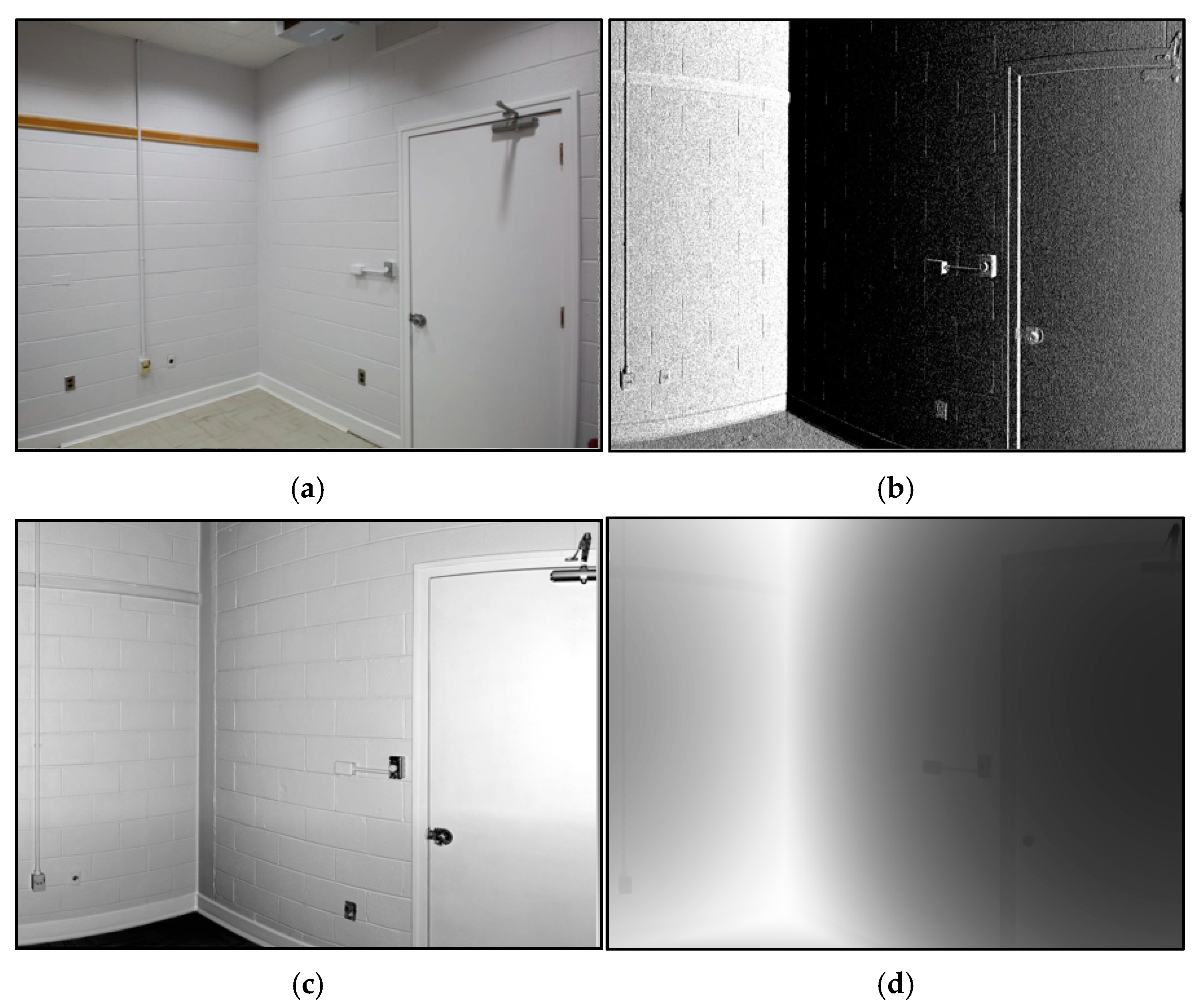
Depth layers were less effective in the TX5 and SLAMM-BOT data, except Scene 3. Based on our findings, depth images are more successful in outdoor scenes with protruding surfaces like trees, which offer more apparent visual features. Whereas scenes with limited depth variation do not provide meaningful features, like Scene 1, shown in Figure 6d. Our findings align with the current literature, where the only successful camera–LiDAR features matching with depth images, to the best of our knowledge, have been in outdoor scenes [13,18].
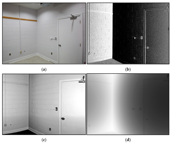
Figure 6.
Comparison of different images: (a) optical; (b) bearing angle; (c) intensity; and (d) depth.
BA layers worsened results when weighed more than 30% and did not yield notable individual layer success. Originally, it was hypothesized that poor BA performance in aerial data was due to the large range and small angle increments from the platform’s 1000-meter altitude [9], creating indistinguishable features. However, initial tests with the close-range TX5 data were more detailed, as shown in Figure 6b, where room shapes and door frames are visible. Despite this, SuperGlue and LoFTR struggled with matching the individual BA layers due to grainy and speckled variations in the image. Our findings align with previous studies. Liu et al. [15] used BA for segmentation and edge detection, not feature detection between modalities. Scaramuzza et al. [5] achieved camera–LiDAR registration with BA images only through manual matching by human observers. This indicates that automated matching with BA data needs further advancements to be effective as an individual layer or when weighted higher than 30%.
Interestingly, beyond the individual performance of single layers, combining different layers—even those like bearing angle and depth, which did not perform optimally alone—into a weighted single image did improve matching results and accuracy. By integrating layers at specific weights, subtle features like contrast and texture are captured, which might be missed by single layers alone. An example of this is shown in Table 3, where the combination of 70% intensity and 30% depth layer yields 172 correspondences for Scene 2, compared to 133 correspondences for the 100% intensity layer. Similar trends are observed across other scenes, demonstrating notably increased matches, particularly with the dual-layer approach.
Our findings reveal that in all TX5 scenes, combining layer information resulted in more feature matches, particularly Scenes 1 and 2, which gave the best registration accuracies. This underscores the advantage of a multi-layer approach in reducing registration errors.
5.2. Sensor Performance
It is beneficial to use camera and LiDAR data pairs with similar shapes and spatial resolutions. Feature matching algorithms require input images to be of identical size; so, if they are not, significant resizing or cropping of one data type may result in information loss. We found the best performance with the TX5 by scaling the original spatial resolution of optical images by 0.5 and LiDAR feature layers by 0.25 (Scenes 1 and 3) or 0.5 (Scene 2). This adjustment was necessary because higher original spatial resolutions posed matching and efficiency challenges with SuperGlue and LoFTR.
From our findings, the TX5 demonstrated the lowest RMSE, improving upon its baseline. The SLAMM-BOT, while showing a larger error due to its lower data quality and sensor capabilities, still significantly improved from its baseline. The results of the TX5 and SLAMM-BOT are not compared directly against each other due to the inherent differences in their sensor quality and data characteristics.
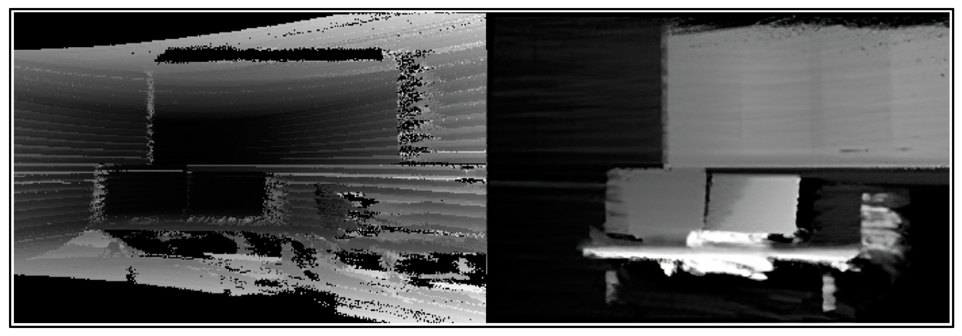
The SLAMM-BOT depth and BA layers were intentionally left out of the experiments. An investigation into its range stability revealed significant dispersions and systematic offsets between adjacent sampling lines. Chan et al. [34] suggested that the VLP-16 has an approximate 2 cm range fluctuation during the first hour of observation. Despite efforts to remedy the depth image, as illustrated in Figure 7, the VLP-16 depth image produced false matches; therefore, only the intensity data were used for evaluating SLAMM-BOT, producing viable matches shown in Figure 8.
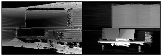
Figure 7.
Before (left) and after (right) attempts to remedy the range dispersions in the SLAMM-BOT depth image.
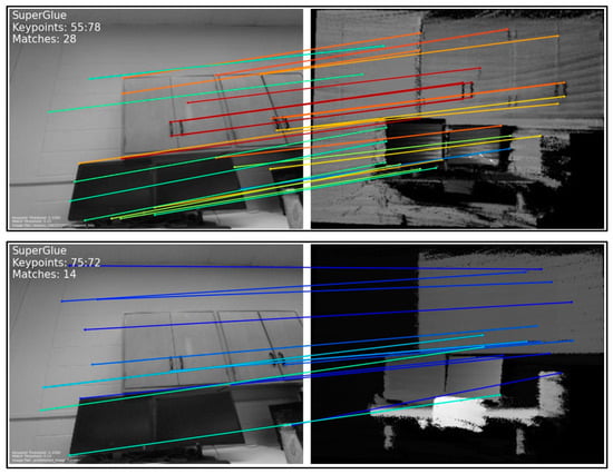
Figure 8.
Viable matches from the intensity image (top) vs. false matches from the depth image (bottom). The color scheme represents match confidence, with red representing high confidence and blue representing low confidence.
5.3. Performance of Image Matching Algorithms
SuperGlue and LoFTR performed well on all the TX5 scenes, achieving sub-pixel accuracy in the best cases. It performed reasonably well with the SLAMM-BOT scenes. This high performance can be attributed to the robust training and architecture of the algorithms, as discussed in Section 3.
We determined it was not necessary to train SuperGlue or LoFTR on LiDAR feature layers before our experiments because existing research, such as Koide et al. [6], demonstrated a strong correspondence between LiDAR intensity images and camera images in SuperGlue without pre-training. However, the potential benefits of training algorithms on LiDAR feature layers merit consideration for future research, particularly for scenes and layers with less effective performance. To our knowledge, no training dataset exists of LiDAR feature layers, particularly those that include intensity, depth, bearing angle, and weighted combinations.
6. Conclusions
In the current field, dealing with LiDAR data and camera images from different projection models without pre-registration presents a challenging registration process due to varying geometric imaging configurations. Terrestrial scene registration is particularly difficult due to occlusions, varying scales, and environmental complexity. To address these challenges and contribute to the field, this study demonstrates the importance of establishing strong camera–LiDAR correspondences for registration to advance spatial awareness across various applications in the fields of computer vision and photogrammetry.
We introduced a new registration pipeline that uses 2D spherical LiDAR features as intermediaries to align them with pre-calibrated camera images. We achieved improved cross-modal correspondences by employing deep learning feature-based image-matching algorithms like SuperGlue and LoFTR with weighted combinations of LiDAR feature layers, including intensity, depth, and bearing angle. These matches, when linked to 3D ground points and processed through collinearity equations, enabled us to register the geometry of spherical LiDAR features with the spectral information from optical images, resulting in colorized point clouds. This approach differentiates itself from existing methods by addressing challenges in aligning data sourced from distinct coordinate systems, orientations, and resolutions while achieving a higher magnitude of accurate matched features with weighted 2D feature layers.
Our findings demonstrate varying levels of accuracy influenced by sensor capabilities and cost. Achieving sub-pixel accuracy (<1–2 pixels), equivalent to approximately 3 mm median error in ground coordinates, is feasible with survey-grade LiDAR scanners and high-resolution cameras. This level of precision is crucial for demanding tasks such as establishing control networks and precision surveying [35], as well as for building extraction applications in 3D city modeling [36,37]. Conversely, our findings show that achieving lower-end accuracy (~5 pixels) with SLAMM-BOT’s spinning LiDAR and low-resolution cameras results in approximately a median error of 6 cm in ground coordinates. Despite its lower precision, this approach provides a cost-effective solution suitable for applications such as land reconnaissance, profiling, or producing digital terrain models [38].
Moving forward, future research efforts could focus on enhancing bearing angle images to achieve better spectral matching. Additionally, training the image-matching algorithms on depth layers could offer a larger amount of strong cross-modal matches to further improve registration errors. Furthermore, incorporating other LiDAR feature layers, such as zenith angle images, could serve as an additional resource to improve the matching process. The inclusion of automation in future work would be valuable, as it could replace manual preprocessing and integrate the registration steps, enabling real-time scene registration.
Author Contributions
Conceptualization, J.L. and S.J.; methodology, J.L., S.J. and D.L.; software, J.L.; validation, J.L. and S.J.; formal analysis, J.L. and S.J.; investigation, J.L., S.J. and D.L.; resources, J.L., S.J. and D.L.; data curation, J.L.; writing—original draft preparation, J.L.; writing—review and editing, J.L., S.J. and D.L.; visualization, J.L.; supervision, S.J.; project administration, S.J.; funding acquisition, S.J.; writing—review and editing, A.S. and J.L. All authors have read and agreed to the published version of the manuscript.
Funding
This research was funded by the University of New Brunswick Harrison McCain Young Scholar Research Award HMF2023 YS-13; the University of New Brunswick Faculty of Engineering distinguished lecture series; Natural Sciences and Engineering Research Council of Canada Discovery Grant RGPIN-2020-04698; and the Natural Sciences and Engineering Research Council of Canada Discovery Grant RGPIN-2018-03775.
Data Availability Statement
The data that support the findings of this study are openly available in the UNB Dataverse repository at https://doi.org/10.25545/6DGF1V. Additional data related to this study are available upon reasonable request to the corresponding author.
Acknowledgments
We acknowledge the Faculty of Engineering and the Department of Geodesy and Geomatics Engineering at the University of New Brunswick for providing a supportive research environment. We extend special thanks for the invaluable assistance and the technical support offered by the department. We also acknowledge the Government of New Brunswick for providing publicly sourced aerial ortho imagery and LiDAR data, as well as the developers of the SuperGlue [23] and LoFTR [24] image-matching pipelines.
Conflicts of Interest
The authors declare no conflicts of interest.
References
- Wang, X.Y.; Zhang, P.P.; Dou, M.S.; Tian, S.H. A Review of Image and Point Cloud Fusion in Autonomous Driving. In Proceedings of the 6GN for Future Wireless Networks, Shanghai, China, 7–8 October 2023; Li, J., Zhang, B., Ying, Y., Eds.; Springer Nature Switzerland: Cham, Switzerland, 2024; pp. 62–73. [Google Scholar]
- Yan, G.; He, F.; Shi, C.; Wei, P.; Cai, X.; Li, Y. Joint Camera Intrinsic and LiDAR-Camera Extrinsic Calibration. In Proceedings of the 2023 IEEE International Conference on Robotics and Automation (ICRA), London, UK, 29 May–2 June 2023; IEEE: Piscataway, NJ, USA, 2023; pp. 11446–11452. [Google Scholar]
- Zhou, L.; Li, Z.; Kaess, M. Automatic Extrinsic Calibration of a Camera and a 3D LiDAR Using Line and Plane Correspondences. In Proceedings of the 2018 IEEE/RSJ International Conference on Intelligent Robots and Systems (IROS), Madrid, Spain, 1–5 October 2018; pp. 5562–5569. [Google Scholar]
- Levinson, J.; Thrun, S. Automatic Online Calibration of Cameras and Lasers. In Proceedings of the Robotics: Science and Systems IX, Berlin, Germany, 24–28 June 2013; pp. 29–36. [Google Scholar]
- Scaramuzza, D.; Harati, A.; Siegwart, R. Extrinsic Self Calibration of a Camera and a 3D Laser Range Finder from Natural Scenes. In Proceedings of the 2007 IEEE/RSJ International Conference on Intelligent Robots and Systems, San Diego, CA, USA, 29 October–2 November 2007; pp. 4164–4169. [Google Scholar]
- Koide, K.; Oishi, S.; Yokozuka, M.; Banno, A. General, Single-Shot, Target-Less, and Automatic LiDAR-Camera Extrinsic Calibration Toolbox. In Proceedings of the 2023 IEEE International Conference on Robotics and Automation (ICRA), London, UK, 29 May–2 June 2023; pp. 11301–11307. [Google Scholar]
- Zhang, J.; Lin, X. Advances in Fusion of Optical Imagery and LiDAR Point Cloud Applied to Photogrammetry and Remote Sensing. Int. J. Image Data Fusion 2017, 8, 1–31. [Google Scholar] [CrossRef]
- Zhu, B.; Ye, Y.; Zhou, L.; Li, Z.; Yin, G. Robust Registration of Aerial Images and LiDAR Data Using Spatial Constraints and Gabor Structural Features. ISPRS J. Photogramm. Remote Sens. 2021, 181, 129–147. [Google Scholar] [CrossRef]
- Leahy, J.; Jabari, S. Enhancing Aerial Camera-LiDAR Registration through Combined LiDAR Feature Layers and Graph Neural Networks. Int. Arch. Photogramm. Remote Sens. Spat. Inf. Sci. 2024, 48, 25–31. [Google Scholar] [CrossRef]
- Fischler, M.A.; Bolles, R.C. Random Sample Consensus: A Paradigm for Model Fitting with Applications to Image Analysis and Automated Cartography. In Readings in Computer Vision; Elsevier: Amsterdam, The Netherlands, 1987; pp. 726–740. ISBN 978-0-08-051581-6. [Google Scholar]
- LiDARView. Available online: https://lidarview.kitware.com (accessed on 1 September 2023).
- MathWorks MATLAB. Lidar and Camera Calibration. Available online: https://www.mathworks.com/help/lidar/ug/lidar-and-camera-calibration.html (accessed on 1 October 2023).
- Li, Y.; Li, H. LiDAR-Based Initial Global Localization Using Two-Dimensional (2D) Submap Projection Image (SPI). In Proceedings of the 2021 IEEE International Conference on Robotics and Automation (ICRA), Xi’an, China, 30 May–5 June 2021; pp. 5063–5068. [Google Scholar]
- Dong, W.; Ryu, K.; Kaess, M.; Park, J. Revisiting LiDAR Registration and Reconstruction: A Range Image Perspective. arXiv 2022, arXiv:2112.02779. [Google Scholar]
- Liu, Y.; Wang, F.; Dobaie, A.M.; He, G.; Zhuang, Y. Comparison of 2D Image Models in Segmentation Performance for 3D Laser Point Clouds. Neurocomputing 2017, 251, 136–144. [Google Scholar] [CrossRef]
- Park, J.; Zhou, Q.-Y.; Koltun, V. Colored Point Cloud Registration Revisited. In Proceedings of the 2017 IEEE International Conference on Computer Vision (ICCV), Venice, Italy, 22–29 October 2017; pp. 143–152. [Google Scholar]
- Lowe, D.G. Distinctive Image Features from Scale-Invariant Keypoints. Int. J. Comput. Vis. 2004, 60, 91–110. [Google Scholar] [CrossRef]
- Abedinia, A.; Hahnb, M.; Samadzadegana, F. An Investigation into the Registration of LIDAR Intensity Data and Aerial Images Using the SIFT Approach. Int. Arch. Photogramm. Remote Sens. Spat. Inf. Sci. 2008, XXXVII, 169–176. [Google Scholar]
- Bay, H.; Ess, A.; Tuytelaars, T.; Van Gool, L. Speeded-Up Robust Features (SURF). Comput. Vis. Image Underst. 2008, 110, 346–359. [Google Scholar] [CrossRef]
- Karami, E.; Prasad, S.; Shehata, M. Image Matching Using SIFT, SURF, BRIEF and ORB: Performance Comparison for Distorted Images. Available online: https://arxiv.org/abs/1710.02726v1 (accessed on 27 September 2024).
- Zhang, X.; Zhang, A.; Meng, X. Automatic Fusion of Hyperspectral Images and Laser Scans Using Feature Points. J. Sens. 2015, 2015, 415361. [Google Scholar] [CrossRef]
- DeTone, D.; Malisiewicz, T.; Rabinovich, A. SuperPoint: Self-Supervised Interest Point Detection and Description. In Proceedings of the 2018 IEEE/CVF Conference on Computer Vision and Pattern Recognition Workshops (CVPRW), Salt Lake City, UT, USA, 18–22 June 2018; pp. 337–33712. [Google Scholar]
- Sarlin, P.-E.; DeTone, D.; Malisiewicz, T.; Rabinovich, A. SuperGlue: Learning Feature Matching With Graph Neural Networks. In Proceedings of the 2020 IEEE/CVF Conference on Computer Vision and Pattern Recognition (CVPR), Seattle, WA, USA, 13–19 June 2020; IEEE: Piscataway, NJ, USA, 2020; pp. 4937–4946. [Google Scholar]
- Sun, J.; Shen, Z.; Wang, Y.; Bao, H.; Zhou, X. LoFTR: Detector-Free Local Feature Matching with Transformers. In Proceedings of the 2021 IEEE/CVF Conference on Computer Vision and Pattern Recognition (CVPR), Nashville, TN, USA, 20–25 June 2021; IEEE: Piscataway, NJ, USA, 2021; pp. 8918–8927. [Google Scholar]
- Zhang, Y.; Zhao, X. MESA: Matching Everything by Segmenting Anything. Available online: https://arxiv.org/abs/2401.16741v2 (accessed on 27 September 2024).
- Fetic, A.; Juric, D.; Osmankovic, D. The Procedure of a Camera Calibration Using Camera Calibration Toolbox for MATLAB. In Proceedings of the 35th International Convention MIPRO, Opatija, Croatia, 21–25 May 2012. [Google Scholar]
- Heikkila, J.; Silven, O. A Four-Step Camera Calibration Procedure with Implicit Image Correction. In Proceedings of the IEEE Computer Society Conference on Computer Vision and Pattern Recognition, San Juan, PR, USA, 17–19 June 1997; IEEE: Piscataway, NJ, USA, 1997; pp. 1106–1112. [Google Scholar]
- More, J.J. Levenberg—Marquardt Algorithm: Implementation and Theory; Argonne National Laboratory: Lemont, IL, USA, 1977. [Google Scholar]
- Zhang, Z. A Flexible New Technique for Camera Calibration. IEEE Trans. Pattern Anal. Machine Intell. 2000, 22, 1330–1334. [Google Scholar] [CrossRef]
- Wolf, P.R.; Dewitt, B.A.; Wilkinson, B.E. Elements of Photogrammetry with Applications in GIS, 4th ed.; McGraw-Hill Education: New York, NY, USA, 2014; ISBN 978-0-07-176112-3. [Google Scholar]
- Li, Z.; Snavely, N. MegaDepth: Learning Single-View Depth Prediction from Internet Photos. In Proceedings of the IEEE Conference on Computer Vision and Pattern Recognition, Salt Lake City, UT, USA, 18–23 June 2018. [Google Scholar]
- Velodyne LiDAR. Available online: https://ouster.com/products/hardware/vlp-16 (accessed on 1 August 2023).
- Zhang, J.; Singh, S. LOAM: Lidar Odometry and Mapping in Real-Time. In Proceedings of the Robotics: Science and Systems X, Berkeley, CA, USA, 12–16 July 2014. [Google Scholar]
- Chan, T.; Lichti, D.D.; Roesler, G.; Cosandier, D.; Durgham, K. Range Scale-Factor Calibration of the Velodyne VLP-16 Lidar System for Position Tracking Applications. In Proceedings of the 11th International Conference on Mobile Mapping, Shenzhen, China, 6–8 May 2019; pp. 6–8. [Google Scholar]
- Abdullah, Q. The ASPRS Positional Accuracy Standards, Edition 2: The Geospatial Mapping Industry Guide to Best Practices. Photogramm. Eng. Remote Sens. 2023, 89, 581–588. [Google Scholar] [CrossRef]
- Awrangjeb, M.; Fraser, C.S. Automatic Segmentation of Raw LIDAR Data for Extraction of Building Roofs. Remote Sens. 2014, 6, 3716–3751. [Google Scholar] [CrossRef]
- Gilani, S.A.N.; Awrangjeb, M.; Lu, G. An Automatic Building Extraction and Regularisation Technique Using LiDAR Point Cloud Data and Orthoimage. Remote Sens. 2016, 8, 258. [Google Scholar] [CrossRef]
- Jiménez-Jiménez, S.I.; Ojeda-Bustamante, W.; Marcial-Pablo, M.; Enciso, J. Digital Terrain Models Generated with Low-Cost UAV Photogrammetry: Methodology and Accuracy. ISPRS Int. J. Geo-Inf. 2021, 10, 285. [Google Scholar] [CrossRef]


Disclaimer/Publisher’s Note: The statements, opinions and data contained in all publications are solely those of the individual author(s) and contributor(s) and not of MDPI and/or the editor(s). MDPI and/or the editor(s) disclaim responsibility for any injury to people or property resulting from any ideas, methods, instructions or products referred to in the content. |
© 2025 by the authors. Licensee MDPI, Basel, Switzerland. This article is an open access article distributed under the terms and conditions of the Creative Commons Attribution (CC BY) license (https://creativecommons.org/licenses/by/4.0/).