Estimating Winter Wheat Canopy Chlorophyll Content Through the Integration of Unmanned Aerial Vehicle Spectral and Textural Insights

Abstract

Chlorophyll content is an essential parameter for evaluating the growth condition of winter wheat, and its accurate monitoring through remote sensing is of great significance for early warnings about winter wheat growth. In order to investigate unmanned aerial vehicle (UAV) multispectral technology’s capability to estimate the chlorophyll content of winter wheat, this study proposes a method for estimating the relative canopy chlorophyll content (RCCC) of winter wheat based on UAV multispectral images. Concretely, an M350RTK UAV with an MS600 Pro multispectral camera was utilized to collect data, immediately followed by ground chlorophyll measurements with a Dualex handheld instrument. Then, the band information and texture features were extracted by image preprocessing to calculate the vegetation indices (VIs) and the texture indices (TIs). Univariate and multivariate regression models were constructed using random forest (RF), backpropagation neural network (BPNN), kernel extremum learning machine (KELM), and convolutional neural network (CNN), respectively. Finally, the optimal model was utilized for spatial mapping. The results provided the following indications: (1) Red-edge vegetation indices (RIs) and TIs were key to estimating RCCC. Univariate regression models were tolerable during the flowering and filling stages, while the superior multivariate models, incorporating multiple features, revealed more complex relationships, improving R² by 0.35% to 69.55% over the optimal univariate models. (2) The RF model showed notable performance in both univariate and multivariate regressions, with the RF model incorporating RIS and TIS during the flowering stage achieving the best results (R²_train = 0.93, RMSE_train = 1.36, RPD_train = 3.74, R²_test = 0.79, RMSE_test = 3.01, RPD_test = 2.20). With more variables, BPNN, KELM, and CNN models effectively leveraged neural network advantages, improving training performance. (3) Compared to using single-feature indices for RCCC estimation, the combination of vegetation indices and texture indices increased from 0.16% to 40.70% in the R² values of some models. Integrating UAV multispectral spectral and texture data allows effective RCCC estimation for winter wheat, aiding wheatland management, though further work is needed to extend the applicability of the developed estimation models.

1. Introduction

As a vital food crop worldwide, the growth condition of winter wheat is directly related to food security [1]. Chlorophyll content is one of the most critical indicators of physiological status for winter wheat, which significantly impacts the photosynthetic efficiency of crops, health, and yield prediction [2]. Even with this, traditional methods of measuring chlorophyll content usually rely on destructive sampling and laboratory analysis, which are time-consuming, laborious, and challenging to apply efficiently on a large scale [3]. Currently, there is a close correlation between data obtained from handheld Dualex chlorophyll meters and chlorophyll content chemically analyzed in a laboratory setting [4]. Although The Dualex collection method offers more convenience than traditional chlorophyll measurement techniques and allows for non-destructive sampling [5,6], its point-of-measurement limitations impose a certain amount of labor cost, resulting in small-scale operations and inefficiencies, which make it challenging to meet the demand for large-scale collection of crop chlorophyll content information [7,8].

In recent years, UAV-based multispectral monitoring has emerged as a highly effective tool for rapidly assessing crops’ physicochemical properties. Characterized by its operational flexibility, high spatial resolution, and extensive coverage [9], this approach has demonstrated significant potential in studies focusing on various crop parameters, including leaf area [10], above-ground biomass [11], and nitrogen content [12]. Notably, UAV multispectral imaging has been successfully applied to estimate the chlorophyll content in winter wheat. For instance, Zhang et al. [13] utilized UAV-acquired multispectral data to identify critical spectral bands and vegetation indices for assessing chlorophyll content at both the leaf and canopy levels, achieving reliable predictions. Similarly, Wang et al. [14] integrated prioritized vegetation indices with the most correlated features into a support vector machine model, demonstrating its robust capability to estimate winter wheat chlorophyll content across different moisture conditions and growth stages. Analysis of previous studies reveals that significant progress has been made in estimating chlorophyll content using spectral information, such as characteristic bands and vegetation indices, as input variables. Nonetheless, relying solely on spectral information often fails to capture the full complexity of crop growth and canopy structure, particularly under heterogeneous farmland conditions [15,16]. For instance, factors such as uneven crop densities, variable lighting conditions, and intricate soil backgrounds can interfere with spectral signals, complicating the accurate estimation of chlorophyll content [17]. Moreover, vegetation indices tend to reach saturation under high chlorophyll levels, further limiting the precision of estimation models [18]. Integrating additional data sources is crucial to overcoming these challenges and enhancing the performance, accuracy, and robustness of chlorophyll inversion models. Texture information, with its unique ability to capture the geometric structure and spatial distribution of crop features, presents a promising avenue for improving the estimation of crops’ physicochemical parameters [19].

To further improve the accuracy of chlorophyll content inversion, especially the adaptability under complex environmental conditions, scholars have applied texture information to their research and have gained practical experience. The application of texture information mainly includes texture features and texture indices [20]. For illustration, Li et al. [21] extracted eight texture features of images using the gray-level covariance matrix (GLCM) and combined them with spectral indices to improve the accuracy of estimations of the chlorophyll content of maize canopies. Wang et al. [22] explored the use of multispectral VIs combined with TIs to estimate the relative chlorophyll content in rice leaves, and the resulting combination of spectral and texture data could improve the accuracy of rice SPAD estimation at all growth stages compared with spectral data alone.

Concurrently, numerous machine learning algorithms have been widely applied to monitor chlorophyll content in winter wheat with the continuous advancement of artificial intelligence technology [23,24]. However, the type of information in the input variables and the number of input variables may significantly affect the algorithm’s performance [25,26,27]. Thus, selecting the appropriate combination of spectral information and input variables is crucial for predicting the chlorophyll content of winter wheat. So far, limited research has explored the integration of TIs with VIs for estimating winter wheat chlorophyll content, and few studies have explored the adaptability of machine learning algorithms with single and multiple input variables.

To integrate the above research status, this study was based on the UAV multispectral data of the winter wheat canopy, selecting relevant VIs based on spectral information, constructing TIs based on image texture features, and exploring the effectiveness of four models (RF, KELM, BP, and CNN) in estimating RCCC in winter wheat by using univariate and multivariate regression. The research objectives of this study were to (1) explore the advantages of combining multiple vegetation indices in estimating the chlorophyll content of winter wheat and to make up for the instability of a single vegetation index; (2) construct regression models combining vegetation indices and texture indices and compare them with models for the single type of index to assess its effect on the predictive performance of the model; and (3) evaluate the performance of different machine learning algorithms (RF, KELM, BP, CNN) in univariate and multivariate regressions to optimize the model for chlorophyll content prediction.

2. Materials and Methods

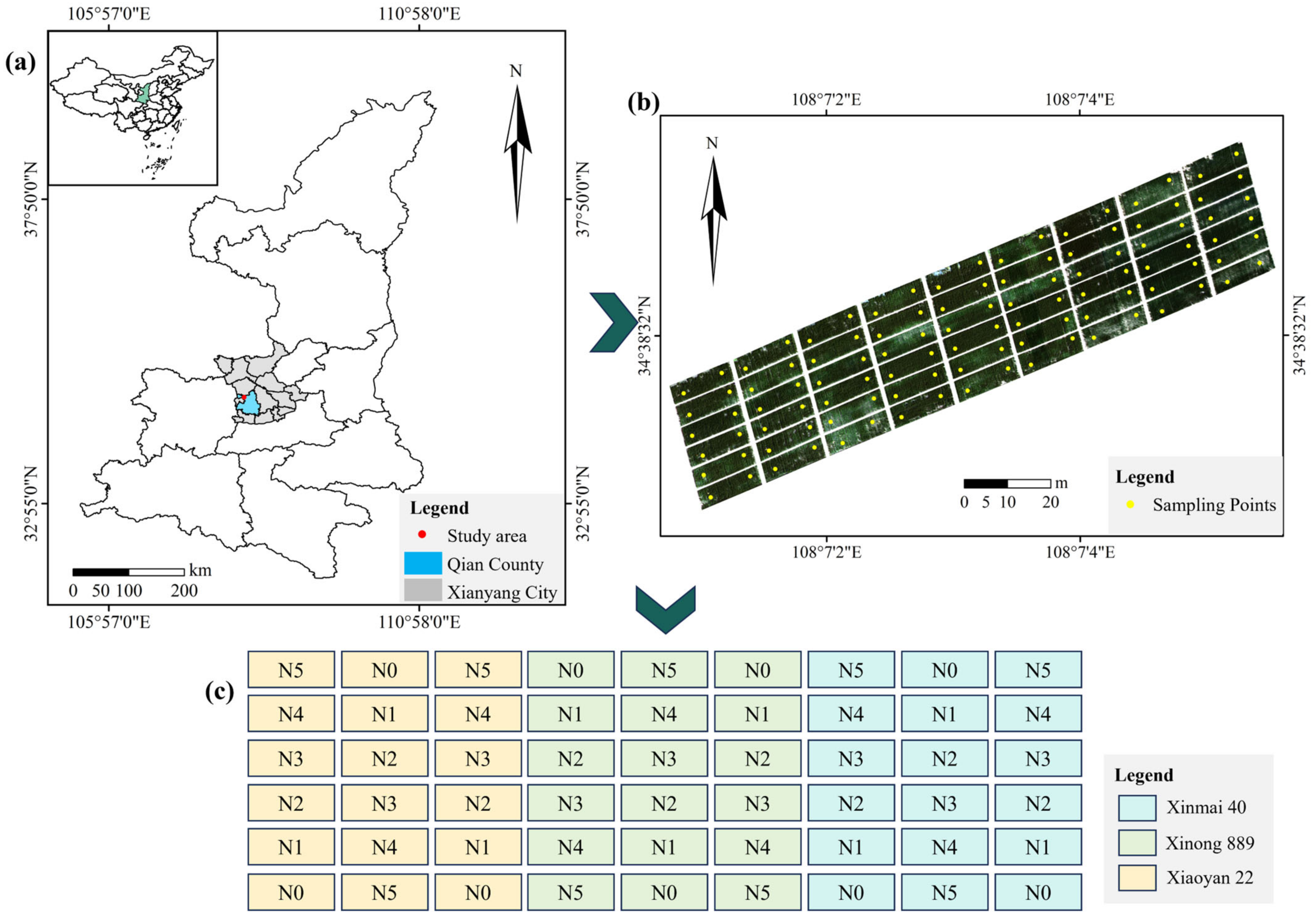
2.1. Location of the Study Area and Experimental Design

This study was conducted in Qinan Village, Liangshan Town, Xianyang, Shaanxi Province, with the location and experimental design detailed in Figure 1 and

Table 1. The time information of the experiment.

Year	Variety	Date	Growth Stage Description
2023–2024	Xiaoyan22, Xinong889, and Xinmai40	28 April	Heading Stage
		15 May	Flowering Stage
		24 May	Filling Stage

. The research focused on three winter wheat varieties—Xiaoyan22, Xinong889, and Xinmai40—during the 2023–2024 growing season. The study area, situated at an elevation of 830 m, experiences an annual average temperature of 12.6 °C and receives approximately 539 mm of rainfall. The soil is classified as red loam. Winter wheat was sown on 30 September 2023 and harvested on 11 June 2024.

The experimental design included 54 plots, each measuring 4 m × 15 m, with treatments involving six nitrogen application rates (0, 60, 90, 120, 160, and 240 kg/ha) combined with phosphorus (90 kg/ha) and potassium (60 kg/ha) fertilizers applied at sowing. No additional fertilization was performed after planting. Standard local agricultural management practices were followed throughout the entire growing season. The design aims to systematically assess the effects of nitrogen fertilizer while ensuring that phosphorus and potassium do not influence the results, aligning the fertilization treatments with actual agricultural needs. The plot size and number are appropriate to ensure the experiment’s repeatability and stability. Additionally, the cultivation of three different winter wheat varieties introduces variations in growth, providing an opportunity to explore the generalizability of the findings and simulate multi-variety cultivation scenarios. Compared to the experimental designs of Wang et al. [24] and Chen et al. [28], this design has the advantage of better control of variables, enabling precise evaluation of nitrogen fertilizer’s effects. It also ensures uniform distribution of treatments and accounts for growth differences, thereby enhancing the applicability of the results in practical agricultural management.

To ensure systematic data collection, two sampling points were established diagonally at uniform growth areas within each plot, resulting in a total of 108 sampling locations. Field data were collected at three key phenological stages: heading (28 April 2024), flowering (15 May 2024), and filling (24 May 2024), providing a robust dataset for subsequent analysis and experiments.

2.2. Data Acquisition

2.2.1. UAV Image Data Collection and Preprocessing

Under clear weather conditions, between 11:00 and 13:00, images were collected using the MS600 Pro multispectral camera (Yusense, Changchun, China) mounted on the DJI M350RTK drone platform (Da-Jiang Innovations, Shenzhen, China). This camera is equipped with six spectral bands: a blue band (centered at 450 nm, bandwidth 30 nm), a green band (centered at 555 nm, bandwidth 27 nm), a red band (centered at 660 nm, bandwidth 22 nm), two red-edge bands (centered at 720 nm and 750 nm, both with bandwidths of 10 nm), and an NIR band (centered at 840 nm, bandwidth 30 nm).

The drone was controlled using the DJI GS Pro station to fly at an altitude of 30 m, using an equidistant photo capture mode with side and forward overlap rates of 70% and 80%, respectively. The ground resolution of the MS600 Pro multispectral camera at this altitude is 2.163 m. Radiometric calibration of the multispectral images was performed using a gray board with a reflectance of 60%, which was positioned 1.2 m vertically from the camera during the initial takeoff and just before landing.

For image processing, Yusense Map software (version 2.2.5; Yusense, Changchun, China) was utilized for image stitching, orthorectification, geocorrection, and radiometric correction. Subsequently, shapefile data for 108 sample points were manually collected, and VIs for each point were calculated using R software (version 4.1.3; R Core Team, Vienna, Austria, 2021).

2.2.2. Collecting Relative Canopy Chlorophyll Content

The RCCC was quantified using the Dualex 4 (FORCE-A, Orsay, France), which employs two near-infrared light beams at 710 and 850 nm to irradiate the leaves. The 710 nm beam measures chlorophyll content within the leaves, while the 850 nm beam assesses the interference caused by the leaf structure on the chlorophyll measurement. By analyzing the transmittance of these two beams, the chlorophyll absorption rate of the leaves is calculated, with results expressed in µg/cm². Studies have demonstrated a high linear correlation between the measurements from the Dualex polyphenol–chlorophyll meter and the total chlorophyll content, with a correlation coefficient close to 1, indicating that the measurements accurately reflect the chlorophyll content of the plants [7,29].

Following the collection of UAV image data, ground measurements of chlorophyll in the wheat canopy were conducted using the Dualex 4. Ten leaves were selected from the canopy, with each leaf measured 15 times—5 times at the tip, midsection, and base, respectively—to calculate an average value, thereby obtaining a representative RCCC.

2.3. Image Feature Extraction

2.3.1. Vegetation Index Extraction

VIs are mathematical calculations of the reflectance from two or more spectral bands, serving as essential representations of multispectral information, which characterizes the spectral features of the crop canopy. For promising modeling accuracy, fifteen VIs demonstrating a strong correlation with the RCCC were selected. These indices were derived from six spectral bands of the multispectral camera, including eight RIs. The formulas for the selected VIs are detailed in

Table 2. Vegetation indices.

Definition	Calculation Formula	References
Normalized pigment chlorophyll ratio index (NPCI)	$(\mathrm{R}-\mathrm{B})/(\mathrm{R}+\mathrm{B})$	[30]
Visible-band difference vegetation index (VDVI)	$(2\mathrm{G}-\left(\mathrm{R}+\mathrm{B}\right))/(2\mathrm{G}+\left(\mathrm{R}+\mathrm{B}\right))$	[31]
Normalized difference vegetation index (NDVI)	$(\mathrm{N}\mathrm{I}\mathrm{R}-\mathrm{R})/(\mathrm{N}\mathrm{I}\mathrm{R}+\mathrm{R})$	[32]
Green normalized difference vegetation index (GNDVI)	$(\mathrm{N}\mathrm{I}\mathrm{R}-\mathrm{G})/(\mathrm{N}\mathrm{I}\mathrm{R}+\mathrm{G})$	[32]
Green chlorophyll index (GCI)	$\mathrm{N}\mathrm{I}\mathrm{R}/\mathrm{G}-1$	[33]
Simple ratio (SR)	$\mathrm{N}\mathrm{I}\mathrm{R}/\mathrm{R}$	[34]
Modified simple ratio (MSR)	$(\mathrm{N}\mathrm{I}\mathrm{R}/\mathrm{R}-1)/(\mathrm{N}\mathrm{I}\mathrm{R}/\mathrm{R}+1)$	[35]
Red-edge simple ratio (RESR720)	$\mathrm{R}/{\mathrm{R}\mathrm{E}}_{720}$	[36]
Red-edge simple ratio (RESR750)	$\mathrm{R}/{\mathrm{R}\mathrm{E}}_{750}$	[36]
Leaf chlorophyll index (LCI720)	$(\mathrm{N}\mathrm{I}\mathrm{R}-{\mathrm{R}\mathrm{E}}_{720})/(\mathrm{N}\mathrm{I}\mathrm{R}+\mathrm{R})$	[30]
Leaf chlorophyll index (LCI750)	$(\mathrm{N}\mathrm{I}\mathrm{R}-{\mathrm{R}\mathrm{E}}_{750})/(\mathrm{N}\mathrm{I}\mathrm{R}+\mathrm{R})$	[30]
Normalized difference red-edge (NDRE720)	$(\mathrm{N}\mathrm{I}\mathrm{R}-{\mathrm{R}\mathrm{E}}_{720})/(\mathrm{N}\mathrm{I}\mathrm{R}+{\mathrm{R}\mathrm{E}}_{720})$	[37]
Normalized difference red-edge (NDRE750)	$(\mathrm{N}\mathrm{I}\mathrm{R}-{\mathrm{R}\mathrm{E}}_{750})/(\mathrm{N}\mathrm{I}\mathrm{R}+{\mathrm{R}\mathrm{E}}_{750})$	[37]
Red-edge chlorophyll index (RECI720)	$\mathrm{N}\mathrm{I}\mathrm{R}/{\mathrm{R}\mathrm{E}}_{720}-1$	[38]
Red-edge chlorophyll index (RECI750)	$\mathrm{N}\mathrm{I}\mathrm{R}/{\mathrm{R}\mathrm{E}}_{750}-1$	[38]

Note: B, G, R, RE₇₂₀, RE₇₅₀, and NIR represent the blue band (centered at 450 nm), green band (centered at 555 nm), red band (centered at 660 nm), red-edge band (centered at 720 nm), red-edge band (centered at 750 nm), and near-infrared band (centered at 840 nm), respectively. The RESR₇₂₀ and RESR₇₅₀, which represent the red-edge simple ratio indices composed of the red-edge bands with central wavelengths of 720 nm and 750 nm, respectively, follow the same principle as LCI, NDRE, and RECI.

.

2.3.2. Texture Feature Extraction

This study conducted texture analysis using the GLCM [39]. Considering the sowing hole spacing of about 0.1 m, planting 10 to 20 seeds per hole, and given the image precision of the multispectral camera at about 0.021 cm/pixel, a 3 × 3 window size was selected for texture extraction. After radiometric calibration, texture features for each band were computed using ENVI software (version 5.3; Harris Geospatial Solutions, Broomfield, CO, USA), including mean, variance, homogeneity, contrast, dissimilarity, entropy, second moment, and correlation, totaling 48 texture features. The study also used PyCharm software (version 2024.1; JetBrains, Prague, Czech Republic) to calculate texture indices, including DTI, RTI, and NDTI. The definitions of texture indices are given in

Table 3. Texture indices.

Definition	Calculation Formula	References
Difference texture index (DTI)	$\mathrm{t}1-\mathrm{t}2$	[40]
Ratio texture index (RTI)	$\mathrm{t}1/\mathrm{t}2$	[40]
Normalized difference texture index (NDTI)	$(\mathrm{t}1-\mathrm{t}2)/(\mathrm{t}1+\mathrm{t}2)$	[40]

Note: t1 and t2 represent the texture feature values of arbitrary bands.

.

2.4. Modeling Approaches

In this study, the regression algorithms were implemented in the Matlab 2023b (Matrix Laboratory, MathWorks, Natick, MA, USA).

The RF is an integrated learning method for classification or regression problems that involves constructing multiple decision trees [41]. Each decision tree is trained based on a random subset of the original data, which introduces randomness and reduces the risk of overfitting the model to specific data. Subsequently, RF utilizes the predictions from multiple decision trees to improve the overall model accuracy and robustness by voting or averaging [42]. In this study, the hyperparameters of the RF model include the number of trees (n_estimators), the maximum depth of the trees (max_depth), and the minimum number of samples required for leaf nodes (min_samples_leaf), with candidate values set as follows: n_estimators = [50, 100, 500], max_depth = [None, 5, 10], and min_samples_split = [2, 3, 4].

The BPNN, initially introduced in 1986 by a team of scientists led by Rumelhart and McClelland, is a multilayer feed-forward network trained using the error backpropagation algorithm [43]. BPNN has become one of the most widely adopted neural network models due to its unique architecture and efficient training methodology. Its primary strength lies in its powerful learning and storage capabilities, which allow it to manage complex input–output mapping relationships. Importantly, BPNN does not require prior knowledge of the intricate mathematical relationships governing these mappings; instead, it learns them directly through training [44]. The learning process in BPNN employs the gradient descent method, where the network continuously adjusts its weights and biases via backpropagation to minimize the sum of squared errors. The typical architecture of a BPNN consists of an input layer, one or more hidden layers, and an output layer [45]. In this study, the hyperparameters of the BPNN model include the number of hidden layers (hidden_layer_sizes), the initial learning rate (learning_rate_init), and the maximum number of iterations (max_iter), with candidate values as follows: hidden_layer_sizes = [6, 9, 20], learning_rate_init = [0.001, 0.01], and max_iter = [500, 1000].

The KELM is a single hidden-layer feed-forward neural network that utilizes kernel functions, making it particularly well suited for handling nonlinear regression problems [46]. One of the essential advantages of KELM lies in its rapid learning ability, which makes it highly efficient when dealing with large-scale datasets [47]. However, its computational complexity is primarily influenced by the number of training samples, which can limit its performance in time-sensitive applications [48]. In this study, the hyperparameters of the KELM model include the kernel type (kernel), the regularization parameter (C), and the kernel function parameter (gamma), with candidate values specified as follows: kernel = [‘linear’, ‘rbf’], C = [10, 30, 50], and gamma = [0.1, 1].

The CNN is a feed-forward neural network characterized by its deep structure and the use of convolutional operations, making it one of the fundamental algorithms in deep learning [49]. Inspired by the mechanisms of biological visual perception, CNNs can perform supervised and unsupervised learning tasks [50]. The architecture leverages convolutional kernel parameter sharing and sparse connections between layers, significantly reducing the computational cost of processing complex topological features [51]. In this study, the hyperparameters of the CNN model include the learning rate (learning_rate), batch size (batch_size), the number of epochs (epochs), the size of the convolution kernel (kernel_size), the size of the pooling layer (pool_size), and the number of neurons in the fully connected layer (dense_units), with the following candidate values: learning_rate = [0.001, 0.01], batch_size = [1, 6, 27, 54, 81], epochs = [200, 500], kernel_size = [(3, 1)], pool_size = [(2, 1)], and dense_units = [52, 64].

The candidate values for the hyperparameters of each model were determined based on empirical guidelines. Subsequently, a grid search combined with three-fold cross-validation was used for hyperparameter selection. During this process, multiple candidate values for each hyperparameter were tested, and the optimal hyperparameter combination was selected based on the root mean square error from each fold of the cross-validation.

RF, BPNN, and KELM models require input data in the form of a two-dimensional matrix with dimensions [number of samples and number of features]. After features have been extracted and selected from the multispectral images, a two-dimensional matrix composed of samples and features is used as input, making it compatible with the model. In contrast, CNN models require a four-dimensional data structure. In this study, the two-dimensional data composed of samples and features were reshaped into a four-dimensional format [number of features, width, number of channels, and number of samples], with both the width and number of channels set to 1, thereby making them suitable for model processing.

2.5. Model Evaluation Criteria

The study evaluated the chlorophyll estimation model for winter wheat using three key metrics: the coefficient of determination (R²), the root mean square error (RMSE), and the relative prediction deviation (RPD). The R² is used to assess the goodness of fit of the regression model, representing the proportion of the variance in the dependent variable explained by the independent variables. The R² value ranges from 0 to 1, with values closer to 1 indicating a better fit and greater explanatory power of the independent variables, while values closer to 0 suggest a weaker explanatory relationship. The RMSE reflects the average error magnitude between the predicted and actual values. A lower RMSE value indicates a more minor prediction error and better model performance. The RPD is the ratio of the sample standard deviation to the RMSE. When RPD < 1.4, it indicates that the model cannot predict the variable accurately. If 1.4 < RPD < 1.8, the model can provide a rough estimate of the variable. The RPD between 1.8 and 2.0 suggests that the model can reasonably estimate the variable. At the same time, an RPD greater than 2.0 indicates that the model performs well in estimating the variable.

$$R^2={\displaystyle \frac{\sum _{i=1}^n{(\widehat{y_i}-\overline{y})}^2}{\sum _{i=1}^n{(y_i-\overline{y})}^2}}$$

(1)

$$RMSE=\sqrt{{\displaystyle \frac{1}{n}}{(\widehat{y_i}-y_i)}^2}$$

(2)

$$RPD={\displaystyle \frac{\sqrt{\frac{1}{n}{(y_i-\overline{y})}^2}}{RMSE}}$$

(3)

3. Results

3.1. Statistical Analysis of RCCC

The 108 samples from each growth stage of winter wheat were tested separately, and no abnormal values were found (

Table 4. The statistics of RCCC at each fertility stage of winter wheat.

Dataset	Growth Stage	Sample Numbers	Range	Mean	Standard Deviation	Coefficient of Variation/%
Training set	Heading	81	37.31~53.59	44.50	3.39	7.62%
	Flowering	81	27.62~53.80	43.61	5.11	11.71%
	Filling	81	16.72~49.95	30.38	7.64	25.14%
Testing set	Heading	27	37.59~52.12	43.51	3.03	6.97%
	Flowering	27	29.59~54.81	43.14	6.61	15.33%
	Filling	27	17.81~49.96	32.48	8.83	27.18%

). Subsequently, a stratified sampling method was employed in Matlab 2023b (Matrix Laboratory, MathWorks, Natick, MA, USA) to partition the data from each growth stage into training and validation sets in a 3:1 ratio. Overall, the validation sets across all stages closely resembled the training sets, with balanced data distribution, adhering to reasonable data partitioning principles. During the heading stage, the chlorophyll content was relatively high, with the validation set covering most of the training set range, showing minimal differences. In the flowering stage, the chlorophyll content was higher and exhibited more significant variability; the maximum value in the validation set exceeded that of the training set, suggesting that during the flowering stage, crops may be more susceptible to physiological activities and environmental factors. During the filling stage, the training and validation sets had significantly lower maximum and minimum values than other stages, reflecting a sharp decline in leaf chlorophyll content. The coefficient of variation for the samples ranged from 6.97% to 27.18%. Even though the highest sample variation coefficient reached 27.18%, the overall dispersion was low, ensuring good data consistency and suitability for regression analysis.

3.2. Analysis of Input Parameters

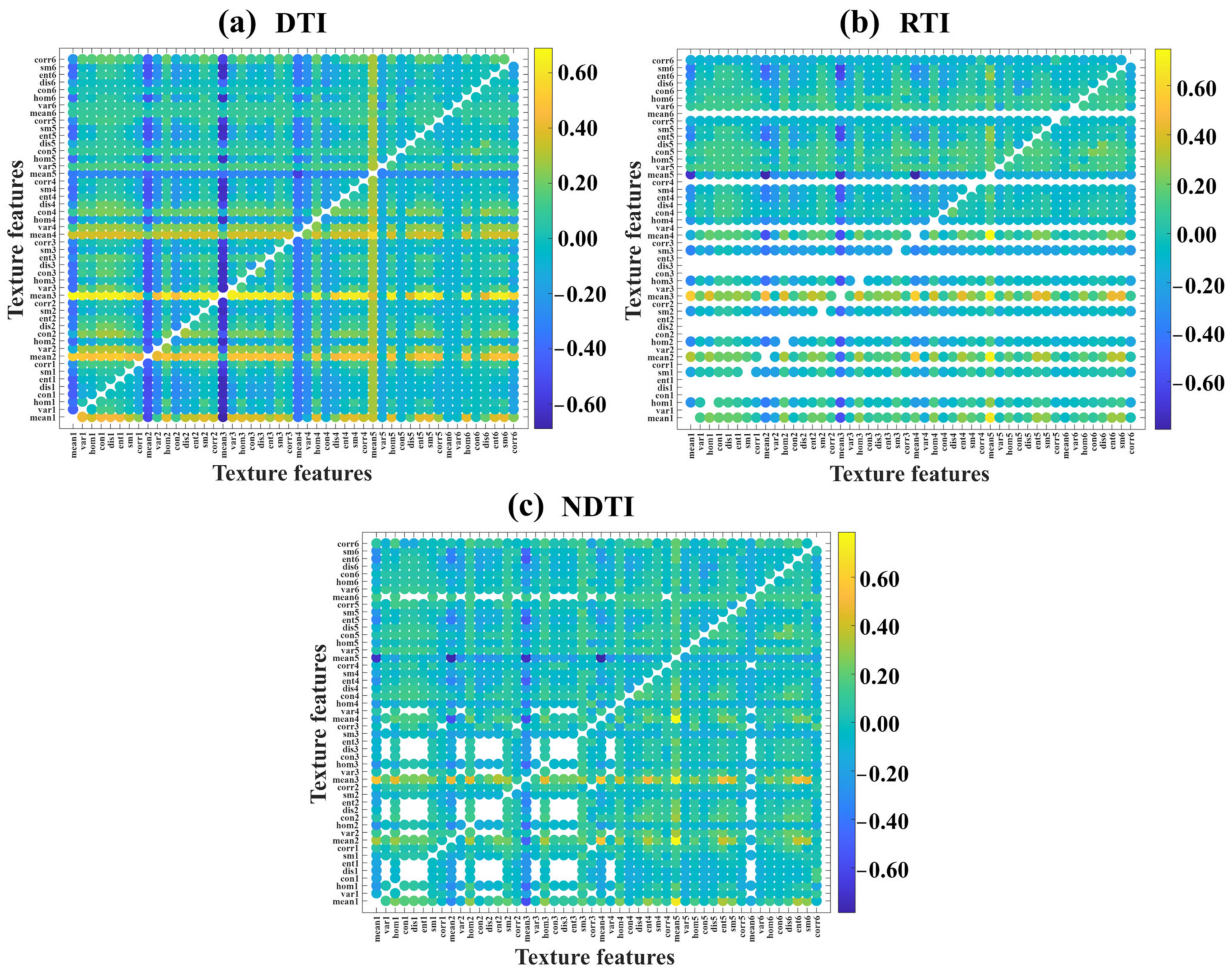
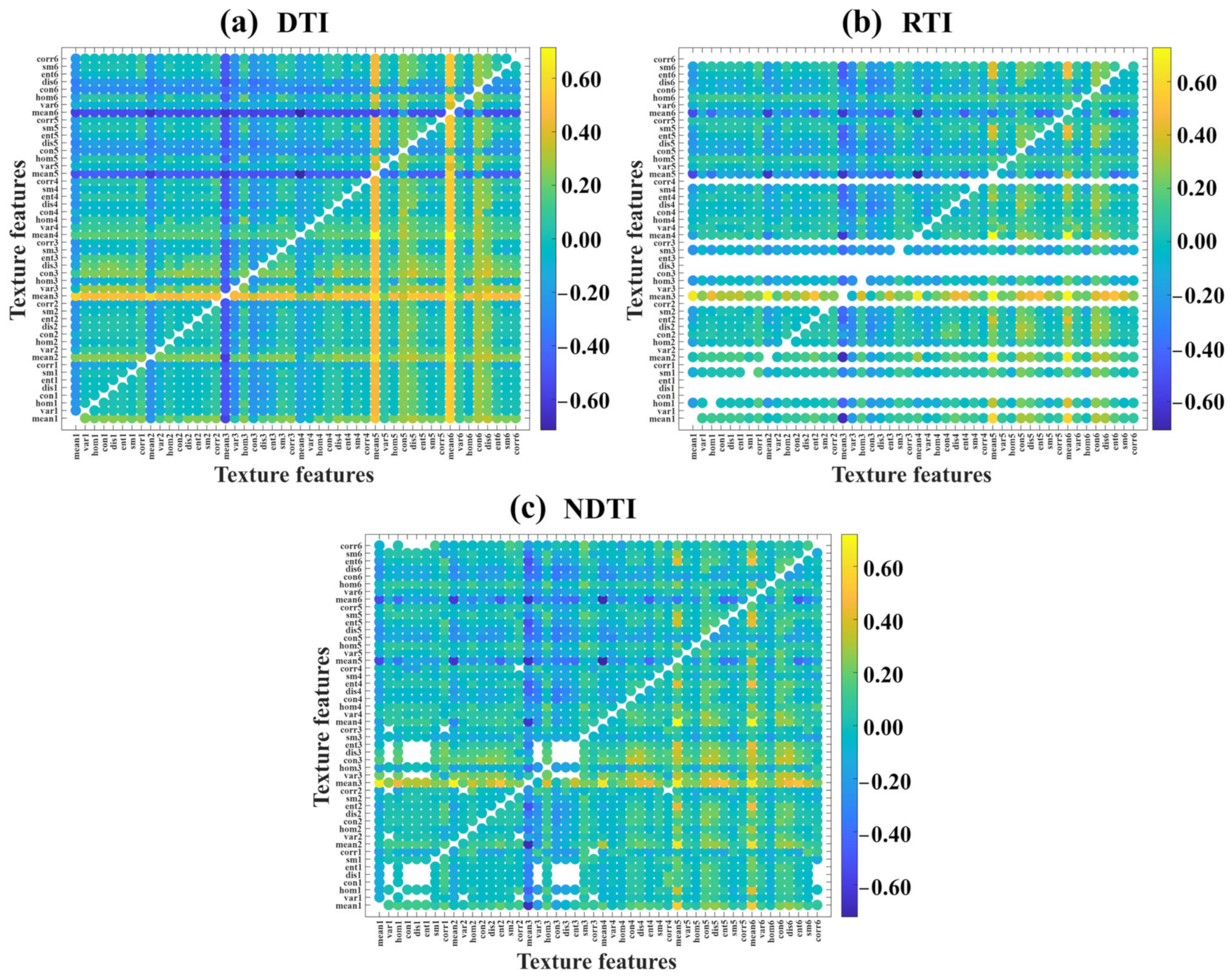
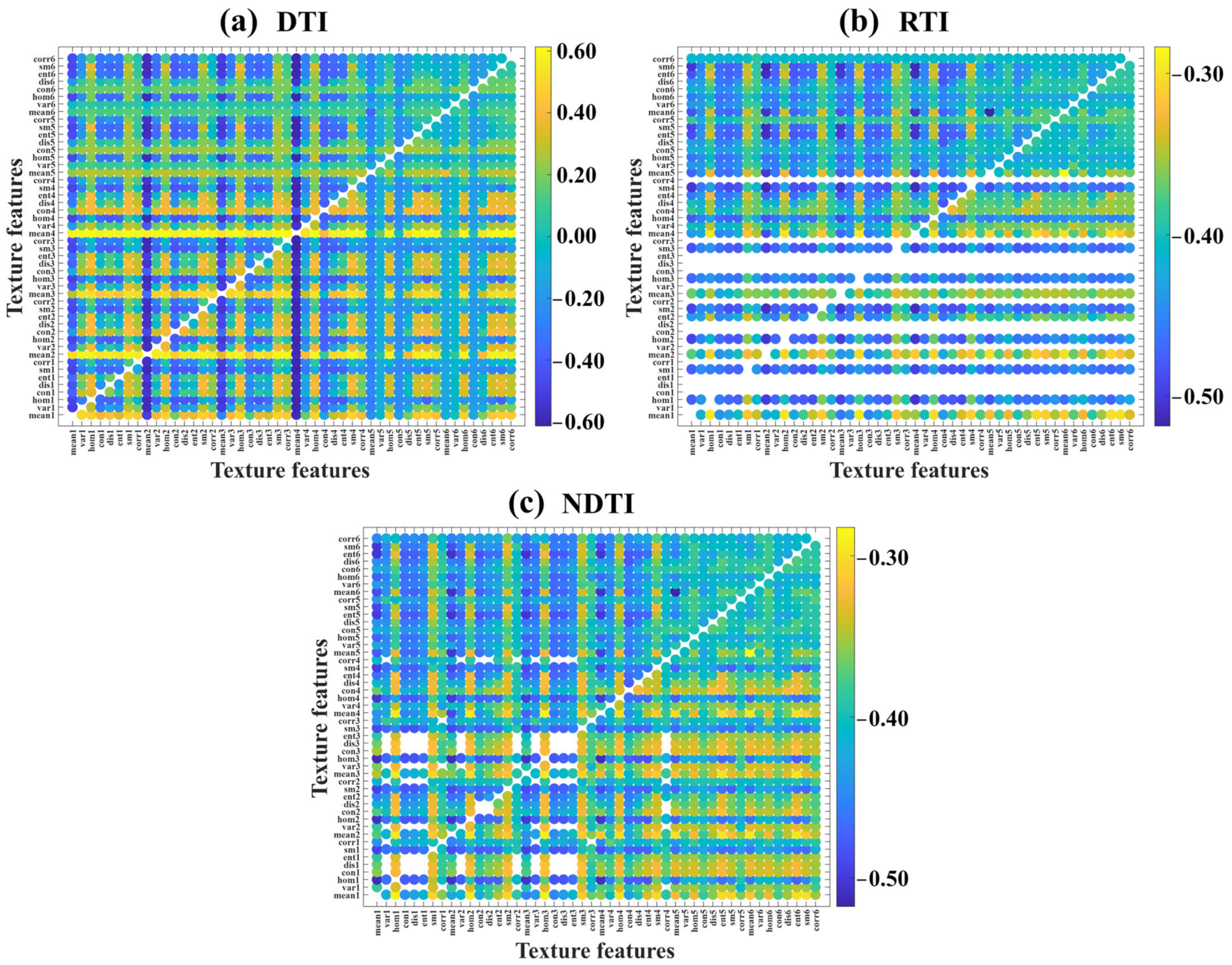
3.2.1. Selection of Optimal TIs

The correlation between individual texture features and RCCC was relatively weak. As shown in

Table 5. The correlation coefficient between texture features and RCCC.

Stages	Texture Feature	Correlation Coefficient (r)
		Blue	Green	Red	RE720	RE750	NIR
Heading	Mean (mean)	−0.32 **	−0.39 **	−0.38 **	−0.42 **	−0.17	−0.07
	Variance (var)	−0.14	−0.22 *	−0.18	−0.16	−0.07	−0.03
	Homogeneity (hom)	0.24 *	0.22 *	0.22 *	0.27 **	0.06	0.12
	Contrast (con)	−0.20 *	−0.25 *	−0.15	−0.28 **	−0.21 *	−0.16
	Dissimilarity (dis)	−0.24 *	−0.24 *	−0.21 *	−0.29 **	−0.17	−0.16
	Entropy (ent)	−0.21 *	−0.26 **	−0.24 *	−0.27 **	−0.01	0.03
	Second moment (sm)	0.18	0.22 *	0.23 *	0.24 *	0.01	−0.03
	Correlation (corr)	0.02	−0.04	0.08	−0.06	−0.11	−0.01
Flowering	Mean (mean)	−0.32 **	−0.43 **	−0.54 **	−0.32 **	0.24 *	−0.03
	Variance (var)	0.03	−0.27 **	−0.09	−0.235 *	−0.15	−0.09
	Homogeneity (hom)	−0.05	0.10	−0.02	0.09	0.04	−0.02
	Contrast (con)	0.08	−0.23 *	−0.02	−0.17	−0.11	−0.03
	Dissimilarity (dis)	0.06	−0.15	0.01	−0.13	−0.08	−0.01
	Entropy (ent)	0.03	−0.02	−0.06	−0.05	0.01	−0.04
	Second moment (sm)	−0.02	0.03	0.02	0.05	0.03	0.06
	Correlation (corr)	−0.10	0.00	−0.03	−0.03	−0.12	−0.17
Filling	Mean (mean)	−0.23 *	−0.2 **	−0.48 **	−0.17	0.46 **	0.53 **
	Variance (var)	0.00	−0.09	−0.26 **	−0.10	0.05	0.08
	Homogeneity (hom)	−0.02	0.04	0.14	−0.08	−0.05	−0.07
	Contrast (con)	0.01	−0.02	−0.23 *	0.04	0.24 *	0.28 **
	Dissimilarity (dis)	0.02	−0.03	−0.19 *	0.07	0.19 *	0.22 *
	Entropy (ent)	0.02	−0.03	−0.13	−0.06	0.09	0.07
	Second moment (sm)	−0.01	0.03	0.11	0.07	−0.10	−0.04
	Correlation (corr)	0.13	0.09	0.04	−0.04	0.00	0.01

Note: ** indicates statistical significance at the 0.01 level (two-tailed), and * indicates statistical significance at the 0.05 level (two-tailed).

, more than half of the selected texture features exhibited low correlations with RCCC. Only a tiny portion of the texture features moderately correlated with RCCC. Specifically, during the heading and flowering stages, the mean values of RE₇₂₀, green, red, and blue bands showed a moderate correlation with RCCC, with |r| values ranging from 0.32 to 0.54 (p < 0.01). During the filling stage, the mean values of the red, red-edge 2, and NIR bands correlated moderately with RCCC, with |r| values ranging from 0.46 to 0.53 (p < 0.01). In contrast, the |r| values for the remaining texture features ranged from 0.01 to 0.29, indicating poor correlation with RCCC.

Given the weak correlation between individual texture features and RCCC, their application in accurately predicting RCCC is limited. Therefore, this study utilized TIs composed of various texture features from different spectral bands, including DTI, RTI, and NDTI. Compared to individual texture features, the correlation between TIs and RCCC significantly improved. Figure 2, Figure A1 and Figure A2 illustrate the correlation between TIs, formed by arbitrary combinations of texture features from different bands, and RCCC. TIs with the highest correlation with RCCC were selected as independent variables for each growth stage. For the heading stage, the optimal TIs were DTI (corr_red, mean_RE₇₂₀), RTI (mean_RE₇₅₀, mean_NIR), and NDTI (mean_NIR, mean_RE₇₅₀), with |r| values of 0.61, 0.59, and 0.59, respectively. For the flowering stage, the optimal TIs were DTI (mean_blue, mean_red), RTI (mean_RE₇₂₀, mean_RE₇₅₀), and NDTI (mean_RE₇₅₀, mean_RE₇₂₀), with |r| values of 0.69, 0.80, and 0.79, respectively. For the filling stage, the optimal TIs were DTI (mean_NIR, mean_RE₇₂₀), RTI (mean_RE₇₅₀, mean_RE₇₂₀), and NDTI (mean_RE₇₅₀, mean_RE₇₂₀), with |r| values of 0.72, 0.73, and 0.72, respectively. All selected optimal TIs were significantly correlated with RCCC at the 0.01 level.

3.2.2. Correlation Analysis Between VIs and RCCC

The relationship between 15 selected VIs and field-measured RCCC was evaluated using Pearson correlation analysis, with the results presented in

Table 6. The correlation coefficient between VIs and RCCC.

VIs	Heading	Flowering	Filling
NPCI	−0.46 **	−0.69 **	−0.65 **
VDVI	−0.36 **	−0.60 **	−0.63 **
NDVI	0.48 **	0.69 **	0.64 **
GNDVI	0.62 **	0.72 **	0.60 **
GCI	0.60 **	0.69 **	0.62 **
SR	0.51 **	0.69 **	0.70 **
MSR	0.48 **	0.69 **	0.64 **
RESR720	−0.32 **	−0.53 **	−0.58 **
RESR750	−0.42 **	−0.65 **	−0.62 **
LCI720	0.59 **	0.77 **	0.69 **
LCI750	0.65 **	0.73 **	0.50 **
NDRE720	0.61 **	0.78 **	0.70 **
NDRE750	0.65 **	0.69 **	0.36 **
RECI720	0.59 **	0.75 **	0.70 **
RECI750	0.65 **	0.69 **	0.35 **

Note: ** indicates statistical significance at the 0.01 level (two-tailed).

. The analysis revealed that all VIs exhibited significant correlations with RCCC (p < 0.01), with |r| values exceeding 0.35. Among the growth stages, indices such as GNDVI, GCI, SR, LCI₇₂₀, NDRE₇₂₀, and RECI₇₂₀ consistently demonstrated robust correlations with RCCC, achieving correlation coefficients above 0.50. Notably, NDRE displayed the highest correlation across all stages, with |r| consistently exceeding 0.60.

Conversely, specific indices, including VDVI, RESR₇₂₀, and RESR₇₅₀, showed weaker correlations with RCCC during the heading stage (|r| < 0.43), though their correlations improved significantly in the flowering and filling stages (|r| > 0.52). Additionally, NDRE₇₅₀ and RECI₇₅₀ exhibited strong correlations during the heading and flowering stages (|r| > 0.64) but showed reduced correlation strength during the filling stage (|r| < 0.37). These findings highlight the dynamic relationship between VIs and RCCC across growth stages, underscoring the importance of selecting stage-specific indices for accurate chlorophyll content estimation.

3.3. The Estimation of RCCC

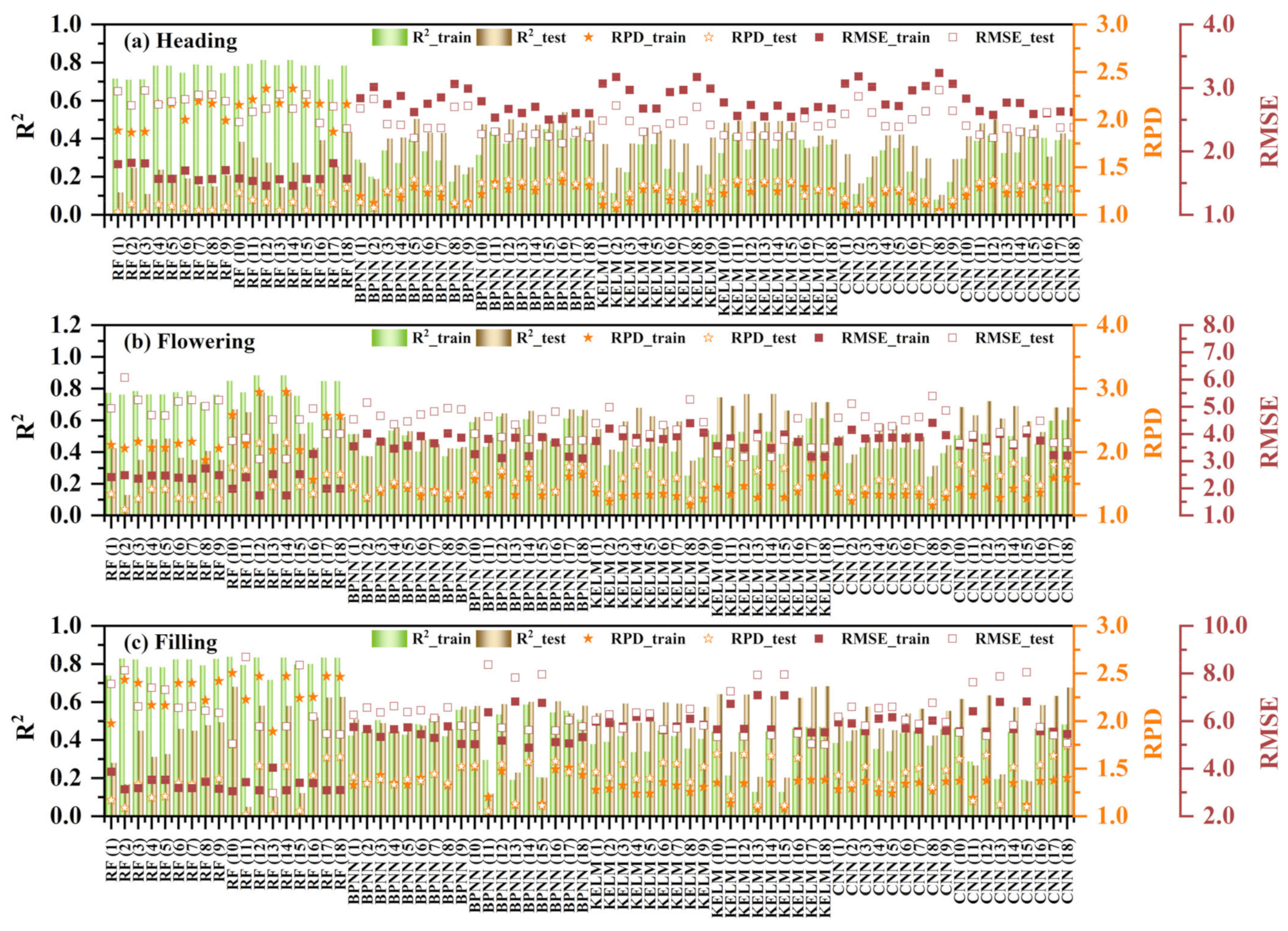
3.3.1. The Univariate Regression of RCCC

Figure 3 presents the univariate regression results for the eighteen parameters using four different algorithms, including fifteen VIs and three TIs. During the heading stage, the parameters with relatively better performance in the models were LCI₇₂₀, LCI₇₅₀, NDRE₇₂₀, RECI₇₂₀, DTI, RTI, and NDTI. However, the overall model performance was poor, with RPD values of less than 1.4. In the flowering stage, the better-performing indices included LCI₇₂₀, NDRE₇₂₀, RECI₇₂₀, RTI, and NDTI, with R² > 0.4 and RPD > 1.4. Among them, the RF model for LCI₇₂₀ (R²_train = 0.88, RPD_train = 2.95, R²_test = 0.78, and RPD_test = 2.15) and the RF model for NDRE₇₂₀ (R²_train = 0.88, RPD_train = 2.94, R²_test = 0.78, and RPD_test = 2.15) showed the best performance. During the filling stage, the indices with better model performance were LCI₇₂₀, NDRE₇₂₀, RECI₇₂₀, DTI, RTI, and NDTI, with R² > 0.4 and RPD > 1.4. The RF model for LCI₇₂₀ exhibited the best performance, with R²_train = 0.84, RPD_train = 2.51, R²_test = 0.68, and RPD_test = 1.75.

For univariate regression models, the RF model outperformed the other models in terms of training set fitting, with an average R²_train of 0.77. However, its R²_test significantly decreased and its RMSE increased for the testing set, suggesting the model may suffer from overfitting. The BP model performed better on the testing set, with an average R²_test of 0.47. Moreover, the difference in accuracy between the training and testing sets was smaller for the BP model compared to the other models, indicating stable performance across different datasets. In contrast, both the KELM and CNN models showed relatively low R² values on the training set, with an average R²_train of 0.37, indicating weaker fitting capability. Overall, the univariate models performed poorly in estimating RCCC during the heading stage, with low R² and RPD values. However, the model’s performance improved during the flowering and filling stages, with increased R² and RPD values. Among the four model algorithms, RF and BP models demonstrated stronger fitting capabilities, while KELM and CNN models performed poorly in fitting the training data.

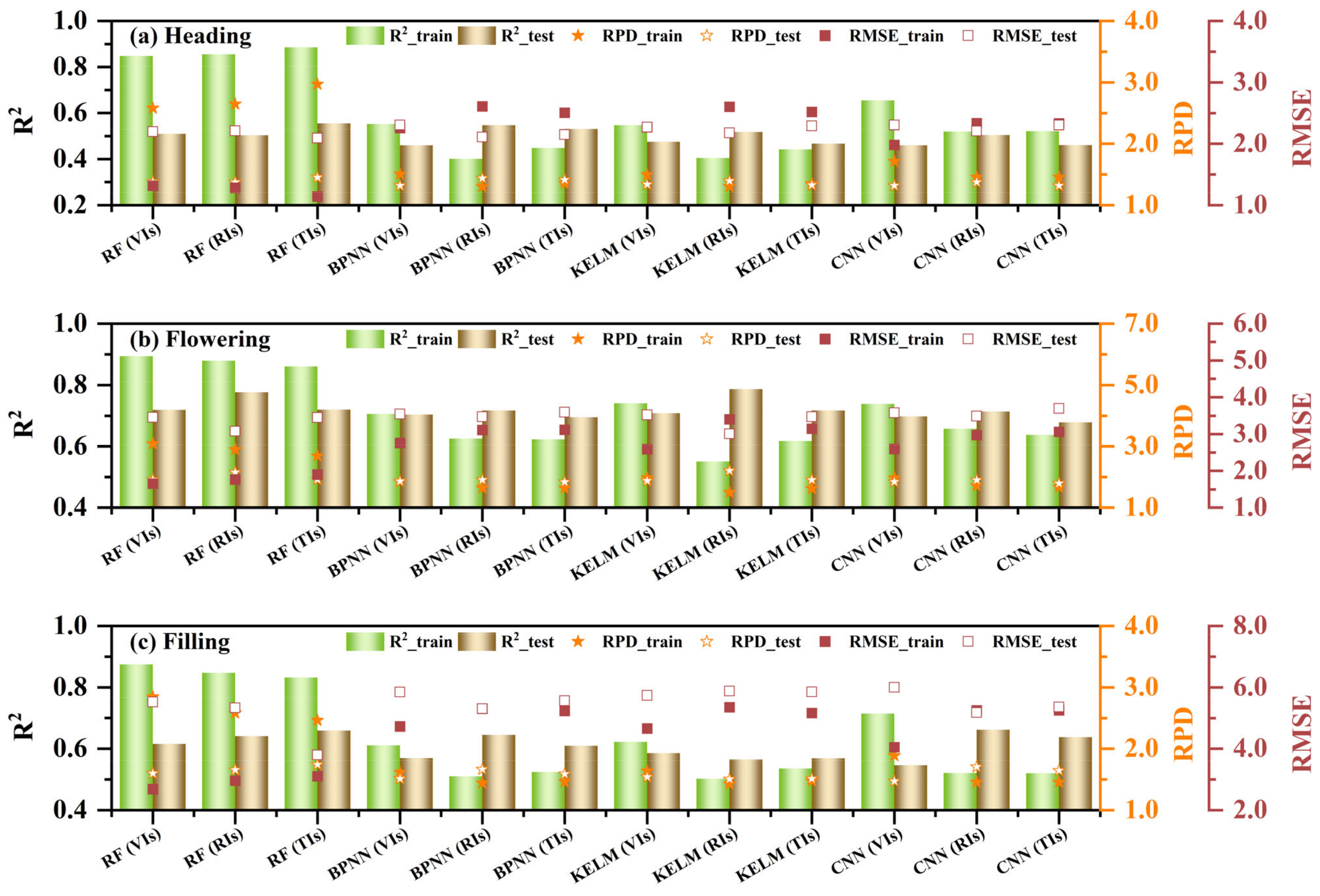
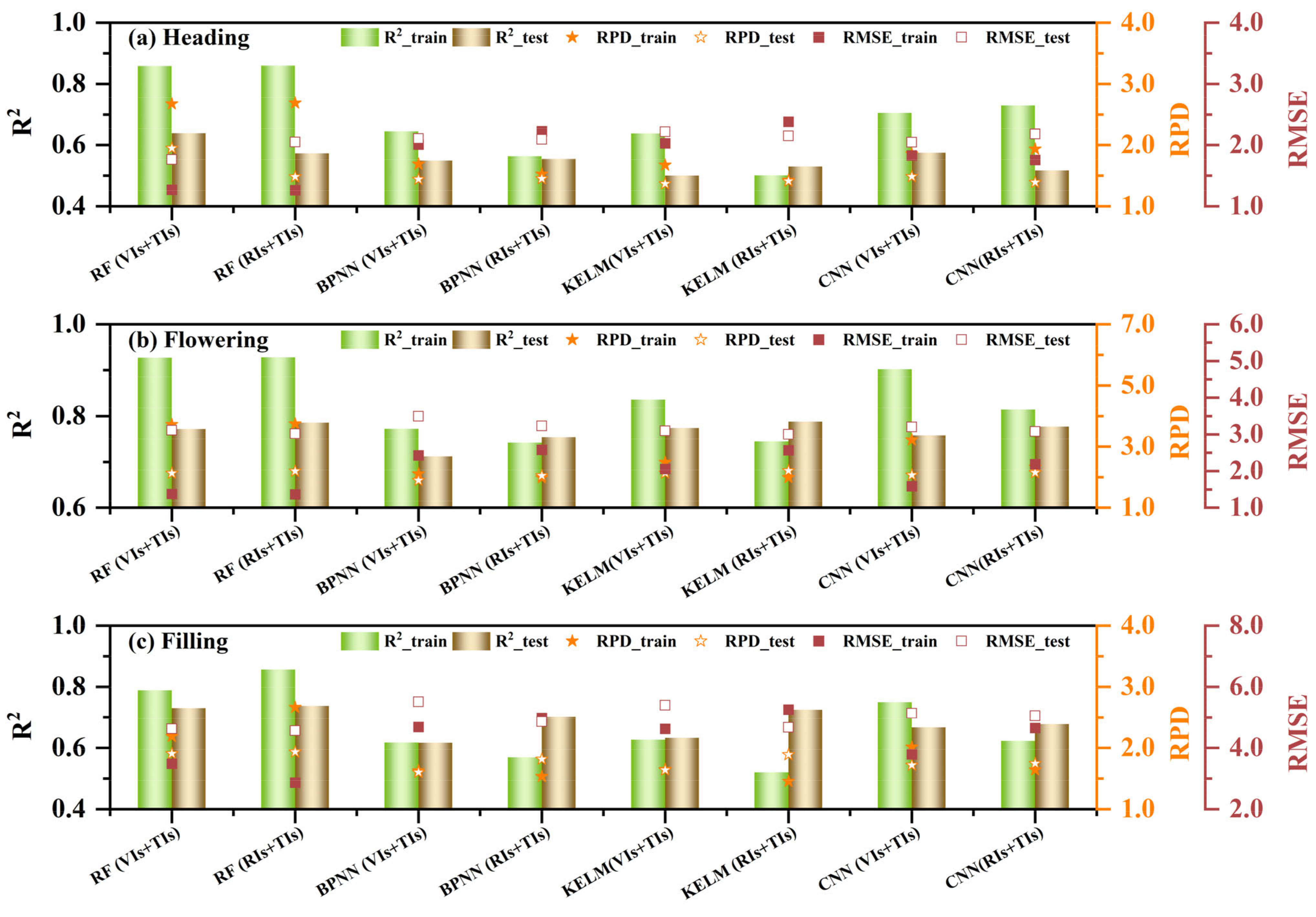
3.3.2. The Multivariate Regression of RCCC

Based on univariate regression analysis and correlation analysis, it was found that LCI₇₂₀, NDRE₇₂₀, and RECI₇₂₀ are the three most prominent RIs. In this study, fifteen vegetation indices and three texture vegetation indices were selected as independent variables, with these three prominent RIs also used as independent variables. Four regression algorithms were applied to construct regression models, aiming to explore the differences in regression performance with different combinations of independent variables, as well as to compare the performance differences between multiple regression and univariate regression. The results are shown in Figure 4 and Figure 5.

For models based on VIs, during the heading stage, all models performed poorly on the testing set (RPD_test < 1.4). The RF model achieved the best performance in fitting the data, with R²_train = 0.85, RPD_train = 2.58, R²_test = 0.51, and RPD_test = 1.38. The CNN model ranked second, with R²_train = 0.65, RPD_train = 1.71, R²_test = 0.46, and RPD_test = 1.32. KELM outperformed BPNN slightly in this stage. During the flowering stage, all models reasonably estimated RCCC (RPD > 1.8), with the RF model performing the best (R²_train = 0.89, RPD_train = 3.08, R²_test = 0.72, and RPD_test = 1.92). The performance of other models on the testing set ranked as KELM > BPNN > CNN. During the filling stage, all models achieved rough estimates of RCCC (1.4 < RPD < 1.8), with RF leading, indicated by R²_train = 0.87, RPD_train = 2.84, R²_test = 0.62, and RPD_test = 1.60, while other models ranked KELM > BPNN > CNN in terms of testing set performance.

For the models based on RIs, during the heading stage, the overall model performance was relatively poor. Among them, RF model showed the best fitting performance on the training set (R²_train = 0.86, RPD_train = 2.64). However, the CNN provided a more balanced performance overall, with R²_train = 0.52, RPD_train = 1.45, R²_test = 0.50, and RPD_test = 1.37. During the flowering stage, RF had the best overall performance, with R²_train = 0.88, RPD_train = 2.89, R²_test = 0.78, and RPD_test = 2.15. The performance of other models on the testing set ranked as KELM > RF > BP > CNN. During the filling stage, RF led with the best model outcomes, showing R²_train = 0.85, RPD_train = 2.58, R²_test = 0.64, and RPD_test = 1.66, while the R²_train values of the other models were all less than 0.55, indicating poorer fitting performance.

For models based on TIs, during the heading stage, the RF model achieved the best performance in estimating RCCC, with R²_train = 0.89, RPD_train = 2.97, R²_test = 0.55, and RPD_test = 1.45. The performance of other models was poor, with RPD values below 1.4, indicating weaker fitting ability. During the flowering stage, RF exhibited the best model performance, marked by R²_train = 0.86, RPD_train = 2.69, R²_test = 0.72, and RPD_test = 1.92. Other models had RPD values below 1.7 for the training set, suggesting poor fitting performance. During the filling stage, RF led with the best performance, reaching R²_train = 0.83, RPD_train = 2.46, R²_test = 0.66, and RPD_test = 1.74. The performance of other models was, again, suboptimal, with RPD values on the training set below 1.5, indicating poor fitting ability.

For models based on VIs + TIs, during the heading stage, the RF model exhibited the best fitting performance, achieving an R²_train of 0.86, RPD_train of 2.67, R²_test of 0.64, and RPD_test of 1.95. Other models ranked as CNN > BPNN > KELM, with KELM showing an RPD_test of less than 1.4, indicating poor estimation accuracy. During the flowering stage, all models performed well (RPD > 2.0), with RF exhibiting the best model performance (R²_train = 0.93, RPD_train = 3.72, R²_test = 0.77, and RPD_test = 2.13). The other models ranked in fitting performance as follows: KELM > CNN > BPNN. For the filling stage, all models were able to roughly estimate RCCC (1.4 < RPD < 1.8), with RF providing the best fitting performance (R²_train = 0.79, RPD_train = 2.19, R²_test = 0.73, and RPD_test = 1.91), and the remaining models followed the order CNN > KELM > BPNN.

For the models based on RIs + TIs, during the heading stage, RF provided the best estimation, marked by R²_train = 0.86, RPD_train = 2.69, R²_test = 0.57, and RPD_test = 1.48, with the performance of the other models ranked as BPNN > KELM > CNN on the testing set. During the flowering stage, given that R² > 0.74 and RPD > 2.0, all models performed well, with RF showing an absolute fitting advantage, presenting R²_train = 0.93, RPD_train = 3.74, R²_test = 0.79, and RPD_test = 2.20. During the filling stage, RF again demonstrated the best fitting performance, with R²_train = 0.86, RPD_train = 2.66, R²_test = 0.74, and RPD_test = 1.93. The accuracy differences between datasets for other models are ranked from smallest to largest as follows: CNN > BPNN > KELM.

Compared to models using VIs as independent variables, the models based on RIs showed improvements in fit performance on the testing set ranging from 1.80% to 21.12% (except for RF during the heading stage and KELM during the filling stage), and no significant advantages were observed on the training set. Models using VIs + TIs as independent variables outperformed those using only VIs on the testing set, with R²_test improvements ranging from 1.17% to 24.93% and RPD_test improvements from 1.42% to 19.34% across all stages. Similarly, models using VIs + TIs also performed better than those using TIs alone, with R²_test increases of 1.21% to 24.76% and RPD_test increases of 0.96% to 15.89%. Additionally, models using RIs + TIs outperformed those using RIs alone, with R² increasing by 0.16% to 40.70% and RPD increasing by 0.30% to 46.42%. Overall, models utilizing RIs + TIs also demonstrated superior performance compared to those using TIs alone, with R² improving by 2.91% to 39.83% and RPD improving by 2.72% to 39.72%, except for KELM during the filling stage and RF during the heading stage. Thus, combining vegetation indices and texture indices for estimating RCCC can effectively enhance the estimation accuracy. Compared to models with VIs + TIs, the models using RIs + TIs generally exhibited an overall improvement in testing performance ranging from 0.98% to 14.43%, with reasonable training performance but no significant advantages, indicating that the use of RIs+TIs for estimating RCCC holds potential.

4. Discussion

4.1. Analysis of Univariate Regression and Outstanding Variable

Univariate regression in machine learning can quantify the influence of individual independent variables on a target variable, helping to identify the independent contribution of each variable and providing a basis for feature selection and model optimization [52]. If a complex model performs exceptionally well in univariate regression tasks, it indicates potential applicability, thus validating its potential for further enhancement and application in multivariate problems. In this study, the univariate regression analysis of vegetation indices revealed that the LCI₇₂₀, including the red-edge band, exhibited strong performance during the heading, flowering, and filling stages. Additionally, two other red-edge vegetation indices (NDRE₇₂₀ and RECI₇₂₀) and three texture vegetation indices (DTI, RTI, and NDTI) demonstrated outstanding inversion capabilities, particularly during the flowering and filling stages. The excellent performance of these red-edge indices suggests that the red-edge spectrum centered around the 720 nm band is highly sensitive to variations in plant chlorophyll content. Numerous studies have shown that the red-edge band is situated in the transition zone between red and NIR light, reflecting subtle differences in chlorophyll absorption spectra, especially during periods of high chlorophyll content, such as flowering and filling stages [53]. For example, the research by Delegido et al. [54] confirmed the high sensitivity of the red-edge band, noting that red-edge-related vegetation indices (such as NAOC and NDI) significantly enhance the accuracy of chlorophyll content estimation. Furthermore, Clevers and Gitelson [55] found that red-edge indices (like RECI and MTCI) are particularly effective in estimating chlorophyll and nitrogen content in crop and grassland canopies through Sentinel-2 and Sentinel-3 data analyses. Moreover, given that image texture is highly sensitive to spatial heterogeneity [56], texture features may provide insights into canopy structural changes during the complex flowering and filling stages, thereby enhancing sensitivity to chlorophyll content. For instance, Yang et al. [57] demonstrated that differences in canopy structure affect the accuracy of chlorophyll content estimates, and integrating texture features can further improve the performance of predictive models.

The significance of red-edge vegetation and texture parameters in estimating chlorophyll content in winter wheat highlights the advantages of drones equipped with multispectral sensors for chlorophyll inversion. In this study, LCI₇₂₀ consistently demonstrated stable and excellent performance across different growth stages. However, it is necessary to note that the best-performing vegetation indices may vary across different studies, and a single index may not comprehensively reflect crop growth conditions. Therefore, to estimate chlorophyll content in winter wheat more accurately, it is crucial to combine multiple indices for a reasonable comprehensive analysis [14].

4.2. Improvement of RCCC Estimation Through Multivariate Regression and Texture Indices

Multivariate regression using machine learning algorithms can simultaneously consider multiple feature variables, capturing more complex relationships and thereby enhancing the predictive accuracy and robustness of models compared to univariate regression [58]. In this study, compared to the optimal univariate regression models, the R² values of the preeminent multivariate regression increased by 0.35% to 69.55%. This indicates that increasing the number of features generally benefits the established regression models, improving the estimation of canopy chlorophyll content in winter wheat, which is similar to the results of Wang et al. [14]. The improvement may stem from introducing additional feature variables, such as red-edge band indices and texture features, which allow the model to capture more latent information related to chlorophyll content, thus enhancing its generalization capability [59,60]. For instance, Sun et al. [61] found that using a combination of various vegetation indices yielded better results with the random forest model for estimating chlorophyll content in winter wheat compared to single-index models, demonstrating a significant performance improvement. Additionally, Yang et al. [57] noted that incorporating texture features alongside vegetation indices (MSR, RVI, and NDVI) significantly enhanced the accuracy of chlorophyll estimations.

Texture indices can capture the significant physiological changes that occur in crops during different growth stages, thereby enhancing the accuracy of chlorophyll content estimation [62]. In this study, several texture indices demonstrated strong correlations with RCCC: during the heading stage, DTI (corr_red, mean_RE₇₂₀), RTI (mean_RE₇₅₀, mean_NIR), and NDTI (mean_NIR, mean_RE₇₅₀); during the flowering stage, DTI (mean_blue, mean_red), RTI (mean_RE₇₂₀, mean_RE₇₅₀), and NDTI (mean_RE₇₅₀, mean_RE₇₂₀); and during the filling stage, DTI (mean_NIR, mean_RE₇₂₀), RTI (mean_RE₇₅₀, mean_RE₇₂₀), and NDTI (mean_RE₇₅₀, mean_RE₇₂₀). The |r| ranged from 0.59 to 0.80 (p < 0.01). The correlation of texture measurement is utilized to measure the similarity between pixels within an image, aiding in capturing spatial structural characteristics [63]. The mean of texture measurements encompasses the average values of the target and background within a moving window, a method that effectively smooths the image and mitigates the influence of background noise on estimation results [64]. Additionally, the strong absorption of green vegetation in the red and blue bands, coupled with high reflectance in the NIR band as a result of the canopy structure, along with the heightened sensitivity of the red-edge band to leaf health and physiological status, underscores the importance of these bands in estimating physiological parameters of vegetation [65,66,67]. By combining the mean values and correlation measurements from these bands, texture indices can enhance the expression of light absorption and reflection characteristics of vegetation, thus providing a more accurate representation of spatial changes in canopy structure [68].

In this study, integrating texture indices into the multivariate regression model based on vegetation indices led to a notable increase of 0.16% to 40.70% in R ² values for some models. This indicates that incorporating texture indices effectively enhances the estimation of canopy chlorophyll content in winter wheat, aligning with the findings of Yu et al. [69]. Furthermore, several other studies have corroborated the positive impact of texture indices. For instance, research conducted by Wang et al. [22] demonstrated that combining VIs with TIs significantly improves the accuracy of SPAD estimates across all growth stages of rice compared to using VIs alone. Similarly, Zheng et al. [70] found that integrating the texture index (NDTI) with vegetation indices markedly enhances the accuracy of biomass estimations in rice compared to using vegetation indices in isolation. Additionally, Zhang et al. [71] reported that combining spectral features and texture indices (such as NDTI or DTI) yields better estimation results than relying solely on spectral or texture features.

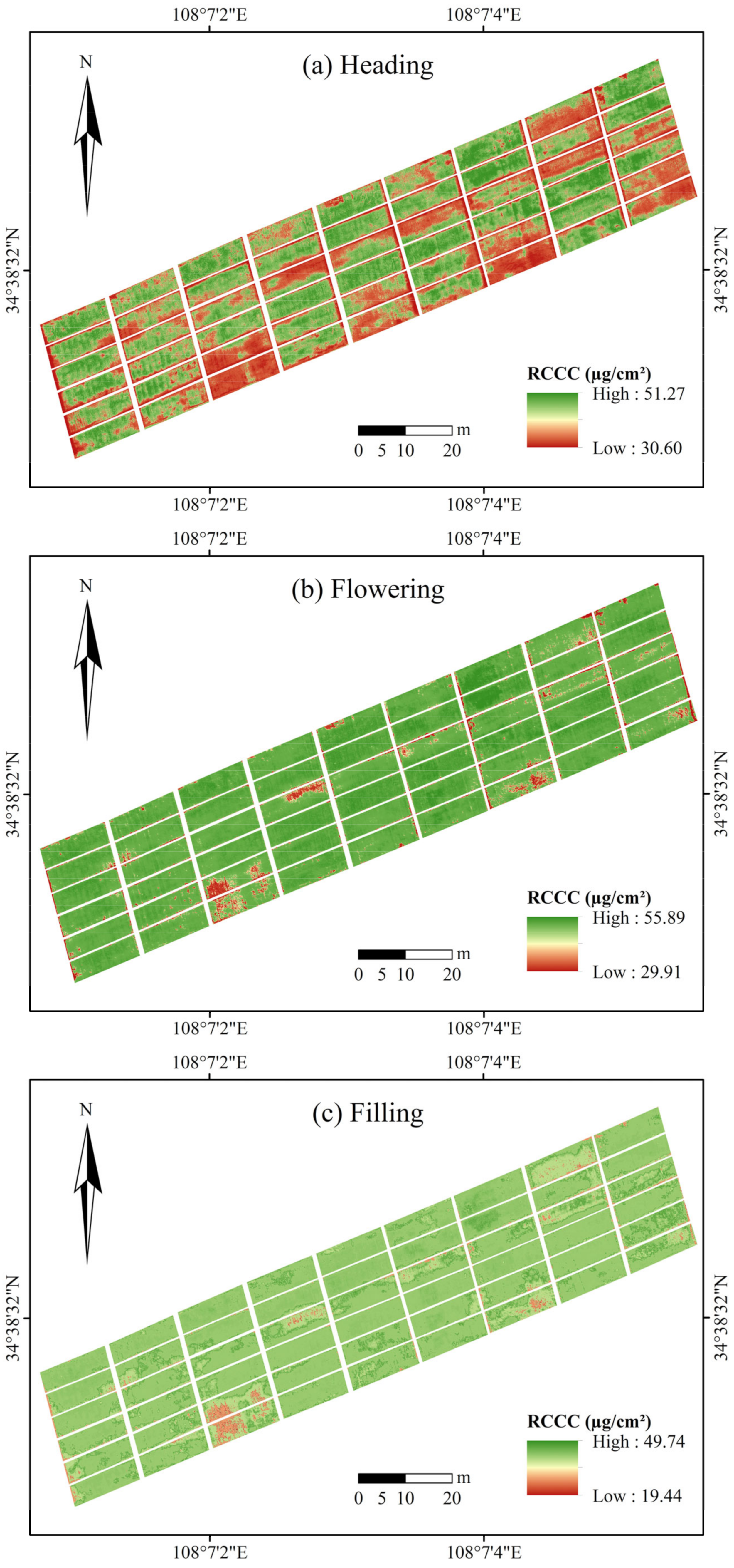
4.3. Model Adaptability and Optimal Mapping of RCCC

Among the models evaluated, the RF model exhibited exceptional performance but showed a high risk of overfitting in univariate regression during the heading stage, particularly under weak correlations and limited data. This vulnerability likely arises from its flexible feature selection, making it susceptible to data noise-reducing generalization capability [72]. The BPNN model demonstrated a relatively small performance difference between the training and testing sets in both univariate and multivariate regressions, indicating a certain degree of generalization ability. However, it performed poorly in the univariate regression during the heading stage, which may be attributed to the limited feature information provided by a single variable [73]. The CNN model demonstrated weak univariate regression performance, as it can only perform univariate regression when utilizing a regression layer, leading to results inferior to those of other algorithms, consistent with the findings of Zhao et al. [74]. This is primarily because convolution operations require multidimensional features for effective extraction, and multivariate regression captures more feature correlations through convolution, thus enhancing regression outcomes [75]. Additionally, the KELM model excelled in handling multidimensional features, outperforming univariate regression due to its adaptability and strong fitting capability for high-dimensional data [76].

Comparing all model performances across different stages, the RF model based on VIS+TIS performed best during the heading stage, evidenced by R²_train = 0.86, RPD_train = 2.67, R²_test = 0.64, and RPD_test = 1.95. During the flowering stage, the RF model based on RIs+TIs excelled, with R²_train = 0.93, RPD_train = 3.74, R²_test = 0.79, and RPD_test = 2.20. In the filling stage, the RF model based on RIs+TIs again showed the best performance, with R²_train = 0.86, RPD_train = 2.66, R²_test = 0.74, and RPD_test = 1.93. Using image matrices and well-trained Python models, spatial distribution maps of winter wheat canopy chlorophyll content during the growth stages were generated (Figure 6). During the heading stage, winter wheat transitions from vegetative to reproductive growth, achieving peak photosynthesis with maximum leaf area and high canopy chlorophyll content, with the average RCCC around 41.63. However, the impact of previously cultivated nutrient levels is significant, with visibly poorer canopy leaf growth and lower chlorophyll content in areas without or with minimal nitrogen fertilization, where RCCC values typically range between 30.60 and 39.96. Additionally, RCCC is generally lower along the edges of plots, likely influenced by uneven fertilization leading to slower canopy leaf growth. During the flowering stage, the canopy structure stabilizes, and photosynthesis remains high, maintaining elevated chlorophyll levels with an average RCCC of around 42.89. However, as older leaves begin to age, the lower values of RCCC decline slightly, particularly in areas with less nitrogen application and disease stress, where leaf health progressively deteriorates, and the RCCC values are primarily between 29.91 and 36.40. In the filling stage, as leaves age, the diminishing size and health of the leaves impact the efficiency of photosynthesis, causing the leaf color to yellow and chlorophyll content to decrease, with an average RCCC of about 32.98. The inversion map matches the actual growth conditions, further confirming the feasibility of remote sensing inversion.

4.4. Limitations and Future Perspectives

This study underscored the critical role of red-edge vegetation indices (LCI₇₂₀, NDRE₇₂₀, RECI₇₂₀) and texture indices (DTI, RTI, NDTI) in estimating winter wheat chlorophyll content, highlighting their relevance in improving model accuracy. While the integration of multispectral data offered a high-resolution, non-destructive approach to agricultural monitoring, the study was constrained by certain limitations. First, research on the spectral characteristics of red-edge vegetation indices was limited, and integrating hyperspectral data was necessary to further refine the study of these indices, which could potentially enhance the sensitivity and accuracy of chlorophyll estimation. Second, the feature selection introduced potential subjectivity, and the sensitivity of texture index calculations to parameter choices, such as window size, requires further optimization. Additionally, the use of UAV imagery, despite its precision, was limited in spatial coverage, necessitating further validation through satellite integration for large-scale applications. Future research should combine hyperspectral and satellite data to enhance model performance, validate models under diverse conditions for winter wheat, and employ advanced machine learning techniques, such as hybrid neural networks, to capture complex interactions. These advancements will not only help reduce costs but will also improve the scalability and effectiveness of winter wheat monitoring and management.

5. Conclusions

This study analyzed the capability of spectral and textural indices derived from UAV multispectral images to estimate the canopy chlorophyll content in winter wheat. The main conclusions are as follows:

(1)

Vegetation indices based on red-edge bands with high sensitivity (LCI₇₂₀, NDRE₇₂₀, RECI₇₂₀) and texture indices with multi-spatial information (DTI, RTI, NDTI) were critical in estimating RCCC. Univariate regression models were reasonable for the flowering and filling stages, while the outstanding multivariate models, which incorporate multiple features, captured more complex relationships and outperformed univariate models, achieving an R² increase of 0.35% to 69.55% compared to the optimal univariate models.

(2)

The RF model demonstrated outstanding performance in both univariate and multivariate regressions. Among all models, the RF model based on RIS+TIS during the flowering stage exhibited the best performance (R²_train = 0.93, RMSE_train = 1.36, RPD_train = 3.74, R²_test = 0.79, RMSE_test = 3.01, RPD_test = 2.20). With more variables, BPNN, KELM, and CNN models better leverage the advantages of neural networks, thus improving training performance.

(3)

Compared to using single-type features for RCCC estimation, the combination of vegetation indices and texture indices increased from 0.16% to 40.70% in the R² values of some models. Integrating spectral and texture information from UAV multispectral images effectively estimates the RCCC of winter wheat in this study area, providing valuable information for winter wheat management. However, future work should expand the applicability of the estimation models developed in this study.

References

1. Khaledi-Alamdari, M.; Majnooni-Heris, A.; Fakheri-Fard, A.; Russo, A. Probabilistic climate risk assessment in rainfed wheat yield: Copula approach using water requirement satisfaction index. Agric. Water Manag. 2023, 289, 108542. [Google Scholar] [CrossRef]
2. Korotkova, I.V.; Chaika, T.O.; Romashko, T.P.; Chetveryk, O.O.; Rybalchenko, A.M.; Barabolia, O.V. Emmer wheat productivity formation depending on pre-sowing seed treatment method in organic and traditional technology cultivation. Regul. Mech. Biosyst. 2023, 14, 41–47. [Google Scholar] [CrossRef]
3. Hema, K.; Yogita, N.; Nitin, D.; Swapna, C. Design of Spectral Absorbance-Based Electronic Reader for Chlorophyll Measurement. SSRG Int. J. Electr. Electron. Eng. 2023, 10, 46–55. [Google Scholar] [CrossRef]
4. Cartelat, A.; Zoran, G.C.; Goulas, Y.; Sylvie, M.; Caroline, L.; Prioul, J.L.; Aude, B.; Jeuffroy, M.H.; Philippe, G.; Giovanni, A.; et al. Optically assessed contents of leaf polyphenolics and chlorophyll as indicators of nitrogen deficiency in wheat (Triticum aestivum L.). Field Crops Res. 2005, 91, 35–49. [Google Scholar] [CrossRef]
5. Goulas, Y.; Zoran, G.C.; Cartelat, A.; Moya, I. Dualex: A new instrument for field measurements of epidermal ultraviolet absorbance by chlorophyll fluorescence. Appl. Opt. 2004, 43, 4488–4496. [Google Scholar] [CrossRef]
6. Li, Z.; Wang, J.; He, P.; Zhang, Y.; Liu, H.; Chang, H.; Xu, X. Modelling of crop chlorophyll content based on Dualex. Trans. Chin. Soc. Agric. Eng. 2015, 31, 191–197. [Google Scholar]
7. Raffaele, C.; Fabio, C.; Simone, P.; Stefano, P. Chlorophyll estimation in field crops: An assessment of handheld leaf meters and spectral reflectance measurements. J. Agric. Sci. 2015, 153, 876–890. [Google Scholar] [CrossRef]
8. Liu, Y.; Wang, J.; Xiao, Y.; Shi, X.; Zeng, Y. Diversity Analysis of Chlorophyll, Flavonoid, Anthocyanin, and Nitrogen Balance Index of Tea Based on Dualex. Phyton-Int. J. Exp. Bot. 2021, 90, 1549–1558. [Google Scholar] [CrossRef]
9. Zhang, Z.; Zhu, L. A Review on Unmanned Aerial Vehicle Remote Sensing: Platforms, Sensors, Data Processing Methods, and Applications. Drones 2023, 7, 398. [Google Scholar] [CrossRef]
10. Qi, H.; Bingyu, Z.; Zeyu, W.; Liang, Y.; Jianwen, L.; Leidi, W.; Tingting, C.; Yubin, L.; Lei, Z. Estimation of Peanut Leaf Area Index from Unmanned Aerial Vehicle Multispectral Images. Sensors 2020, 20, 6732. [Google Scholar] [CrossRef]
11. Luo, S.; Jiang, X.; He, Y.; Li, J.; Jiao, W.; Zhang, S.; Xu, F.; Han, Z.; Sun, J.; Yang, J.; et al. Multi-dimensional variables and feature parameter selection for aboveground biomass estimation of potato based on UAV multispectral imagery. Front. Plant Sci. 2022, 13, 948249. [Google Scholar] [CrossRef] [PubMed]
12. Lu, N.; Wang, W.; Zhang, Q.; Li, D.; Yao, X.; Tian, Y.; Zhu, Y.; Cao, W.; Baret, F.; Liu, S.; et al. Estimation of Nitrogen Nutrition Status in Winter Wheat From Unmanned Aerial Vehicle Based Multi-Angular Multispectral Imagery. Front. Plant Sci. 2019, 10, 1601. [Google Scholar] [CrossRef] [PubMed]
13. Zhang, C.; Yi, Y.; Wang, L.; Zhang, X.; Chen, S.; Su, Z.; Zhang, S.; Xue, Y. Estimation of the Bio-Parameters of Winter Wheat by Combining Feature Selection with Machine Learning Using Multi-Temporal Unmanned Aerial Vehicle Multispectral Images. Remote Sens. 2024, 16, 469. [Google Scholar] [CrossRef]
14. Wang, W.; Cheng, Y.; Ren, Y.; Zhang, Z.; Geng, H. Prediction of Chlorophyll Content in Multi-Temporal Winter Wheat Based on Multispectral and Machine Learning. Front. Plant Sci. 2022, 13, 896408. [Google Scholar] [CrossRef]
15. Wang, Y.; Lola, S.; Poblete, T.; Victoria, G.-D.; Dongryeol, R.; Pablo, J.Z.T. Evaluating the role of solar-induced fluorescence (SIF) and plant physiological traits for leaf nitrogen assessment in almond using airborne hyperspectral imagery. Remote Sens. Environ. 2022, 279, 113141. [Google Scholar] [CrossRef]
16. Yue, J.; Yang, G.; Li, C.; Li, Z.; Wang, Y.; Feng, H.; Xu, B. Estimation of Winter Wheat Above-Ground Biomass Using Unmanned Aerial Vehicle-Based Snapshot Hyperspectral Sensor and Crop Height Improved Models. Remote Sens. 2017, 9, 708. [Google Scholar] [CrossRef]
17. Zhang, A.; Yin, S.; Wang, J.; He, N.; Chai, S.; Pang, H. Grassland Chlorophyll Content Estimation from Drone Hyperspectral Images Combined with Fractional-Order Derivative. Remote Sens. 2023, 15, 5623. [Google Scholar] [CrossRef]
18. Qian, B.; Ye, H.; Huang, W.; Xie, Q.; Pan, Y.; Xing, N.; Ren, Y.; Guo, A.; Jiao, Q.; Lan, Y. A sentinel-2-based triangular vegetation index for chlorophyll content estimation. Agric. For. Meteorol. 2022, 13, 925986. [Google Scholar] [CrossRef]
19. Ma, Y.; Ma, L.; Zhang, Q.; Huang, C.; Yi, X.; Chen, X.; Hou, T.; Lv, X.; Zhang, Z. Cotton Yield Estimation Based on Vegetation Indices and Texture Features Derived From RGB Image. Front. Plant Sci. 2019, 166, 105026. [Google Scholar] [CrossRef]
20. Liu, Y.; Liu, S.; Li, J.; Guo, X.; Wang, S.; Lu, J. Estimating biomass of winter oilseed rape using vegetation indices and texture metrics derived from UAV multispectral images. Comput. Electron. Agric. 2024, 14, 1265. [Google Scholar] [CrossRef]
21. Li, W.; Pan, K.; Liu, W.; Xiao, W.; Ni, S.; Shi, P.; Chen, X.; Li, T. Monitoring Maize Canopy Chlorophyll Content throughout the Growth Stages Based on UAV MS and RGB Feature Fusion. Agriculture 2024, 14, 1265. [Google Scholar] [CrossRef]
22. Wang, Y.; Tan, S.; Jia, X.; Qi, L.; Liu, S.; Lu, H.; Wang, C.; Liu, W.; Zhao, X.; He, L.; et al. Estimating Relative Chlorophyll Content in Rice Leaves Using Unmanned Aerial Vehicle Multi-Spectral Images and Spectral–Textural Analysis. Agronomy 2023, 13, 1541. [Google Scholar] [CrossRef]
23. Wang, T.; Gao, M.; Cao, C.; You, J.; Zhang, X.; Shen, L. Winter wheat chlorophyll content retrieval based on machine learning using in situ hyperspectral data. Comput. Electron. Agric. 2022, 193, 106728. [Google Scholar] [CrossRef]
24. Wang, Q.; Chen, X.; Meng, H.; Miao, H.; Jiang, S.; Chang, Q. UAV Hyperspectral Data Combined with Machine Learning for Winter Wheat Canopy SPAD Values Estimation. Remote Sens. 2023, 15, 4658. [Google Scholar] [CrossRef]
25. Feng, Z.; Guan, H.; Yang, T.; He, L.; Duan, J.; Song, L.; Wang, C.; Feng, W. Estimating the canopy chlorophyll content of winter wheat under nitrogen deficiency and powdery mildew stress using machine learning. Comput. Electron. Agric. 2023, 211, 107989. [Google Scholar] [CrossRef]
26. Cai, Y.L.; Yanying, M.; Hao, W.; Dan, W. Hyperspectral Estimation Models of Winter Wheat Chlorophyll Content Under Elevated CO2. Front. Plant Sci. 2021, 12, 642917. [Google Scholar] [CrossRef]
27. Liu, X.; Li, Z.; Xiang, Y.; Tang, Z.; Huang, X.; Shi, H.; Sun, T.; Yang, W.; Cui, S.; Chen, G.; et al. Estimation of Winter Wheat Chlorophyll Content Based on Wavelet Transform and the Optimal Spectral Index. Agronomy 2024, 14, 1309. [Google Scholar] [CrossRef]
28. Chen, X.; Li, F.; Shi, B.; Chang, Q. Estimation of Winter Wheat Plant Nitrogen Concentration from UAV Hyperspectral Remote Sensing Combined with Machine Learning Methods. Remote Sens. 2023, 15, 2831. [Google Scholar] [CrossRef]
29. Zoran, G.C.; Guillaume, M.; Naïma Ben, G.; Gwendal, L. A new optical leaf-clip meter for simultaneous non-destructive assessment of leaf chlorophyll and epidermal flavonoids. Physiol. Plant. 2012, 146, 251–260. [Google Scholar] [CrossRef]
30. Zhang, C.; Xue, Y. Estimation of Biochemical Pigment Content in Poplar Leaves Using Proximal Multispectral Imaging and Regression Modeling Combined with Feature Selection. Sensors 2023, 24, 217. [Google Scholar] [CrossRef]
31. Xue, J.; Su, B. Significant Remote Sensing Vegetation Indices: A Review of Developments and Applications. J. Sens. 2017, 2017, 1353691. [Google Scholar] [CrossRef]
32. Parida, P.K.; Somasundaram, E.; Krishnan, R.; Radhamani, S.; Sivakumar, U.; Parameswari, E.; Raja, R.; Shri Rangasami, S.R.; Sangeetha, S.P.; Gangai Selvi, R. Unmanned Aerial Vehicle-Measured Multispectral Vegetation Indices for Predicting LAI, SPAD Chlorophyll, and Yield of Maize. Agriculture 2024, 14, 1110. [Google Scholar] [CrossRef]
33. Qiao, L.; Tang, W.; Gao, D.; Zhao, R.; An, L.; Li, M.; Sun, H.; Song, D. UAV-based chlorophyll content estimation by evaluating vegetation index responses under different crop coverages. Comput. Electron. Agric. 2022, 196, 106775. [Google Scholar] [CrossRef]
34. Wasonga, D.O.; Yaw, A.; Kleemola, J.; Alakukku, L.; Mäkelä, P.S.A. Red-Green-Blue and Multispectral Imaging as Potential Tools for Estimating Growth and Nutritional Performance of Cassava under Deficit Irrigation and Potassium Fertigation. Remote Sens. 2021, 13, 598. [Google Scholar] [CrossRef]
35. An, L.; Tang, W.; Qiao, L.; Zhao, R.; Sun, H.; Li, M.; Zhang, Y.; Zhang, M.; Li, X. Estimation of chlorophyll distribution in banana canopy based on RGB-NIR image correction for uneven illumination. Comput. Electron. Agric. 2022, 202, 107358. [Google Scholar] [CrossRef]
36. Maccioni, A.; Agati, G.; Mazzinghi, P. New vegetation indices for remote measurement of chlorophylls based on leaf directional reflectance spectra. J. Photochem. Photobiol. B Biol. 2001, 61, 52–61. [Google Scholar] [CrossRef]
37. Palanisamy, S.; Latha, K.; Pazhanivelan, S.; Ramalingam, K.; Karthikeyan, G.; Sudarmanian, N.S. Spatial prediction of leaf chlorophyll content in cotton crop using drone-derived spectral indices. Curr. Sci. 2023, 123, 1473–1480. [Google Scholar] [CrossRef]
38. Ma, W.; Han, W.; Zhang, H.; Cui, X.; Zhai, X.; Zhang, L.; Shao, G.; Niu, Y.; Huang, S. UAV multispectral remote sensing for the estimation of SPAD values at various growth stages of maize under different irrigation levels. Comput. Electron. Agric. 2024, 227, 109566. [Google Scholar] [CrossRef]
39. Liu, X.; Du, R.; Xiang, Y.; Chen, J.; Zhang, F.; Shi, H.; Tang, Z.; Wang, X. Estimating Winter Canola Aboveground Biomass from Hyperspectral Images Using Narrowband Spectra-Texture Features and Machine Learning. Plants 2024, 13, 2978. [Google Scholar] [CrossRef]
40. Yang, Y.; Zhang, X.; Gao, W.; Zhang, Y.; Hou, X. Improving lake chlorophyll-a interpreting accuracy by combining spectral and texture features of remote sensing. Environ. Sci. Pollut. Res. 2023, 30, 83628–83642. [Google Scholar] [CrossRef]
41. Fawagreh, K.; Gaber, M.M.; Elyan, E. Random forests: From early developments to recent advancements. Syst. Sci. Control. Eng. 2014, 2, 602–609. [Google Scholar] [CrossRef]
42. Huang, Y.; Zhou, X. Artificial Intelligence Random Forest Algorithm and the Application. In Proceedings of the 2020 International Conference on Data Processing Techniques and Applications for Cyber-Physical Systems, Laibin, China, 11–12 December 2020; Springer: Singapore, 2021; pp. 205–213. [Google Scholar]
43. Rumelhart, D.E.; McClelland, J.L. Parallel Distributed Processing, Volume 1: Explorations in the Microstructure of Cognition: Foundations; MIT Press: Cambridge, MA, USA, 1986. [Google Scholar] [CrossRef]
44. Li, J.; Cheng, J.-h.; Shi, J.-y.; Huang, F. Brief Introduction of Back Propagation (BP) Neural Network Algorithm and Its Improvement. In Proceedings of the Advances in Computer Science and Information Engineering, Zhengzhou, China, 19–20 May 2012; Springer: Berlin/Heidelberg, Germany, 2012; Volume 2, pp. 553–558. [Google Scholar]
45. Wythoff, B.J. Backpropagation neural networks: A tutorial. Chemom. Intell. Lab. Syst. 1993, 18, 115–155. [Google Scholar] [CrossRef]
46. Huang, G.B.; Zhou, H.; Ding, X.; Zhang, R. Extreme Learning Machine for Regression and Multiclass Classification. IEEE Trans. Syst. Man Cybern. Part B (Cybern.) 2012, 42, 513–529. [Google Scholar] [CrossRef]
47. Xu, H. Performance Enhancement of Kernel Extreme Learning Machine Using Whale Optimization Algorithm in Fruit Image Classification. In Proceedings of the 2023 International Conference on Advanced Mechatronic Systems (ICAMechS), Melbourne, Australia, 4–7 September 2023; pp. 1–6. [Google Scholar]
48. Wang, Z.; Chen, S.; Guo, R.; Li, B.; Feng, Y. Extreme learning machine with feature mapping of kernel function. IET Image Process. 2020, 14, 2495–2502. [Google Scholar] [CrossRef]
49. Indolia, S.; Goswami, A.K.; Mishra, S.P.; Asopa, P. Conceptual Understanding of Convolutional Neural Network- A Deep Learning Approach. Procedia Comput. Sci. 2018, 132, 679–688. [Google Scholar] [CrossRef]
50. Lindsay, G. Convolutional Neural Networks as a Model of the Visual System: Past, Present, and Future. J. Cogn. Neurosci. 2021, 33, 2017–2031. [Google Scholar] [CrossRef]
51. Cong, S.; Zhou, Y. A review of convolutional neural network architectures and their optimizations. Artif. Intell. Rev. 2022, 56, 1905–1969. [Google Scholar] [CrossRef]
52. Dini, R.; Dedy Dwi, P.; Suhartono, S. Input selection in support vector regression for univariate time series forecasting. AIP Conf. Proc. 2019, 2194, 020105. [Google Scholar] [CrossRef]
53. Ali, S.; Simit, R. Mapping red edge-based vegetation health indicators using Landsat TM data for Australian native vegetation cover. Earth Sci. Inform. 2018, 11, 545–552. [Google Scholar] [CrossRef]
54. Jesús, D.; Jochem, V.; Luis, A.; Moreno, J. Evaluation of Sentinel-2 Red-Edge Bands for Empirical Estimation of Green LAI and Chlorophyll Content. Sensors 2011, 11, 7063–7081. [Google Scholar] [CrossRef]
55. Clevers, J.G.P.W.; Anatoly, A.G. Remote estimation of crop and grass chlorophyll and nitrogen content using red-edge bands on Sentinel-2 and -3. Int. J. Appl. Earth Obs. Geoinf. 2013, 23, 344–351. [Google Scholar] [CrossRef]
56. Ziqi, L.; Bin, H.; Xingwen, Q. Potential of texture from SAR tomographic images for forest aboveground biomass estimation. Int. J. Appl. Earth Obs. Geoinf. 2020, 88, 102049. [Google Scholar] [CrossRef]
57. Huanbo, Y.; Yaohua, H.; Zhouzhou, Z.; Yichen, Q.; Kaili, Z.; Taifeng, G.; Jun, C. Estimation of Potato Chlorophyll Content from UAV Multispectral Images with Stacking Ensemble Algorithm. Agronomy 2022, 12, 2318. [Google Scholar] [CrossRef]
58. Iqbal, H.S. Machine Learning: Algorithms, Real-World Applications and Research Directions. SN Comput. Sci. 2021, 2, 160. [Google Scholar] [CrossRef]
59. Bin, C.; Qian, Z.; Wenjiang, H.; Xiaoyu, S.; Huichun, Y.; Xuliang, Z. A New Integrated Vegetation Index for the Estimation of Winter Wheat Leaf Chlorophyll Content. Remote Sens. 2019, 11, 974. [Google Scholar] [CrossRef]
60. Hu, J.; Feng, H.; Wang, Q.; Shen, J.; Wang, J.; Liu, Y.; Feng, H.; Yang, H.; Guo, W.; Qiao, H.; et al. Pretrained Deep Learning Networks and Multispectral Imagery Enhance Maize LCC, FVC, and Maturity Estimation. Remote Sens. 2024, 16, 784. [Google Scholar] [CrossRef]
61. Qi, S.; Quanjun, J.; Xiaojin, Q.; Liangyun, L.; Xinjie, L.; Huayang, D. Improving the Retrieval of Crop Canopy Chlorophyll Content Using Vegetation Index Combinations. Remote Sens. 2021, 13, 470. [Google Scholar] [CrossRef]
62. Ding, S.; Jing, J.; Dou, S.; Zhai, M.; Zhang, W. Citrus Canopy SPAD Prediction under Bordeaux Solution Coverage Based on Texture- and Spectral-Information Fusion. Agriculture 2023, 13, 1701. [Google Scholar] [CrossRef]
63. Ding, K.; Ma, K.; Wang, S.; Simoncelli, E.P. Image Quality Assessment: Unifying Structure and Texture Similarity. IEEE Trans. Pattern Anal. Mach. Intell. 2022, 44, 2567–2581. [Google Scholar] [CrossRef]
64. Dong, Y.; Zheng, B.; Liu, H.; Zhang, Z.; Fu, Z. Symmetric mean and directional contour pattern for texture classification. Electron. Lett. 2021, 57, 918–920. [Google Scholar] [CrossRef]
65. Sims, D.A.; Gamon, J.A. Relationships between leaf pigment content and spectral reflectance across a wide range of species, leaf structures and developmental stages. Remote Sens. Environ. 2002, 81, 337–354. [Google Scholar] [CrossRef]
66. Liu, X.; Guanter, L.; Liu, L.; Damm, A.; Malenovský, Z.; Rascher, U.; Peng, D.; Du, S.; Gastellu-Etchegorry, J.-P. Downscaling of solar-induced chlorophyll fluorescence from canopy level to photosystem level using a random forest model. Remote Sens. Environ. 2019, 231, 110772. [Google Scholar] [CrossRef]
67. Fu, Z.; Jiang, J.; Gao, Y.; Krienke, B.; Wang, M.; Zhong, K.; Cao, Q.; Tian, Y.; Zhu, Y.; Cao, W.; et al. Wheat Growth Monitoring and Yield Estimation based on Multi-Rotor Unmanned Aerial Vehicle. Remote Sens. 2020, 12, 508. [Google Scholar] [CrossRef]
68. Yang, N.; Zhang, Z.; Zhang, J.; Guo, Y.; Yang, X.; Yu, G.; Bai, X.; Chen, J.; Chen, Y.; Shi, L.; et al. Improving estimation of maize leaf area index by combining of UAV-based multispectral and thermal infrared data: The potential of new texture index. Comput. Electron. Agric. 2023, 214, 108294. [Google Scholar] [CrossRef]
69. Xingjiao, Y.; Huo, X.; Pi, Y.; Wang, W.Y.; Fan, K.; Qian, L.; Wang, W.; Hu, X. Estimate Leaf Area Index and Leaf Chlorophyll Content in Winter-Wheat Using Image Texture and Vegetation Indices Derived from Multi-Temporal RGB Images; Research Square: Durham, NC, USA, 2023. [Google Scholar] [CrossRef]
70. Zheng, H.; Cheng, T.; Zhou, M.; Li, D.; Yao, X.; Tian, Y.; Cao, W.; Zhu, Y. Improved estimation of rice aboveground biomass combining textural and spectral analysis of UAV imagery. Precis. Agric. 2019, 20, 611–629. [Google Scholar] [CrossRef]
71. Zhang, X.; Zhang, K.; Sun, Y.; Zhao, Y.; Zhuang, H.; Ban, W.; Chen, Y.; Fu, E.; Chen, S.; Liu, J.; et al. Combining Spectral and Texture Features of UAS-Based Multispectral Images for Maize Leaf Area Index Estimation. Remote Sens. 2022, 14, 331. [Google Scholar] [CrossRef]
72. Breiman, L. Random Forests. Mach. Learn. 2001, 45, 5–32. [Google Scholar] [CrossRef]
73. Hecht-Nielsen, R. III.3-Theory of the Backpropagation Neural Network *. In Neural Networks for Perception; Academic Press: Cambridge, MA, USA, 1992; pp. 65–93. [Google Scholar] [CrossRef]
74. Zhao, X.; Li, Y.; Chen, Y.; Qiao, X.; Qian, W. Water Chlorophyll a Estimation Using UAV-Based Multispectral Data and Machine Learning. Drones 2023, 7, 2. [Google Scholar] [CrossRef]
75. Krichen, M. Convolutional Neural Networks: A Survey. Computers 2023, 12, 151. [Google Scholar] [CrossRef]
76. Luo, F.; Liu, G.; Guo, W.; Chen, G.; Xiong, N. ML-KELM: A Kernel Extreme Learning Machine Scheme for Multi-Label Classification of Real Time Data Stream in SIoT. IEEE Trans. Netw. Sci. Eng. 2021, 9, 1044–1055. [Google Scholar] [CrossRef]
Figure 1. An overview of the experimental area: (a) the geographic location of the study area; (b) the UAV image and sampling points; (c) the planting varieties and fertilization conditions in the experimental field. Note: In (a), the gray area represents Xianyang City, the blue area represents Qian County, and the red points indicate the study area. In (b), yellow points represent sampling locations. In (c), the blue area represents the ‘Xinmai 40’ variety, the green area represents the ‘Xinong 889’ variety, and the yellow area represents the ‘Xiaoyan 22’ variety. N0, N1, N2, N3, N4, and N5 represent six nitrogen fertilization gradients: 0, 60, 90, 120, 160, and 240 kg/ha, respectively.
Remotesensing 17 00406 g001
Figure 2. The correlation heatmap of the texture features constituting TIs at the heading stage. Note: (ac), respectively, represent the correlation heatmaps between the texture features that constitute the DTI, RTI, and NDTI. In each image, mean, var, hom, con, dis, ent, sm, and corr represent the following texture features: mean, variance, homogeneity, contrast, dissimilarity, entropy, second moment, and correlation, respectively. The numbers 1, 2, 3, 4, 5, and 6 represent the blue band (centered at 450 nm), green band (centered at 555 nm), red band (centered at 660 nm), red-edge band (centered at 720 nm), red-edge band (centered at 750 nm), and near-infrared band (centered at 840 nm), respectively.
Remotesensing 17 00406 g002
Figure 3. The univariate regression models of RCCC. (a) The univariate regression models for RCCC at the heading stage; (b) the univariate regression models for RCCC at the flowering stage; (c) the univariate regression models for RCCC at the filling stage. Note: In each figure, the green bars represent the R² values for the training set, the brown bars represent the R² values for the testing set, the solid yellow pentagrams represent the RPD values for the training set, the hollow yellow pentagrams represent the RPD values for the testing set, the solid red squares represent the RMSE values for the training set, and the hollow red squares represent the RMSE values for the testing set. Numbers 1 to 18 successively represent the input parameters: NPCI, VDVI, NDVI, GNDVI, GCI, SR, MSR, RESR720, RESR750, LCI720, LCI750, NDRE720, NDRE750, RECI720, RECI750, DTI, RTI, and NDTI.
Remotesensing 17 00406 g003
Figure 4. The multivariate regression models of RCCC based on VIs, RIs, and TIs. (a) The multivariate regression models for RCCC at the heading stage; (b) the multivariate regression models for RCCC at the flowering stage; (c) the multivariate regression models for RCCC at the filling stage. Note: In each figure, the green bars represent the R² values for the training set, the brown bars represent the R² values for the testing set, the solid yellow pentagrams represent the RPD values for the training set, the hollow yellow pentagrams represent the RPD values for the testing set, the solid red squares represent the RMSE values for the training set, and the hollow red squares represent the RMSE values for the testing set. Numbers 1 to 18 successively represent the input parameters: NPCI, VDVI, NDVI, GNDVI, GCI, SR, MSR, RESR720, RESR750, LCI720, LCI750, NDRE720, NDRE750, RECI720, RECI750, DTI, RTI, and NDTI.
Remotesensing 17 00406 g004
Figure 5. The multivariate regression models of RCCC based on VIs+TIs and RIs+TIs. (a) The multivariate regression models for RCCC at the heading stage; (b) the multivariate regression models for RCCC at the flowering stage; (c) the multivariate regression models for RCCC at the filling stage. Note: In each figure, the green bars represent the R² values for the training set, the brown bars represent the R² values for the testing set, the solid yellow pentagrams represent the RPD values for the training set, the hollow yellow pentagrams represent the RPD values for the testing set, the solid red squares represent the RMSE values for the training set, and the hollow red squares represent the RMSE values for the testing set. Numbers 1 to 18 successively represent the input parameters: NPCI, VDVI, NDVI, GNDVI, GCI, SR, MSR, RESR720, RESR750, LCI720, LCI750, NDRE720, NDRE750, RECI720, RECI750, DTI, RTI, and NDTI.
Remotesensing 17 00406 g005
Figure 6. The spatial distribution maps of RCCC during heading, flowering, and filling stages. (a) The spatial distribution map of RCCC at the heading stage; (b) the spatial distribution map of RCCC at the flowering stage; (c) the spatial distribution map of RCCC at the filling stage.
Remotesensing 17 00406 g006