
Investigating the Impact of Spatiotemporal Variations in Water Surface Optical Properties on Satellite-Derived Bathymetry Estimates in the Eastern Mediterranean


Abstract
1. Introduction
2. Materials
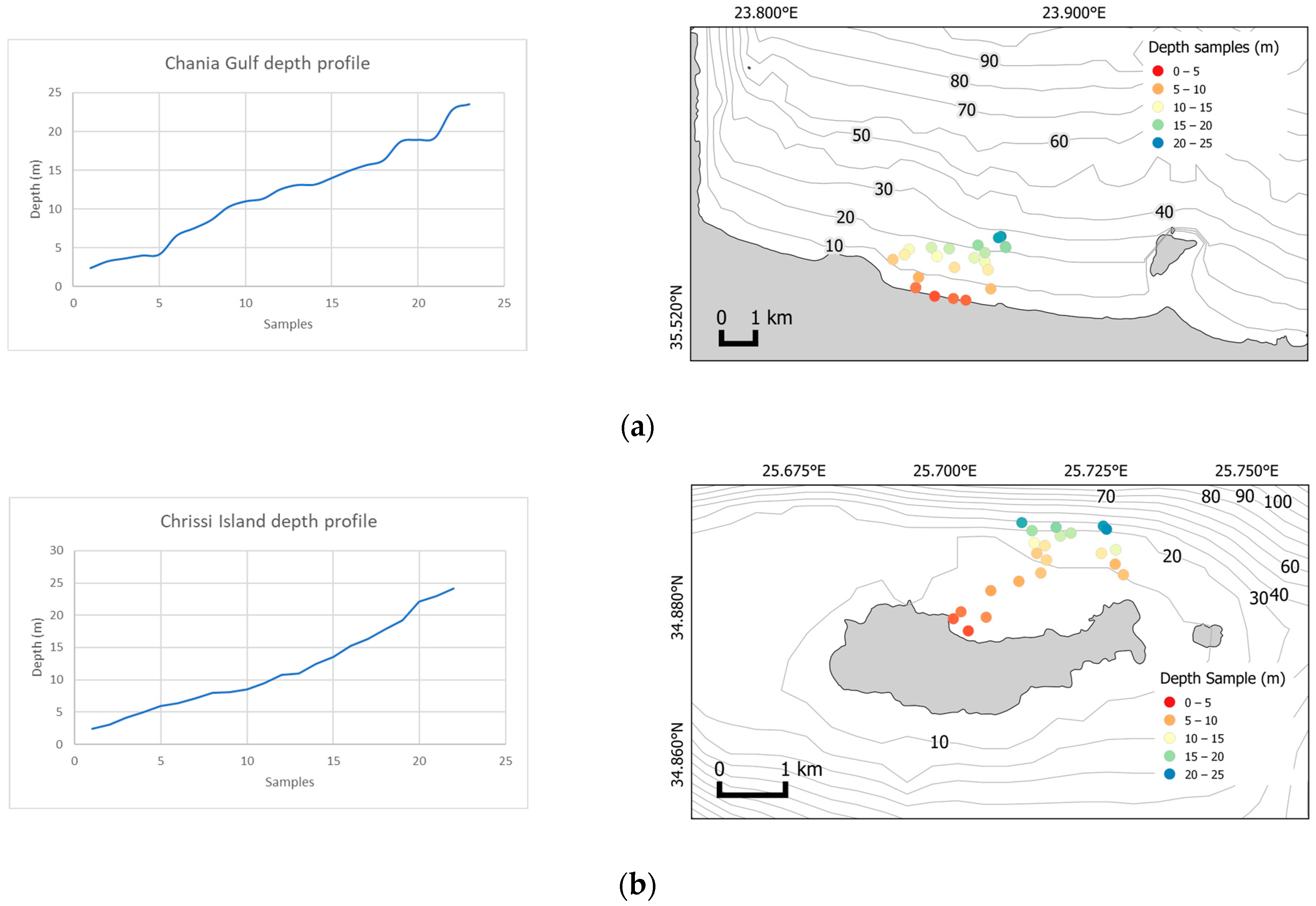
2.1. Study Area
2.2. Satellite Data
2.3. Field Data
3. Methods
3.1. Empirical Satellite-Derived Bathymetry (SDB)
3.2. Kalman Filter (KF) Smoothing
3.3. Water’s Optical Properties
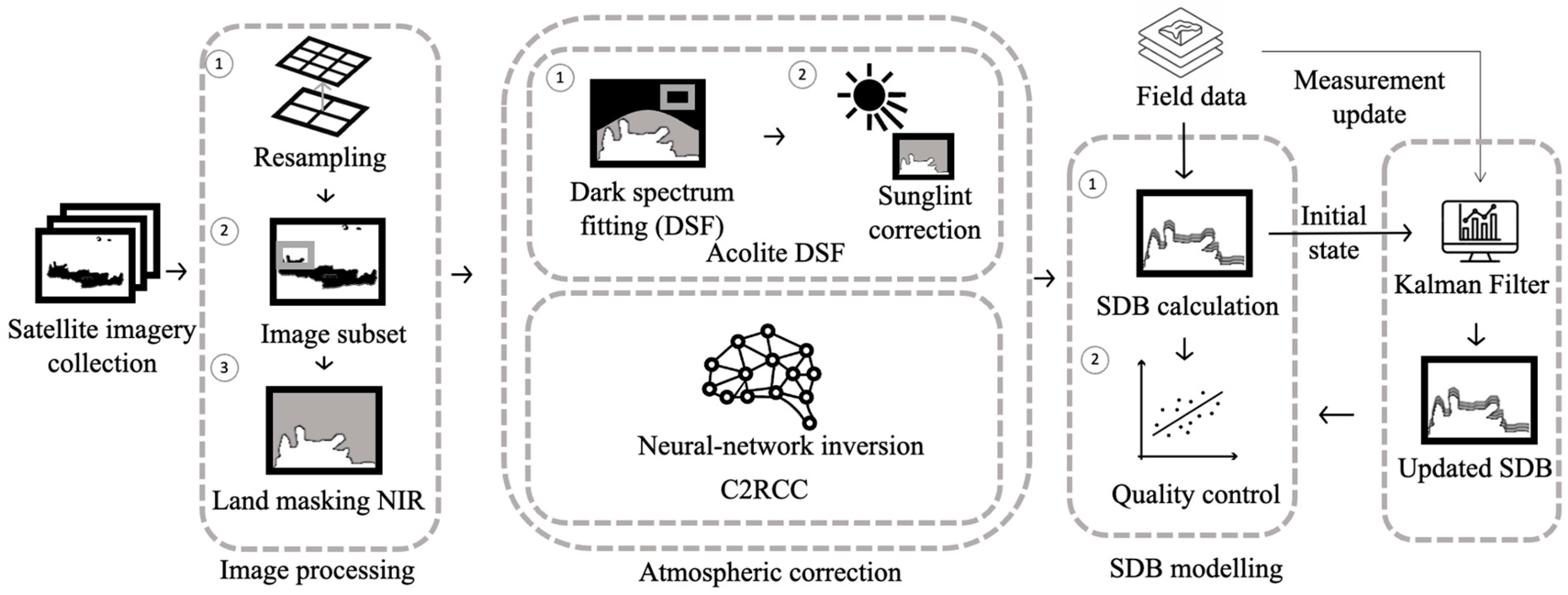
3.4. Workflow
4. Results
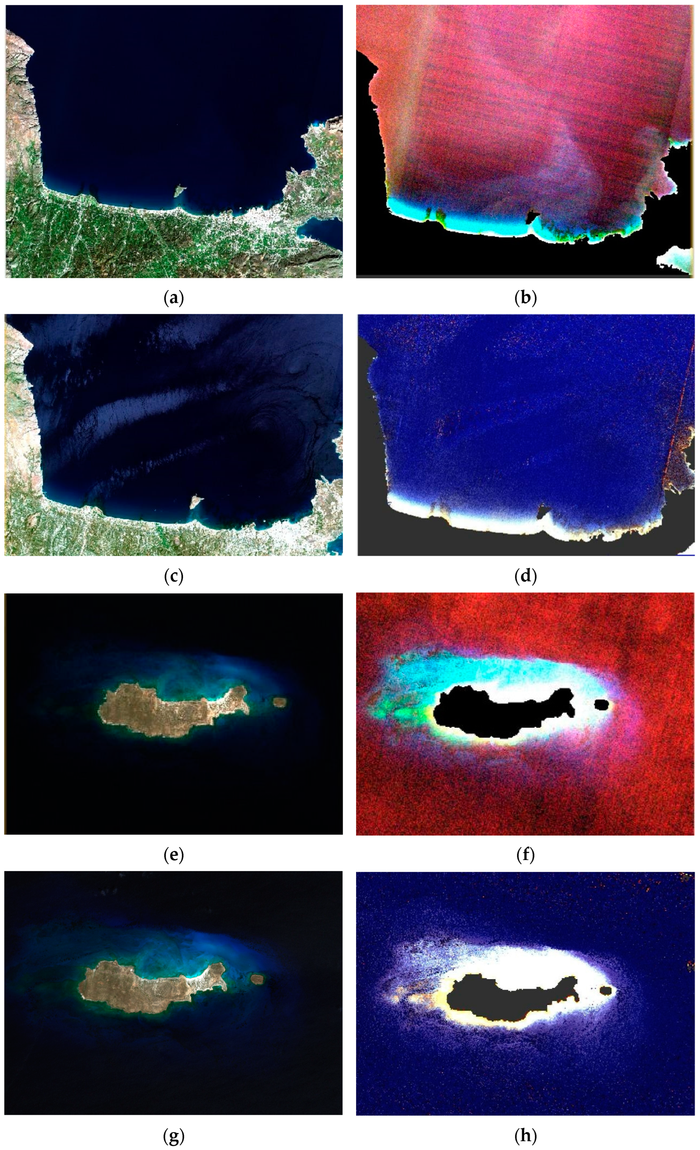
4.1. Atmospheric Correction
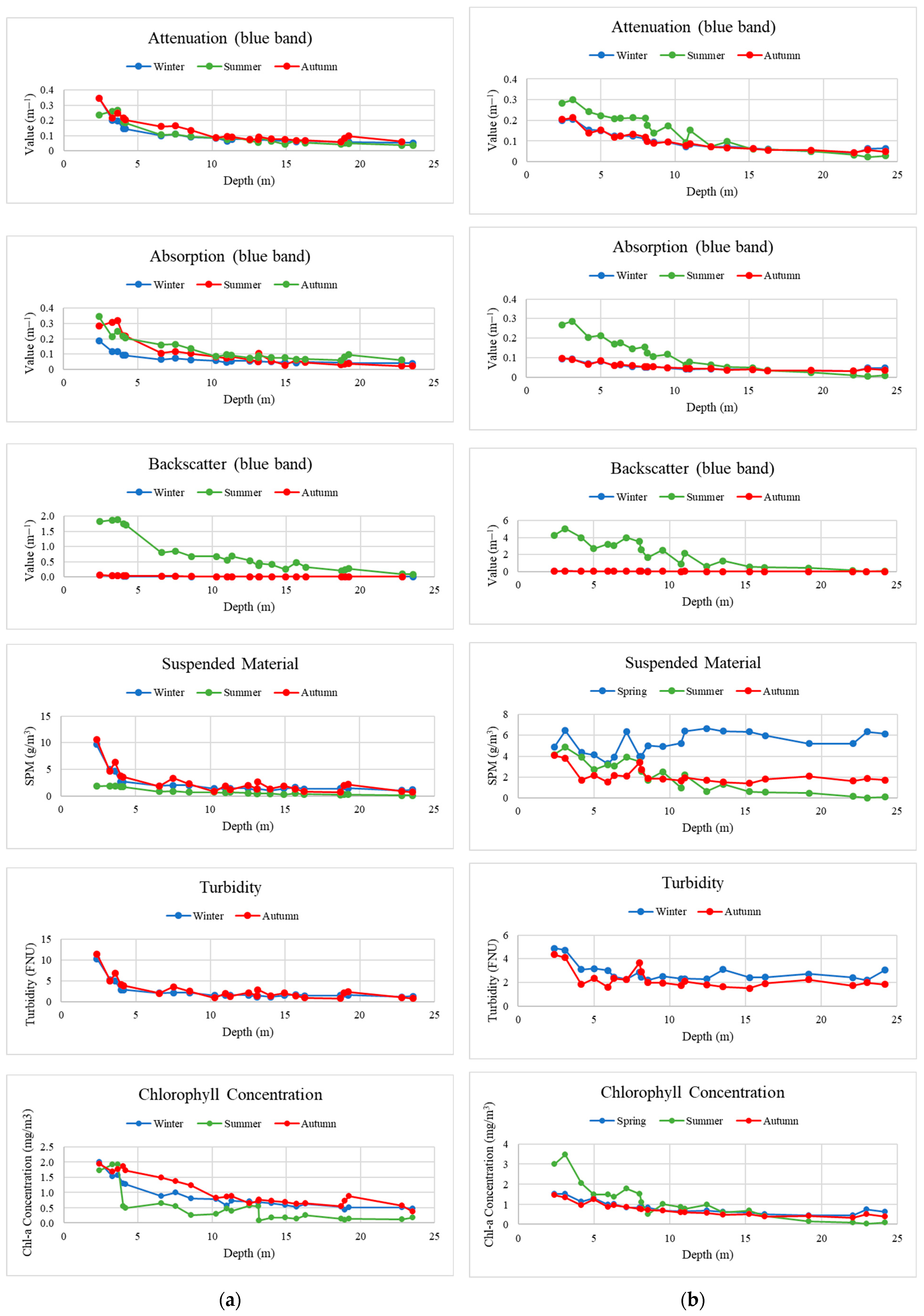
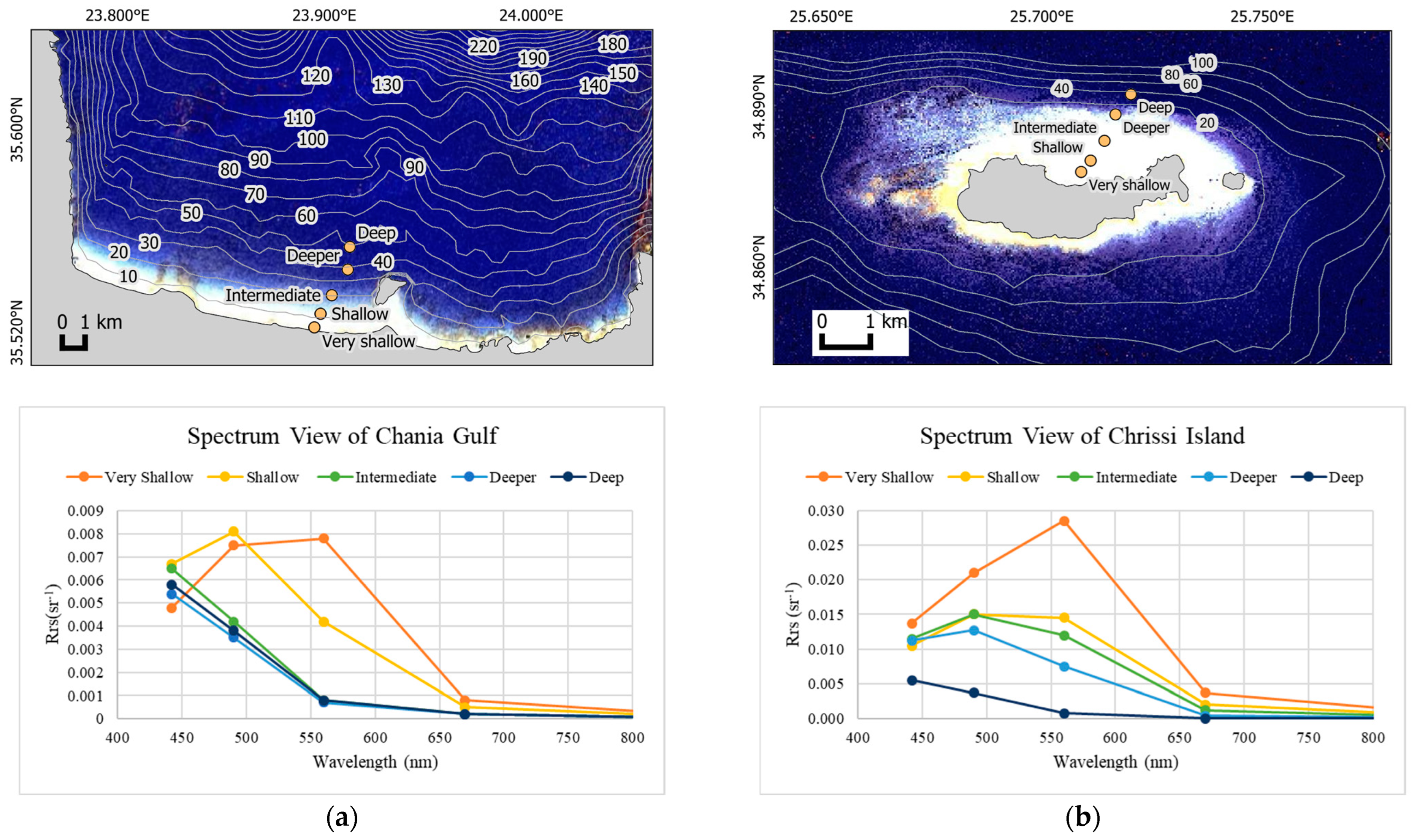
4.2. Optical Water Properties Analysis
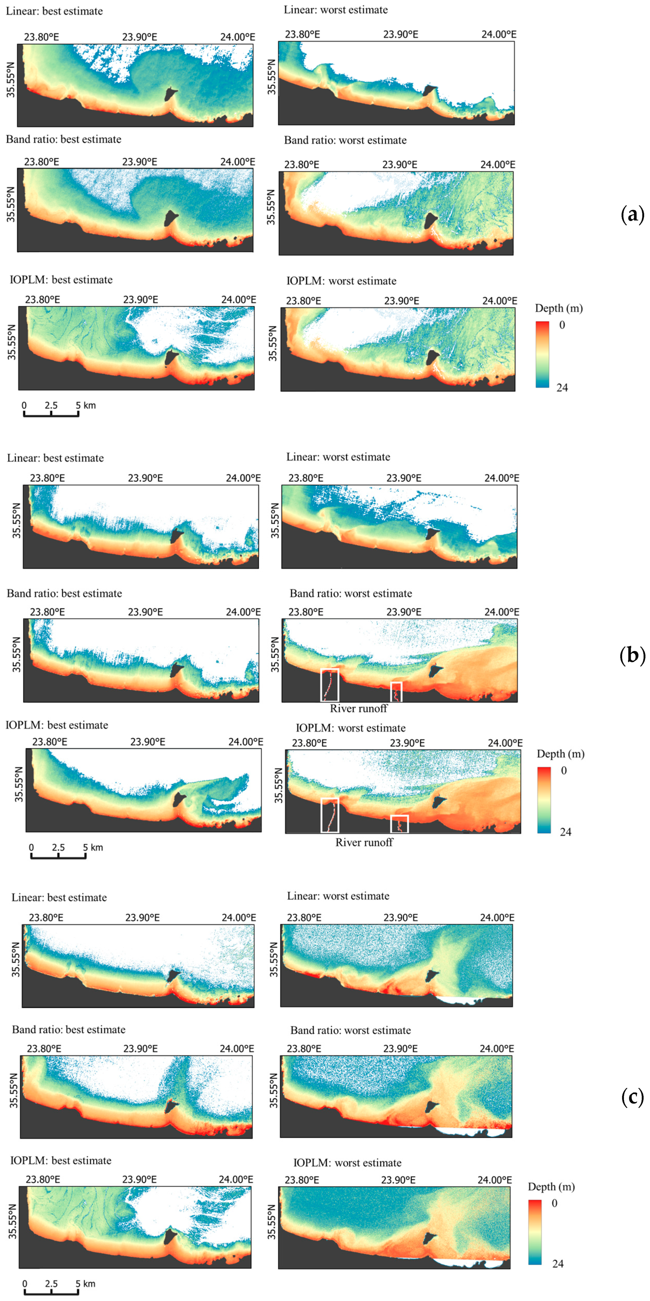
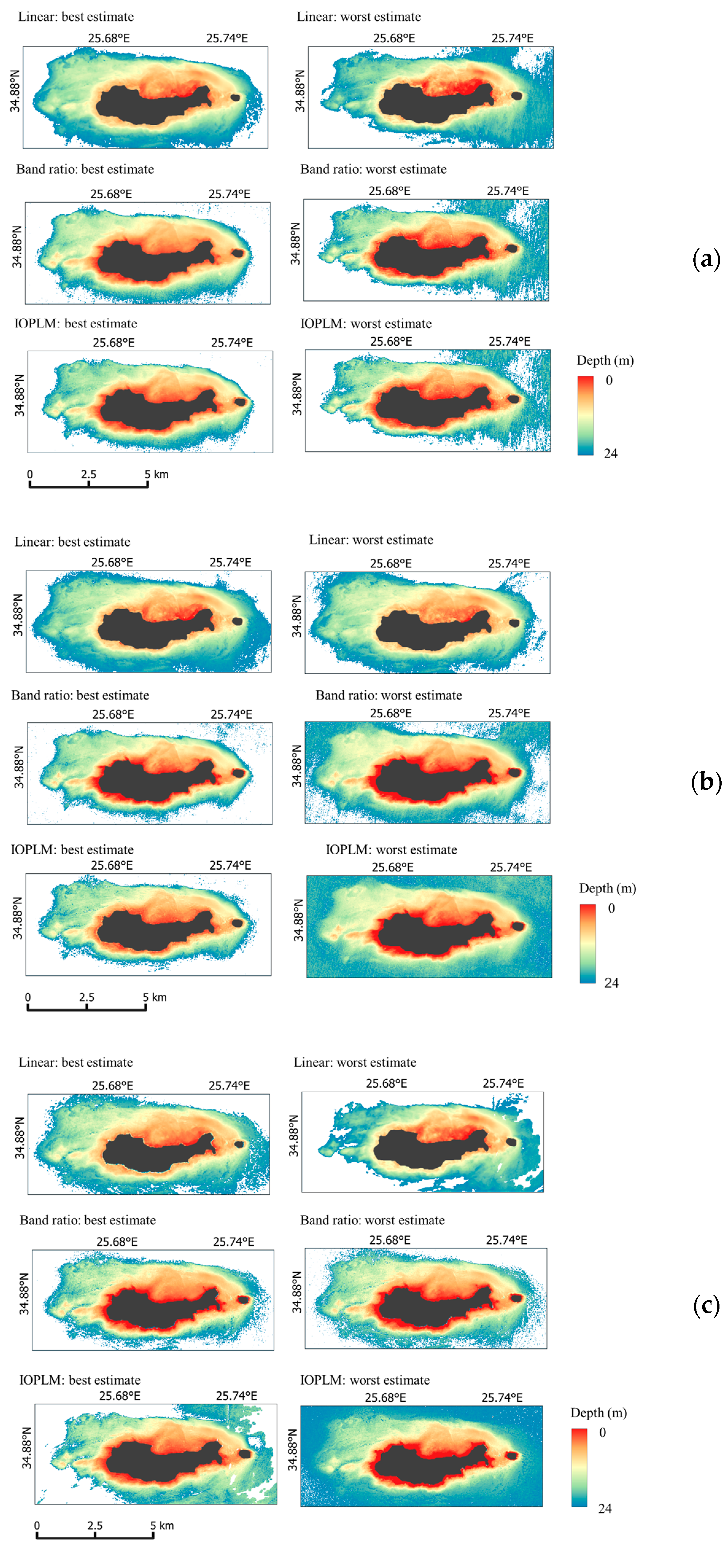
4.3. SDB Model
5. Discussions
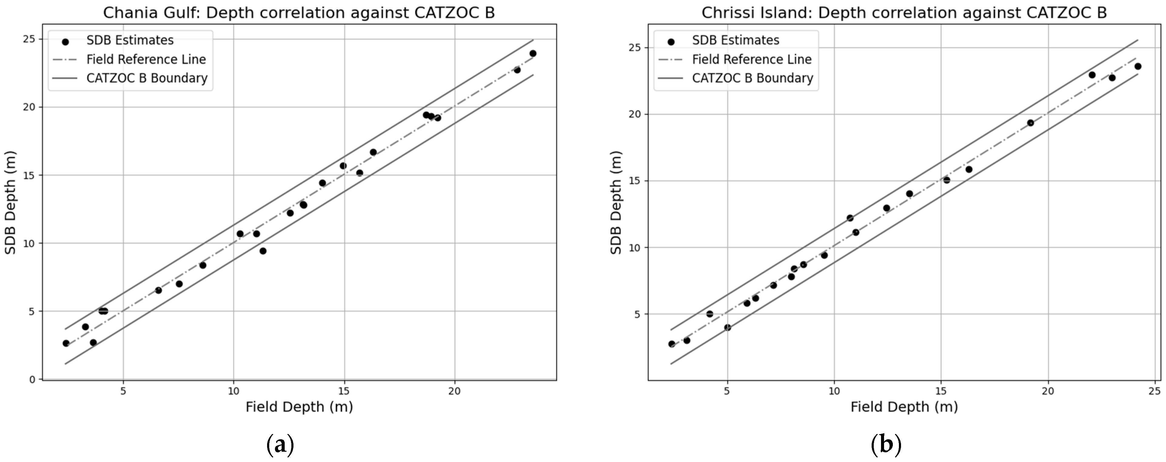
5.1. Assessment of Model Accuracy
5.2. Kalman Filter (KF)
6. Conclusions
7. Future Research
Author Contributions
Funding
Data Availability Statement
Acknowledgments
Conflicts of Interest
References
- Ashphaq, M.; Srivastava, P.K.; Mitra, D. Review of Near-Shore Satellite Derived Bathymetry: Classification and Account of Five Decades of Coastal Bathymetry Research. J. Ocean Eng. Sci. 2021, 6, 340–359. [Google Scholar] [CrossRef]
- Louvart, P.; Cook, H.; Smithers, C.; Laporte, J. A New Approach to Satellite-Derived Bathymetry: An Exercise in Seabed 2030 Coastal Surveys. Remote Sens. 2022, 14, 4484. [Google Scholar] [CrossRef]
- Stumpf, R.P.; Holderied, K.; Spring, S.; Sinclair, M. Determination of Water Depth with High-Resolution Satellite Imagery over Variable Bottom Types. Limnol. Oceanogr. 2003, 48, 547–556. [Google Scholar] [CrossRef]
- Lyzenga, D. Passive Remote-Sensing Techniques for Mapping Water Depth and Bottom Features. Appl. Opt. 1978, 17, 379–383. [Google Scholar] [CrossRef]
- Jupp, D. International Journal of Remote Reconstruction of Sand Wave Bathymetry Using Both Satellite Imagery and Multi-Beam Bathymetric Data: A Case Study of the Taiwan Banks. In Proceedings of the Symposium on Remote Sensing of the Coastal Zone, Gold Coast, QLD, Australia, 7–9 September 1988. [Google Scholar]
- Lee, Z.; Carder, K.L.; Arnone, R.A. Deriving Inherent Optical Properties from Water Color: A Multiband Quasi-Analytical Algorithm for Optically Deep Waters. Appl. Opt. 2002, 41, 5755. [Google Scholar] [CrossRef]
- Zhang, X.; Ma, Y.; Zhang, J. Shallow Water Bathymetry Based on Inherent Optical Properties Using High Spatial Resolution Multispectral Imagery. Remote Sens. 2020, 12, 3027. [Google Scholar] [CrossRef]
- Streftaris, N.; Zenetos, A.; Papathanassiou, E. Globalisation in Marine Ecosystems: The Story of Non-Indigenous Marine Species across European Seas. Oceanogr. Mar. Biol. 2005, 43, 419–453. [Google Scholar] [CrossRef]
- Mandlburger, G. A Review of Active and Passive Optical Methods in Hydrography. Int. Hydrogr. Rev. 2022, 28, 8–52. [Google Scholar] [CrossRef]
- Chaikalis, S.; Parinos, C.; Möbius, J.; Gogou, A.; Velaoras, D.; Hainbucher, D.; Sofianos, S.; Tanhua, T.; Cardin, V.; Proestakis, E.; et al. Optical Properties and Biochemical Indices of Marine Particles in the Open Mediterranean Sea: The R/V Maria S. Merian Cruise, March 2018. Front. Earth Sci. 2021, 9, 614703. [Google Scholar] [CrossRef]
- Drakopoulou, P.; Kapsimalis, V.; Parcharidis, I.; Pavlopoulos, K. Retrieval of Nearshore Bathymetry in the Gulf of Chania, NW Crete, Greece, from WorldWiew-2 Multispectral Imagery. Proc. SPIE 2018, 54, 10773. [Google Scholar] [CrossRef]
- Natura 2000 Natura 2000—Standard Data Form: Site GR4340003. Available online: https://natura2000.eea.europa.eu/Natura2000/SDF.aspx?site=GR4340003 (accessed on 3 September 2023).
- ESA S2 MSI ESL Team. Copernicus Space Component Sentinel Optical Imaging Mission Performance Cluster Service Sentinel-2 Annual Performance Report-Year 2022. 2023. Available online: https://sentinel.esa.int/documents/247904/4868341/OMPC.CS.DQR.001.12-2022+-+i83r0+-+MSI+L1C+DQR+January+2023.pdf (accessed on 28 July 2023).
- Mobley, C.D. The Oceanic Optics Book; IOCCG: Dartmouth, NS, Canada, 2022; 924p. [Google Scholar] [CrossRef]
- Lyzenga, D. Shallow-Water Bathymetry Using Combined Lidar and Passive Multispectral Scanner Data. Int. J. Remote Sens. 1985, 6, 115–125. [Google Scholar] [CrossRef]
- Chybicki, A. Mapping South Baltic Near-Shore Bathymetry Using Sentinel-2 Observations. Polish Marit. Res. 2017, 24, 15–25. [Google Scholar] [CrossRef]
- Kutser, T.; Hedley, J.; Giardino, C.; Roelfsema, C.; Brando, V.E. Remote Sensing of Shallow Waters—A 50 Year Retrospective and Future Directions. Remote Sens. Environ. 2020, 240, 111619. [Google Scholar] [CrossRef]
- Goodman, J.A.; Lee, Z.P.; Ustin, S.L. Influence of Atmospheric and Sea-Surface Corrections on Retrieval of Bottom Depth and Reflectance Using a Semi-Analytical Model: A Case Study in Kaneohe Bay, Hawaii. Appl. Opt. 2008, 47, F1–F11. [Google Scholar] [CrossRef] [PubMed]
- Lee, Z.; Hu, C.; Shang, S.; Du, K.; Lewis, M.; Arnone, R.; Brewin, R. Penetration of UV-Visible Solar Radiation in the Global Oceans: Insights from Ocean Color Remote Sensing. J. Geophys. Res. Ocean. 2013, 118, 4241–4255. [Google Scholar] [CrossRef]
- Philpot, W.D. Bathymetric Mapping with Passive Multispectral Imagery. Appl. Opt. 1989, 28, 1569. [Google Scholar] [CrossRef]
- IOCCG. Remote Sensing of Inherent Optical Properties: Fundamentals, Tests of Algorithms, and Applications; IOCGG: Dartmouth, NS, Canada, 2006; Volume 5, ISBN 9781896246567. [Google Scholar]
- Vanhellemont, Q. Adaptation of the Dark Spectrum Fitting Atmospheric Correction for Aquatic Applications of the Landsat and Sentinel-2 Archives. Remote Sens. Environ. 2019, 225, 175–192. [Google Scholar] [CrossRef]
- Vanhellemont, Q. Sensitivity Analysis of the Dark Spectrum Fitting Atmospheric Correction for Metre- and Decametre-Scale Satellite Imagery Using Autonomous Hyperspectral Radiometry. Opt. Express 2020, 28, 29948. [Google Scholar] [CrossRef]
- Caballero, I.; Stumpf, R.P. Atmospheric Correction for Satellite-Derived Bathymetry in the Caribbean Waters: From a Single Image to Multi-Temporal Approaches Using Sentinel-2A/B. Opt. Express 2020, 28, 11742. [Google Scholar] [CrossRef]
- Brockman, C.; Doerffer, R.; Peters, M.; Stelzer, K.; Embacher, S.; Ruescas, A. Evolution of the C2RCC Neural Network for Sentinel 2 and 3 for the Retrieval of Ocean Colour Products in Normal and Extreme Optically Complex Waters. Living Planet Symp. 2004, 740, 54. [Google Scholar]
- Ribeiro, M.I. Kalman and Extended Kalman Filters: Concept, Derivation and Properties; Institute for Systems and Robotics: Lisboa, Portugal, 2004; p. 42. [Google Scholar]
- Mobley, C.D.; Stramski, D.; Paul Bissett, W.; Boss, E. Optical Modeling of Ocean Waters: Is the Case 1–Case 2 Classification Still Useful? Oceanography 2004, 17, 60–67. [Google Scholar] [CrossRef]
- Mavraeidopoulos, A.K. Satellite Derived Bathymetry with No Use of Field Data. In Proceedings of the 2nd International Conference on Design and Management of Port, Coastal and Offshore Works, Thessaloniki, Greece, 24–27 May 2013; pp. 1–8. [Google Scholar]
- Mavraeidopoulos, A.K.; Oikonomou, E.; Palikaris, A.; Poulos, S. A Hybrid Bio-Optical Transformation for Satellite Bathymetry Modeling Using Sentinel-2 Imagery. Remote Sens. 2019, 11, 2746. [Google Scholar] [CrossRef]
- Chavez, P.S. An Improved Dark-Object Subtraction Technique for Atmospheric Scattering Correction of Multispectral Data. Remote Sens. Environ. 1988, 24, 459–479. [Google Scholar] [CrossRef]
- Traganos, D.; Poursanidis, D.; Aggarwal, B.; Chrysoulakis, N.; Reinartz, P. Estimating Satellite-Derived Bathymetry (SDB) with the Google Earth Engine and Sentinel-2. Remote Sens. 2018, 10, 859. [Google Scholar] [CrossRef]
- RBINS. ACOLITE User Manual (QV—2 August 2021); Royal Belgian Institute of Natural Sciences (RBINS): Brussels, Belgium, 2021. [Google Scholar]
- Hollingsworth, A.; Engelen, R.J.; Textor, C.; Benedetti, A.; Boucher, O.; Chevallier, F.; Dethof, A.; Elbern, H.; Eskes, H.; Flemming, J.; et al. Toward a Monitoring and Forecasting System for Atmospheric Composition: The GEMS Project. Bull. Am. Meteorol. Soc. 2008, 89, 1147–1164. [Google Scholar] [CrossRef]
- Doerffer, R.; Schiller, H. The MERIS Case 2 Water Algorithm. Int. J. Remote Sens. 2007, 28, 517–535. [Google Scholar] [CrossRef]
- Nechad, B.; Ruddick, K.G.; Neukermans, G. Calibration and Validation of a Generic Multisensor Algorithm for Mapping of Turbidity in Coastal Waters. In Remote Sensing of the Ocean, Sea Ice, and Large Water Regions; SPIE: Bellingham, WA, USA, 2009; Volume 7473. [Google Scholar] [CrossRef]
- Nechad, B.; Ruddick, K.G.; Park, Y. Calibration and Validation of a Generic Multisensor Algorithm for Mapping of Total Suspended Matter in Turbid Waters. Remote Sens. Environ. 2010, 114, 854–866. [Google Scholar] [CrossRef]
- Chai, T.; Draxler, R.R. Root Mean Square Error (RMSE) or Mean Absolute Error (MAE)? -Arguments against Avoiding RMSE in the Literature. Geosci. Model Dev. 2014, 7, 1247–1250. [Google Scholar] [CrossRef]
- Willmott, C.J.; Matsuura, K. Advantages of the Mean Absolute Error (MAE) over the Root Mean Square Error (RMSE) in Assessing Average Model Performance. Clim. Res. 2005, 30, 79–82. [Google Scholar] [CrossRef]
- Makridakis, S. Accuracy Measures: Theoretical and Practical Concerns. Int. J. Forecast. 1993, 9, 527–529. [Google Scholar] [CrossRef]
- IHO. S-44 6th Edition: IHO Standards For Hydrographic Surveys; IHO: Monaco-Ville, Monaco, 2020. [Google Scholar]
- Copernicus Marine Service (CMEMS). Sea Water Potential Temperature. Available online: https://marine.copernicus.eu/access-data (accessed on 27 August 2023).
- Yin, M.Q.; Wang, L.; Zhao, S.M. Experimental Demonstration of Influence of Underwater Turbulence on Ghost Imaging. Chin. Phys. B 2019, 28, 1–6. [Google Scholar] [CrossRef]
- Ghorbanidehno, H.; Lee, J.; Farthing, M.; Hesser, T.; Kitanidis, P.K.; Darve, E.F. Novel Data Assimilation Algorithm for Nearshore Bathymetry. J. Atmos. Ocean. Technol. 2019, 36, 699–715. [Google Scholar] [CrossRef]
- Herrmann, J.; Magruder, L.A.; Markel, J.; Parrish, C.E. Assessing the Ability to Quantify Bathymetric Change over Time Using Solely Satellite-Based Measurements. Remote Sens. 2022, 14, 1232. [Google Scholar] [CrossRef]
- Miller, R.L.; Del Castillo, C.E.; Mckee, B.A. Remote Sensing of Coastal Aquatic Environments; Springer: New York, NY, USA, 2005; ISBN 9781402030994. [Google Scholar]
- Mohamed, H.; Nadaoka, K.; Nakamura, T. Towards Benthic Habitat 3D Mapping Using Machine Learning Algorithms and Structures from Motion Photogrammetry. Remote Sens. 2020, 12, 127. [Google Scholar] [CrossRef]


| Year | Season | Sensing Date (UTC Time) | Sun Zenith Angle (Degree) | Sun Azimuth Angle (Degree) | View Zenith Angle (Degree) | View Azimuth Angle (Degree) | Glint (Degree) |
|---|---|---|---|---|---|---|---|
| Chania Gulf | |||||||
| Spring | 07-March-2019 | 44.59 | 152.74 | 3.05 | 215.23 | 43.25 | |
| 2019 | Summer | 09-August-2019 | 25.11 | 137.32 | 3.09 | 215.46 | 24.65 |
| Autumn | 28-October-2019 | 49.99 | 164.69 | 3.13 | 213.80 | 47.98 | |
| Winter | 31-January-2020 | 56.19 | 157.58 | 3.11 | 213.76 | 54.50 | |
| 2020 | Summer | 28-August-2020 | 30.05 | 146.45 | 3.16 | 216.21 | 29.09 |
| Autumn | 07-September-2020 | 33.02 | 150.82 | 3.16 | 216.19 | 31.82 | |
| Spring | 06-March-2021 | 44.77 | 152.84 | 3.16 | 216.12 | 43.42 | |
| 2021 | Summer | 24-June-2021 | 18.9 | 125.73 | 3.12 | 214.59 | 19.08 |
| Autumn | 07-October-2021 | 43.03 | 160.88 | 3.15 | 215.14 | 41.25 | |
| Winter | 19-February-2022 | 50.32 | 154.85 | 3.14 | 214.94 | 48.81 | |
| 2022 | Summer | 18-August-2022 | 27.26 | 141.65 | 3.18 | 216.57 | 26.59 |
| Autumn | 27-October-2022 | 49.76 | 164.60 | 3.14 | 214.76 | 47.79 | |
| Chrissi Island | |||||||
| Spring | 19-March-2019 | 39.50 | 149.45 | 3.56 | 122.09 | 36.37 | |
| 2019 | Summer | 21-August-2019 | 27.70 | 140.30 | 3.51 | 123.17 | 24.37 |
| Autumn | 25-October-2019 | 48.36 | 163.00 | 3.51 | 123.16 | 45.71 | |
| Winter | 23-January-2020 | 57.44 | 157.70 | 3.56 | 122.27 | 54.56 | |
| 2020 | Summer | 30-August-2020 | 30.28 | 145.03 | 3.51 | 123.42 | 27.04 |
| Autumn | 13-November-2020 | 54.27 | 164.79 | 3.47 | 123.74 | 51.69 | |
| Spring | 13-March-2021 | 41.63 | 150.29 | 3.50 | 123.10 | 38.54 | |
| 2021 | Summer | 30-August-2021 | 30.21 | 144.91 | 3.49 | 122.66 | 27.01 |
| Autumn | 24-October-2021 | 48.20 | 162.93 | 3.45 | 125.80 | 45.49 | |
| Winter | 11-February-2022 | 52.44 | 154.67 | 3.50 | 123.60 | 49.47 | |
| 2022 | Summer | 20-August-2022 | 27.53 | 139.93 | 3.57 | 122.69 | 24.14 |
| Autumn | 04-October-2022 | 41.31 | 158.50 | 3.50 | 123.49 | 28.49 | |
| SDB Method | Metric | Value (m) |
|---|---|---|
| Linear | RMSE | 1.81 |
| RMSE updated | 0.47 | |
| MAE | 1.48 | |
| MAE updated | 0.37 | |
| MedAE | 1.16 | |
| MedAE updated | 0.30 | |
| IOPLM | RMSE | 0.54 |
| RMSE updated | 0.05 | |
| MAE | 0.40 | |
| MAE updated | 0.04 | |
| MedAE | 0.27 | |
| MedAE updated | 0.02 |
Disclaimer/Publisher’s Note: The statements, opinions and data contained in all publications are solely those of the individual author(s) and contributor(s) and not of MDPI and/or the editor(s). MDPI and/or the editor(s) disclaim responsibility for any injury to people or property resulting from any ideas, methods, instructions or products referred to in the content. |
© 2025 by the authors. Licensee MDPI, Basel, Switzerland. This article is an open access article distributed under the terms and conditions of the Creative Commons Attribution (CC BY) license (https://creativecommons.org/licenses/by/4.0/).
Share and Cite
Muhammad, F.; Tsimpouxis, I.; Sternberg, H. Investigating the Impact of Spatiotemporal Variations in Water Surface Optical Properties on Satellite-Derived Bathymetry Estimates in the Eastern Mediterranean. Remote Sens. 2025, 17, 444. https://doi.org/10.3390/rs17030444
Muhammad F, Tsimpouxis I, Sternberg H. Investigating the Impact of Spatiotemporal Variations in Water Surface Optical Properties on Satellite-Derived Bathymetry Estimates in the Eastern Mediterranean. Remote Sensing. 2025; 17(3):444. https://doi.org/10.3390/rs17030444
Chicago/Turabian StyleMuhammad, Fickrie, Ioannis Tsimpouxis, and Harald Sternberg. 2025. "Investigating the Impact of Spatiotemporal Variations in Water Surface Optical Properties on Satellite-Derived Bathymetry Estimates in the Eastern Mediterranean" Remote Sensing 17, no. 3: 444. https://doi.org/10.3390/rs17030444
APA StyleMuhammad, F., Tsimpouxis, I., & Sternberg, H. (2025). Investigating the Impact of Spatiotemporal Variations in Water Surface Optical Properties on Satellite-Derived Bathymetry Estimates in the Eastern Mediterranean. Remote Sensing, 17(3), 444. https://doi.org/10.3390/rs17030444