Abstract
The exchange of water, sediment, and nutrients in wetlands occurs through a complex network of channels and overbank flow. Although optical sensors can map channels at high resolution, they fail to identify narrow intermittent channels colonized by vegetation. Here we demonstrate an innovative application of rapid-repeat interferometric synthetic aperture radar (InSAR) to study hydrologic connectivity and tidal influences in Louisiana’s coastal wetlands, which can provide valuable insights into water flow dynamics, particularly in vegetation-covered and narrow channels where traditional optical methods struggle. Data used were from the airborne UAVSAR L-band sensor acquired for the Delta-X mission. We applied interferometric techniques to rapid-repeat (~30 min) SAR imagery of the southern Atchafalaya basin acquired during two flights encompassing rising-to-high tides and ebbing-to-low tides. InSAR coherence is used to identify and differentiate permanent open water channels from intermittent channels in which flow occurs underneath the vegetation canopy. The channel networks at rising and ebbing tides show significant differences in the extent of flow, with vegetation-filled small channels more clearly identified at rising-to-high tide. The InSAR phase change is used to identify locations on channel banks where overbank flow occurs, which is a critical component for modeling wetland hydrodynamics. This is the first study to use rapid-repeat InSAR to monitor tidal impacts on water flow dynamics in wetlands. The results show that the InSAR method outperforms traditional optical remote sensing methods in monitoring water flow in vegetation-covered wetlands, providing high-resolution data to support hydrodynamic models and critical support for wetland protection and management.
1. Introduction
Coastal wetlands throughout the world are losing land due to rising sea levels and anthropogenic activities [1,2,3,4], and gaining vertical elevation through sediment accretion is one key to their survival [5]. Channel networks connect wetlands to the nearby water bodies and play a crucial role in exchanging water, sediment, and nutrients in wetlands [6]. Mapping the spatial distribution of the channels and depth of inundation provides proxy information on the propagation of hydrodynamic energy, vegetation type and growth, and sediment transport and deposition [7]. Water flow in coastal wetlands is dynamic at multiple spatial and temporal scales, varying with seasonal river discharge, ocean tides, and episodic events affecting any connected water bodies [8]. In coastal wetlands, tidal conditions regulate the availability of water on daily to seasonal scales. Wider “open/perennial channels” receive water during all seasons and actively conduct water into the wetlands, whereas some narrow “intermittent/non-perennial channels” receive water only during flood seasons and high tidal conditions and can become colonized with vegetation [9,10]. Exchange from the channels into the interiors of the wetlands occurs as the water from the channels overflows the banks (overbank flow) and through secondary channels that extend into the interior of the islands. Flow extent on the land depends on the resistance to the flow offered by the vegetation, infiltration locations, and channel water levels among many other factors [11]. As the flow velocity reduces on the wetland surface, sediment in the water settles out, contributing to wetland elevation gain that counters subsidence and sea-level rise [12,13,14]. The net contribution from land elevation change (positive or negative) and sea-level rise is called relative sea-level rise (RSLR).
Previous studies have shown that both the presence of channels and the absence of barriers to flow are necessary for wetland hydrologic connectivity [15]. Friction caused by vegetation, siltation within the channels, clogging of sand and vegetation, erosion along the margins, natural levees, and artificial structures like roads and ditches are some of the means by which water transport is obstructed, and the connectivity disruption can lead to wetland degradation [16]. In areas with natural or artificial levees, overbank flow from the channel onto the land occurs only if the water level can overcome the levee height, which is generally higher than the land in the island interior. Field observations have revealed that small channels that run deep into the interior of the wetland islands also play an important role in transporting large quantities of water to the interior [17]. Small, mounded sediment deposits that form at the mouths of these small channels ultimately cause uneven distribution of sediments and nutrients over the island [18]. Thus, identifying locations of overbank flow and small, possibly intermittent, channels in the wetlands can improve understanding of hydrodynamic connectivity.
Studies monitoring the vulnerability of wetlands use hydrodynamic models, which require detailed information on the spatial distribution of channels, locations receiving overbank flow, and the flow distribution on the land to determine which parts of the wetland are likely to gain land in the future [19]. In the absence of models, observational information on which islands are receiving overbank flow can also be an indicator of the health of the wetlands, showing which areas could be nourished with sediment [20,21,22]. In many small channels filled with vegetation, water flow occurs mainly beneath the plant cover. Most channel network maps fail to identify these intermittent and vegetated channels, although knowing their location is critical for accurate hydrodynamic models that simulate the flow conditions in wetlands [23,24]. In general, hydrodynamic models utilize flow paths derived from channel centerlines and require a better representation of all the possible flow paths to simulate the flow conditions at different discharge levels [25,26]. So far, wide-scale mapping of locations receiving overbank flow, choke points in the channel connectivity, and leakage through levee breaks has not been performed using remote sensing.
Most wetland classification studies do not explicitly focus on resolving water channels but generically classify water bodies, making them less resolvable from roads and other linear features [27]. Precisely resolving the boundaries of the channels adjacent to the wetlands and the variation in their extent during different seasons and tidal conditions is valuable information to improve hydrodynamic models. A major challenge here is that the width and extent of the mapped channels depend on prevailing discharge conditions during mapping. Most channel maps are intended to show the channel network under conditions in which the channel is full, ignoring overbank flow, in order for the width of the channel to be sufficiently well represented in models [28]. But in highly dynamic areas like coastal wetlands subject to both seasonal variations in river discharge and daily tidal exchange, flow conditions are not uniform across the image or static in time, making mapping the channels difficult.
Optical sensors are most commonly used to map the channels [29] but are limited by their spatial resolution and by occlusion from clouds and plants. Unlike optical imagery, synthetic aperture radar (SAR) can image through clouds, without the need for solar illumination, and in some cases image the surface below vegetation. SAR also has the capability to differentiate some features that may not be visually separable, e.g., channels and roads [30]. Each SAR single-look complex (SLC) image contains intensity and phase information, which are related to the surface properties, scattering mechanism, and distance to the surface. Interferometry uses two SLCs to obtain the change in phase between the two acquisitions, which is related to the cumulative surface displacement, including water-level change in parts of wetlands where there is double-bounce scattering between the water surface and emergent vegetation [31,32].
Identifying localized flow on the channel banks with satellite-based SAR instruments is challenging due to their often low spatial resolution, low signal-to-noise ratio for wetland surfaces, particularly water, and loss of interferometric coherence over the days-to-weeks between repeat imaging, which can seriously degrade measurements in vegetated areas. SAR intensity images alone have been used previously to identify flooded or inundated areas in many parts of the world, particularly those areas subject to sheet flow (e.g., [33,34]). However, such methods require a long timeseries of images [35] or fusion with optical data [36] to identify small channels that are covered with vegetation. Previous studies with InSAR have largely focused on detecting tidal or seasonal variation in water level over large areas in the wetland interiors (sheet flow measurements) [37,38,39,40], not on identifying the water-level change over the channel banks, a mechanism by which water reaches the interiors in the absence of the high water levels of sheet flow across the landscape [38,41].
In this study, we show the capabilities of rapid-repeat InSAR from an airborne platform for mapping permanent and intermittent channels as well as overbank flow adjacent to the channels in the wetlands of the Wax Lake Delta and Atchafalaya basin in coastal Louisiana. In this area, the riparian wetlands are well connected to water sources by a network of channels that dissect the landscape into small interdistributary islands surrounded by water [17,42]. The measurements collected with the Uninhabited Aerial Vehicle SAR (UAVSAR) comprise a unique dataset in which measurements are repeated at sub-hourly intervals (~30 min) and with relatively high spatial resolution facilitating the study of the tidal exchange of water from channels to the wetland island interiors. Data were collected in two ~2.5 h flights on consecutive days, one when the tide was rising towards high tide and the other in which the tide was ebbing near low tide. This study specifically looks at flow within the channels and from the channels to the islands at a local scale, not at sheet flow across the landscape, because of the relatively short interval over which each data set was collected. Given the observed distributary network and progression of flow within the wetlands, we examine the water flow in and around the islands to investigate how water moves between the channels and the wetlands and how that differs across a tidal cycle. By integrating rapid-repeat InSAR phase and coherence analysis, this study fills the gap in monitoring intermittent flow paths that traditional optical sensors fail to detect. This is also the first use of both the InSAR phase and coherence timeseries to map channel networks and water flow within coastal wetlands using data covering different stages of the tidal cycle.
2. Study Area
The study focuses on the lower Mississippi Delta region of coastal Louisiana, USA. The delta has been a hotspot of land loss due to erosion and RSLR. Land subsidence due to geologic and anthropogenic processes exacerbates the effect of the RSLR [43,44,45,46,47,48,49,50]. Studies have shown that coastal Louisiana is losing wetlands at a rate of up to 90 km2/year [51,52]. However, the pattern of loss is not uniform, and there are some areas observed to be gaining land [53]. The specific study site is the Wax Lake Delta and the lower Atchafalaya basin (Figure 1a), a region that has been gaining land ever since the Wax Lake Outlet was dug in 1941 to reduce floods in Morgan City, Louisiana, by diverting the discharge from the Atchafalaya River. This diversion results in the Wax Lake Delta area receiving ~34 million tons of sediment per year [54].
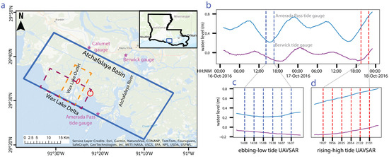
Figure 1.
(a) Study area showing the UAVSAR image footprint (blue rectangle) and other areas discussed in the text. (b) Water level at the Amerada Pass and Berwick tide gauges during the two days of the UAVSAR acquisitions. (c,d) Plots showing the tidal variation during the ebbing-to-low tide (c) and rising-to-high tide (d) UAVSAR flights. The times of the UAVSAR acquisitions are indicated with vertical lines.
Figure 1a shows the study area, the site of freshwater wetlands with diverse vegetation and soil types that receive water from the Wax Lake Outlet and the Atchafalaya River, plus from the Gulf of Mexico through tides. Though the area receives a mean annual discharge of 2000–3000 m3/s through the Wax Lake Outlet (measured at Calumet gauge, Figure 1), oceanic tidal conditions exert major control over the water-level variation in areas close to the coast [17]. The primary channels dissecting the wetlands are >100 m wide, and numerous secondary channels carry water from the primary channels to the interior of the wetlands. Some of these secondary channels are intermittent and are only active during times of high discharge. Water levels in the area can vary >1 m between the dry and wet seasons [40]. Spring months (February–June) experience flood conditions in the area with more discharge from the Wax Lake Outlet [55] compared to fall months (August–November).
3. Data
3.1. SAR Data (UAVSAR)
Rapid-repeat InSAR data were acquired by the UAVSAR L-band SAR on two consecutive flight days in autumn 2016 and covered different parts of the tidal cycle [56]. The flights were part of the NASA Delta-X Earth Venture-Suborbital mission [22], which collected airborne data over parts of the lower Mississippi River Delta in multiple campaigns covering low and high river discharge and different stages of the tidal cycle, including pre-Delta-X campaigns in 2015 and 2016. The Delta-X mission studies the hydrodynamics of the delta with multiple remote sensing instruments, field measurements, and models simulating the terrain and flow conditions. The UAVSAR swath width is ~22 km and the incidence angle varies ~22–67° from the near to far range of the swath [56]. The aircraft is operated along a controlled flight track within a 10 m diameter tube centered on the planned track [57]. Final images are delivered as co-registered SLC stacks after correcting for aircraft motion and topography. The spatial resolution of the SLC product is 0.8 m in the along-track (azimuth) direction and 1.7 m in the across-track line-of-sight (slant range) direction.
The UAVSAR image footprint is shown in Figure 1a. The imaged area covers the parts of the Atchafalaya basin where significant land gain has been observed in the past century [53] and the extent was chosen to image the wetlands between the Wax Lake Outlet and the Atchafalaya River to support Delta-X hydrodynamic models [22]. We used HH-polarization (horizontal transmit, horizontal receive) imagery for the analysis as it is more sensitive to double-bounce scattering, which is key for deriving water-level change measurements [58]. The SAR data were specifically acquired to track the water movement in the delta at varying tidal conditions. Data were collected during both ebbing-to-low tide (16 October 2016) and rising-to-high tide (17 October 2016) during flights of duration ~2.5 h (6 acquisitions for each tide condition). Figure 1b shows the water level during the two days, measured at the NOAA Amerada Pass and Berwick tide gauges. The tidal heights are referenced to the local tidal datum of mean lower low water height. Repeat imagery was acquired at ~30 min intervals to capture the turning of the tide and limit water-level change between acquisitions to ~5 cm or less (Figure 1b). The repeat interval is also limited by the time the aircraft took to image the area and then return to repeat it.
The Amerada Pass tide gauge is located in the near range of the SAR image and shows the water level as the tide enters the study area (https://tidesandcurrents.noaa.gov/stationhome.html?id=8764227#available (accessed on 17 January 2024)). The Berwick tide gauge is located beyond the far range of the SAR image, so the difference between the gauges indicates the spatial variation in tidal conditions across the image. Close to the mouth of the estuary, tides are highly influenced by oceanic conditions; hence, the Amerada Pass tide gauge shows larger tidal amplitude than the Berwick gauge because of water spreading inland through channels branching off the main channel. Away from the coast, the flow velocity is more influenced by channel depth and bed friction. The time lag in the tidal level between the two locations is approximately 2 h during rising tide and 3 h during ebbing tide (computed as lag between the peaks and troughs of the two tidal levels as plotted in Figure 1b). Figure 1c,d shows the water level at the two NOAA gauges during each of the two flights, and vertical lines indicate the UAVSAR acquisition times. The corresponding UAVSAR product names are given in Supplement S1.1. In the description of the data and results corresponding to the tidal conditions, we refer to the rising-high tide period as “rising tide” and the ebbing-low tide period as “ebbing tide”.
The UAVSAR data are openly available for download from the data portal (https://uavsar.jpl.nasa.gov/ (accessed on 15 April 2024)) or Oak Ridge National Laboratory Distributed Active Archive Center (DAAC) (https://daac.ornl.gov/ (accessed on 15 April 2024) [56]). We perform interferometric processing as described in Section 4 to derive coherence measurements and timeseries of water-level change.
3.2. Optical Data
To validate and compare UAVSAR-derived channel masks, we used two water masks derived using two different Normalized Difference Water Index () implementations based on data from the National Agriculture Imagery Program (NAIP) and the Airborne Visible/Infrared Imaging Spectrometer-Next Generation (AVIRIS-NG; https://avirisng.jpl.nasa.gov/ (accessed on 1 May 2024)). Both NAIP and AVIRIS-NG operate in the visible to near-infrared spectrum with AVIRIS-NG operating further into the shortwave-infrared (SWIR) wavelengths. Channel masks derived from them are referred to as optical masks for comparison with the SAR-derived channel mask. NAIP imagery is given in 4 bands (Red, Blue, Green, and Near Infrared (NIR)) and AVIRIS-NG has data in 425 bands with a spectral resolution of 5 nm in the ~375 to 2500 nm wavelength range. is calculated as follows:
is the observed intensity in each spectral band, with the green and NIR bands used for the NAIP imagery (1). An threshold of ≥0.1 was used to classify pixels as water in NAIP imagery [59]. A different using SWIR band was implemented to generate water masks from the Delta-X AVIRIS-NG data (Equation (2) of [60]). The green and SWIR bands at ~562.4 and ~1609.2 nm, respectively, were used to calculate , which has proven effective in similar implementations at minimizing the confusion between water with aquatic vegetation present and land [61]. An NDWI2 threshold of ≥0.1 was used to classify pixels as water in the AVIRIS-NG data.
AVIRIS-NG data were collected during the Delta-X campaign over the study area in September 2021 (imaged date is 24 September 2021). The NAIP water mask was derived using from five years (2010, 2013, 2015, 2017, and 2019) of airborne data using Google Earth Engine [62]. NAIP imagery was acquired at different times in a year, and temporal composites were created for each year by calculating the mean of all the images in the corresponding year (acquisition dates in Supplement S1.3). Pixels identified as water in at least two of the five years were marked as water. Because the data were acquired over multiple seasons, the NAIP mask has more channels compared to the AVIRIS-NG mask. The AVIRIS-NG data nearly match the resolution of UAVSAR masks at 4.8 m, but the NAIP mask was initially derived at 1 m resolution and then resampled to 5 m to match the resolution of the UAVSAR masks for comparison.
4. Methodology
The preliminary processing to obtain InSAR phase change, coherence, and water-level change is described in detail in [58] and is summarized here. Each SLC pixel has amplitude and phase information stored as a complex number. The difference in phase between the two SLCs can be related to water-level change in the wetlands after compensating for other contributions [58]. SAR interferometry is sensitive to changes in the surface between acquisitions, and the similarity between two images is quantified by a property called coherence () [63], defined as follows:
where and are the complex representations of two different SLCs. E indicates the expected value computed in a multilooking window. In this analysis, the SLCs were multilooked to suppress noise (12 looks in azimuth, 3 looks in range), bringing the resolution to ~5 m × 7 m.
We observed that the change in coherence with time varies between different types of surfaces, and we used this to differentiate land from water flow paths. To calculate the phase and coherence changes between the acquisitions, for each flight date, we formed interferograms between each SLC and the next three acquired SLCs. Doing this yielded three sets of interferograms for each tidal condition: one set with all interferograms having temporal baselines of 30 min, one with all interferograms having temporal baselines of 60 min, and the third for interferograms with temporal baselines of 90 min. These are referred to as the nearest neighbor (NN), NN+1, and NN+2 interferograms for 30, 60, and 90 min baselines, respectively. This choice ensured that coherence was maintained in the network for phase unwrapping and also provided tighter constraints on timeseries inversion, the process by which the phase changes in multiple temporally overlapping interferograms are converted measurements of water-level change vs. time [58,64]. We used standard processing tools available through the ISCE 2.0 package [65] for interferogram generation and the MintPy (v1.5.0) package [66] for timeseries analysis.
The prevalence of water channels that dissect land into islands makes unwrapping interferograms difficult. We followed the guidelines outlined in [58] and implemented the standard error correction processes (phase bridging and phase closure) iteratively to improve the unwrapping. In phase bridging, regions that are locally well unwrapped yet spatially isolated from the other regions are connected to avoid phase jumps between the regions [66]. The phase closure algorithm checks and corrects for phase inconsistencies in time-overlapped interferograms [64]. Unwrapped phase measurements () in radians were converted to cm for better understanding and representation (see Supplement S1.2). The unwrapped interferograms were inverted using MintPy to derive phase timeseries (cm) referenced to the first acquisition. This relates directly to the cumulative water-level change evaluated at the acquisition times. Using a linear fit to the phase timeseries, InSAR phase velocity () in cm/h was computed to compare the water-level change rates at different locations within the SAR scene. Both and provide a spatial snapshot of water-level changes over the land area as the exchange of water takes place between channels and islands. Higher phase changes are observed in areas nearer to the coast and along major canals (e.g., Wax Lake Outlet). values on pixels bordering the channels were used to identify locations of overbank flow onto land beyond the channel edges.
Below, we describe the use of InSAR coherence over different time intervals to classify the image pixels into land (wetland) or water (channels) categories (Section 4.1). We calculated the loss of interferometric coherence between SAR acquisitions and observed that coherence loss in interferograms of temporal separation > 30 min is extremely sensitive to narrow channels where flow occurs under the vegetation. We then used image morphological operations to extract pixels that lie adjacent to the water channels (Section 4.2), which were combined with InSAR phase measurements (from phase timeseries or phase velocity) to map locations of bank overflow where water flows from the channels into the wetlands (Section 4.3).
4.1. Water Channel Network from SAR Coherence
Open water surfaces generally lose coherence rapidly [67] because of small-scale wave motion on the surface resulting from wind roughening and currents. Given the rapid-repeat interferograms, we observed that open water surfaces like the main water channels have coherence < 0.4 even in the 30 min interferograms, whereas the other areas maintained coherence in the 30 min interferograms to varying degrees depending upon the surface characteristics. With this threshold, we identified most of the wider channels, but identifying small, narrow channels that extend into the middle of the wetlands required further analysis.
Narrow channels containing vegetation can have high coherence due to double bounce scattering between the water and emergent vegetation. In this case, the coherence varies as the water level changes, depending on the amount of emergent vegetation (Figure 2e). Such channels exhibit low coherence, equivalent to the large open channels, when the water level is high enough to inundate the vegetation completely (Figure 2e). To demonstrate the coherence variation in time, we used a high-resolution (1 m) aerial image acquired in September 2017 (close in time to our UAVSAR data) to identify some representative locations for open water, wetland, and narrow vegetation-filled channels in an island close to the coast (Supplement S4). The mean coherence over these three classes at increasing time intervals is plotted in Figure 2f and clearly shows that the narrow channel pixels have high coherence in the 30 min interferograms, but their coherence decreases rapidly after that. Hence, using the coherence for intervals greater than 30 min is critical to identify such small channels. In our study area, interferograms with intervals greater than 90 min have shown a rapid decline in coherence, rendering them not useful for interferometric processing. From the stacks of interferograms for rising tide and ebbing tide, considered separately, we computed the mean coherence of interferograms with uniform temporal separation, obtaining three maps giving the mean coherence of each set of interferograms (NN, NN+1, and NN+2) for each flight. We then averaged the coherence for the NN+1 and NN+2 stacks for a given flight to get NN1 and 2. This yields two average coherence maps for each tidal condition, namely, the mean coherence for a temporal interval of 30 min (NN) and another for intervals > 30 min (NN1 and 2), which are shown in Figure 2 for rising tide and ebbing tide. Figure 2b,d show that the mean coherence of NN1 and 2 interferograms () can identify more channels within the wetlands than the channels identified in Figure 2a,c using the mean coherence of NN interferograms (). These additional channels are mostly narrow secondary channels and channels contributing to intermittent flow in the wetlands and are mainly visible in our rising-tide dataset when the water level in the wetlands is significantly higher (Figure 1b). For this reason, the rising-tide data are used to generate water masks with three classes: open water channels, small/intermittent channels, and wetlands, where this latter class encompasses land that is not inundated plus those vegetated wetland areas where the water-level change was too small to measurably impact the InSAR coherence or phase.
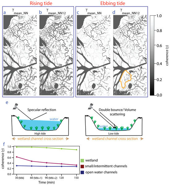
Figure 2.
Mean coherence image of NN and NN1 and 2 interferograms for the Wax Lake Delta area during rising tide (a,b) and ebbing tide (c,d) (Geographic location and extent of the area are shown with a purple dotted rectangle in Figure 1. See Supplement Figure S1 for full frame version). (e) Illustration showing the water level in a channel containing vegetation and SAR backscatter from the channel surface depending on the presence of emergent vegetation, which varies across the tidal cycle. (f) Variation in coherence with time over pixels identified as open water, wetland, and small/intermittent channels (locations were identified using high-resolution NAIP imagery (Supplement Figure S4)). Orange line in (d) shows the island used to identify representative locations for (f).
We classify channels using the rising-tide NN coherence as open water channels and the rising-tide NN1 and 2 coherence as small/intermittent channels. To derive a channel mask that differentiates between open water and intermittent channels, we first calculated the histogram of (Figure 3a—averaged over the 5 interferograms) and (Figure 3b—averaged over the 7 interferograms). We then chose a threshold on each histogram to identify the difference between land and water. We used a threshold of < 0.4 to identify open water channels and ≥ 0.4 and < 0.5 to identify intermittent channels (Figure 3c). These thresholds were manually chosen to account for the mixed pixels along the channel edges and should be adjusted for other datasets (e.g., different sensors, temporal spacing, spatial resolution, and multilook factors). While using additional thresholds on phase or amplitude or implementing supervised classification methods may perform better in correctly identifying the extent of the channels, in this study, we aim to show the predictive capability of a single variable, namely, the interferometric coherence, that can be applied to other study areas. In Section 6.4, we address the challenges of incorporating the InSAR phase for channel delineation, and in Section 6.5, we discuss the limitations of the method in general and potential future directions.
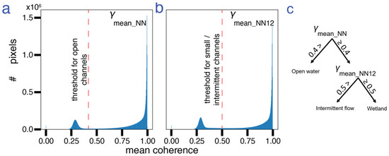
Figure 3.
Histograms of mean coherence of (a) NN and (b) NN1 and 2 rising-tide interferograms. (c) Flowchart of the steps to derive the channel maps from coherence showing the thresholds used. Pixels below the threshold are identified as open water channels. Pixels below the threshold are identified as intermittent channels only if they are not identified as open water pixels.
4.2. Image Morphology to Derive Channel Bank Masks
Once the coherence-based channel mask was generated delineating the small and intermittent channels, the mask was converted to a binary mask of land and water pixels (i.e., water pixels include both open water channels and intermittent channels). We then grew connected components (CCs) on the binary mask to separate land areas between the channels into small islands [68]. The CC generation consists of a common region-growing algorithm where an input image with the foreground (land) and background (water) pixels is separated into regions of contiguous pixels with an assigned label for each foreground region. The algorithm groups all contiguous land pixels with at least one land pixel in eight of its neighboring pixels into a unique region (i.e., one CC) and assigns an integer label to it. An example of the CCs generated from a binary mask for a region over the Wax Lake Delta is shown in Figure 4a. For operational convenience, we removed CCs smaller than 5000 pixels (0.125 km2). To extract pixels on the banks of the channel, we performed a morphological erosion operation, which removes a specified number of pixels along the boundary of each CC. In our case, we eroded 10 pixels, i.e., 50 m in width around each CC (Figure 4b). A subtraction operation between the original and eroded CCs leaves the “channel bank” pixels (Figure 4c), which are used as a channel bank mask. The thresholds for minimum size of CCs and width of erosion were chosen visually for the study area based on the phase velocity measurements (Figure 5c), which indicate the spatial extent of water-level change around the channels. These should be adjusted for other datasets.
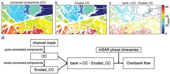
Figure 4.
(a) Connected components grown over channel mask. (b) Connected components after morphological erosion operation. (c) Channel bank pixels obtained after subtracting (b) from (a). (d) Flowchart of the steps to derive overbank flow from channel mask and phase timeseries. Geographic location and extent of the area in are shown with an orange dotted rectangle in Figure 1.
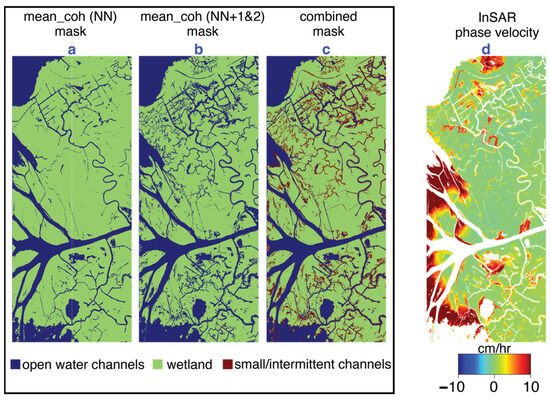
Figure 5.
(a) Channel mask using mean coherence of rising-tide NN interferograms; (b) channel mask using mean coherence of rising-tide NN1 and 2 interferograms; (c) combined mask retaining channels from (a) as open water channels and channels only in (b) as intermittent channels. The wetland category (green) contains pixels that maintained high average coherence in both NN and NN1 and 2 interferograms. (d) InSAR phase velocity from rising-tide data showing areas of water-level change. The warmer colors (yellow-red) indicate a rise in water level and the cooler colors (cyan-blue) indicate a fall in water level.
4.3. Mapping Overbank Flow
Changes in water level on the wetland surface are recorded as phase changes in SAR measurements. The phase observed near the channel banks changes as the water moves from the channel onto an island during rising tide and progressively decreases toward the interior of the island as the water spreads out into the island [69]. To isolate where the water level was changing on the channel banks, we applied the channel bank mask (Section 4.2, Figure 4c) to the phase timeseries and the phase velocity map. The steps involved in deriving phase measurements on channel banks are detailed in Figure 4d. Significant phase changes due to water-level changes on the channel bank are an indicator of overbank flow. In this way, we can identify locations at which the banks are lower and where the water is more likely to enter/exit the island.
In practice, locating overflow entails separating the water-level change signal on the channel banks from noise. In the rapid-repeat InSAR, the predominant source of phase noise is uncorrected atmospheric delay. The phase measurements can be contaminated by noise from the delay caused by differences in the atmosphere between the two acquisitions used to form an interferogram. For an airborne instrument, these are limited to changes in the troposphere, mainly from changes in air pressure, temperature, and water content (the “wet” troposphere) along the path through which the radar pulses propagate. In spaceborne SAR, there can be additional noise due to spatiotemporal variations in total electron content in the ionosphere [70,71]. Studies have observed that the turbulent delays caused by the variation in water vapor in the clouds are highly irregular in space and cannot be captured by weather models [72,73,74]. This occurs in our dataset also (see Section 5.3). In the InSAR community, the noise is commonly referred to as tropospheric delay (e.g., [75]) and can affect even rapid-repeat images. Traditional correction algorithms [76] rely on having weather data acquired at the same time as the SAR acquisitions, which can be difficult to obtain or not available at the needed spatial or temporal resolution of rapid-repeat InSAR [74,77,78]. Atmospheric phase delay can be of similar magnitude to the signal of interest (water-level change). Comparison with ground-based weather radars indicates that even small clouds cause phase delays of similar magnitude to the water-level change phase in L-band UAVSAR data acquired over the study area [72,73].
To address this issue and avoid using noise-contaminated data, we propose an approach to separate overbank flow using the relationship between phase change and water-level change during a tidal cycle. During rising tide as the water overflows the banks, the water level decreases from the channel banks towards the interior, so the phase change should be higher on the channel banks than in the interiors. To eliminate noisy data from consideration, for each CC, we compared the mean phase of the bank pixels to that of pixels in the island interior and retained only the CCs that have a higher mean positive phase on the banks than in the interiors, eliminating the others as being too low quality to assess bank overflow. This is the procedure for the rising-tide dataset; for ebbing tide, we considered CCs with higher mean negative phases on the banks than in the interiors since water would be moving from the island back into the channel. We note that this procedure does not work when there is sheet flow inundating an entire island during the interval covered by the InSAR dataset, but that is not the case for the dataset we used in this study, which was collected in October during low river discharge conditions.
5. Results
5.1. Water Channel Masks
Following the method described in Section 4.1, the mean coherences of the rising-tide dataset were used to derive three-state channel masks < 0.4 for open water channels and ≥ 0.4 and < 0.5 for small/intermittent channels). Figure 5a shows the open water channels derived from , Figure 5b shows small/intermittent channels derived from , and Figure 5c is the combined water mask. In the intermittent channels further inland, the increase in the flow depth during rising tide results in lower coherence in the >30 min interval interferograms. The combined mask significantly extends the channels that are mapped, particularly within the islands and further from the main channels.
The InSAR phase velocity at rising tide is also shown in Figure 5d. There are a few things to note regarding similarities and differences between the coherence and phase change maps in Figure 5. Firstly, the phase change is able to identify some of the intermittent channels, indicating their role in transporting water into the island interiors of the wetlands. In fact, Figure 5d shows that the InSAR phase information could potentially be used to derive locations of some narrow intermittent channels that are not identified using coherence alone. The phase also shows some challenges associated with the coherence method. In the Wax Lake Delta islands with a direct connection to the gulf waters (at the end of the Wax Lake Outlet, left side of image), the presence of dense, tall emergent vegetation resulted in high coherence from double-bounce scattering in all the acquisitions over the ~2.5 h period, hence yielding a higher average coherence than our threshold, which was selected based primarily on the values within the inland coastal wetlands. This is particularly evident in open-ended islands along the delta front, where the SAR phase velocity corresponds to water-level changes of ~10 cm/h, hence obviously had inundated vegetation, but the land is not identified as open water or intermittent channels based on the coherence thresholds. It is possible that a longer imaging interval would resolve this or different thresholds for islands bordering the gulf vs. those further inland. In this study, we elected not to use the phase information to form the combined mask (Figure 5c) due to the challenges and limitations of incorporating the InSAR phase that are discussed in Section 6.4.
5.2. Cross-Validation of the Water Channel Mask
Here we compare the SAR-derived channel mask to optical masks from AVIRIS-NG and NAIP. For the SAR coherence mask, we combined small/intermittent and open water channels into one “water” category for comparison. Figure 6 shows the three different masks and the comparison between them for the Wax Lake Delta and nearby inland wetlands. We denote the “wetland” category in the SAR mask as “land” for consistency. Table 1 shows the standard error matrix for channel classification using SAR coherence compared to optical imagery computed over the entire image frame of 7009 × 3300 pixels. For both comparisons, “land” is more accurately identified than “water”, and the agreement with the AVIRIS-NG “water” pixels is better than with the NAIP mask. In Figure 6d,e, we show the distributions of classification errors between the optical and SAR masks. False positive pixels (FP = land in optical, water in SAR) are shown in blue, and false negative pixels (FN = water in optical, land in SAR) are shown in red. Most of the FPs are due to the inability of the optical masks to identify narrow channels and the fact that the SAR-based classification identifies inundation along the channel edges as water. False negatives are mainly in the Wax Lake Delta islands open to the gulf, where some of the shallow water regions are classified as open water in the AVIRIS-NG and NAIP masks. The UAVSAR data were acquired in October, which is at the end of the growing season so these areas might be heavily vegetated, contributing significant double bounce scattering. Such areas retain high coherence if the water level is not high enough to significantly submerge the vegetation and hence are identified as land in the SAR mask. The fact that the AVIRIS-NG data were acquired in the same season (fall) as the UAVSAR data could account for the better agreement on open water outside the Wax Lake Delta. Since the NAIP data were acquired over multiple seasons, including spring when the river discharge levels are higher, it includes some of the water-logged areas in the interior of the wetland (see Section 6.1). Also, the 10-year span of the NAIP data includes potential channel and shoreline migration in the area. Even though the NAIP mask at 1 m resolution (see Supplement S3) shows some additional intermittent channels of narrower width; overall, the UAVSAR mask identifies more channels in the study area because it images water-level change in vegetation-filled channels.
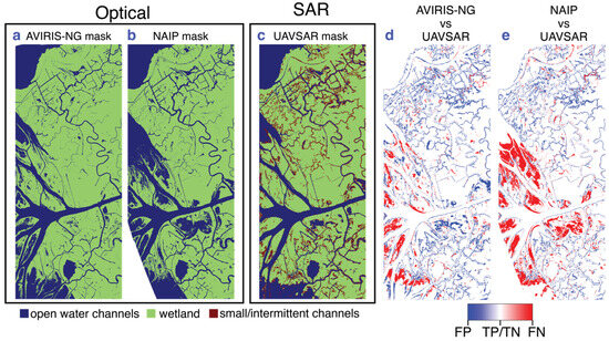
Figure 6.
Comparison of optical (a) AVIRIS-NG and (b) NAIP water channel masks with (c) UAVSAR mask. Classification accuracy indicating the location of water class FPs and FNs in the UAVSAR mask compared to (d) AVIRIS-NG and (e) NAIP masks. In d and e, white color indicates pixels’ class matches between both optical and SAR masks (see Supplement Figure S2 for full frame version).

Table 1.
Standard error matrix comparing channels identified with UAVSAR vs. NAIP and AVIRIS-NG optical imagery.
5.3. Overbank Flow: Separating Atmospheric Phase Delay from Water-Level Phase
We determined that the InSAR phase change can be very useful for identifying overbank flow. Three different areas are highlighted in Figure 7 to show the capability and limitations. To identify locations experiencing overbank flow, we start with the phase velocity () (Figure 7a), isolate pixels along the channel banks, and then identify and eliminate areas possibly affected by atmospheric noise before identifying locations of overbank flow (Figure 7b). Area 1 of Figure 7 is an example where the spatial extent of the atmospheric phase delay is smaller than the area of the CC, and here, the method correctly identifies noisy areas to be removed (area 1—Figure 7c–e). However, in some cases, if the influence of delay is uniformly distributed over the CCs (overbank flow is small and comparable to the noise), the method cannot identify the area as being noisy (area 2—Figure 7c–e). Also, if there is a small intermittent channel carrying flow into the interior of the wetland island, but the channel is not identified in the channel mask, it may be misidentified as noise (area 3—Figure 7c–e). The role of such small intermittent channels is discussed in Section 6.3. In summary, care needs to be taken to identify which CCs are removed due to potential noise contamination. We do not suggest this as a method to correct InSAR tropospheric noise but as a quality assurance method or guideline to avoid falsely identifying noise as water-level change in coastal wetlands, where wet troposphere is common. We note that this method cannot be used for wide-area sheet flow measurements in which phase change can uniformly vary across multiple CCs due to high volume water input that floods much of the land [32].

Figure 7.
(a) InSAR phase velocity () for the rising-tide data set containing signals from both water-level change and tropospheric water vapor delay, the latter particularly evident in the far range (right-hand side); (b) illustrated procedure to identify noisy CCs shown for a single CC; (c–e) procedure applied to three different areas indicated with black rectangles in (a): (c) InSAR phase velocity; (d) phase velocity averaged over the interior of each CC; (e) noisy CCs removed after comparison of average CC phase velocity to the average phase velocity on the CC’s bank. Dotted ellipses focus on the CCs illustrated.
6. Discussion
In this section, we discuss the features identified in the channel masks, how they can be used to study water transport within wetlands, and the potential of alternate SAR parameters such as interferometric phase to improve channel masks. We also examine the tidal dependence of the water channel extent and overbank flow. We finish by discussing the limitations of the method, challenges to applying it in other areas, and future work to address the remaining gaps.
6.1. Tidal Variations in Channel Flow
SAR systems with longer wavelengths (e.g., L-band) can better penetrate the vegetation canopy to map the flooding [79], thereby revealing more information about the paths along which water flows into island interiors. This is apparent in Figure 8, which shows the channel mask derived from the rising-tide dataset (Figure 8a) compared to what would be obtained if the ebbing-tide data were used (Figure 8b). SAR coherence is sensitive to the flow of water onto the banks during the rising-to-high tide, and comparison between the rising- and ebbing-tide channel masks shows that intermittent flow paths in the rising-tide channel mask (marked in red) better represent the channel widths. The channel network in the rising-tide data reveals, extends, and/or widens many small/intermittent channels, especially, but not only near the coast (compare Figure 8c,d). The distinction between the open water and intermittent channels is useful for understanding the hydrodynamic processes responsible for delivering sediments into wetlands. These intermittent channels indicate low-elevation land that might not be well represented in DEMs but contribute significantly to the transport and distribution of water and sediments within islands. Comparison of the ebbing- and rising-tide masks along the coast also show inundated areas with emergent vegetation at low tide that are totally submerged at high or near-high tide. The combination of high- and low-tide channel maps can be used to identify areas that have healthy flushing regimes and those that are cut off from the network.
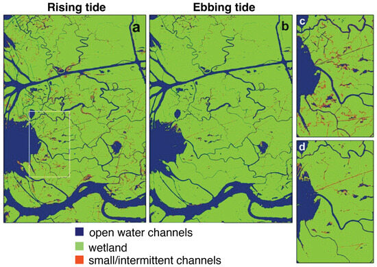
Figure 8.
(a) SAR channel mask derived from rising-tide InSAR data. (b) Equivalent channel network observed with SAR using the ebbing-tide InSAR data. (c) Focus on the rectangle in (a) for the rising-tide channel network and (d) ebbing-tide channel network.
Figure 9 compares the SAR-derived rising tide and optical channel masks. The SAR-derived channel mask (Figure 9a,b) consistently shows more intermittent channels in the interior of the wetlands than the optical masks (Figure 9c,d). Although optical instruments can identify open water surfaces, they cannot detect flow under the vegetation because they mainly image the top of the canopy [80]. Both optical masks are very similar to the ebbing-tide SAR mask (Figure 8b), indicating that the flow in channels only apparent in the rising-tide dataset is occurring for the most part below vegetation. Overall, the channel network determined with SAR better shows the hydrological connectivity than the optical-derived networks.
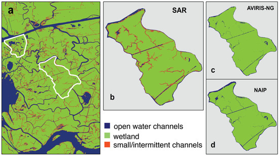
Figure 9.
(a) SAR channel mask and locations of islands (white polygons) showing the extent of intermittent channels identified by (b) SAR, (c) AVIRIS-NG, and (d) NAIP-derived channel masks. White polygon in (a) show the location of islands zoomed in (b–d).
6.2. Tidal Variation in Overbank Flow
Tidal flow variations influence daily water-level change dynamics in the wetland channels of our study area during the fall when river discharge is low [69]. As the tide propagates from the coast to the inland, there is a decrease in the tidal amplitude and a shift in the tidal phase as observed from the two gauges in Figure 1b. The water-level fluctuations are higher in areas closer to the delta front, in the channels close to the coast, and in the wider primary channels that are directly connected to the coast. Analogously, the islands adjacent to them have a greater chance of inundation as water overflows the banks, and islands further from the coast and the major channels should experience less overbank flow. This is observed in the UAVSAR data.
For the individual wetland islands, phase measurements on the banks can indicate the locations where the water is entering or exiting the islands, as discussed in Section 4.3. We have examined the phase changes on the channel banks as a function of time at rising and ebbing tides to determine how overbank flow progresses during the tidal cycle (Figure 10). In Figure 10, the timeseries shows progressively increasing phases on channel banks during rising tide (Figure 10a—warm colors), with the overflow occurring first in the islands of the Wax Lake Delta, directly connected to the gulf, then along the Wax Lake Outlet and channels closer to the coast, progressing further inland over time. Similar locations experienced progressively decreasing phases during ebbing tide (Figure 10b—cool colors). Identifying these locations provides information on when and where water is moving through the wetlands, which areas are receiving water and sediment from the channels, and how such dynamics vary over time. Using this information, hydrodynamic models can be calibrated for flow patterns and tuned to determine how different factors influence the flow of water in the wetlands (e.g., [23,81,82,83]). These models are important for predicting spatial patterns of sediment accumulation, e.g., in designing diversions to reclaim wetlands.

Figure 10.
Water-level increase and decrease identified by InSAR phase change on the banks of water channels as a function of time during (a) rising tide and (b) ebbing tide. Geographic location and extent of the area are shown with an orange dotted rectangle in Figure 1.
6.3. Exchange of Water from the Channel Network into the Wetland Interior
The channel mask (Figure 8) and the overbank flow sites (Figure 10) show the combination of processes exchanging water between the channels and the island interiors. A specific case using the InSAR phase change is shown in Figure 11. During rising tide, positive phase change is observed on some of the channel banks (Figure 11a), indicating water flow from the channels onto the edges of the islands, whereas during ebbing tide (Figure 11b), no negative phase is observed on the same banks, probably because the water level on the island was lower than the levee height preventing flow back into the channel at this location (see Figure 1). However, in both cases, the higher phase change is observed around a small channel extending into the island’s interior, indicating its role in transporting water during both high and low tides. Identifying where such transport is or is not occurring is important for wetland protection and restoration efforts because land loss from subsidence (as opposed to erosion) primarily occurs in the island interiors [84,85].
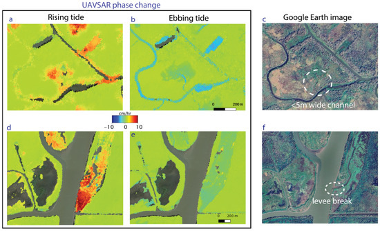
Figure 11.
UAVSAR phase change observed in the interior of the wetland during (a,d) rising tide and (b,e) ebbing tide. The difference between where the water goes during the different stages of the tides is clear. Overbank flow is more extensive at rising/high tide, but small channels still transport water within the island interior at ebbing/low tide. (c,f) Optical images to show the landscape (source: Google Earth [86,87]). Service Layer Credits: © 2024 Airbus. Geographic location of the areas in a&d are shown with red circle and ellipse in Figure 1.
In addition, repeated overbank flow can cause the levees to fail, which can bring more water onto the adjacent land and reduce the flow velocity in the channels [17]. Along the major channels carrying water into wetlands, levee failure can divert the supply from the channel, leading to the accumulation of water in certain locations. Such areas in the interior of the wetlands can be identified with InSAR as localized groups of pixels with high phase change adjacent to the channel (e.g., Figure 11d,e).
Field studies in the Wax Lake Delta have shown that connectivity between the channels and the interdistributary islands is mainly controlled by the secondary/intermittent channels and levees [17]. The presence of secondary channels and subaqueous levees was observed to facilitate water exchange, whereas subaerial levees and vegetated secondary channels impede the exchange. Spatial information on the location of narrow intermittent channels transporting water and areas where flow overtops the subaerial levees can be efficiently derived from SAR. Subaqueous levees cannot be identified with InSAR.
6.4. Use of InSAR Phase to Identify Small Channels
In addition to coherence, we also explored the capability of other SAR observables such as amplitude and interferometric phase to identify small channels. The UAVSAR instrument’s incidence angle varies too much over the swath width for amplitude to be used because the backscatter amplitude is a strong function of incidence angle. Thus, we focused on evaluating the use of the InSAR phase.
Within the wetlands, the presence of phase changes due to water-level changes around the channels can help to delineate the channels better in some areas, particularly for the small and intermittent channels. However, as discussed earlier, phase measurement in wetlands may be hindered by wet troposphere noise, making it hard to distinguish the small-scale phase changes from minor water-level changes. Figure 12 shows the InSAR phase velocity and a channel mask based on using thresholds on phase velocity (>2 cm/h for rising tide; <2 cm/h for ebbing tide) to extract channel extent. Adding phase-derived channels to coherence-derived channels can better delineate the channel network in some areas. However, phase noise due to the wet troposphere (e.g., right side warm colors in Figure 7a), although relatively low level, can obscure the channel network when the threshold is set to capture channels in areas without atmospheric noise. It is likely that machine learning algorithms could be trained to use the combination of phase and coherence to better delineate channel networks. Weather radar may also help eliminate areas where the InSAR phase is significantly impacted by wet troposphere delay [73].
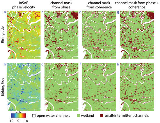
Figure 12.
(a,b) UAVSAR phase velocity showing water-level change rate for rising tide and ebbing tide; (c,d) channels derived using a threshold on phase; (e,f) channels derived using a threshold on coherence; and (g,h) channels derived using both phase and coherence.
6.5. Limitations and Future Directions
There are notable limitations to what can be carried out with InSAR and requirements for implementing the method elsewhere. First and foremost, the repeat interval has to be sufficiently short to track the tidal changes, and the acquisition interval has to be long enough to establish a timeseries of changes during a single tidal cycle. We used acquisitions over a 2.5 h period, which was long enough given 30 min repeats, and required both 60 min and 90 min repeats to best identify intermittent channels; 2.5 h or longer acquisition intervals and sub-hourly repeats are recommended for areas with similar tidal regimes to coastal Louisiana.
In addition, UAVSAR is a relatively high spatial resolution instrument (~5 m multilooked), and here, the UAVSAR mask identifies relatively few wetland channels that are less than 10 m. Past studies have shown the limitations of SAR systems in accurately identifying smaller water bodies [88,89], particularly ones smaller than twice the resolution of the sensor [33].
Furthermore, the measured SAR signal is a combination of the return from all elements on the ground within an imaged pixel. In some instances, e.g., where tall trees are along small channels, the return can be dominated by volume scattering from the trees or the return from the channel may be lost due to the layover phenomenon on steep-banked channels. Some of the channels close to the ocean are subaqueous and cannot be identified directly because the radar pulses cannot penetrate the water. However, the SAR amplitude has been used to identify large subaqueous channels on the Wax Lake delta front based on observation of a change in the water surface roughness due to faster currents and deeper water in the channels [90].
Moreover, the UAVSAR results presented here are influenced by the time of acquisition, which was in the fall. Whether more channels could be detected with SAR in the spring remains to be determined. It is possible that with high river discharge during spring, water flows through more remote channels, so more of the network is mapped. However, it is also possible that large areas are completely flooded, in which case the channels might not be apparent, or the tidal water input might not be sufficient to change the water level enough to be detected in rapid-repeat acquisitions.
Mapping the water-level changes under the vegetation can also depend on the SAR waves penetrating the canopy, which is a function of both canopy height and SAR wavelength [91]. Hence, if the vegetation canopy is thick and the wavelength of SAR is short (e.g., X-band, 3.3 cm), the return of the SAR wave is from the top of the canopy or from volume scattering in the top layers of the canopy and cannot map the water-level changes underneath the vegetation [92,93]. This phenomenon can affect the mapping of channels in swamps with tall trees [94].
For wetlands at high latitudes, icy conditions can lead to coherence on land even less than 0.4, thus reducing the ability to differentiate between channels and wetlands [95]. In some areas, wetlands are water-logged near-continuously (muddy and less vegetation—Figure 13d), and these areas might be identified as either land or water depending on the time of acquisition. The NAIP mask which is generated using acquisitions from multiple years taken during different seasons (both fall and spring) identified this area as water (Figure 13c), whereas the UAVSAR (Figure 13a) and AVIRIS-NG (Figure 13b) masks identified parts of the same area as water or land, probably because of differences in the time of acquisition, river stage, and vegetation cover. Also, the presence of the SWIR band in AVIRIS-NG could have resulted in a better classification of muddy areas compared to NAIP.
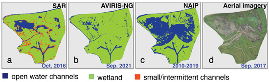
Figure 13.
The influence of acquisition time demonstrated on a continuously water-logged area in the interior of the wetland using close-ups of (a) SAR; (b) AVIRIS-NG; (c) NAIP-derived channel masks and (d) the aerial image of the corresponding area [96]. Geographic location and extent of the area are shown with a white polygon in Figure 9.
The thresholds chosen in our study for identifying water channels are based on the distribution of coherence among different land classes and the variation in coherence over time. While the method can be broadly applied to SAR data in other wetlands, care needs to be taken in choosing the thresholds. As in Figure 3, the dual peak nature of the coherence histogram clearly shows the coherence threshold of 0.4 can distinguish between the water and land classes well. However, the wider spread of coherence values for intermittent channels and other vegetated areas requires further examination. Coherence thresholds on higher temporal separation interferograms (NN1 and 2) currently require human interpretation to choose an optimal threshold so as not to misclassify pixels along the channel banks. A very high-resolution vegetation mask such as from NDVI can be added to the analysis to possibly exclude such areas. Overall, studies such as [25] have shown the advantages of precise channel maps in enhancing the hydrodynamic models but also emphasized the need to perform image morphology operations to prune the masks (connect the isolated channels to the network).
Besides being sensitive to surface characteristics, coherence is also a measure of phase quality. Higher coherence indicates higher quality phase measurement. However, coherence cannot be used to distinguish the atmospheric noise phase from actual water-level change. Ref. [38] has used independent weather radar to identify noisy phase measurements in UAVSAR data. Ref. [72] has used measurements from in situ water gauges to estimate the spatiotemporal trend of water-level change across a SAR scene and performed independent component analysis to separate the phase change due to water-level change from likely atmospheric contribution. The success of such methods relies on the availability of weather radar data, independent gauges, and their distribution across the SAR scene. Our method (Section 5.3) relies on the data itself and the tidal flow mechanism to identify phase change mostly likely due to water-level change from overbank flow. In the future, when a larger timeseries of phase measurements from wetlands is available, statistical machine learning techniques can be used to separate or suppress atmospheric noise as suggested in [97].
Although there are few studies on mapping wetland channels with SAR images, many flood detection studies have shown promise in accurately identifying water bodies using SAR images. In such studies, the use of additional ancillary information such as digital elevation models (DEMs), land use/land cover maps, and vegetation masks has proven to improve accuracy [98]. In the future, SAR backscatter from multiple polarizations and frequencies can also be used along with coherence to efficiently characterize the surface characteristics of the pixels [99,100]. Machine learning algorithms that employ remote sensing data and ancillary information can be trained to detect water channels more accurately. Studies such as [29,101,102,103] have shown that classic machine learning algorithms such as Artificial Neural Networks, decision trees, and Random Forest can accommodate the integration of ancillary information with remote sensing data and perform well in accurately identifying water bodies in the wetlands. Ref. [21] used convolution neural networks to automatically identify discontinuities in SAR phase measurements, which were then used to extract linear features in wetlands such as channels, roads, and levees. Recently, deep-learning-based semantic segmentation methods have shown better performance in accurately identifying open water [104,105] and vegetation-covered channels in the wetlands [106] when sufficient training data are available.
7. Conclusions
Hydrodynamic models of the flow of water in the wetlands require high-resolution maps of the flow paths and the extent that water can reach within the wetland interiors. Here we demonstrate an innovative application of rapid-repeat InSAR to study hydrologic connectivity and tidal influences in Louisiana’s coastal wetlands, providing a new method and basis for wetland hydrodynamic research. Through the processing and analysis of airborne UAVSAR data, the InSAR-based method achieves effective mapping of the wetland channel network and identification of overbank flow, outperforming optical methods in some areas. The InSAR channel mapping method, based on coherence in interferograms of 30, 60, and 90 min temporal baseline, can identify narrow (≥10 m) intermittent channels colonized by vegetation, which is a highly challenging technical issue where traditional optical methods struggle. The high-resolution channel network maps define the connectivity, and overbank flow measurements along the channels help identify how water moves into the wetlands. This information provides a synoptic view of water movement in the wetlands, which can be a proxy for sediment and nutrient exchange. The final masks indicating three classes (open water, intermittent flow, and wetland) are given as geocoded rasters to be used as inputs for hydrodynamic modeling or other spatial analysis [107].
This is the first study to use rapid-repeat InSAR to monitor tidal impacts on water flow dynamics in wetlands. We present the channel maps derived from the novel rapid-repeat SAR measurements taken over the coastal wetlands of the Atchafalaya basin for two tidal states (rising and ebbing tides). The differences in the channel map for high and low tides show the small channels extending into the island interiors that supply water and sediment in addition to overbank flow. While overbank flow brings water in at the edges of the islands, phase measurements revealing the pathways of small intermittent channels within an island show the crucial roles played by such channels in transporting water deep into the interior of the islands, which emphasizes the importance of mapping those narrow flow paths that are often obscured by vegetation. This information helps to better identify which parts of the wetland receive water during a tidal cycle, providing information on ecosystem health and sediment transport that is critical for wetland protection and management.
Although both the overbank flow and the small channels can be detected with the InSAR phase, we show how rapid-repeat InSAR can be affected by atmospheric noise, posing accuracy challenges in cloudy or seasonally dynamic wetland conditions. Typical correction methods employing global weather models lack the necessary resolution to mitigate the noise in rapid-repeat SAR. To overcome this, we proposed a method to identify potential noise-contaminated areas using phase variation from banks to the interior. In the future, machine learning methods can be used to include more SAR parameters such as amplitude and polarimetric ratios, as well as ancillary information from DEMs, vegetation masks, and water gauges to enhance the channel and overbank flow mapping.
Previously, wetland channelized water flow has been studied with in situ gauges or numerical models, which now can be expanded to spatially comprehensive mesoscale measurement with airborne SAR remote sensing [108]. The rapid-repeat SAR dataset used in the study is unique and the quality of the results is due to the high temporal resolution, usage of L-band for vegetation penetration, spatial resolution of the instrument, and the excellent instrument signal-to-noise ratio. Future work should expand this kind of airborne campaign to other wetlands to study the application of the method in more areas. While it would be good to have this capability with satellite-based SARs, achieving the required rapid-repeat imaging will be challenging. However, the results are promising for other UAV-based or airborne SAR studies [109] or future Earth-observing missions with adaptable architecture suitable for rapid-repeat imaging, e.g., the Surface Topography and Vegetation (STV) mission currently under study [110]. All in all, this work significantly advances the use of remote sensing for wetland hydrodynamics and demonstrates the importance of repeated measurements at different stages of the tidal cycle in coastal wetlands for fully mapping hydrodynamic connectivity.
Supplementary Materials
The following supporting information can be downloaded at https://www.mdpi.com/article/10.3390/rs17030459/s1, Figure S1. Same as Figure 2 in the main paper for the whole SAR frame. Figure S2. Same as Figure 6 in the main paper for the whole SAR frame. Figure S3. Same as Figure 6b,c in the main paper with the NAIP mask at 1 m resolution. Figure S4. High-resolution (1 m) NAIP aerial image showing some of the intermittent channels running into the middle of an island close to the coast.
Author Contributions
Conceptualization, B.K.V., C.E.J. and M.S.; methodology, B.K.V. and C.E.J.; software, B.K.V.; validation, B.K.V. and C.E.J.; formal analysis, B.K.V., C.E.J., T.O.-C., D.J.J. and M.S.; resources, C.E.J., M.S., T.O.-C. and D.J.J.; data curation, B.K.V., C.E.J., T.O.-C. and D.J.J.; writing—original draft preparation, B.K.V., C.E.J. and M.S.; writing—review and editing B.K.V., C.E.J., T.O.-C., D.J.J. and M.S.; visualization, B.K.V. and C.E.J.; supervision, C.E.J. and M.S.; project administration, C.E.J. and M.S.; funding acquisition, C.E.J. and M.S. All authors have read and agreed to the published version of the manuscript.
Funding
This work was supported by the Delta-X mission (funded under the NASA-Science Mission Directorate’s Earth Venture Suborbital-3 program NNH17ZDA001N-EVS3) and Jet Propulsion Laboratory Strategic Research and Technology Development (JPL-R&TD) FY17–19 (grants 01STCR/R.17.231.069).
Data Availability Statement
The raw UAVSAR data used in the study can be obtained from https://uavsar.jpl.nasa.gov/ or Oak Ridge National Laboratory Distributed Active Archive Center (DAAC) (https://daac.ornl.gov/). Interferograms, coherence measurements, and the final masks generated for the study can be downloaded from https://zenodo.org/records/14047957 (accessed on 6 November 2024). AVIRIS-NG mask used for comparison can be obtained from [61] (https://daac.ornl.gov/cgi-bin/dsviewer.pl?ds_id=2139 (accessed on 15 January 2024)). NAIP imagery used for generating optical masks and the Aerial imagery shown for site comparison were obtained from USGS Earth Explorer (https://earthexplorer.usgs.gov/, accessed on 18 April 2024). Processing code for creating channel maps and extracting overbank flow is available at https://github.com/bhuvankumaru/Atchafalaya_UAVSAR_channel_maps (accessed on 20 January 2025).
Acknowledgments
This work was carried out at the Jet Propulsion Laboratory, California Institute of Technology, under a contract with the National Aeronautics and Space Administration (80NM0018D0004). © 2024 California Institute of Technology. Government sponsorship acknowledged.
Conflicts of Interest
The authors declare no conflicts of interest.
References
- Hu, S.; Niu, Z.; Chen, Y.; Li, L.; Zhang, H. Global Wetlands: Potential Distribution, Wetland Loss, and Status. Sci. Total Environ. 2017, 586, 319–327. [Google Scholar] [CrossRef] [PubMed]
- Murray, N.J.; Worthington, T.A.; Bunting, P.; Duce, S.; Hagger, V.; Lovelock, C.E.; Lucas, R.; Saunders, M.I.; Sheaves, M.; Spalding, M. High-Resolution Mapping of Losses and Gains of Earth’s Tidal Wetlands. Science 2022, 376, 744–749. [Google Scholar] [CrossRef] [PubMed]
- Spencer, T.; Schuerch, M.; Nicholls, R.J.; Hinkel, J.; Lincke, D.; Vafeidis, A.T.; Reef, R.; McFadden, L.; Brown, S. Global Coastal Wetland Change under Sea-Level Rise and Related Stresses: The DIVA Wetland Change Model. Glob. Planet. Chang. 2016, 139, 15–30. [Google Scholar] [CrossRef]
- Schuerch, M.; Spencer, T.; Temmerman, S.; Kirwan, M.L.; Wolff, C.; Lincke, D.; McOwen, C.J.; Pickering, M.D.; Reef, R.; Vafeidis, A.T. Future Response of Global Coastal Wetlands to Sea-Level Rise. Nature 2018, 561, 231–234. [Google Scholar] [CrossRef] [PubMed]
- Giosan, L.; Syvitski, J.; Constantinescu, S.; Day, J. Climate Change: Protect the World’s Deltas. Nature 2014, 516, 31–33. [Google Scholar] [CrossRef]
- Diefenderfer, H.L.; Borde, A.B.; Cullinan, V.I. Floodplain Wetland Channel Planform, Cross-Sectional Morphology, and Sediment Characteristics Along an Estuarine to Tidal River Gradient. J. Geophys. Res. Earth Surf. 2021, 126, e2019JF005391. [Google Scholar] [CrossRef]
- van de Vijsel, R.C.; van Belzen, J.; Bouma, T.J.; van der Wal, D.; Borsje, B.W.; Temmerman, S.; Cornacchia, L.; Gourgue, O.; van de Koppel, J. Vegetation Controls on Channel Network Complexity in Coastal Wetlands. Nat. Commun. 2023, 14, 7158. [Google Scholar] [CrossRef] [PubMed]
- Davidson, N.C.; Middleton, B.A.; McInnes, R.J.; Everard, M.; Irvine, K.; van Dam, A.A.; Finlayson, C.M. Introduction to the Wetland Book 1: Wetland Structure and Function, Management, and Methods. In The Wetland Book: I: Structure and Function, Management, and Methods; Finlayson, C.M., Everard, M., Irvine, K., McInnes, R.J., Middleton, B.A., van Dam, A.A., Davidson, N.C., Eds.; Springer Netherlands: Dordrecht, The Netherlands, 2018; pp. 3–14. ISBN 978-90-481-9659-3. [Google Scholar]
- Ferreira, C.S.; Piedade, M.T.F.; de Oliveira Wittmann, A.; Franco, A.C. Plant Reproduction in the Central Amazonian Floodplains: Challenges and Adaptations. AoB Plants 2010, 2010, plq009. [Google Scholar] [CrossRef] [PubMed]
- NC Division of Water Quality. Identification Methods for the Origins of Intermittent and Perennial Streams; North Carolina Department of Environment and Natural Resources: Raleigh, NC, USA, 2005.
- Reed, D.J.; Spencer, T.; Murray, A.L.; French, J.R.; Leonard, L. Marsh Surface Sediment Deposition and the Role of Tidal Creeks: Implications for Created and Managed Coastal Marshes. J. Coast. Conserv. 1999, 5, 81–90. [Google Scholar] [CrossRef]
- Pethick, J.S. Long-Term Accretion Rates on Tidal Salt Marshes. SEPM J. Sediment. Res. 1981, 51, 571–577. [Google Scholar] [CrossRef]
- Jensen, D.; Simard, M.; Cavanaugh, K.; Sheng, Y.; Fichot, C.G.; Pavelsky, T.; Twilley, R. Improving the Transferability of Suspended Solid Estimation in Wetland and Deltaic Waters with an Empirical Hyperspectral Approach. Remote Sens. 2019, 11, 1629. [Google Scholar] [CrossRef]
- Törnqvist, T.E.; Cahoon, D.R.; Morris, J.T.; Day, J.W. Coastal Wetland Resilience, Accelerated Sea-Level Rise, and the Importance of Timescale. AGU Adv. 2021, 2, e2020AV000334. [Google Scholar] [CrossRef]
- Leibowitz, S.G.; Wigington, P.J., Jr.; Schofield, K.A.; Alexander, L.C.; Vanderhoof, M.K.; Golden, H.E. Connectivity of Streams And Wetlands to Downstream Waters: An Integrated Systems Framework. J. Am. Water Resour. Assoc. 2018, 54, 298–322. [Google Scholar] [CrossRef] [PubMed]
- Jaramillo, F.; Brown, I.; Castellazzi, P.; Espinosa, L.; Guittard, A.; Hong, S.-H.; Rivera-Monroy, V.H.; Wdowinski, S. Assessment of Hydrologic Connectivity in an Ungauged Wetland with InSAR Observations. Environ. Res. Lett. 2018, 13, 24003. [Google Scholar] [CrossRef]
- Hiatt, M.; Passalacqua, P. Hydrological Connectivity in River Deltas: The First-order Importance of Channel-island Exchange. Water Resour. Res. 2015, 51, 2264–2282. [Google Scholar] [CrossRef]
- Olliver, E.A.; Edmonds, D.A. Hydrological Connectivity Controls Magnitude and Distribution of Sediment Deposition Within the Deltaic Islands of Wax Lake Delta, LA, USA. J. Geophys. Res. Earth Surf. 2021, 126, e2021JF006136. [Google Scholar] [CrossRef]
- Fleischmann, A.; Siqueira, V.; Paris, A.; Collischonn, W.; Paiva, R.; Pontes, P.; Crétaux, J.-F.; Bergé-Nguyen, M.; Biancamaria, S.; Gosset, M.; et al. Modelling Hydrologic and Hydrodynamic Processes in Basins with Large Semi-Arid Wetlands. J. Hydrol. 2018, 561, 943–959. [Google Scholar] [CrossRef]
- Hermoso, V.; Kennard, M.J.; Linke, S. Integrating Multidirectional Connectivity Requirements in Systematic Conservation Planning for Freshwater Systems. Divers. Distrib. 2012, 18, 448–458. [Google Scholar] [CrossRef]
- Hübinger, C.; Fluet-Chouinard, E.; Hugelius, G.; Peña, F.J.; Jaramillo, F. Automating the Detection of Hydrological Barriers and Fragmentation in Wetlands Using Deep Learning and InSAR. Remote Sens. Environ. 2024, 311, 114314. [Google Scholar] [CrossRef]
- Cortese, L.; Donatelli, C.; Zhang, X.; Nghiem, J.A.; Simard, M.; Jones, C.E.; Denbina, M.; Fichot, C.G.; Harringmeyer, J.P.; Fagherazzi, S. Coupling Numerical Models of Deltaic Wetlands with AirSWOT, UAVSAR, and AVIRIS-NG Remote Sensing Data. Biogeosciences 2024, 21, 241–260. [Google Scholar] [CrossRef]
- Jung, H.C.; Jasinski, M.; Kim, J.; Shum, C.K.; Bates, P.; Neal, J.; Lee, H.; Alsdorf, D. Calibration of Two-dimensional Floodplain Modeling in the Central Atchafalaya Basin Floodway System Using SAR Interferometry. Water Resour. Res. 2012, 48, W07511. [Google Scholar] [CrossRef]
- Madricardo, F.; Foglini, F.; Kruss, A.; Ferrarin, C.; Pizzeghello, N.M.; Murri, C.; Rossi, M.; Bajo, M.; Bellafiore, D.; Campiani, E.; et al. High Resolution Multibeam and Hydrodynamic Datasets of Tidal Channels and Inlets of the Venice Lagoon. Sci. Data 2017, 4, 170121. [Google Scholar] [CrossRef]
- Wright, K.; Passalacqua, P.; Simard, M.; Jones, C.E. Integrating Connectivity Into Hydrodynamic Models: An Automated Open-Source Method to Refine an Unstructured Mesh Using Remote Sensing. J. Adv. Model. Earth Syst. 2022, 14, e2022MS003025. [Google Scholar] [CrossRef]
- Yang, X.; Pavelsky, T.M.; Allen, G.H.; Donchyts, G. RivWidthCloud: An Automated Google Earth Engine Algorithm for River Width Extraction From Remotely Sensed Imagery. IEEE Geosci. Remote Sens. Lett. 2020, 17, 217–221. [Google Scholar] [CrossRef]
- Pashaei, M.; Kamangir, H.; Starek, M.J.; Tissot, P. Review and Evaluation of Deep Learning Architectures for Efficient Land Cover Mapping with UAS Hyper-Spatial Imagery: A Case Study Over a Wetland. Remote Sens. 2020, 12, 959. [Google Scholar] [CrossRef]
- Langhorst, T.; Pavelsky, T. Global Observations of Riverbank Erosion and Accretion From Landsat Imagery. J. Geophys. Res. Earth Surf. 2023, 128, e2022JF006774. [Google Scholar] [CrossRef]
- Rapinel, S.; Panhelleux, L.; Gayet, G.; Vanacker, R.; Lemercier, B.; Laroche, B.; Chambaud, F.; Guelmami, A.; Hubert-Moy, L. National Wetland Mapping Using Remote-Sensing-Derived Environmental Variables, Archive Field Data, and Artificial Intelligence. Heliyon 2023, 9, e13482. [Google Scholar] [CrossRef] [PubMed]
- Li, Q.; Kong, Y. An Improved SAR Image Semantic Segmentation Deeplabv3+ Network Based on the Feature Post-Processing Module. Remote Sens. 2023, 15, 2153. [Google Scholar] [CrossRef]
- Alsdorf, D.E.; Melack, J.M.; Dunne, T.; Mertes, L.A.K.; Hess, L.L.; Smith, L.C. Interferometric Radar Measurements of Water Level Changes on the Amazon Flood Plain. Nature 2000, 404, 174–177. [Google Scholar] [CrossRef]
- Wdowinski, S.; Amelung, F.; Miralles-Wilhelm, F.; Dixon, T.H.; Carande, R. Space-Based Measurements of Sheet-Flow Characteristics in the Everglades Wetland, Florida. Geophys. Res. Lett. 2004, 31, L15503. [Google Scholar] [CrossRef]
- Santoro, M.; Wegmuller, U. Multi-Temporal Synthetic Aperture Radar Metrics Applied to Map Open Water Bodies. IEEE J. Sel. Top. Appl. Earth Obs. Remote Sens. 2014, 7, 3225–3238. [Google Scholar] [CrossRef]
- Uddin, K.; Matin, M.A.; Meyer, F.J. Operational Flood Mapping Using Multi-Temporal Sentinel-1 SAR Images: A Case Study from Bangladesh. Remote Sens 2019, 11, 1581. [Google Scholar] [CrossRef]
- Marzi, D.; Gamba, P. Inland Water Body Mapping Using Multitemporal Sentinel-1 SAR Data. IEEE J. Sel. Top. Appl. Earth Obs. Remote Sens. 2021, 14, 11789–11799. [Google Scholar] [CrossRef]
- Schmitt, M. Potential of Large-Scale Inland Water Body Mapping from Sentinel-1/2 Data on the Example of Bavaria’s Lakes and Rivers. PFG–J. Photogramm. Remote Sens. Geoinf. Sci. 2020, 88, 271–289. [Google Scholar] [CrossRef]
- Hong, S.-H.; Wdowinski, S.; Kim, S.-W.; Won, J.-S. Multi-Temporal Monitoring of Wetland Water Levels in the Florida Everglades Using Interferometric Synthetic Aperture Radar (InSAR). Remote Sens. Environ. 2010, 114, 2436–2447. [Google Scholar] [CrossRef]
- Oliver-Cabrera, T.; Wdowinski, S. InSAR-Based Mapping of Tidal Inundation Extent and Amplitude in Louisiana Coastal Wetlands. Remote Sens. 2016, 8, 393. [Google Scholar] [CrossRef]
- Wdowinski, S.; Kim, S.-W.; Amelung, F.; Dixon, T.H.; Miralles-Wilhelm, F.; Sonenshein, R. Space-Based Detection of Wetlands’ Surface Water Level Changes from L-Band SAR Interferometry. Remote Sens. Environ. 2008, 112, 681–696. [Google Scholar] [CrossRef]
- Liao, T.-H.; Simard, M.; Denbina, M.; Lamb, M.P. Monitoring Water Level Change and Seasonal Vegetation Change in the Coastal Wetlands of Louisiana Using L-Band Time-Series. Remote Sens. 2020, 12, 2351. [Google Scholar] [CrossRef]
- Liu, D.; Wang, X.; Aminjafari, S.; Yang, W.; Cui, B.; Yan, S.; Zhang, Y.; Zhu, J.; Jaramillo, F. Using InSAR to Identify Hydrological Connectivity and Barriers in a Highly Fragmented Wetland. Hydrol. Process 2020, 34, 4417–4430. [Google Scholar] [CrossRef]
- Coleman, J.M.; Roberts, H.H.; Stone, G.W. Mississippi River Delta: An Overview. J. Coast. Res. 1998, 14, 699–716. [Google Scholar]
- Blum, M.; Rahn, D.; Frederick, B.; Polanco, S. Land Loss in the Mississippi River Delta: Role of Subsidence, Global Sea-Level Rise, and Coupled Atmospheric and Oceanographic Processes. Glob. Planet. Change 2023, 222, 104048. [Google Scholar] [CrossRef]
- Craig, N.J.; Turner, R.E.; Day, J.W. Land Loss in Coastal Louisiana (USA). Environ. Manag. 1979, 3, 133–144. [Google Scholar] [CrossRef]
- CPRA. Louisiana’s Comprehensive Master Plan for a Sustainable Coast; Coastal Protection and Restoration Authority of Louisiana: Baton Rouge, LA, USA, 2023.
- Dokka, R.K. The Role of Deep Processes in Late 20th Century Subsidence of New Orleans and Coastal Areas of Southern Louisiana and Mississippi. J. Geophys. Res. 2011, 116, B06403. [Google Scholar] [CrossRef]
- Edmonds, D.A.; Toby, S.C.; Siverd, C.G.; Twilley, R.; Bentley, S.J.; Hagen, S.; Xu, K. Land Loss Due to Human-Altered Sediment Budget in the Mississippi River Delta. Nat. Sustain. 2023, 6, 644–651. [Google Scholar] [CrossRef]
- Jankowski, K.L.; Törnqvist, T.E.; Fernandes, A.M. Vulnerability of Louisiana’s Coastal Wetlands to Present-Day Rates of Relative Sea-Level Rise. Nat. Commun. 2017, 8, 14792. [Google Scholar] [CrossRef] [PubMed]
- Jones, C.E.; An, K.; Blom, R.G.; Kent, J.D.; Ivins, E.R.; Bekaert, D. Anthropogenic and Geologic Influences on Subsidence in the Vicinity of New Orleans, Louisiana. J. Geophys. Res. Solid. Earth 2016, 121, 3867–3887. [Google Scholar] [CrossRef]
- Yuill, B.; Lavoie, D.; Reed, D.J. Understanding Subsidence Processes in Coastal Louisiana. J. Coast. Res. 2009, 10054, 23–36. [Google Scholar] [CrossRef]
- Bourne, J. Louisiana’s Vanishing Wetlands: Going, going … . Science 2000, 289, 1860–1863. [Google Scholar] [CrossRef]
- Jensen, D.J.; Cavanaugh, K.C.; Thompson, D.R.; Fagherazzi, S.; Cortese, L.; Simard, M. Leveraging the Historical Landsat Catalog for a Remote Sensing Model of Wetland Accretion in Coastal Louisiana. J. Geophys. Res. Biogeosci 2022, 127, e2022JG006794. [Google Scholar] [CrossRef]
- Couvillion, B.R.; Barras, J.A.; Steyer, G.D.; Sleavin, W.; Fischer, M.; Beck, H.; Trahan, N.; Griffin, B.; Heckman, D. Land Area Change in Coastal Louisiana from 1932 to 2010; Scientific Investigations Map; US Geological Survey Scientific Investigations Map 3164, Scale 1: 265,000; USGS Lafayette Publishing Service Center: Lafayette, LA, USA, 2011. Available online: https://pubs.usgs.gov/sim/3164/downloads/SIM3164_Pamphlet.pdf (accessed on 27 January 2024).
- Roberts, H.H.; DeLaune, R.D.; White, J.R.; Li, C.; Sasser, C.E.; Braud, D.; Weeks, E.; Khalil, S. Floods and Cold Front Passages: Impacts on Coastal Marshes in a River Diversion Setting (Wax Lake Delta Area, Louisiana). J. Coast. Res. 2015, 315, 1057–1068. [Google Scholar] [CrossRef]
- Styles, R.; Snedden, G.A.; Smith, S.J.; Bryant, D.B.; Boyd, B.M.; Gailani, J.Z.; Couvillion, B.; Race, E. Seasonal Controls on Sediment Delivery and Hydrodynamics in a Vegetated Tidally Influenced Interdistributary Island. J. Geophys. Res. Ocean. 2021, 126, e2020JC016146. [Google Scholar] [CrossRef]
- Jones, C.; Simard, M.; Lou, Y.; Oliver, T. Pre-Delta-X: L1 UAVSAR Single Look Complex and Interferograms, MRD, LA, USA, 2016; ORNL DAAC: Oak Ridge, TN, USA, 2021.
- Hensley, S.; Zebker, H.; Jones, C.; Michel, T.; Muellerschoen, R.; Chapman, B. First Deformation Results Using the NASA/JPL UAVSAR Instrument. In Proceedings of the 2009 2nd Asian-Pacific Conference on Synthetic Aperture Radar, Xi’an, China, 26–30 October 2009. [Google Scholar]
- Oliver-Cabrera, T.; Jones, C.E.; Yunjun, Z.; Simard, M. InSAR Phase Unwrapping Error Correction for Rapid Repeat Measurements of Water Level Change in Wetlands. IEEE Trans. Geosci. Remote Sens. 2022, 60, 1–15. [Google Scholar] [CrossRef]
- Du, Y.; Zhang, Y.; Ling, F.; Wang, Q.; Li, W.; Li, X. Water Bodies’ Mapping from Sentinel-2 Imagery with Modified Normalized Difference Water Index at 10-m Spatial Resolution Produced by Sharpening the Swir Band. Remote Sens. 2016, 8, 354. [Google Scholar] [CrossRef]
- Thompson, D.R.; Jensen, D.J.; Chapman, J.W.; Simard, M.; Greenberg, E. Delta-X: AVIRIS-NG L2B BRDF-Adjusted Surface Reflectance, MRD, LA, 2021, V2. ORNL DAAC: Oak Ridge, TN, USA, 2023. [Google Scholar] [CrossRef]
- Potter, C. Remote Sensing of Wetland Area Loss and Gain in the Western Barataria Basin (Louisiana, USA) since Hurricane Katrina. J. Coast. Res. 2021, 37, 953–963. [Google Scholar] [CrossRef]
- Gorelick, N.; Hancher, M.; Dixon, M.; Ilyushchenko, S.; Thau, D.; Moore, R. Google Earth Engine: Planetary-Scale Geospatial Analysis for Everyone. Remote Sens. Environ. 2017, 202, 18–27. [Google Scholar] [CrossRef]
- Zebker, H.A.; Villasenor, J. Decorrelation in Interferometric Radar Echoes. IEEE Trans. Geosci. Remote Sens. 1992, 30, 950–959. [Google Scholar] [CrossRef]
- Zheng, Y.; Fattahi, H.; Agram, P.; Simons, M.; Rosen, P. On Closure Phase and Systematic Bias in Multilooked SAR Interferometry. IEEE Trans. Geosci. Remote Sens. 2022, 60, 1–11. [Google Scholar] [CrossRef]
- Rosen, P.A.; Gurrola, E.; Sacco, G.F.; Zebker, H. The InSAR Scientific Computing Environment. In Proceedings of the EUSAR 2012; 9th European Conference on Synthetic Aperture Radar, Nuremberg, Germany, 23–26 April 2012; pp. 730–733. [Google Scholar]
- Yunjun, Z.; Fattahi, H.; Amelung, F. Small Baseline InSAR Time Series Analysis: Unwrapping Error Correction and Noise Reduction. Comput. Geosci. 2019, 133, 104331. [Google Scholar] [CrossRef]
- Bamler, R.; Hartl, P. Synthetic Aperture Radar Interferometry. Inverse Probl. 1998, 14, R1–R54. [Google Scholar] [CrossRef]
- van der Walt, S.; Schönberger, J.L.; Nunez-Iglesias, J.; Boulogne, F.; Warner, J.D.; Yager, N.; Gouillart, E.; Yu, T. Contributors, scikit-image Scikit-Image: Image Processing in Python. PeerJ 2014, 2, e453. [Google Scholar] [CrossRef] [PubMed]
- Wdowinski, S.; Hong, S.-H.; Mulcan, A.; Brisco, B. Remote-Sensing Monitoring of Tide Propagation Through Coastal Wetlands. Oceanography 2013, 26, 64–69. [Google Scholar] [CrossRef]
- Gray, A.L.; Mattar, K.E.; Sofko, G. Influence of Ionospheric Electron Density Fluctuations on Satellite Radar Interferometry. Geophys. Res. Lett. 2000, 27, 1451–1454. [Google Scholar] [CrossRef]
- Rosen, P.A.; Hensley, S.; Chen, C. Measurement and Mitigation of the Ionosphere in L-Band Interferometric SAR Data. In Proceedings of the 2010 IEEE Radar Conference, Arlington, VA, USA, 10–14 May 2010; pp. 1459–1463. [Google Scholar]
- Belhadj-Aissa, S.; Simard, M.; Jones, C.E.; Oliver-Cabrera, T.; Fayne, J. Separation of Water Level Change from Atmospheric Artifacts through Application of Independent Component Analysis to InSAR Time Series. Earth Space Sci. 2024, In Review. [Google Scholar] [CrossRef]
- Oliver-Cabrera, T.; Jones, C.; Simard, M.; Varugu, B.K.; Belhadj-Aissa, S. Identification of Wet Troposphere Delay in L-Band InSAR Measurements. Geodesy 2024, In Review. [Google Scholar]
- Cao, Y.; Jónsson, S.; Li, Z. Advanced InSAR Tropospheric Corrections From Global Atmospheric Models That Incorporate Spatial Stochastic Properties of the Troposphere. J. Geophys. Res. Solid. Earth 2021, 126, e2020JB020952. [Google Scholar] [CrossRef]
- Hanssen, R.F.; Weckwerth, T.M.; Zebker, H.A.; Klees, R. High-Resolution Water Vapor Mapping from Interferometric Radar Measurements. Science 1999, 283, 1297–1299. [Google Scholar] [CrossRef]
- Jolivet, R.; Grandin, R.; Lasserre, C.; Doin, M.-P.; Peltzer, G. Systematic InSAR Tropospheric Phase Delay Corrections from Global Meteorological Reanalysis Data. Geophys. Res. Lett. 2011, 38, L17311. [Google Scholar] [CrossRef]
- Fattahi, H.; Amelung, F. InSAR Bias and Uncertainty Due to the Systematic and Stochastic Tropospheric Delay. J. Geophys. Res. Solid. Earth 2015, 120, 8758–8773. [Google Scholar] [CrossRef]
- Qiu, L.; Chen, P.; Yao, Y.; Chen, H.; Tang, F.; Xiong, M. An Interferometric Synthetic Aperture Radar Tropospheric Delay Correction Method Based on a Global Navigation Satellite System and a Backpropagation Neural Network: More Suitable for Areas with Obvious Terrain Changes. Sensors 2023, 23, 9760. [Google Scholar] [CrossRef] [PubMed]
- Wang, C.; Pavelsky, T.M.; Yao, F.; Yang, X.; Zhang, S.; Chapman, B.; Song, C.; Sebastian, A.; Frizzelle, B.; Frankenberg, E.; et al. Flood Extent Mapping During Hurricane Florence With Repeat-Pass L-Band UAVSAR Images. Water Resour. Res. 2022, 58, e2021WR030606. [Google Scholar] [CrossRef]
- Huang, C.; Chen, Y.; Zhang, S.; Wu, J. Detecting, Extracting, and Monitoring Surface Water From Space Using Optical Sensors: A Review. Rev. Geophys. 2018, 56, 333–360. [Google Scholar] [CrossRef]
- Wester, S.J.; Grimson, R.; Minotti, P.G.; Booij, M.J.; Brugnach, M. Hydrodynamic Modelling of a Tidal Delta Wetland Using an Enhanced Quasi-2D Model. J. Hydrol. 2018, 559, 315–326. [Google Scholar] [CrossRef]
- Na, X.; Li, W. Modeling Hydrological Regimes of Floodplain Wetlands Using Remote Sensing and Field Survey Data. Water 2022, 14, 4126. [Google Scholar] [CrossRef]
- Zhang, X.; Jones, C.E.; Oliver-Cabrera, T.; Simard, M.; Fagherazzi, S. Using Rapid Repeat SAR Interferometry to Improve Hydrodynamic Models of Flood Propagation in Coastal Wetlands. Adv. Water Resour. 2022, 159, 104088. [Google Scholar] [CrossRef]
- Deverel, S.J.; Leighton, D.A. Historic, Recent, and Future Subsidence, Sacramento-San Joaquin Delta, California, USA. San. Fr. Estuary Watershed Sci. 2010, 8. [Google Scholar] [CrossRef]
- Sharma, P.; Jones, C.E.; Dudas, J.; Bawden, G.W.; Deverel, S. Monitoring of Subsidence with UAVSAR on Sherman Island in California’s Sacramento–San Joaquin Delta. Remote Sens. Environ. 2016, 181, 218–236. [Google Scholar] [CrossRef]
- GoogleEarth. V7.3.6.9796. Wax Lake Delta, Louisiana, USA. 91.37714 W, 29.52228 N. Airbus 2024 (Acquired 28 November 2023). Available online: https://www.earth.google.com/ (accessed on 22 March 2024).
- GoogleEarth. V7.3.6.9796. Wax Lake Delta, Louisiana, USA. 91.41475 W, 29.58206 N. Airbus 2024 (Acquired 28 November 2023). Available online: https://www.earth.google.com/ (accessed on 22 March 2024).
- Goumehei, E.; Tolpekin, V.; Stein, A.; Yan, W. Surface Water Body Detection in Polarimetric SAR Data Using Contextual Complex Wishart Classification. Water Resour. Res. 2019, 55, 7047–7059. [Google Scholar] [CrossRef]
- Bonnema, M.; David, C.H.; de Frasson, R.P.M.; Oaida, C.; Yun, S. The Global Surface Area Variations of Lakes and Reservoirs as Seen from Satellite Remote Sensing. Geophys. Res. Lett. 2022, 49, e2022GL098987. [Google Scholar] [CrossRef]
- Shaw, J.B.; Ayoub, F.; Jones, C.E.; Lamb, M.P.; Holt, B.; Wagner, R.W.; Coffey, T.S.; Chadwick, J.A.; Mohrig, D. Airborne Radar Imaging of Subaqueous Channel Evolution in Wax Lake Delta, Louisiana, USA. Geophys. Res. Lett. 2016, 43, 5035–5042. [Google Scholar] [CrossRef]
- Kasischke, E.S.; Bourgeau-Chavez, L.L. Monitoring South Florida Wetlands Using ERS-1 SAR Imagery. Photogramm. Eng. Remote Sens. 1997, 63, 281–291. [Google Scholar]
- Hagberg, J.O.; Ulander, L.M.H.; Askne, J. Repeat-Pass SAR Interferometry over Forested Terrain. IEEE Trans. Geosci. Remote Sens. 1995, 33, 331–340. [Google Scholar] [CrossRef]
- Tsyganskaya, V.; Martinis, S.; Marzahn, P.; Ludwig, R. SAR-Based Detection of Flooded Vegetation—A Review of Characteristics and Approaches. Int. J. Remote Sens. 2018, 39, 2255–2293. [Google Scholar] [CrossRef]
- Kwoun, O.; Lu, Z. Multi-Temporal RADARSAT-1 and ERS Backscattering Signatures of Coastal Wetlands in Southeastern Louisiana. Photogramm. Eng. Remote Sens. 2009, 75, 607–617. [Google Scholar] [CrossRef]
- Brisco, B.; Ahern, F.; Murnaghan, K.; White, L.; Canisus, F.; Lancaster, P. Seasonal Change in Wetland Coherence as an Aid to Wetland Monitoring. Remote Sens. 2017, 9, 158. [Google Scholar] [CrossRef]
- U.S. Department of Agriculture. National Agriculture Imagery Program (NAIP)M_2909129_SE_15_1_20170910 (Published 20170910). Available online: https://doi.org/10.5066/F7QN651G (accessed on 31 March 2024).
- Brencher, G.; Henderson, S.T.; Shean, D.E. Removing Atmospheric Noise from InSAR Interferograms in Mountainous Regions with a Convolutional Neural Network. Comput. Geosci. 2025, 194, 105771. [Google Scholar] [CrossRef]
- Grimaldi, S.; Xu, J.; Li, Y.; Pauwels, V.R.N.; Walker, J.P. Flood Mapping under Vegetation Using Single SAR Acquisitions. Remote Sens. Environ. 2020, 237, 111582. [Google Scholar] [CrossRef]
- Rapinel, S.; Betbeder, J.; Denize, J.; Fabre, E.; Pottier, E.; Hubert-Moy, L. SAR Analysis of Wetland Ecosystems: Effects of Band Frequency, Polarization Mode and Acquisition Dates. ISPRS J. Photogramm. Remote Sens. 2020, 170, 103–113. [Google Scholar] [CrossRef]
- Zhang, B.; Wdowinski, S.; Gann, D. Space-Based Detection of Significant Water-Depth Increase Induced by Hurricane Irma in the Everglades Wetlands Using Sentinel-1 SAR Backscatter Observations. Remote Sens. 2022, 14, 1415. [Google Scholar] [CrossRef]
- Géant, C.B.; Gustave, M.N.; Schmitz, S. Mapping Small Inland Wetlands in the South-Kivu Province by Integrating Optical and SAR Data with Statistical Models for Accurate Distribution Assessment. Sci. Rep. 2023, 13, 17626. [Google Scholar] [CrossRef] [PubMed]
- Banks, S.; White, L.; Behnamian, A.; Chen, Z.; Montpetit, B.; Brisco, B.; Pasher, J.; Duffe, J. Wetland Classification with Multi-Angle/Temporal SAR Using Random Forests. Remote Sens. 2019, 11, 670. [Google Scholar] [CrossRef]
- Berhane, T.M.; Lane, C.R.; Wu, Q.; Autrey, B.C.; Anenkhonov, O.A.; Chepinoga, V.V.; Liu, H. Decision-Tree, Rule-Based, and Random Forest Classification of High-Resolution Multispectral Imagery for Wetland Mapping and Inventory. Remote Sens. 2018, 10, 580. [Google Scholar] [CrossRef]
- Huang, B.; Li, P.; Lu, H.; Yin, J.; Li, Z.; Wang, H. WaterDetectionNet: A New Deep Learning Method for Flood Mapping with SAR Image Convolutional Neural Network. IEEE J. Sel. Top. Appl. Earth Obs. Remote Sens. 2024, 17, 14471–14485. [Google Scholar] [CrossRef]
- Pech-May, F.; Aquino-Santos, R.; Delgadillo-Partida, J. Sentinel-1 SAR Images and Deep Learning for Water Body Mapping. Remote Sens. 2023, 15, 3009. [Google Scholar] [CrossRef]
- Peña, F.J.; Hübinger, C.; Payberah, A.H.; Jaramillo, F. DeepAqua: Semantic Segmentation of Wetland Water Surfaces with SAR Imagery Using Deep Neural Networks without Manually Annotated Data. Int. J. Appl. Earth Obs. Geoinf. 2024, 126, 103624. [Google Scholar] [CrossRef]
- Jones, C.; Varugu, B.; Oliver, T.; Lou, Y. Pre-Delta-X: UAVSAR Georeferenced Channel Maps, Atchafalaya Basin, LA, USA, 2016, V2; ORNL DAAC: Oak Ridge, TN, USA, 2024. [CrossRef]
- Donatelli, C.; Passalacqua, P.; Jensen, D.; Oliver-Cabrera, T.; Jones, C.E.; Fagherazzi, S. Spatial Variability in Salt Marsh Drainage Controlled by Small Scale Topography. J. Geophys. Res. Earth Surf. 2023, 128, e2023JF007219. [Google Scholar] [CrossRef]
- Frey, O.; Werner, C.L.; Manconi, A.; Coscione, R. Measurement of Surface Displacements with a UAV-Borne/Car-Borne L-Band DInSAR System: System Performance and Use Cases. In Proceedings of the 2021 IEEE International Geoscience and Remote Sensing Symposium IGARSS, Brussels, Belgium, 11–16 July 2021. [Google Scholar]
- Donnellan, A.; Harding, D.; Lundgren, P.; Wessels, K.; Simard, M.; Parrish, C.; Jones, C.; Lou, Y.; Stoker, J.; Ranson, K.J.; et al. Observing Earth’s Changing Surface Topography & Vegetation Structure: A Framework for the Decade; United States Geological Survey: Washington, DC, USA, 2021.

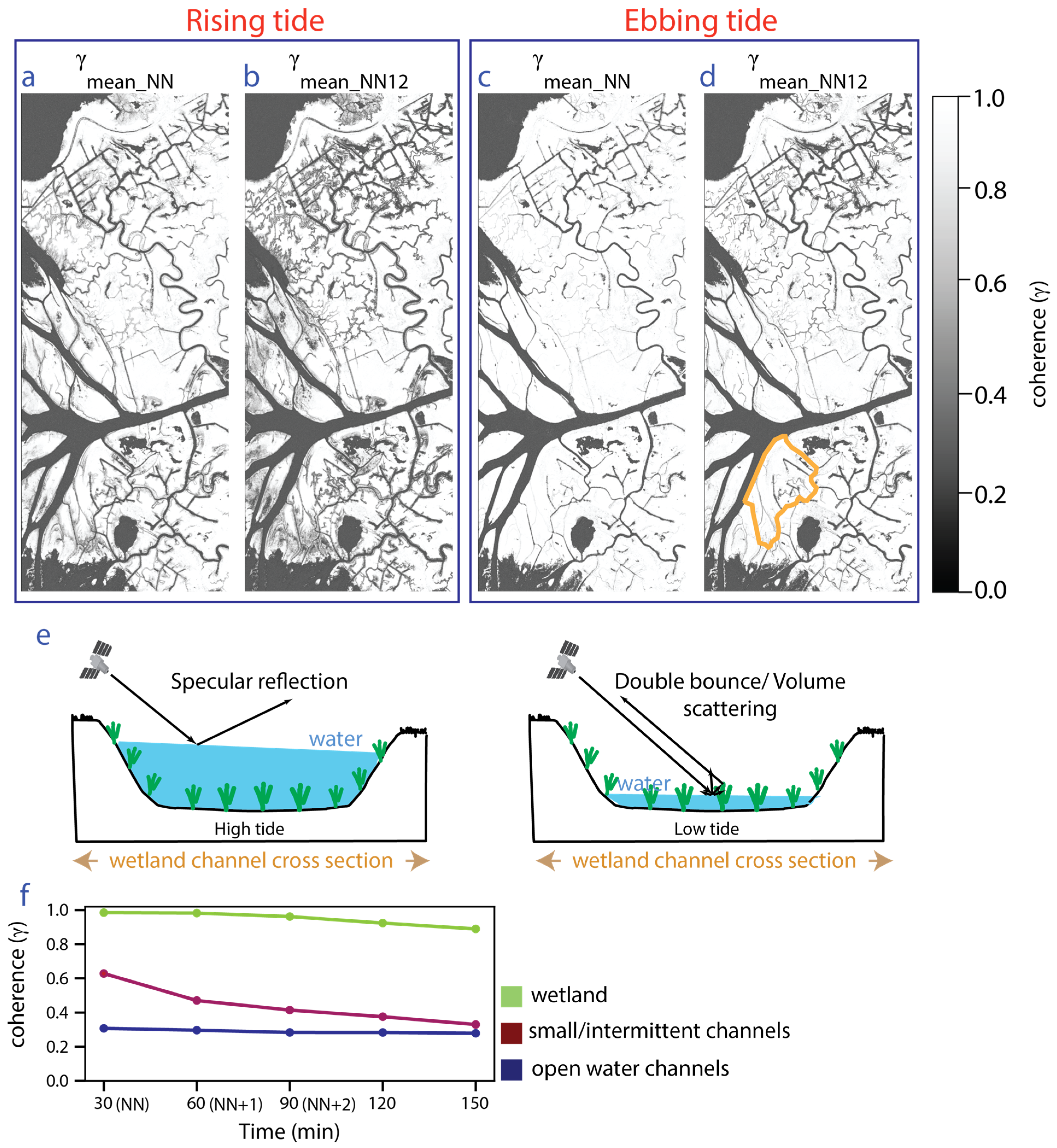
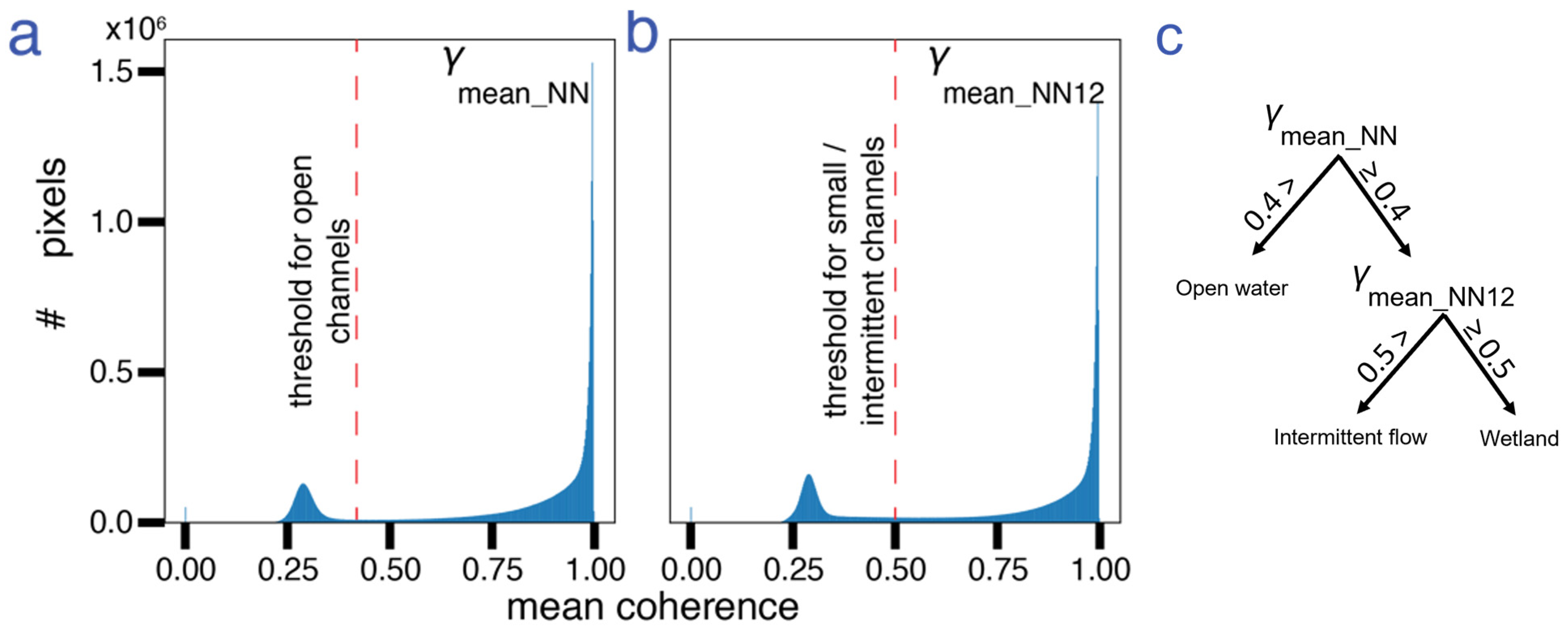

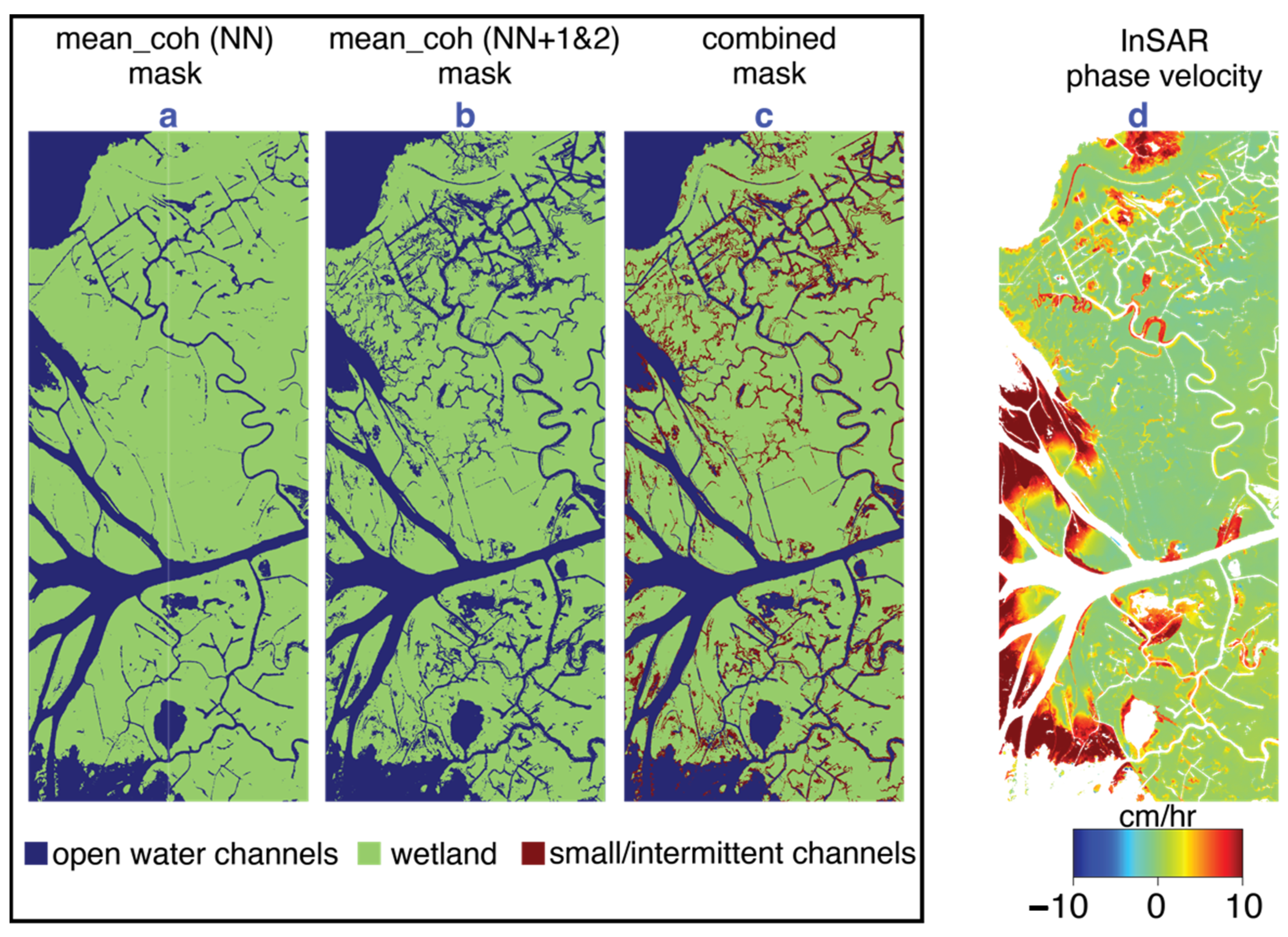
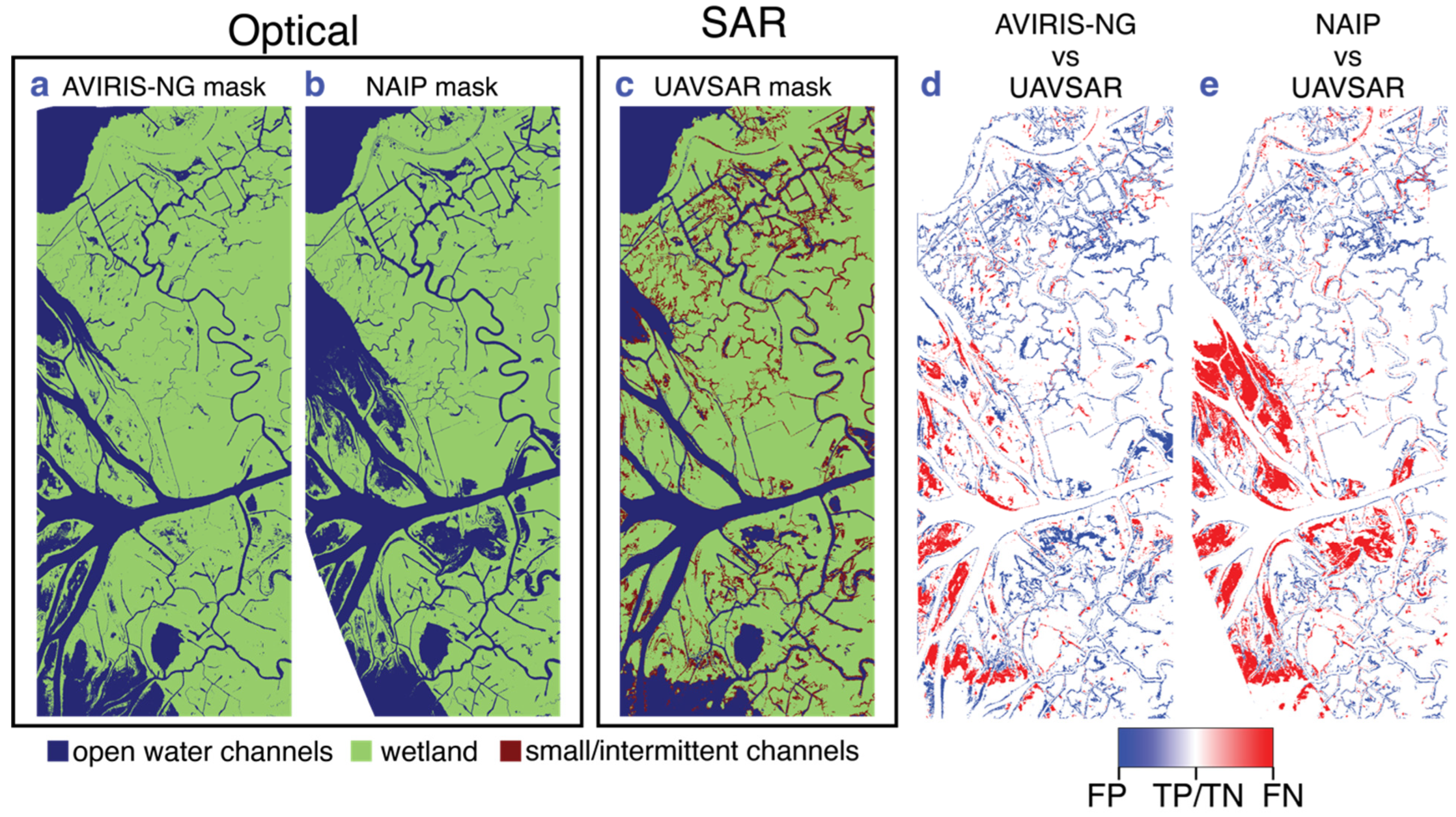
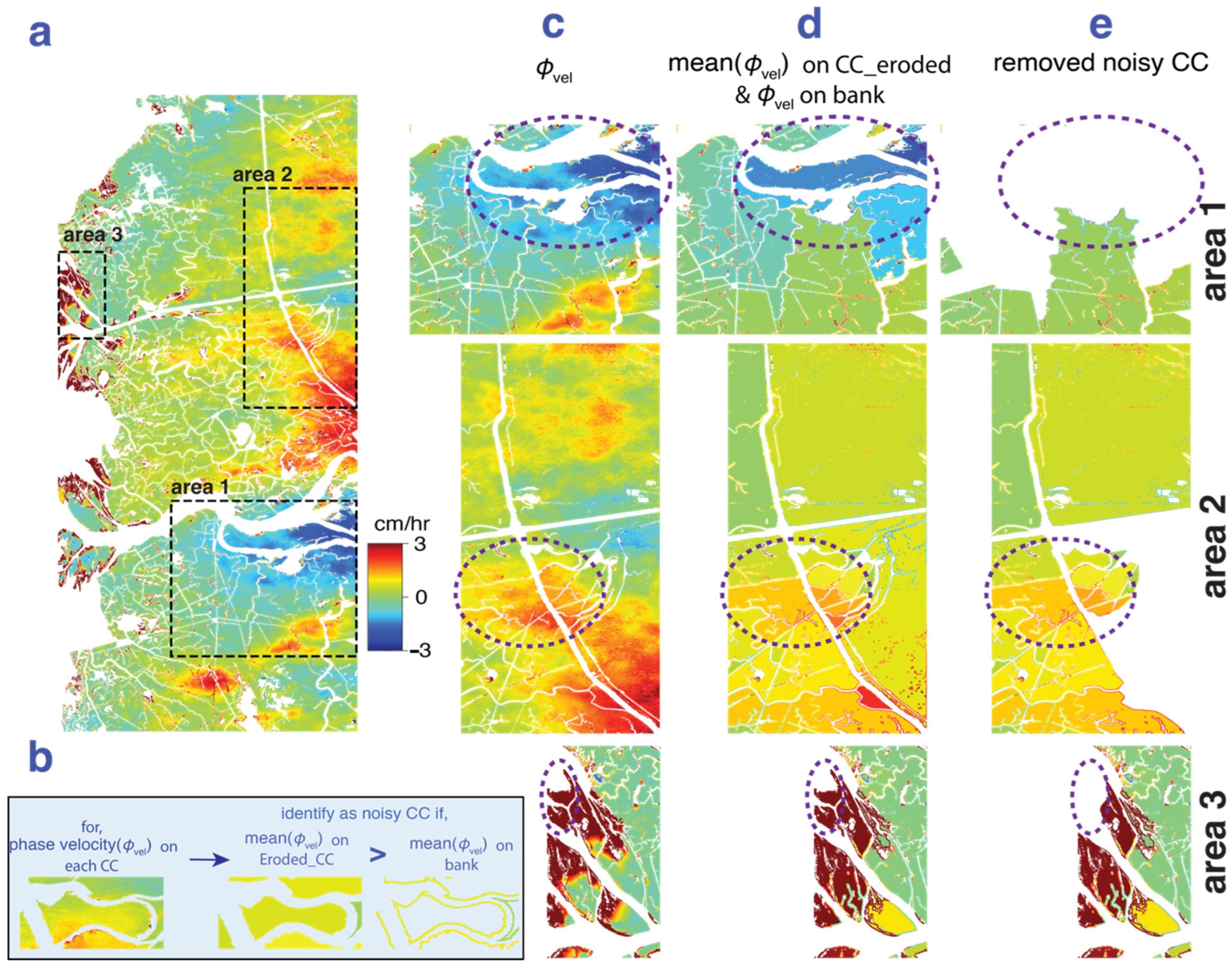

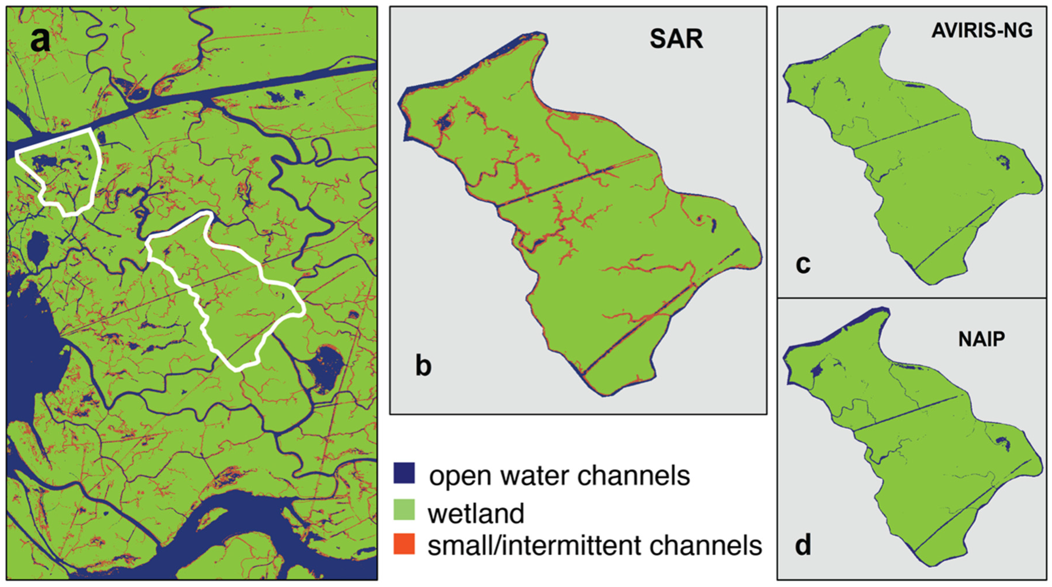
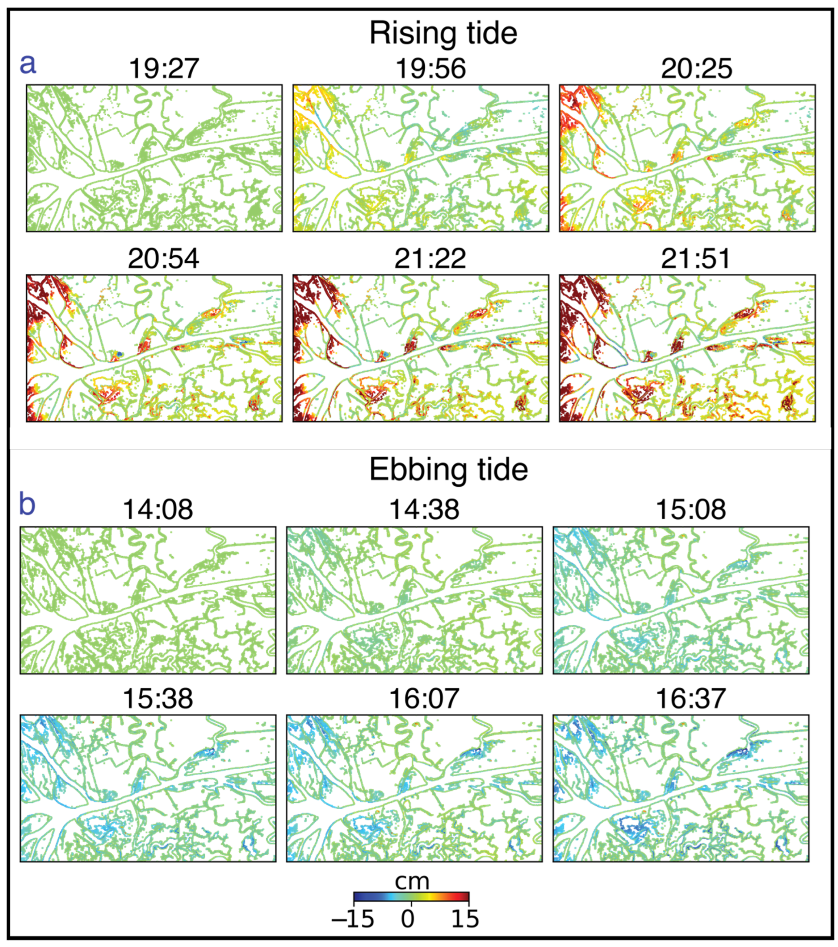
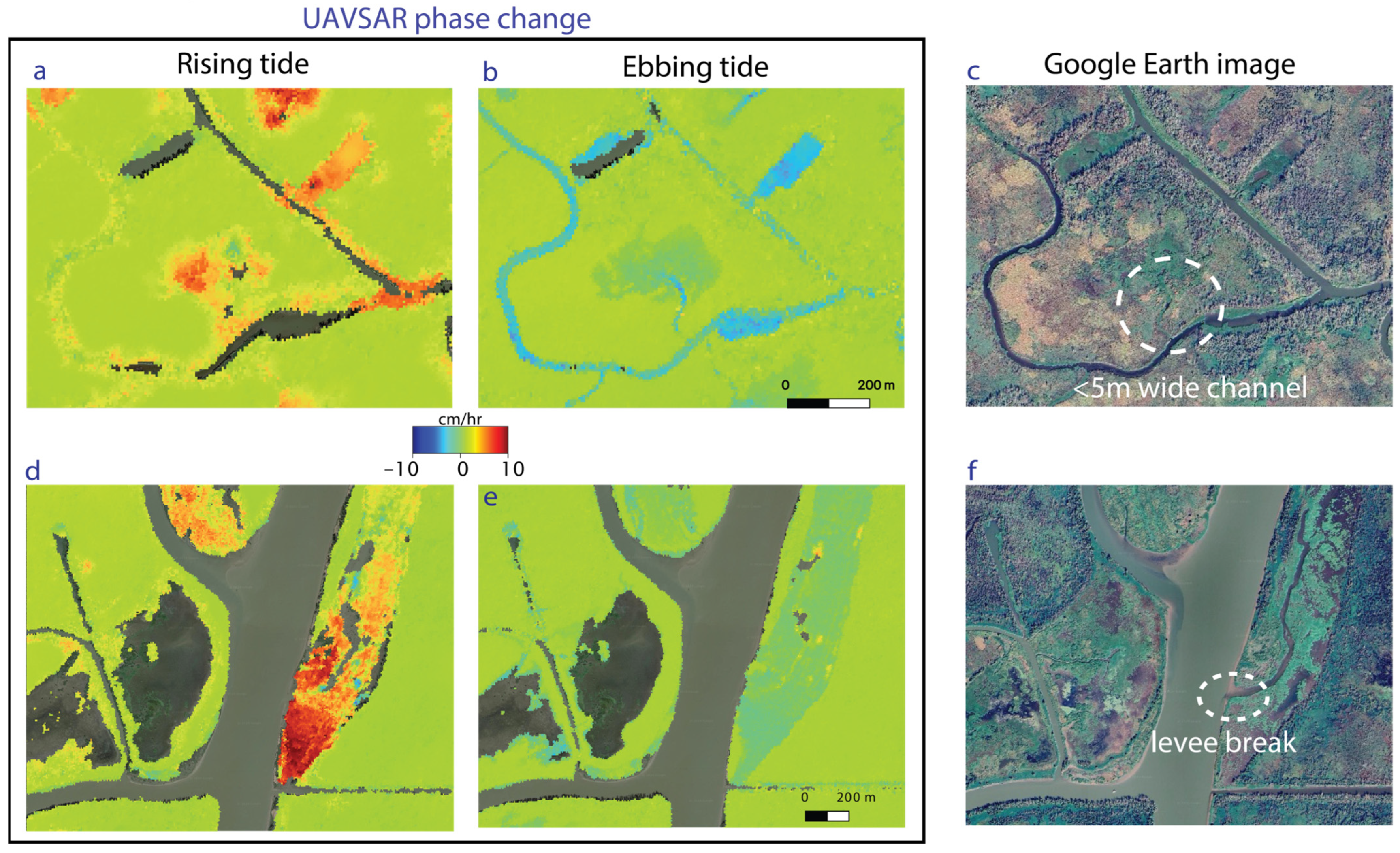
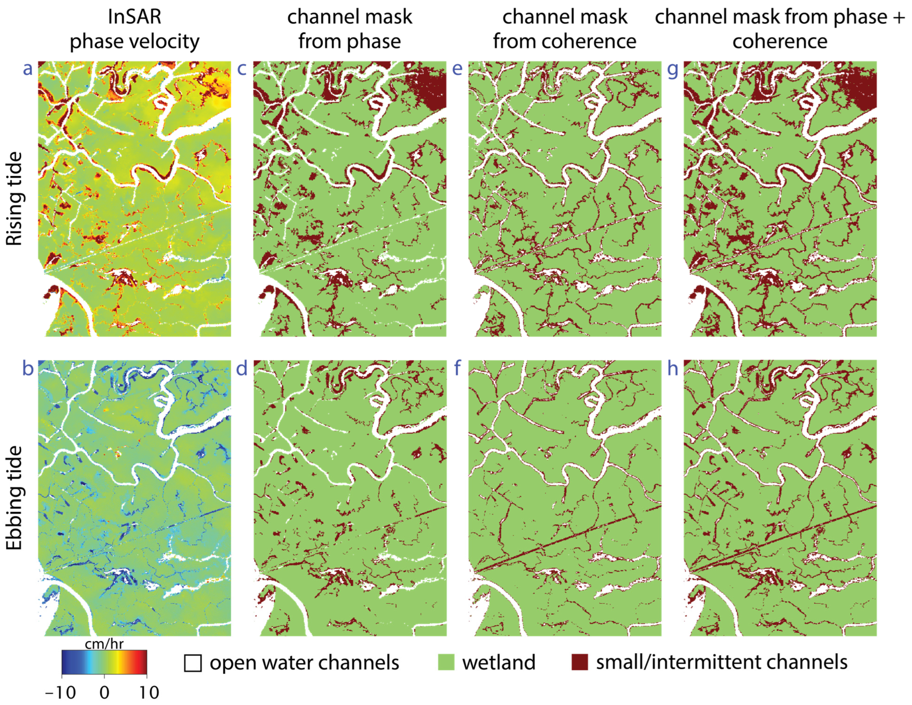
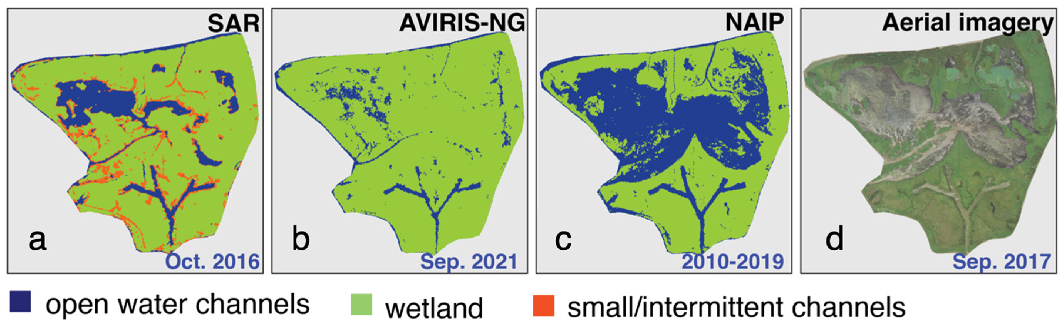
Disclaimer/Publisher’s Note: The statements, opinions and data contained in all publications are solely those of the individual author(s) and contributor(s) and not of MDPI and/or the editor(s). MDPI and/or the editor(s) disclaim responsibility for any injury to people or property resulting from any ideas, methods, instructions or products referred to in the content. |
© 2025 by the authors. Licensee MDPI, Basel, Switzerland. This article is an open access article distributed under the terms and conditions of the Creative Commons Attribution (CC BY) license (https://creativecommons.org/licenses/by/4.0/).