ACCURACy: A Novel Calibration Framework for CubeSat Radiometer Constellations

Abstract

As a result of progress in space technology, more scientific missions are benefiting from using CubeSats equipped with radiometers. CubeSat constellations are especially effective in overcoming obstacles in cost, weight, and power. However, these benefits have certain significant downsides, including the difficulty in calibration due to the increased sensitivity of instruments to ambient conditions. Such limitations prevent conventional calibration methods from being reliably applied to CubeSat radiometers. A novel, constellation-level calibration framework called “Adaptive Calibration of CubeSat Radiometer Constellations (ACCURACy)” is being developed to address this issue. ACCURACy, in its current version, uses telemetry data obtained from thermistors in each CubeSat to cluster constellation members into time-adaptive groups of radiometers in similar states. Each radiometer is assigned membership to a cluster and this status is updated as in-orbit measurements shift in the clustering model. This paper introduces the ACCURACy framework, discusses its theoretical background, and presents a MATLAB prototype with performance and uncertainty analyses using synthetic radiometer data in comparison with traditional radiometer calibration methods.

1. Introduction

The rapid developments in space technologies have enabled a wide range of applications of CubeSats in radiometry missions. The calibration and intercalibration of traditional radiometers in constellations are often performed by using stable radiometers calibrated using vicarious targets or radiative transfer models (RTMs) as reference and using the post-processing of constellation measurements to identify and eliminate biases between the constellation members and those references [1,2,3,4,5,6]. CubeSats provide a lighter, cheaper, and lower-power alternative to traditional systems; but increased sensitivity to ambient conditions due to their lower thermal mass and lack of radiation shielding makes real-time calibration challenging for CubeSat radiometers. Moreover, size and mass limitations may restrict use of blackbody targets. Due to their small size (typically 10 cm × 10 cm × 10 cm for a 1U CubeSat) and limited mass (up to 1.33 kg per unit for a 1U), incorporating larger or heavier components like blackbody targets into CubeSats is challenging, as these require space for effective thermal radiation uniformity. For instance, a typical blackbody target with a diameter of 33 cm is too large to fit on a typical 3U CubeSat [7,8]. Additionally, maintaining the stability and performance of noise diodes and matched loads, which require precise temperature control, endurance, low-noise floor, and low return losses, is difficult in the variable conditions of space due to the limited resources for thermal and power management, which may prevent the use of noise diodes and matched loads as calibration references in CubeSats [9,10,11]. Thus, errors and uncertainties associated with the calibration of individual CubeSat radiometers, which must exploit infrequent measurements of external targets, can be significant and no single instrument or RTM can be utilized as a calibration reference within a constellation of CubeSats as measurements of calibration references should be precise and stable. Therefore, a novel constellation-level calibration method is required. To address this gap, a framework called “Adaptive Calibration of CubeSat Radiometer Constellations” (ACCURACy) is being developed as a traceable, quantifiable, real-time system-level calibration of CubeSat radiometer constellations [12,13,14,15,16]. An analysis of IceCube, a 3U CubeSat developed at the NASA Goddard Space Flight Center for a spaceflight demonstration of an 883 GHz radiometer, has presented radiometer gain and offset as a function of the physical temperature of the satellite measured by thermistors and the age of the instrument [17]. This relationship is the core component of ACCURACy since it can be used to characterize the state of a radiometer and identify radiometers in similar states to share their calibration data. ACCURACy has been developed into a working prototype on MATLAB using synthetic data modeling; Figure 1 shows the main monitoring panel of ACCURACy while in operation. Over the course of this paper, we review the current state-of-the-art (SOTA) methods used for intercalibration of radiometer constellations in the SOTA Intercalibration section, introduce and dissect the ACCURACy framework in the methodology section, go through ACCURACY, SOTA, and ideal calibration simulations in the results section, and analyze the performance of ACCURACy, compared to the other two calibration cases in the discussion section. Finally, we end with discussing the future plans for the further development of ACCURACy.

2. SOTA Intercalibration

Satellite intercalibration is a challenging task, and the current state-of-the-art techniques have been in development since the 1980s. This began with the calibration and validation studies performed by the Space Sciences Division of the Naval Research Laboratory on the first Special Sensor Microwave Imager (SSM/I), primarily to establish an absolute calibration and investigate instrument sensitivity [18,19]. Currently, one of the most significant examples of intercalibrating constellations of radiometers is the NASA Global Precipitation Measurement Mission (GPM) [20,21,22]. The GPM Intersatellite Calibration Working Group (X-CAL) is a group of several teams from different institutions and universities tasked with developing methods to make the radiometric calibrations consistent between GPM constellation radiometers [23,24]. X-CAL team uses the GPM Microwave Imager (GMI) instrument as a transfer standard between radiometers in the GPM constellation. GMI has proved, thus far, to be very stable and to be able to maintain a very good calibration due to its dual calibration procedure, which includes an external cold space and an internal hot blackbody and noise diode measurements [21,25]. Adjustments based on GMI are applied with respect to the different frequencies, polarizations, and view angles, and use observations from pairs of satellites at nearly the same times and locations in a one-degree latitude/longitude grid.

In this study, an intercalibration method, which uses observations from pairs of satellites at nearly the same times and locations, mimicking the GPM intercalibration procedure [5], is developed and called the state-of-the-art (SOTA) intercalibration. SOTA is implemented via overlapping calibration measurements, performed by different radiometers, over the same 1⁰ × 1⁰ latitude x longitude grid cells on the Earth’s surface, within one minute. The calibrated products of individual radiometers, following the standard least-squares-regression based approach described in Section 3.2.3, are corrected by the most recent measurements to eliminate the inconsistencies among the constellation members. The previously mentioned challenges associated with SOTA intercalibration applied to CubeSats due to their lower stability and higher sensitivity to ambient conditions, compared to traditional monolithic systems [26], and how ACCURACy addresses them are discussed in the following sections.

3. Methodology: ACCURACy Framework

ACCURACy is a novel approach for intercalibrating constellations of identical radiometers which may individually be unable to maintain a precise absolute calibration on their own. It is structured into three modules, which form a real-time processing loop: the clustering module, which processes the incoming telemetry data stream from constellation members and gathers them into clusters of similar state radiometers to share their calibration data among the other cluster members; the calibration pool module, which updates pooled calibration measurements shared between the constellation members and eliminates data from unhealthy instruments; and the calibration module, which produces calibrated antenna temperatures for each radiometer in the constellation through a least-squares-regression based algorithm, using the available calibration data pool.

ACCURACy can either run using real-time data streams or can be used in a post-processing mode to process data and return calibrated measurements in batches. Figure 2 depicts an overall diagram of the framework and its modules, as well as the flow of data through each module, with data inputs and outputs at each state.

3.1. Radiometer Gain Characteristics: Theoretical Background

The clustering module of ACCURACy leverages the relationship between the receiver gain and offset, and the physical temperature of the instrument. As shown in [27], the gain of the IceCube radiometer can be modeled as a function of payload temperature, as well as the gain’s drift over time. This relationship forms the basis for the clustering module of ACCURACy.

The telemetry dataset used by ACCURACy is composed of a set of measurements from each of the thermistors on each satellite. These data describe the physical temperature of a satellite at a given time (payload temperature, (Tp)). Tp is a function of thermal effects from external (i.e., the sun) and internal (i.e., electronic components) sources; although, this is assumed to be a simple sinusoid, and the instrument is power cycled to maintain the equilibrium.

So, the output for each thermistor on a CubeSat is modeled as a sinusoidal (e.g., representing heat from the sun, as the satellite moves in its orbit) in time with statistical noise due to the system noise of the instrument and is expressed as:

$${\widehat{Th}}_{rk}\left(t\right)=A\times sin\left(\omega t+{\theta }_r\right)+N\left(t\right),$$

(1)

where ${\widehat{Th}}_{rk}$ is the normalized output of the kth thermistor on the rth radiometer of the constellation, ${\theta }_r$ is a phase offset for the radiometer at the start of the constellation operation, $N\left(t\right)$ is a random noise added to each thermistor, constant $A$ is the normalized amplitude, and $t$ is time.

Mimicking the IceCube radiometer, ACCURACy assumes that the thermistor data for each satellite determines its gain process. To model this relationship, the radiometer gain in time can be expressed as a weighted sum of the thermistor measurements and their change over time (e.g., warming up vs cooling down), as well as the age of the instrument, as in the following equation:

$$g_r\left(t\right)={\sum }_{k=1}^N{W}_{rk}{\widehat{Th}}_{rk}\left(t\right)+W_{rt}{t}_r+\Delta {\widehat{Th}}_{rk}\left(t\right),$$

(2)

where $g_r$ and $t_r$ is the gain and age of the rth radiometer, respectively, $W_{rk}$ is the weight associated with the kth thermistor on the rth radiometer, $W_{rt}$ is the weight associated with the age of the rth radiometer, and $\Delta {\widehat{Th}}_{rk}$ is the temperature gradient factor for the kth thermistor on the rth radiometer representing different gain characteristics during warming and cooling periods of the radiometer.

The random noise in the thermistor data, $N(\sigma ,\overline{X})$ in Equation (1), can be modeled on an arbitrary first order autoregressive process, AR(1), as radiometers, in steady state conditions, are typically assumed to be stationary, but are generally wide-sense stationary. Thus, the radiometer gain noise generated using an AR(1) process with two parameters can be described by:

$$\mathrm{N}\left(t\right)={\mathsf{\beta }}_0+{\mathsf{\beta }}_1\mathrm{N}\left(\mathrm{t}-1\right)+{\mathsf{ϵ}}_{\mathrm{g}},$$

(3)

where ${\in }_g~N\left(0,{\sigma }_{ϵ}\right)$ is gaussian noise and ${\mathsf{\beta }}_1$ is the first order correlation coefficient. The constant ${\beta }_0$ can be considered the mean of the process, resulting in a zero-mean AR(1) process defined simply by:

$$\mathit{N}\left(\mathit{t}\right)={\mathsf{\beta }}_1\mathrm{g}\left(\mathrm{t}-1\right)+{\mathsf{ϵ}}_{\mathrm{g}},$$

(4)

$$\mathrm{N}\left(0\right)=0.$$

(5)

A radiometer system with a gain defined by Equation (2) produces voltage counts in time that can be expressed with the following simple equation:

$$C_r\left(t\right)=g_r\left(t\right)\times T_b\left(t\right)+C_{ro}\left(t\right),$$

(6)

where $C_r$ is the voltage count of the rth radiometer, $T_b$ is the brightness temperature of the measurement, and $C_{ro}$ is the background count/offset.

Note that the current theoretical basis of the ACCURACy framework regarding the relationship between the CubeSat telemetry data and radiometer gain properties will be subject to further study and characterization, using data from operational CubeSat radiometer constellations such as “Time-Resolved Observations of Precipitation structure and storm Intensity with a Constellation of Smallsats” (TROPICS) [28,29], as they become available to the authors.

3.2. ACCURACy Modules

As previously mentioned, ACCURACy is divided into three modules, the clustering module, the calibration pool module, and the calibration module. The following subsections provide detailed descriptions of each module.

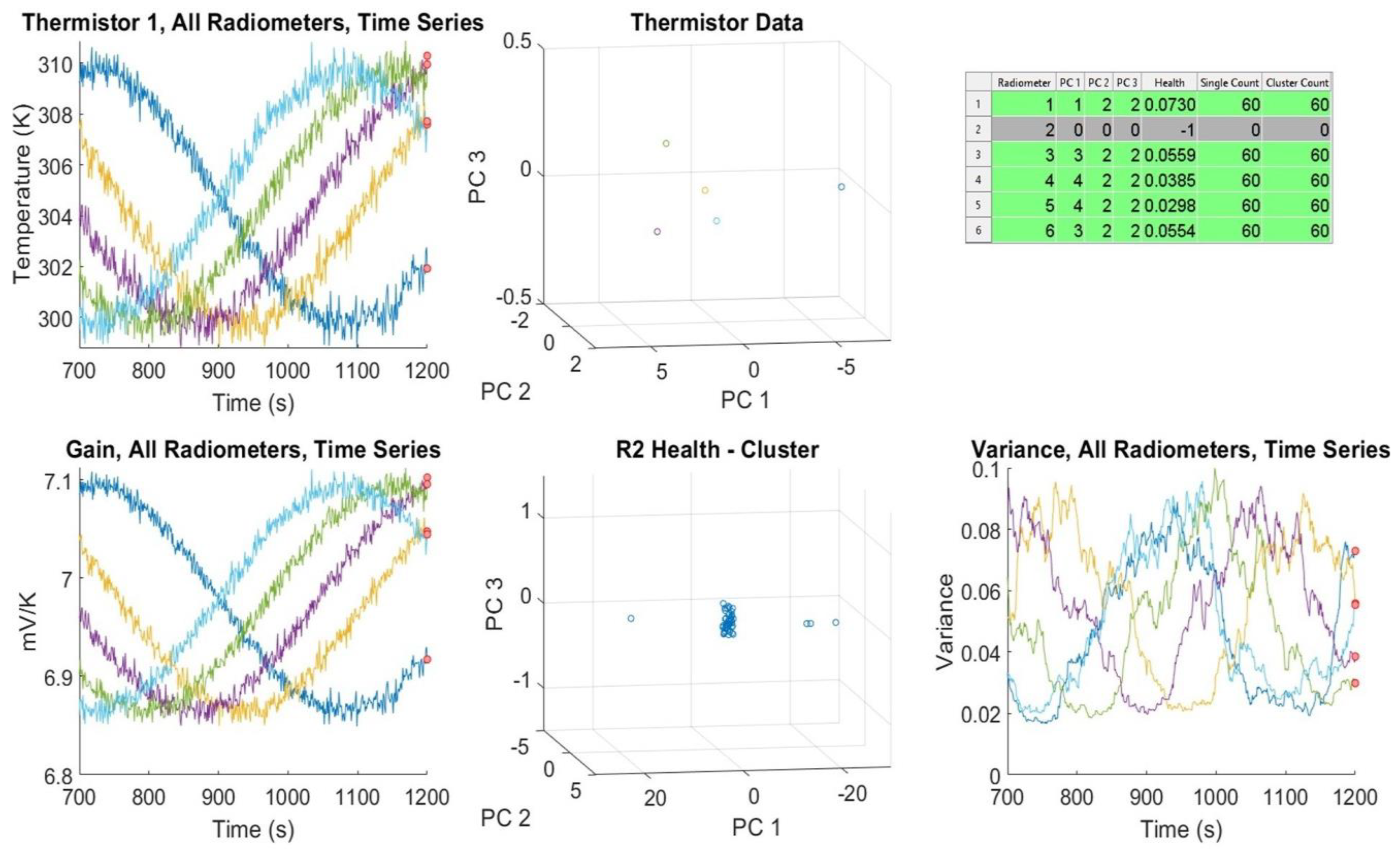
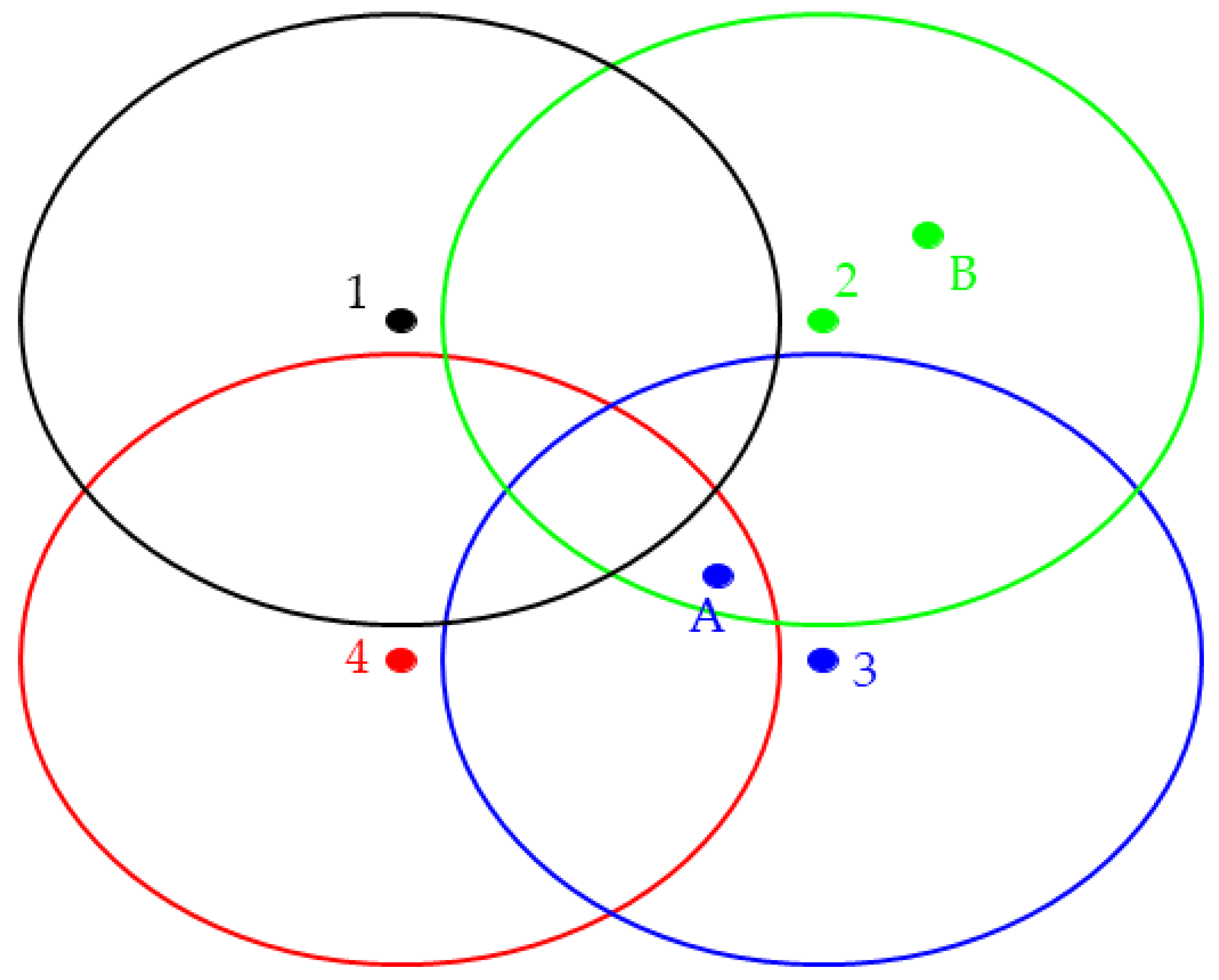
3.2.1. Clustering Module

The clustering module performs two main tasks: first, the processing of incoming telemetry data by using and normalizing dimensionality reduction techniques, and second, establishing time-adaptive clusters for all of the radiometers in the constellation and assigning them time variable cluster labels, using up-to-date, instrument-level telemetry data.

Incremental Principal Component Analysis (PCA) is used to reduce dimensionality by calculating the principal components of the data: the n-best fit and orthogonal unit vectors for an n-dimensional set of points. The principal components of the telemetry dataset are the eigenvectors of the covariance matrix of the data [30]. The second step of the PCA is to use the eigenvectors of the dataset to perform a change of basis on the data. This ensures that the ith feature, i.e., dimension, of the resulting transformed data, is the feature containing the ith highest variance among all features, wherein the features are organized in descending order according to the corresponding eigenvalues. Dimensionality reduction is performed by identifying the k eigenvectors accounting for a sufficient amount of the total explained variance in the telemetry dataset. For ACCURACy, k eigenvectors are chosen, so that 75% of the variance in the data is explained by those k eigenvectors; however, this threshold is variable, based on calibration accuracy requirements. This is conducted by organizing the eigenvectors in a descending order according to the associated eigenvalues, and choosing the first k eigenvectors:

$$0.75\le {\displaystyle \frac{{\sum }_{\mathrm{i}=1}^{\mathrm{k}}{\mathsf{\lambda }}_{\mathrm{i}}}{{\sum }_{\mathrm{j}=1}^{\mathrm{n}}{\mathsf{\lambda }}_{\mathrm{j}}}}.$$

(7)

Dimensionality reduction is used in ACCURACy to reduce the computational load, and to extract the features which account for the sufficient variability in the data, so that there is no substantial error introduced in the subsequent clustering. Figure 3 shows the proportion of the explained variance retained in the data as additional principal components are included in a sample set of calibration data from a simulation of the ACCURACy framework in operation. In this example, 75% of the explainable variation in the data is chosen as a threshold; therefore, k is chosen to be 3.

The goal of the clustering module is to identify which radiometers are in similar states at a given time. Data is classified using a clustering algorithm. For each CubeSat radiometer in the constellation of n members, the clustering module maintains an up-to-date n-dimensional telemetry data vector of instrument-level thermistor readings. These data are used by the clustering module to cluster radiometers based on similar states. Furthermore, radiometers should be able to be matched with the calibration measurements made by similar state radiometers in the past. So, the clustering module must implement an algorithm or procedure which can, at a given time, for a given radiometer, find all the past calibration measurements which were made by a radiometer in a similar state to the state the current radiometer is in.

Several candidate clustering algorithm families were identified as possible solutions for the clustering module. Density-based spatial clustering of applications with noise (DBSCAN) was the first clustering algorithm considered for use [31]. However, a few downsides were discovered in the course of development, which limit its usefulness in ACCURACy. First, looking at a continuous stream of data in time, a density-based algorithm may see the data as one connected dense region. Second, DBSCAN has a high computational cost which is not desirable for a real- time calibration scenario. Another version of DBSCAN was also implemented using time as an additional dimension. This method also gave poor results due to DBSCAN’s bias towards globular clusters.

These problems are circumvented by cell-based clustering algorithms, in which the entire data space is first separated into separate, i.e., normal, or overlapping clusters, and then data points are placed into the space. This type of clustering algorithm also has a low computational cost, which is a good fit for ACCURACy, since clustering ideally needs to be performed onboard, in real-time, to promptly react to critical observations the constellation may perform, instead of implementing recalibration through ground processing, long after the measurements are made.

Using overlapping cell-based clustering, a space describing all possible radiometer states is filled with spheres that represent individual clusters, as demonstrated in Figure 4. To cover the entire space, the clusters must overlap. The cluster centers are laid out on a lattice. Due to the spheres overlapping, a radiometer in a specific state will fall into one or more of these clusters. The radiometer will store its calibration information in every cluster it belongs to. A new radiometer will be calibrated using a least-squares regression of the calibration data, stored in the cluster whose center it is the closest to.

The incremental DBSCAN, a modified version of the DBSCAN in which one point is clustered at a time and added to the core points of previously clustered data, also shows improvement over traditional DBSCAN methods [32,33]. In the incremental DBSCAN, a new point will become a member of the closest cluster to it, as long as the new point falls within a certain radius of its center. If it is not within one radius distance to any cluster center, it creates a new cluster and becomes the center of that new cluster.

A figure of merit is defined to evaluate the performance of different clustering algorithms by calculating the average distance from the cluster center to all points in that cluster for all clusters:

$${\mathrm{M}}_{\mathrm{a}\mathrm{v}\mathrm{g}}={\displaystyle \frac{1}{\mathrm{N}}}{\sum }_{\mathrm{i}=1}^{\mathrm{k}}{\sum }_{\mathrm{j}=1}^{\mathrm{n}}\left|\right|{\mathrm{P}}_{\mathrm{i},\mathrm{c}\mathrm{e}\mathrm{n}\mathrm{t}\mathrm{e}\mathrm{r}}-{\mathrm{P}}_{\mathrm{i},\mathrm{j}}{\left|\right|}_2,$$

(8)

where N is the total number of points in all clusters, k is the number of clusters, n is the number of points in a cluster, and $|{|P}_{i,center}-P_{i,j}{\left|\right|}_2$ is the Euclidian distance between $P_{i,center}$, the centroid of cluster i and $P_{i,j},$ the $j^{th}$ point in cluster i. This figure of merit will be referred to as the Mean Distance from Centroid (MDC). The MDC provides a measure of the average density of points for the clusters created using each algorithm— this metric is often used in evaluating k-means clustering methods [34].

Table 1. Clustering algorithms investigated for ACCURACy and their MDC values.

Clustering Method	MDC
DBSCAN	3.3939
Incremental DBSCAN (IDBSCAN)	0.6849
Overlapping Cell-Based	0.5115
Normal Cell-Based	2.1172

lists the average MDC values for all clustering algorithms considered for ACCURACy, over one hundred simulations of a constellation of 35 CubeSats, under various conditions, for 50 s.

Figure 5 shows the clusters created by DBSCAN, IDBSCAN, as well as separate and overlapping cell-based clustering, with each cluster represented by a different color for one of the sample constellation telemetry datasets processed by ACCURACy, to calculate the MDC values listed in Table 1. The spread of points within the clusters for each of the four clustering algorithms are also depicted in the figure.

DBSCAN, as shown in Figure 5 (top left), performs rather poorly at identifying the different gain states, as defined by different clusters. This is likely due to its strong ability at identifying dense, connected regions of points, which becomes a flaw in this scenario, where data are continuously generated, spanning across the data space. IDBSCAN performs fairly well, as it can respond to changes in data structure over time. In simulation, overlapping cell-based clustering minimizes within-cluster distance, resulting in clusters with the most similar points.

Each algorithm is also evaluated based on the quality of the calibration when used within the ACCURACy framework. Two metrics are used to evaluate the overall calibration performance of ACCURACy: first, the root-mean-square error (RMSE) compared to the true measurand brightness temperature, and second, the variance of the resulting calibration, compared to the radiometric sensitivity. Both metrics are used in evaluating ACCURACy with different clustering algorithms for the clustering module. The best performance was again seen using the overlapping cell-based clustering. This approach is similar to the SOTA intercalibration method, described previously in Section 2, which identifies calibration measurements taken by two constellation members at nearly the same location and time. The significant advantage of using ACCURACy is that the framework enables us to identify similar state radiometers for calibration data sharing at different points in time and different locations. Moreover, instead of correcting the calibrated measurements in most SOTA methods, ACCURACy preserves the individual calibration of constellation members.

Several other data processing methods have also been tried for the clustering module to identify similar state radiometers. One of them uses the weighted locations of telemetry data in the principal component space. This method does not use clustering; instead, a collection of recent, e.g., last 5 min, telemetry data points are saved, and radiometers use every previous saved calibration point associated with them for calibration. Instead of clustering points from radiometers in similar states together, each telemetry data point is assigned a weight, expressed as follows, based on how similar the state of the radiometer was to the current state:

$${\mathrm{W}}_{\mathrm{j}}={\left(\sum {\mathrm{P}}_{\mathrm{i}}-{\mathrm{P}}_{\mathrm{j}}\right)}^{-1/2},$$

(9)

where ${\mathrm{P}}_{\mathrm{i}}$ and ${\mathrm{P}}_{\mathrm{j}}$ represent the location of ith and jth telemetry data point in the principal component space, and the weight, ${\mathrm{W}}_{\mathrm{j}}$, is used when the calibration data corresponding to the jth telemetry reading to calibrate the radiometer with ith telemetry data point. This process is repeated for all new points. The method of weighted locations was chosen because it was highly resistant to noise and since the radiometers never had to change clusters, the resulting calibration was smoother than most other clustering methods. On the other hand, calibration accuracy analyses, similar to those performed for the four clustering methods, indicated poorer results.

After performance analyses of all the algorithms considered for ACCURACy, the overlapping cell-based clustering algorithm has been selected as the default option for the clustering module. On the other hand, other options are also coded in the framework and switching from one method to another is possible. Finally, note that all algorithms produce time-adaptive clusters, which means that as new telemetry datasets are processed, the cluster labels of the radiometers are updated accordingly.

3.2.2. Calibration Pool Module

The calibration pool module forms calibration data pools from cluster labels, calibration measurements, and times provided from the clustering module. The calibration pool for each cluster is used to estimate the gain and offset for that cluster so that each radiometer in the cluster can be calibrated accordingly. The result is a real-time, multi-point absolute calibration opportunity for each radiometer in the constellation.

The calibration pool module implements standard algorithms and data structures to manage the calibration data associated with all clusters. There is currently no need to develop special techniques or methods for managing calibration pools. As new telemetry and calibration data arrive, the calibration pool module is updated with a new set of cluster labels for all radiometers from the clustering module. Each radiometer is checked to see if any new calibration measurements have been made. If so, these new calibration measurements are saved with the cluster labels. Then, the calibration pools are updated with this new data. Calibration data stored in the pools are independent of their measurement location and time, as long as they come from radiometers within the same cluster, thus the number and frequency of calibration measurements available to each radiometer in the ACCURACy framework are usually higher than those in the SOTA intercalibration described in Section 2.

The calibration pool module also monitors the health of each radiometer by tracking the variance of the telemetry data. If the mean variance of the telemetry data, i.e., thermistor readings, exceeds a certain threshold for a radiometer over a specific window, that radiometer is flagged as unhealthy and removed from the ACCURACy processing. Equation (10) below expresses this condition mathematically:

$${\displaystyle \frac{1}{\mathrm{N}}}{\sum }_{\mathrm{k}=1}^{\mathrm{N}}\mathrm{v}\mathrm{a}\mathrm{r}\left\{{\widehat{Th}}_{rk}\left(∆{\mathrm{t}}_{\mathrm{h}}\right)\right\}>\mathrm{t}\mathrm{h}\mathrm{r}\mathrm{e}\mathrm{s}\mathrm{h}\mathrm{o}\mathrm{l}\mathrm{d}$$

(10)

where $\mathrm{N}$ is the number of thermistors on a radiometer, $∆{\mathrm{t}}_{\mathrm{h}}$ is the preset time window for health check and threshold is the health threshold. Figure 6 demonstrates an example where a single radiometer in the constellation becomes unhealthy during the operation and is flagged by the calibration pool module of ACCURACy.

3.2.3. Calibration Module

To perform the actual calibration, the calibration module communicates with the calibration pool module to retrieve calibration data including voltages, reference temperatures, and observation times from the calibration pools respective to each radiometer. Then, calibration data associated with each cluster is used to calibrate all radiometers within those clusters.

The calibration modules perform calibration using standard least-squares-regression expressed as:

$$\widehat{{\mathrm{T}}_{\mathrm{A}}}=\left(V_A-{〈V_i〉}_n\right){\displaystyle \frac{{\sum }_{\mathrm{i}=1}^{\mathrm{n}}\left(V_i-{〈V_i〉}_n\right)T_i}{{\sum }_{\mathrm{i}=1}^{\mathrm{n}}{\left(V_i-{〈V_i〉}_n\right)}^2}}+{〈T_i〉}_n,$$

(11)

where $\widehat{{\mathrm{T}}_{\mathrm{A}}}$ is the estimated antenna temperature, i.e., calibrated radiometer product associated with the measurement target (e.g., Earth’s atmosphere, planetary surface, etc.), $V_A$ is the antenna voltage, i.e., the receiver output voltage when the radiometer is observing that target, $V_i$ and $T_i$ are the receiver output voltages and antenna temperatures associated with the ith calibration reference (e.g., cold space, ocen surface, etc.), and ${〈V_i〉}_n$ and ${〈T_i〉}_n$ are the average of those voltages and temperatures of the $n$ number of observed calibration references [35].

ACCURACy is also able to mathematically quantify the errors and uncertainties in calibration products. First, the uncertainty, i.e., variance in the estimated antenna, which is defined as:

$${{\mathsf{\sigma }}^2}_{{\widehat{\mathrm{T}}}_{\mathrm{A}}}=\mathrm{E}\left\{{\left({\widehat{\mathrm{T}}}_{\mathrm{A}}-{\overline{\mathrm{T}}}_{\mathrm{A}}\right)}^2\right\},$$

(12)

Can be analytically calculated as follows, if the gain process is following an autoregressive process as mentioned in Section 3.1:

$${{\mathsf{\sigma }}^2}_{{\widehat{\mathbf{T}}}_{\mathbf{A}}}={\sum }_{\mathit{i}=1}^{\mathit{K}}{\mathit{\sigma }}_{{\mathit{x}}_{\mathit{i}}}^2{\mathit{f}}_{{\mathit{x}}_{\mathit{i}}}^2+2{\sum }_{\mathit{i}<\mathit{j}}{\mathit{f}}_{{\mathit{x}}_{\mathit{i}}}{\mathit{f}}_{{\mathit{x}}_{\mathit{j}}}\mathit{c}\mathit{o}\mathit{v}\left({\mathit{x}}_{\mathit{i}}{\mathit{x}}_{\mathit{j}}\right),$$

(13)

where

$$f_{x_i}={\left.{\displaystyle \frac{\mathsf{\partial }}{\mathsf{\partial }{x}_i}}f\left(x_1,x_2,\dots ,x_k\right)\right|}_{x_1=\overline{x_1},\dots ,x_k=\overline{x_k}},$$

(14)

and $x_i$ and $x_j$ represent the parameters in the calibration equation, i.e., Equation (11), ${\sigma }_{x_i}^2$ is the inherent variance associated with the parameter $x_i$, and $f$ is the function representing the least-squares-regression as:

$$\widehat{{\mathrm{T}}_{\mathrm{A}}}=f\left(x_1,x_2,\dots ,x_k\right).$$

(15)

The result is a comprehensive definition of uncertainty, which includes radiometric resolution, i.e., noise equivalent delta temperature of the radiometer, and uncertainties associated with calibration measurements, allowing ACCURACy to establish measurement traceability, and assess calibration accuracy, sensitivity, and stability [36,37]. Large numbers of calibration measurements will also enable checking for any calibration drifts and their impacts on the calibrated products by calibrating one vicarious calibration reference target using the remaining calibration measurements as explained in [38].

4. Results: Initial Experiments

4.1. Data Generation

The overarching goal in developing ACCURACy is to enable the complete intercalibration of all satellites within a constellation of CubeSat radiometers in real-time. It is necessary to continuously test and improve the framework in the course of its development, which requires a dataset describing the conditions under which ACCURACy may be deployed. There are currently a few planned collaborations to test ACCURACy on real data collected from constellations of CubeSats. One such collaboration will be in conjunction with MIT Lincoln Laboratory, using data from the “Time-Resolved Observations of Precipitation Structure and Storm Intensity with a Constellation of SmallSats (TROPICS)” mission [28,29]. However, until the studies with those data can be performed, synthetic datasets must be generated in order to perform any testing. To this end, a module has been developed to generate synthetic orbit and calibration data for a constellation of CubeSats.

The simulated dataset is composed of three portions:

• A dataset describing the orbital mechanics,
• A telemetry dataset, and
• A calibration dataset, for all radiometer carrying satellites in the constellation.

Figure 7 shows how these datasets are used to generate the overall synthetic radiometer data. The orbits of each CubeSat are described by a set of orbital planes that each consists of a set of inclination angles (phi and theta) and the number of satellites that exist along it. Simulating the satellite orbits in this way allows the simulation to mimic different data collection scenarios, since different scientific missions may have different objectives, e.g., collecting data from tropical regions or polar orbits. The orbit of each satellite is considered to be ideal, such that there is no orbital decay, and every satellite maintains a constant orbital period.

4.2. Simulation

To evaluate ACCURACy, a simulation was created to compare the performance of ACCURACy against the state-of-the-art (SOTA) calibration procedures for inter-calibrating a constellation of CubeSat radiometers. Currently, a constellation of CubeSats may be calibrated by identifying when the calibration measurements are made by two or more CubeSats, at nearly the same location, at nearly the same times, as described in Section 2. The proximity of these calibration measurements (spatial and temporal) is determined by the constraints on uncertainty in the calibrated antenna measurements.

The particular simulation we will show in this paper emulates a scenario in which a constellation is collecting data primarily over tropical regions, with a few satellites in the polar orbit, as shown in Figure 8.

Table 2. Simulation Parameters.

Parameters	Value
Orbital Planes	5
Orbital Period	90 min
Simulation Time	120 min
Number of Satellites	35
Number of Thermistors per Satellite	10

lists the number of orbital planes with other relevant constellation and simulation parameters,

Table 3. Orbital Planes.

Inclination Angle	Number of Planes	Satellites per Plane
98	1	7
43	4	7

provides the parameters describing the orbital planes for the constellation radiometers, and

Table 4. Calibration Parameters.

Parameters	Value
Antenna Temperature	270 K
# Calibration Targets	4
Calibration Temperatures	[2.7 K, 210 K, 250 K, 300 K]
Average Receiver Noise Temperature	1400 K
Bandwidth	2.031 GHz
Radiometer Integration time	4.096 ms

provides the parameters describing the radiometers in this simulation. Note that only the average receiver noise temperature is provided in Table 4, and the instantaneous receiver noise temperature of each radiometer changes proportionally to its average thermistor temperatures as shown in Equation (1) in Section 3.1. This arrangement provides sufficient coverage and revisit times for a scenario in which adequate opportunities for radiometers to pass through similar states are present.

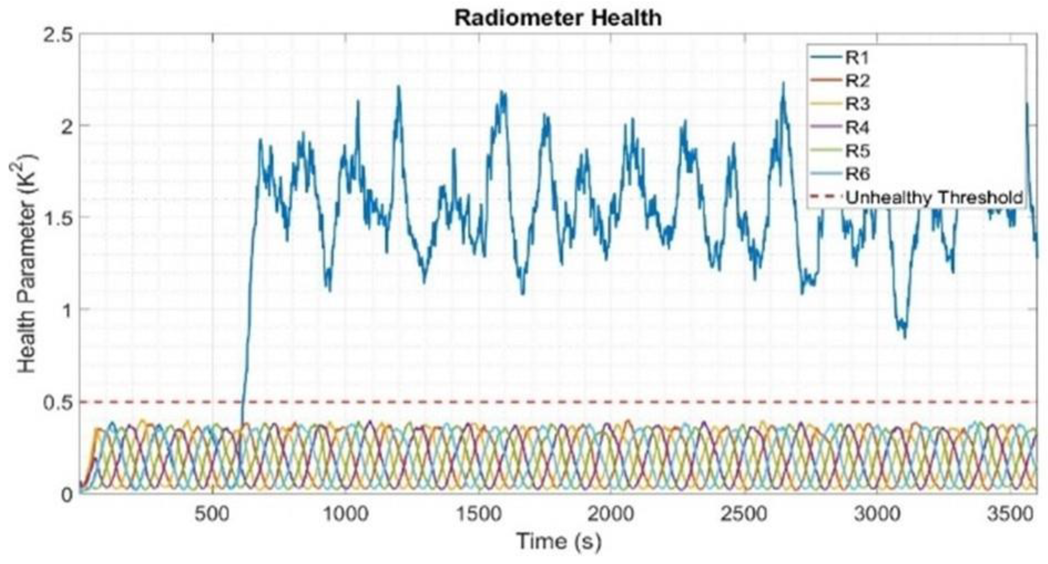
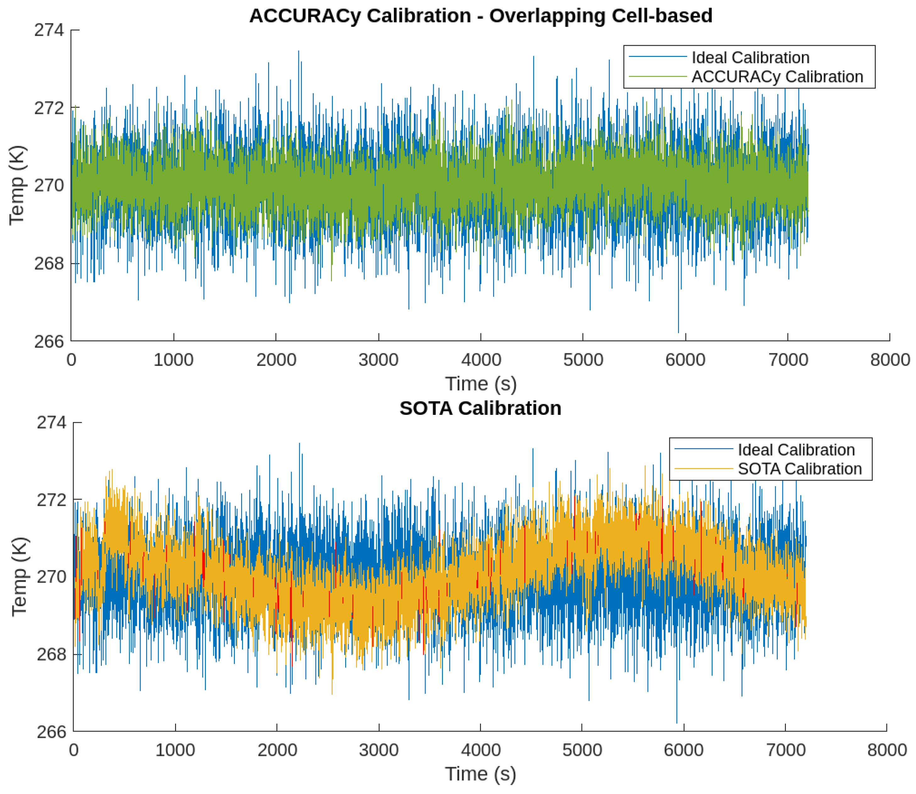
4.3. Simulation Results

ACCURACy is evaluated in terms of both calibration accuracy and ability to calibrate in real-time relative to the aforementioned post-processing SOTA intercalibration methods. In addition, an “ideal” intercalibration method, where every radiometer measurement can be calibrated using instantaneous two calibration measurements, is introduced to evaluate the improvement due to the additional volume of calibration data points made available by ACCURACy with its calibration pool module.

The total number of calibration measurements, which are collected by the constellation in SOTA algorithms, is determined by identifying, in a real-time simulation, when two instruments pass over the same location at nearly the same time. This is defined as when two instruments pass over the same one-degree cell of the Earth’s surface, within a specified interval T defined as T = 60 s. So, a change in the amount of calibration data collected within a time window can be determined between using ACCURACy and the SOTA methods. Additionally, the number of calibration measurements for a single radiometer can be tracked throughout the course of the simulation. This can be used to determine the number of times an instrument can be calibrated within a period of time, and the average time between calibrating.

One hundred constellation simulations were run for two hours using the parameters given in Table 2, Table 3 and Table 4, and

Table 5. RMSE and variance in the simulated calibrated antenna measurements.

Algorithm	RMSE (K)	${\mathit{\sigma }}^2$
Ideal	0.12	0.94
ACCURACy	0.16	0.60
SOTA	0.62	0.58

shows the root mean square error (RMSE) and the variance (${\sigma }^2$) of the estimated antenna temperature for the ideal calibration method, ACCURACy, and traditional SOTA algorithms obtained from one hundred simulation runs.

RMSE values given in Table 5 were calculated using the moving means of the calibrated antenna temperatures over 1 min windows, where each window has approximately 15,000 measurements, and the variance values are the average of variances calculated within the same windows throughout the simulation. The simulation results demonstrate that ACCURACy is able to provide accuracy as good as ideal calibration, and the uncertainty in the antenna temperatures calibrated by ACCURACy is as low as that resulted from the traditional SOTA methods. Note that the radiometer receiver noise temperature, integration time, and the bandwidth given in Table 4 lead to a variance of 0.34 K² as radiometric resolution, and the increases in variance values on top of the radiometric resolution are due to the uncertainties associated with calibration procedures as analytically described in Equations (12)–(14). ACCURACy and SOTA methods, due to the abundance of calibration measurements, cause smaller uncertainties compared to the ideal calibration where each radiometer is calibrated with its own calibration measurements only. On the other hand, the accuracy of the SOTA method suffers from the time difference between different calibration measurements where the radiometer gain characteristics do change. Such drifts cause systematic errors in the calibration defined by Equation (11), as the relationship between the voltage and temperature terms in the equation are different in antenna and calibration measurements performed at different times.

5. Discussion

The simulation produced calibrated measurements in real-time using ACCURACy, the conventional SOTA intercalibration methods, and a theoretical ideal calibration, resulting from a two-point calibration performed at every observation, using a 1 s integration time. This is termed “ideal” because it assumes there is a vicarious calibration measurement made by each radiometer every second, and establishes a baseline calibration for comparison.

The “ideal” calibration is seen in Figure 9, which compares the calibration accuracy when using ACCURACy and the SOTA methods to the ideal calibration. The ACCURACy calibration is shown with the green trace (top), and the conventional SOTA intercalibration method is shown in orange, on the bottom. On the SOTA trace, where the trace is red, there is sufficient calibration data, i.e., the overlapping measurements as described in the previous section, available to calibrate during that second and where the trace is yellow/orange, there is an insufficient amount of calibration data available to re-calibrate, and the estimated antenna temperature is obtained from the most recent calibration data. As expected, due to the time gaps between the overlapping measurements, the SOTA intercalibration shows large errors because of infrequent calibration. This reveals that SOTA methods are not suitable for real-time onboard constellation-level calibration. On the other hand, ACCURACy shows a strong improvement over the SOTA intercalibration in the simulation, as the calibration data sharing, facilitated by the calibration pool module, is independent of the time and location of the radiometer measurements. As long as the radiometers are in similar states, their calibration data become available to one another, which increases the amount of calibration data available to any constellation member at any time.

Figure 10 shows the calibration uncertainties and the moving mean for each of the ideal, SOTA, and ACCURACy calibration methods, calculated along a 1 min moving window. ACCURACy and the SOTA produce a very similar uncertainty in the estimated antenna temperatures, as they possess a large number of calibration data from multiple radiometers, unlike the ideal calibration, which is an individual radiometer calibration with two reference measurements, but the SOTA method lacks accuracy due to the infrequent collection of those calibration measurements.

Looking at the changes in the volume of calibration data and the ability to calibrate in real-time, Figure 11 illustrates the differences between ACCURACy and the SOTA intercalibration in terms of the volume and location of the calibration data, collected by a single constellation member and used in the calibration process. The SOTA method is not meant for real-time calibration, so this difference in performance is expected. The increase in the calibration data and time, where the calibration data are available are obvious. Further analyses may be conducted to determine the optimal calibration measurements in real-time, which also benefits from a greater pool of calibration data.

Currently, ACCURACy has been developed into a working prototype as a collection of MATLAB scripts, functioning with synthetic radiometer data, so there is a need to test and further improve ACCURACy using real data. The first planned collaboration is with MIT Lincoln Laboratory, using the TROPICS calibration data [28,29,39,40]. Analyzing TROPICS pre- and post-launch calibration data will also be useful to realistically model the relationship between the telemetry data and the radiometer gain characteristics, as well as the differences between “identical” CubeSat radiometers, and help to generalize ACCURACy by forming a methodology for the characterization of the radiometer gain for arbitrary CubeSat constellations. Other tasks include further use of IceCube data, specifically post-launch data, to analyze the changes in radiometer characteristics in space over time, studying the flow of errors and uncertainties from one ACCURACy module to another, and characterizing the relationship between adjustable parameters, calibration accuracy, and uncertainty requirements. Finally, hardware and data processing requirements for a successful real-time implementation of ACCURACy in actual CubeSat radiometers, communication needs between the constellation members to realize that the calibration data pool module in a real scenario, and the scalability of the ACCURACy framework for very large and very small constellations need to be studied. The authors plan to undertake those research tasks in the following years, and the results will be presented in future journal and conference papers, as ACCURAcy will be developed further into a mature intercalibration mechanism for CubeSat radiometer constellations observing Earth and planetary targets.

References

1. Brown, S.T.; Ruf, C.S. Determination of an amazon hot reference target for the on-orbit calibration of microwave radiometers. J. Atmos. Ocean. Technol. 2005, 22, 1340–1352. [Google Scholar] [CrossRef]
2. Wilheit, T. A model for the microwave emissivity of the ocean’s surface as a function of wind speed. IEEE Trans. Geosci. Electron. 1979, 17, 244–249. [Google Scholar] [CrossRef]
3. Elsaesser, G.S.; Kummerow, C.D. Toward a fully parametric retrieval of the nonraining parameters over the global oceans. J. Appl. Metereol. Climatol. JAMC 2008, 47, 1599–1618. [Google Scholar] [CrossRef]
4. Zou, C.; Goldberg, M.; Cheng, Z.; Grody, N.; Sullivan, J.; Cao, C.; Tarpley, D. Recalibration of microwave sounding unit for climate studies using simultaneous nadir overpasses. J. Geophys. Res. 2006, 111. [Google Scholar] [CrossRef]
5. Berg, W.; Bilanow, S.; Chen, R.; Datta, S.; Draper, D.; Ebrahimi, H.; Farrar, S.; Jones, W.L.; Kroodsma, R.; McKague, D.; et al. Intercalibration of the GPM microwave radiometer constellation. J. Atmos. Ocean. Technol. 2016, 33, 2639–2654. [Google Scholar] [CrossRef]
6. Chander, G.; Hewison, T.J.; Fox, N.; Wu, X.; Xiong, X.; Blackwell, W.J. Overview of intercalibration of satellite instruments. IEEE Trans. Geosci. Remote Sens. 2013, 51, 1056–1080. [Google Scholar] [CrossRef]
7. Selva, D.; Krejci, D. A survey and assessment of the capabilities of Cubesats for Earth observation. Acta Astronaut. 2012, 74, 50–68. [Google Scholar] [CrossRef]
8. Houtz, D.A.; Walker, D.K. A finite element thermal simulation of a microwave blackbody calibration target. In Proceedings of the 2013 IEEE International Geoscience and Remote Sensing Symposium (IGARSS), Melbourne, VIC, Australia, 21–26 July 2013; pp. 394–397. [Google Scholar]
9. Bouwmeester, J.; Gill, E.; Speretta, S.; Uludag, S. A new approach on the physical architecture of CubeSats & PocketQubes. In Proceedings of the 15th Reinventing Space Conference, Glasgow, UK, 24–26 October 2017; pp. 24–26. [Google Scholar]
10. Marinan, A.D.; Cahoy, K.L.; Bishop, R.L.; Lui, S.S.; Bardeen, J.R.; Mulligan, T.; Blackwell, W.J.; Leslie, R.V.; Osaretin, I.A.; Shields, M. Assessment of radiometer calibration with GPS radio occultation for the MiRaTA CubeSat mission. IEEE J. Sel. Top. Appl. Earth Obs. Remote Sens. 2016, 9, 5703–5714. [Google Scholar] [CrossRef] [PubMed]
11. Brown, S.T.; Desai, S.; Lu, W.; Tanner, A. On the long-term stability of microwave radiometers using noise diodes for calibration. IEEE Trans. Geosci. Remote Sens. 2007, 45, 1908–1920. [Google Scholar] [CrossRef]
12. Aksoy, M.; Bradburn, J.W. Accuracy: Adaptive Calibration of Cubesat Radiometer Constellations. In Proceedings of the 2020 IEEE Geoscience and Remote Sensing Symposium (IGARSS), Online, 26 September–2 October 2020; pp. 6357–6360. [Google Scholar]
13. Bradburn, J.W.; Aksoy, M.; Ashley, H.R. ACCURACy: Adaptive Calibration of Cubesat Radiometer Constellations. In Proceedings of the 2021 The U.S. National Committee for URSI (USNC-URSI) National Radio Science Meeting, Online, 4–9 January 2021; pp. 96–97. [Google Scholar]
14. Bradburn, J.W.; Ashley, H.R.; Aksoy, M. Accuracy: A Novel Approach to Calibrate Cubesat Radiometer Constellations. In Proceedings of the 2021 IEEE Geoscience and Remote Sensing Symposium (IGARSS), Brussels, Belgium, 11–16 July 2021; pp. 996–999. [Google Scholar]
15. Bradburn, J.; Aksoy, M. ACCURACy: Adaptive Calibration of CubeSat Radiometer Constellations. In Proceedings of the 2022 The U.S. National Committee for URSI (USNC-URSI) National Radio Science Meeting, Boulder, CO, USA, 4–8 January 2022; pp. 26–27. [Google Scholar]
16. Aksoy, M.; Bradburn, J.W. A Novel Calibration Framework for Cubesat Radiometer Constellations. In Proceedings of the 2022 IEEE Geoscience and Remote Sensing Symposium (IGARSS), Kuala Lumpur, Malaysia, 17–22 July 2022; pp. 4292–4295. [Google Scholar]
17. Gong, J.; Wu, D.L.; Eriksson, P. The first global 883 GHz cloud ice survey: IceCube Level 1 data calibration, processing and analysis. Earth Syst. Sci. Data 2021, 13, 5369–5387. [Google Scholar] [CrossRef]
18. Hollinger, E.J. DMSP Special Sensor Microwave/Imager Calibration/Validation—Final Report; Naval Research Lab: Washington, DC, USA, 1991. [Google Scholar]
19. Hollinger, J.; Peirce, J.; Poe, G. Ssm/i instrument evaluation. IEEE Trans. Geosci. Remote Sens. 1990, 28, 781–790. [Google Scholar] [CrossRef]
20. Biswas, S.K.; Farrar, S.; Gopalan, K.; Santos-Garcia, A.; Jones, W.L.; Bilanow, S. Intercalibration of microwave radiometer brightness temperatures for the global precipitation measurement mission. IEEE Trans. Geosci. Remote Sens. 2013, 51, 1465–1477. [Google Scholar] [CrossRef]
21. Draper, D.; Newell, D. Global precipitation measurement (GPM) microwave imager (GMI) after four years on-orbit. In Proceedings of the 2018 15th Specialist Meeting on Microwave Radiometry and Remote Sensing of the Environment (MicroRad), Cambridge, MA, USA, 27–30 March 2018; pp. 1–4. [Google Scholar]
22. Yang, J.X.; Mckague, D.S.; Ruf, C.S. Identifying and resolving a calibration issue with gmi. In Proceedings of the 2015 IEEE Geoscience and Remote Sensing Symposium (IGARSS), Milan, Italy, 16–21 July 2015; pp. 4753–5750. [Google Scholar]
23. Wilheit, T.; Berg, W.; Ebrahimi, H.; Kroodsma, R.; Mckague, D.; Payne, V.; Wang, J. Intercalibrating the GPM constellation using the gpm microwave imager (GMI). In Proceedings of the IEEE International Symposium on Geoscience and Remote Sensing, Milan, Italy, 26–31 July 2015; pp. 5162–5165. [Google Scholar]
24. Ebrahimi, H.; Datta, S.; Jones, W.L. Investigation of radiative transfer model effect on radiometric intercalibration of gpm sounder channels. In Proceedings of the 2015 IEEE Geoscience and Remote Sensing Symposium (IGARSS), Milan, Italy, 13–18 July 2015. [Google Scholar]
25. Draper, D.; Newell, D. Global precipitation measurement (GPM) microwave imager (GMI) calibration features and predicted performance. In Proceedings of the 2010 11th Specialist Meeting on Microwave Radiometry and Remote Sensing of the Environment (MicroRad), Washington, DC, USA, 1–4 March 2010; pp. 236–240. [Google Scholar]
26. Coakley, K.J.; Splett, J.; Walker, D.; Aksoy, M.; Racette, P. Microwave radiometer instability due to infrequent calibration. IEEE J. Sel. Top. Appl. Earth Obs. 2020, 13, 3281–3290. [Google Scholar] [CrossRef]
27. Wu, D.; Piepmeier, J.; Esper, J.; Ehsan, N.; Racette, P.; Johnson, T.; Abresch, B.S.; Bryerton, E. Icecube: Submm-Wave Technology Development for Future Science on a Cubesat; SPIE Digital Library: Bellingham, WA, USA, 2023. [Google Scholar] [CrossRef]
28. Blackwell, W.J.; Braun, S.; Bennartz, R.; Velden, C.; Demaria, M.; Atlas, R.; Dunion, J.; Marks, F.; Rogers, R.; Annane, B.; et al. An overview of the tropics NASA earth venture mission. Q. J. R. Meteorol. Soc. 2018, 144, 16–26. [Google Scholar] [CrossRef] [PubMed]
29. Blackwell, W.J. The NASA tropics mission as a pathfinder for future operational earth observing systems. In Proceedings of the 2020 IEEE Geoscience and Remote Sensing Symposium (IGARSS), Virtual Symposium, 26 September–2 October 2020; pp. 3647–3648. [Google Scholar]
30. Artac, M.; Jogan, M.; Leonardis, A. Incremental PCA for on-line visual learning and recognition. In Proceedings of the 2002 International Conference on Pattern Recognition, Quebec City, QC, Canada, 11–15 August 2002; Volume 3, pp. 781–784. [Google Scholar]
31. Khan, K.; Rehman, S.U.; Aziz, K.; Fong, S.; Sarasvady, S. DBSCAN: Past, present and future. In Proceedings of the Fifth International Conference on the Applications of Digital Information and Web Technologies (ICADIWT 2014), Chennai, India, 17–19 February 2014; pp. 232–238. [Google Scholar]
32. Chakraborty, S.; Nagwani, N.K. Analysis and Study of Incremental DBSCAN Clustering Algorithm. arXiv 2014, arXiv:1406.4754v1. Available online: http://arxiv.org/abs/1406.4754 (accessed on 15 May 2020).
33. Azhir, E.; Navimipour, N.J.; Hosseinzadeh, M.; Sharifi, A.; Darwesh, A. An efficient automated incremental density-based algorithm for clustering and classification. Future Gener. Comput. Syst. 2021, 114, 665–678. [Google Scholar] [CrossRef]
34. Singh, A.; Yadav, A.; Rana, A. Article: K-means with three different distance metrics. Int. J. Comput. Appl. 2013, 67, 13–17. [Google Scholar]
35. Racette, P.; Lang, R.H. Radiometer design analysis based upon measurement uncertainty. Radio Sci. 2005, 40, 1–22. [Google Scholar] [CrossRef]
36. Aksoy, M.; Rajabi, H.; Racette, P.E.; Bradburn, J. Analysis of nonstationary radiometer gain using ensemble detection. IEEE J. Sel. Top. Appl. Earth Obs. 2020, 13, 2807–2818. [Google Scholar] [CrossRef] [PubMed]
37. Aksoy, M.; Racette, P.E.; Bradburn, J.W. Analysis of non-stationary radiometer gain via ensemble detection. In Proceedings of the 2020 IEEE Geoscience and Remote Sensing Symposium (IGARSS), Yokohama, Japan, 28 July–2 October 2019; pp. 8893–8896. [Google Scholar]
38. Aksoy, M.; Racette, P.E. A preliminary study of three-point onboard external calibration for tracking radiometric stability and accuracy. Remote Sens. 2019, 11, 2790. [Google Scholar] [CrossRef]
39. Leslie, R.V.; Blackwell, W.J.; Cunningham, A.; Diliberto, M.; Eshbaugh, J.; Osaretin, I. Pre-launch calibration of the NASA tropics constellation mission. In Proceedings of the 2020 IEEE Geoscience and Remote Sensing Symposium (IGARSS), Virtual Symposium, 26 September–2 October 2020; pp. 1–4. [Google Scholar]
40. Surussavadee, C.; Blackwell, W.J.; Entekhabi, D.; Leslie, R.V. Precipitation retrieval accuracies of the tropics constellation of passive microwave cubesats. In Proceedings of the 2018 IEEE Geoscience and Remote Sensing Symposium (IGARSS), Valencia, Spain, 22–27 July 2018; pp. 3868–3871. [Google Scholar]
Figure 1. The ACCURACY monitoring panel showing relevant information as a set of synthetic radiometer data is processed in the calibration framework. (Top left) Measurements of a single thermistor from each radiometer shown in a different color, (top middle) current thermistor data for each constellation member shown in a different color, plotted post-principal component analysis (PCA) for clustering, (top right) a table tracking cluster labels and the number of calibration measurements available for each radiometer, (bottom left) gain plot of each radiometer shown in a different color, (bottom middle) plot showing the health of a single radiometer, defined as a measure of variance, (bottom right) health of each radiometer, shown in a different color, measured as the variance of thermistor measurements. Details about the framework parameters mentioned here are provided in Section 3.
Remotesensing 17 00486 g001
Figure 2. (Top) A diagram of the ACCURACy framework and its three modules. The figure is taken from [16]. (Bottom) Data pipeline of ACCURACy, with inputs and outputs shown at each step. Input calibration data and time are the raw input (1), which is preprocessed using PCA (2) before moving to the clustering Module (3). Class labels associated with the cluster for each radiometer are used to form/update calibration pools (4), which are then used for calibrating each radiometer (5). Details of data processing in ACCURACy modules are given in Section 3.1 and Section 3.2.
Remotesensing 17 00486 g002
Figure 3. The number of principal components determined from the percentage of explained variance. In this example 75% of the variance in the radiometer telemetry data can be explained by 3 principal components.
Remotesensing 17 00486 g003
Figure 4. The working principle of the overlapping cell-based clustering algorithm shown in a 2-D representation. The radiometer represented by Point A will give its calibration data to clusters 2, 3 and 4, since it falls within all three clusters. It will be calibrated using cluster 3, since it is the closest to its center. The radiometer represented by Point B, on the other hand, will only give its calibration data to cluster 2, and it will be calibrated using cluster 2.
Remotesensing 17 00486 g004
Figure 5. A total of 50 s of ACCURACy telemetry data plotted along three principal components, (Top Left) DBSCAN, (Top Right) IDBSCAN, (Bottom Left) Cell-based Clustering, (Bottom Right) Overlapping Cell-based Clustering. Large markers represent cluster centers and different colors indicate different clusters. Note the change in clustering for the same dataset when different clustering methods are applied. The overlapping cell-based clustering method outperforms the other algorithms.
Remotesensing 17 00486 g005
Figure 6. The “health” of each radiometer is tracked by ACCURACy, and if at any point a radiometer enters a failure state, it is removed from the calibration process. In this case, Radiometer 1 (R1) becomes unhealthy and is eliminated, i.e., its telemetry and calibration data are discarded in all ACCURACy modules.
Remotesensing 17 00486 g006
Figure 7. Synthetic data is generated using a set of models testing the ACCURACy framework. Starting with the orbital mechanics for each satellite, a time series of payload temperatures are generated for each satellite using modeled external and internal heat sources. These payload temperatures are used to generate the correlated telemetry data and instrument gains for all satellites in the constellation. Finally, instrument gains and offsets are used to process the calibration data to calibrate radiometer measurements.
Remotesensing 17 00486 g007
Figure 8. A simulation of 35 CubeSat radiometers orbiting Earth where each orbital plane is shown in a different color. Some of the CubeSats are on polar orbits, and some are orbiting close to tropical regions near the equator. This is in part to ensure there are sufficient opportunities for CubeSats to overlap in the simulation to compare ACCURACy with the SOTA algorithms.
Remotesensing 17 00486 g008
Figure 9. (Top) The calibration of one radiometer in the constellation using ACCURACy with an overlapping cell-based clustering algorithm (green), (Bottom) the calibration of the same radiometer using the SOTA calibration methods (yellow) with overlapping measurements (red). The algorithm requires some time before calibration is possible. The blue traces are the ideal calibration resulting from an assumption that frequent vicarious calibration measurements are made, and a two-point calibration is performed every second, with a 1 s integration time.
Remotesensing 17 00486 g009
Figure 10. (Left) The calculated uncertainty, i.e., the standard deviation of the calibrated antenna temperature over 1 min windows using the ideal (blue), SOTA (yellow), and ACCURACy (red) calibration methods. (Right) A moving mean of the calibrated antenna temperature calculated over a 1 min window for the ideal (blue), SOTA (yellow), and ACCURACy (red) methods where the true antenna temperature is 270 K, as shown in Table 4.
Remotesensing 17 00486 g010
Figure 11. After the full simulation (Top) using ACCURACy, one satellite maintains a high amount and frequency of calibration data to calibrate along its entire path thus far after four orbits. (Bottom) On the other hand, in the SOTA intercalibration, which is not ideal for real-time calibration, especially compared to ACCURACy, the entire constellation calibrates very infrequently during the same simulation.
Remotesensing 17 00486 g011