Beacon-Based Phased Array Antenna Calibration for Passive Radar

Abstract

Passive radar has drawn a lot of attention due to its applications across military and civilian sectors. Under this working paradigm, the utilization of antenna arrays is instrumental, as it increases the signal quality and enables precise target positioning. These promising features rely, however, on the precise calibration of the antenna array, as the different hardware components introduce impairments that compromise the beamforming capabilities of the system. We propose a technique that employs a low-power external beacon signal to produce precise information about the target location, avoiding the angular ambiguities present in other solutions in the literature. The experimental results demonstrate the method’s ability to effectively correct the amplitude and phase inconsistencies while compensating for frequency drifts, enabling beamforming capabilities and direction-of-arrival estimation. Among the tested beacon waveforms, the pseudo-random noise-based signals proved the most robust, especially in low-power scenarios. Additionally, the method was validated in a passive radar setup, where it successfully detected a vessel using opportunistic signals. These findings highlight the method’s potential to enhance passive radar performance while maintaining a low probability of detection, a key aspect in military applications, as well as its applicability to civilian purposes, such as infrastructure monitoring, environmental observation, and traffic management.

1. Introduction

Passive radar (PR) is a technology that has garnered significant attention within the military community since it allows for the detection of targets using signals emitted by other sources known as IoOs. That is, their working principle avoids the emission of any kind of signal [1,2]. In addition to its military applications [3,4,5], passive radar can also be utilized for civilian purposes [6], such as coherent change detection [7], displacement estimation [8], and traffic density monitoring [9], making it a versatile tool in various fields. In recent years, numerous PR systems have proven their capability utilizing signals from various types of IoOs, such as frequency modulation (FM) radio [10], digital video broadcasting–terrestrial (DVB-T) [11], digital audio broadcasting (DAB) [12], global system for mobile communications (GSM) [13], global navigation satellite system (GNSS) [14,15], and low-Earth orbit (LEO) communication satellites [16].

Accurately locating targets from the bistatic distances provided by PR systems, as well as the conversion of this data to Cartesian coordinates, requires estimating the direction of arrival (DoA) of the target echo signal. This can be achieved using an antenna array [17] by employing algorithms like multiple signal classification (MUSIC) [18]. It is well known that to perform an accurate DoA estimation, the received signal delays at each element of the antenna array must be coherent [19,20]. However, the different electronic components, such as the antenna elements themselves, connectors and cables, or the analog-to-digital converter (ADC), suffer from several impairments, such as meteorological conditions, aging effects [21], and mutual coupling between the antenna elements. Thereby, the performance of these elements will drift over time, resulting in arbitrary perturbations in both the amplitude and the phase of the different received signals [22,23]. These artifacts severely hinder the performance of the antenna array since the perturbation destroys the coherence among the antenna elements. Thus, the capability of discriminating signals by their spatial angles is no longer available, and it is impossible to steer the beam energy properly. In conclusion, a suitable calibration method must compensate for these drifts and achieve the theoretical performance granted by the antenna array [23].

A number of approaches were explored in previous studies to remove the amplitude and phase uncertainties. Mutual coupling between adjacent antenna elements can distort the antenna array radiation pattern and introduce DoA estimation errors. Compensation techniques for this scenario include estimating the calibration matrix between array elements and applying corrective measures using a decoupling matrix [24,25,26]. When a calibration technique is applied during the normal operation mode of the antenna array, it is not necessary to isolate the mutual coupling effects to estimate the uncertainties [27]. Indeed, all effects can be considered jointly, thus simplifying the calibration procedure. An alternative approach is to exploit an external source signal with known characteristics, such as carrier frequency and position, to calibrate the array antenna system. The received signal in each antenna array element is then compared with the known reference signal (generally, relative to one antenna array element), and adjustments are made to the antenna parameters to minimize any discrepancies according to the actual DoA. To this end, the direct path signal received from the illuminator of opportunity (IoO) itself, with a known position and frequency, has been commonly used as an external reference signal [28,29,30]. Recall, however, that the reference and surveillance signals should not interfere with each other, as their impact on the cross-ambiguity function (CAF) is strong and complicates the target detection. Accordingly, it is desirable to minimize the signal power of the reference signal contained in the surveillance signal using techniques like the extensive cancellation algorithm (ECA) [31,32]. Based on this, the IoO is often outside the boresight of the antenna array, so we might expect poor signal-to-noise ratio (SNR) levels and disturbances in the calibration procedure under this approach. Furthermore, mechanical steering of the antenna array to point at the IoO when a linear array is under use could lead to unexpected effects, invalidating the calibration procedure.

This work examined the calibration of ULAs for a PR system that leverages a signal transmitted from a known position that shares the carrier frequency with the IoO. We propose a two-stage method in which the frequency drift is first estimated and corrected, followed by the calibration of amplitude and phase uncertainties according to the initial correction. The whole procedure was designed to operate in real time during the passive detection stage and does not modify the operational mode of the PR system. Moreover, the radiation pattern of each antenna element is not required for the proposed method.

Although the beacon transmitter can be located in the neighborhood of the PR system, and the transmission power necessary to achieve the desired properties is minimal compared with that of the IoO, the beacon signal can be detected when the target of the PR is located in the vicinity of the beacon (i.e., in a range comparable with the distance between the PR and the beacon). In various applications, especially in defense, security, and advanced monitoring, the unlikely detection of the beacon signal might be unacceptable. The beacon’s emitted signals may inadvertently reveal the existence of a PR system undergoing calibration, potentially allowing adversaries to detect, locate, and classify it using signal intelligence (SIGINT) systems. To overcome this limitation, we propose the utilization of low-probability-of-intercept (LPI) signals during calibration so that the PR system can operate covertly, effectively concealing its location.

To achieve the desired capability of hiding the beacon signal, we propose the utilization of wideband code division multiple access (CDMA), a technique commonly used in other contexts to manage inter-user interference and/or prevent jamming. This technology assigns codes for transmission, which are known at both ends of the communication link, thus using a predefined sequence to encode the beacon signal. The receiver decodes the signal at the antenna array end to recover the original data [33]. A key feature is the utilization of codes such that their signal bandwidth is much larger than the one necessary for transmitting the beacon signal. As a consequence, the encoding process spreads the signal spectrum so that the transmitted beacon signal is no longer visible in the frequency domain, as it merges with the spectrum of the data signal of the IoO. That is, the beacon signal spectrum will remain unnoticeable. Besides the low probability of detection of the spread signal, using this scheme provides the additional benefit of reducing the chances of suffering jamming on the beacon signal since it is complicated to disturb a signal that is mixed with the one sent by the IoO.

We performed an extensive experiment campaign using the PR system located at the Defense University Center in the Spanish Naval Academy, where a DVB-T signal acted as the IoO. These experiments showed that the proposed method could calibrate the uniform linear array (ULA), and thus, provide spatial location capabilities to the PR system. We also showed this feature in a common PR scenario, where we detected and located a vessel that moved in the neighborhood of the PR systems.

Notation: Lower and upper case bold letters denote vectors, and ${\mathbb{C}}^M$ is a complex vector space with dimension M; ${\left(·\right)}^T$ and ${\left(·\right)}^H$ denote the transpose and Hermitian transpose operations, respectively; $\Re \{·\}$ and $\Im \{·\}$ represent the real and the imaginary parts of a complex number; the symbol ∼ reads as statistically distributed as and $E\left[·\right]$ is the statistical expectation; ${\mathcal{N}}_{\mathbb{C}}(\mathbf{0},\mathbf{C})$ is a zero-mean Gaussian distribution with covariance $\mathbf{C}$; $\parallel ·\parallel$ is the Euclidean norm; and ⊙ denotes the Hadamard product.

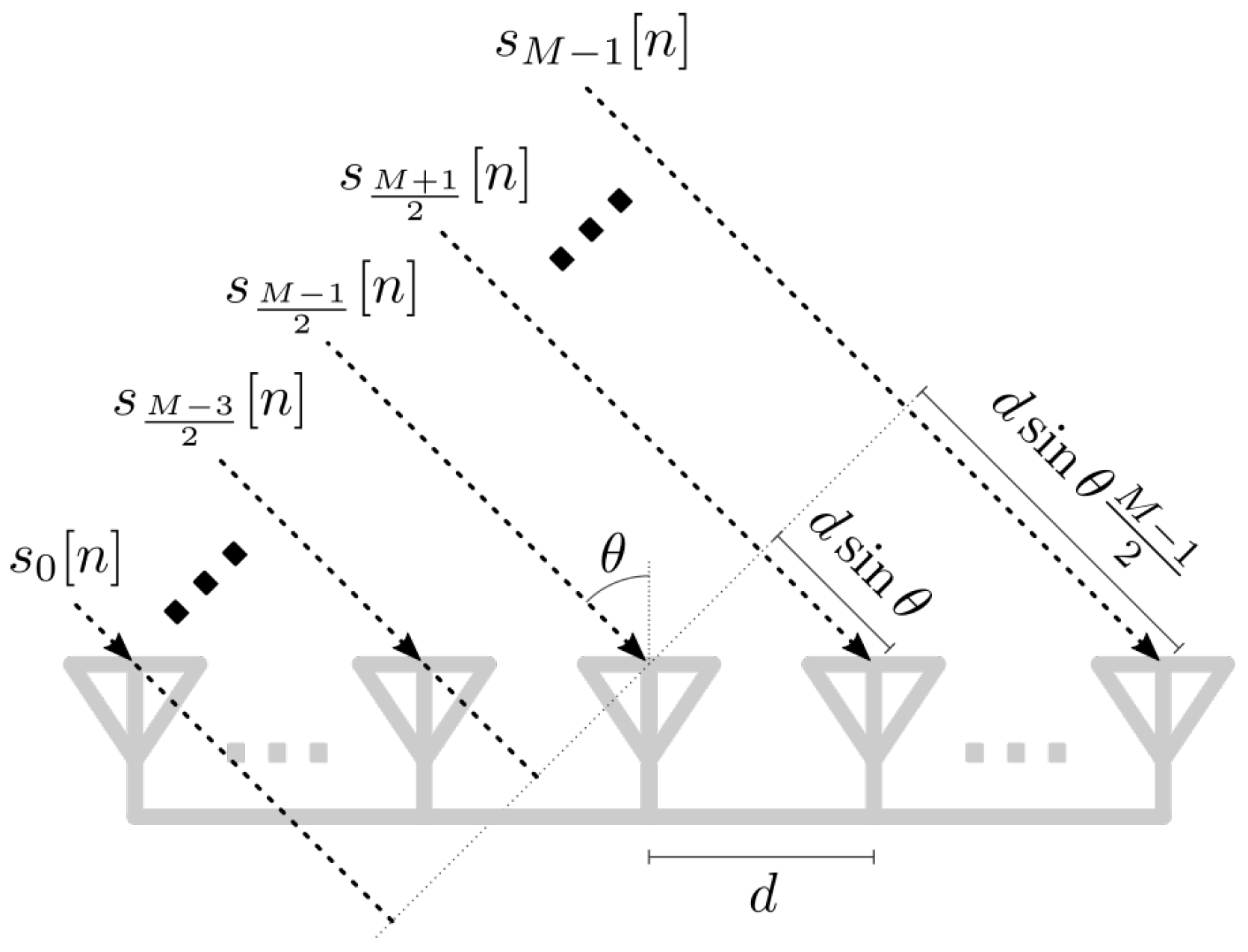
2. System Model

In this section, we describe the system of interest, where an antenna array equipped with M elements is sounding the environment to implement a PR system. We start by describing the transmitted signal, whose properties determine the mechanisms available at the receiver to compensate for the effects introduced by the hardware. In particular, we consider an RF signal at the transmitter $f\left(t\right)\in \mathbb{R}$, which is obtained from the complex baseband (IQ) source signal $x\left(t\right)$ in the following way:

$$f\left(t\right)=\Re \left\{x\left(t\right){\mathrm{e}}^{\mathrm{j}{\omega }_{c}t}\right\},$$

(1)

where ${\omega }_c=2\pi f_c$ is the carrier frequency (in rad/s). When we consider a general complex signal of the form $x\left(t\right)=a\left(t\right)+\mathrm{j}b\left(t\right)\in \mathbb{C}$, the RF signal decomposes as

$$f\left(t\right)=\Re \left\{x\left(t\right){\mathrm{e}}^{\mathrm{j}{\omega }_{c}t}\right\}=a\left(t\right)cos\left({\omega }_{c}t\right)-b\left(t\right)sin\left({\omega }_{c}t\right).$$

(2)

At the receiver side, and under ideal conditions (neglecting the effects of the noise, the channel, and other factors), the received signal is recovered by separating the IQ components and moving the signal back to the baseband frequency:

$$\begin{array}{cc}\hfill \Re \left\{2f\left(t\right){\mathrm{e}}^{-\mathrm{j}{\omega }_{c}t}\right\}& =a\left(t\right)+a\left(t\right)cos\left(2{\omega }_{c}t\right)-b\left(t\right)sin\left(2{\omega }_{c}t\right),\hfill \\ \hfill \Im \left\{2f\left(t\right){\mathrm{e}}^{-\mathrm{j}{\omega }_{c}t}\right\}& =b\left(t\right)-b\left(t\right)cos\left(2{\omega }_{c}t\right)+a\left(t\right)sin\left(2{\omega }_{c}t\right).\hfill \end{array}$$

Note from previous expressions that the IQ components, $a\left(t\right)$ and $b\left(t\right)$, of $x\left(t\right)$ can be recovered by using a low-pass filter for any practical signal bandwidth value of $x\left(t\right)$. In addition, prior to any digital processing, the received signal is sampled with an appropriate period $T_s=1/f_s$, leading to its discrete version $x\left[n\right]=x\left(n{T}_s\right)$. As the sampling periods in these systems are much shorter than the one required for acquiring $x\left(t\right)$, we consider the samples corresponding to the complex passband signal $s\left(t\right)=x\left(t\right){\mathrm{e}}^{\mathrm{j}{\omega }_{c}t}$ for the development of this work. In this way, the samples obtained depend not only on the frequency of the source signal but also on the variations experienced due to the carrier signal. In the following, we describe how this fact can be exploited if the receiver deploys multiple antenna elements.

Future radar systems, as well as wireless communication systems, will employ multiple antenna elements, as they enable achieving the so-called array gain and the exploitation of the spatial domain [34]. Thus, the receiver can acquire the signal from the multiple elements deployed in the array, and therefore, the received signal is a vector $\mathbf{s}\left(t\right)\in {\mathbb{C}}^M$ of dimension M that incorporates spatial information into the system. In particular, we consider that the geometric model of the array is that of the ULA in Figure 1. Moreover, we also consider the center of the array as a reference (i.e., the antenna element in the center is assumed to experience zero delay). Therefore, the delay experienced by the m-th element concerning the central one reads as

$${\tilde{\tau }}_m={\tau }_0+{\displaystyle \frac{dsin\left(\theta \right)\left(m-\frac{M-1}{2}\right)}{c}},m\in \left\{0,M-1\right\}$$

(3)

where d is the inter-element separation, c is the speed of light, and M is odd for the sake of notation simplicity. We denote as ${\tau }_0=r/c$ the delay for the central element, with r being the distance between the transmitter and the receiver. Note that ${\tilde{\tau }}_m<{\displaystyle \frac{dM}{2c}}$. According to Figure 1, each delay corresponds to that experienced by the wave that reaches each element, with a positive or negative sign, under the assumption of a plane wavefront and a line-of-sight (LoS) propagation model. This propagation model is reasonable for systems employing frequencies corresponding to the DVB-T and distances between the transmitter and the receiver that are much larger than the array size. Observe that all the parameters in (3) depend on the spatial configuration of the antenna array, i.e., they depend on the distance r and angle $\theta$, and that the travel time scales linearly with the index element m. This enables the receiver to perfectly locate the signal source using the associated polar coordinates.

Unfortunately, in practical scenarios, the delays do not obey (3). The underlying reasons for this fact are multiple and related to different effects introduced by hardware imperfections. For example, electronic components can drift over time with temperature and aging effects [21]; the cable lengths from antennas to ADCs could be slightly different; or there could be mutual coupling between antennas, especially when the spacing between the elements of the antenna array is less than $\lambda /2$ [35]. The different drifts will cause misinterpretations of the observed delays in (4), generally providing arbitrary values that lack coherence. As a consequence, these delays do not meet the expected values for the corresponding distance and angle and need to be compensated before fully exploiting the spatial and signal-enhancing capabilities provided by the antenna array. By taking into account the aforementioned effects, the arbitrary additional delay can be modeled as

$${\tau }_m={\tilde{\tau }}_m+{\tilde{\Delta }}_m.$$

(4)

Received Signal

In this section, we describe the features of the received signal, as the analysis of this signal is useful for compensating for the different drifts introduced by the hardware. Taking into account the procedure introduced to recover the source signal $x\left(t\right)$, and considering the aforementioned delays, the signal received at the m-th array element ${\left[\tilde{\mathbf{y}}\left(t\right)\right]}_m$ reads as

$$\begin{array}{cc}\hfill {\left[\tilde{\mathbf{y}}\left(t\right)\right]}_m& ={\phi }_m\beta x(t-{\tau }_m){\mathrm{e}}^{\mathrm{j}{\omega }_c(t-{\tau }_m)}+{\phi }_m{\left[\mathbf{z}\left(t\right)\right]}_m\hfill \\ \hfill & ={\phi }_m\beta x(t-{\tau }_m){\mathrm{e}}^{\mathrm{j}{\omega }_{c}t}{\mathrm{e}}^{-\mathrm{j}{\omega }_c{\tau }_m}+{\phi }_m{\left[\mathbf{z}\left(t\right)\right]}_m,\hfill \end{array}$$

(5)

where $\beta \in \mathbb{C}$ is the complex attenuation due to the propagation losses and other effects introduced by the wireless channel, ${\phi }_m\in \mathbb{R}$ corresponds to the attenuation suffered at the m-th antenna, and $\mathbf{z}\left(t\right)\in {\mathbb{C}}^M$ is the noise vector such that $\mathbf{z}\left[n\right]\sim {\mathcal{N}}_C(\mathbf{0},{\sigma }^2{\mathbf{I}}_M)$. At this point, it is also interesting to incorporate the variations introduced in the carrier frequency due to the lack of precision of the LOs, which are typically in the order of 10–100 parts per million with respect to the desired frequency ${\omega }_c$ [36]. These frequency variations are usually considered at the source signal and lead to a lack in the alignment of the signals received at the different antenna elements. It is thereby important to correct the carrier frequency deviation to detect and eliminate the phase offsets. By introducing the frequency drift $\varpi$, we obtain

$$\begin{array}{cc}\hfill {\left[\tilde{\mathbf{y}}\left(t\right)\right]}_m& ={\phi }_m\beta x(t-{\tau }_m){\mathrm{e}}^{\mathrm{j}({\omega }_c+\varpi )t}{\mathrm{e}}^{-\mathrm{j}({\omega }_c+\varpi ){\tau }_m}+{\phi }_m{\left[\mathbf{z}\left(t\right)\right]}_m.\hfill \end{array}$$

(6)

From our previous discussion, we aimed at recovering the baseband source signal by down-converting the received signal $\tilde{\mathbf{y}}\left(t\right)$, i.e., multiplying by the appropriate exponential function ${\mathrm{e}}^{-\mathrm{j}({\omega }_{c}t+\varphi )}$ provided by the local oscillator (LO). We consider that the LO is common to all the antenna elements so that the phase offset $\varphi$ is also shared among them [36]. Accordingly, the n-th sample of the baseband received signal for the m-th element is

$$\begin{array}{}\mathrm{(7)}& \hfill {\left[\mathbf{y}\left[n\right]\right]}_m& ={\left[\mathbf{y}\left(n{T}_s\right)\right]}_m={\phi }_m\beta x(n{T}_s-{\tau }_m){\mathrm{e}}^{-\mathrm{j}({\omega }_c+\varpi ){\tau }_m}{\mathrm{e}}^{-\mathrm{j}\varphi }{\mathrm{e}}^{\mathrm{j}\varpi n{T}_s}+{\phi }_m{\left[\mathbf{z}\left(n{T}_s\right))\right]}_m\hfill \mathrm{(8)}& & \approx {\phi }_m\beta x\left[n\right]{\mathrm{e}}^{-\mathrm{j}({\omega }_c+\varpi ){\tau }_m}{\mathrm{e}}^{-\mathrm{j}\varphi }{\mathrm{e}}^{\mathrm{j}\varpi n{T}_s}+{\phi }_m{\left[\mathbf{z}\left[n\right]\right]}_m\hfill \mathrm{(9)}& & ={\phi }_m\alpha x\left[n\right]{\mathrm{e}}^{-\mathrm{j}{\displaystyle \frac{{\omega }_c}{c}}dsin\left(\theta \right)\left(m-\frac{M-1}{2}\right)}{\mathrm{e}}^{\mathrm{j}{\Delta }_m}{\mathrm{e}}^{-\mathrm{j}\varphi }{\mathrm{e}}^{\mathrm{j}\varpi n{T}_s}+{\phi }_m{\left[\mathbf{z}\left[n\right]\right]}_m,\hfill \end{array}$$

where

$${\Delta }_m=-{\omega }_c{\tilde{\Delta }}_m-\varpi {\tau }_m,$$

(10)

$\alpha =\beta {\mathrm{e}}^{-\mathrm{j}{\omega }_c{\tau }_0}$ for notation simplicity, and the approach comes from considering the source signal that slowly varies in time when compared with the delays experienced by the different elements of the array. This a key assumption in the literature of array processing; see, e.g., [37]. In other words, the time delays are negligible when compared with the sampling period ${\tau }_m\ll T_s$, and the source signal $x\left(t\right)$ is assumed to be constant during such a short time interval. It is important to note that the frequency drift $\varpi$ produces a phase rotation that is different for each sample n. Consequently, we rewrite all the elements in vector notation as follows:

$$\mathbf{y}\left[n\right]=\alpha {\mathrm{e}}^{-\mathrm{j}\varphi }{\mathrm{e}}^{\mathrm{j}\varpi n{T}_s}x\left[n\right]\mathbf{a}\left(\theta \right)\odot \mathbf{d}+\mathbf{z}\left[n\right]\odot {[{\phi }_0,{\phi }_1,\dots ,{\phi }_{M-1}]}^T,$$

(11)

where we collect the theoretical and the phase shifts that depend on the antenna element m in the following vectors:

$$\begin{array}{}\mathrm{(12)}& \hfill \mathbf{a}\left(\theta \right)& ={\left[{\mathrm{e}}^{-\mathrm{j}{\displaystyle \frac{{\omega }_c}{c}}dsin\left(\theta \right){\displaystyle \frac{M-1}{2}}},{\mathrm{e}}^{-\mathrm{j}{\displaystyle \frac{{\omega }_c}{c}}dsin\left(\theta \right)\left({\displaystyle \frac{M-1}{2}}-1\right)},\dots ,{\mathrm{e}}^{\mathrm{j}{\displaystyle \frac{{\omega }_c}{c}}dsin\left(\theta \right){\displaystyle \frac{M-1}{2}}}\right]}^T,\hfill \mathrm{(13)}& \hfill \mathbf{d}& ={\left[{\phi }_0{\mathrm{e}}^{\mathrm{j}{\Delta }_0},{\phi }_1{\mathrm{e}}^{\mathrm{j}{\Delta }_1},\dots .{\phi }_{M-1}{\mathrm{e}}^{\mathrm{j}{\Delta }_{M-1}}\right]}^T,\hfill \end{array}$$

Note that in accordance with the time delay expression of (3), the vector $\mathbf{d}$ has, theoretically, unit amplitude and zero phase for each array element, that is, ${\phi }_m\approx 1$ and ${\Delta }_m=0$$\forall m$. However, both the amplitude and phase will differ from these theoretical values in practical scenarios. As an illustrative example, the antenna array pattern for the ideal vector $\mathbf{d}$ was compared with the simulated antenna array pattern when the amplitude and phase errors were introduced (Figure 2). As expected, small amplitude errors, about $\pm 25\%$ or less of the unit amplitude, led to a decrease in the sidelobe level (SLL) on the order of a couple of dB. This effect degraded the beamforming capabilities of the antenna array since it may not have been possible to combat the usual interferers in the PR scenarios, that is, the clutter signal and the direct path signal received from the IoO. Moreover, when the random amplitude errors were introduced, the nulls of the radiation pattern were much shallower than those of the theoretical pattern. In other words, the interference suppression capability of the antenna array dramatically decreased. Furthermore, adding phase errors at each element, with ${\Delta }_m\in \mathcal{N}(0,9)$$\forall m$, led to the antenna array pointing to a different angular direction, as the maximum was not achieved for ${20}^{\circ }$. In particular, the uncertainty vector $\mathbf{d}$ made the beamforming ineffective, as the arbitrary changes destroyed the relationship between the phases for the different antenna elements. Indeed, we obtained the maximum gain with a ${12}^{\circ }$ shift in the spatial angle.

Although both impairments were undesired, the theoretical amplitudes for all the antennas were the same, so this parameter did not provide any information regarding the position of the signal source. The phase caused by the imprecision of the LO was common to all the antennas and did not affect the determination of $\theta$. In contrast, the phase rotations that depended on $\varpi$ prevented the usage of the available samples, as this parameter was unknown and the rotation obeyed ${\mathrm{e}}^{\mathrm{j}\varpi n{T}_s}$. Based on these observations, we focused our efforts on correcting the estimation of the time delays ${\tau }_m$, $m\in \{0,\dots ,M-1\}$, to provide beamforming capabilities to the antenna array. Nevertheless, the amplitude correction could be achieved by simply scaling the signals for the different elements.

In the following section, we propose a procedure to compensate for the unknown arbitrary phase shifts contained in the vector $\mathbf{d}$.

3. Proposed Procedure

In the previous section, we present two different vectors containing the factors that affect each of the elements in the antenna array. While $\mathbf{a}\left(\theta \right)$ is fully determined by the angle $\theta$ of the transmitter with respect to the center of the antenna array, the carrier frequency, and the antenna array geometry, the factors $\mathbf{d}$, $\varphi$, and $\varpi$ are arbitrary and have to be estimated. To this end, we propose to employ a beacon located at a known position that sends a predefined signal within the spectrum of the signal of interest.

We consider the synchronization and the calibration procedures in the context of PR. As such, we focus on IoOs that are independent of the radar system and broadcast signals such as FM radio, DVB-T, or DAB. Therefore, as the spatial information contained in the vector $\mathbf{a}\left(\theta \right)$ depends on the carrier frequency ${\omega }_c$, we also need to adjust the beacon signal’s carrier frequency to that of the reference signal $r\left(t\right)=u\left(t\right){\mathrm{e}}^{\mathrm{j}{\omega }_{c}t}$, where $u\left(t\right)$ is the data signal sent by the IoO. In contrast, the correction applied to the vector coefficients would not be appropriate for the frequency band employed by the PR system.

To determine the waveform $g\left(t\right)$ contained in the beacon signal $b\left(t\right)=g\left(t\right){\mathrm{e}}^{\mathrm{j}{\omega }_{c}t}$, we have multiple candidates. However, it is desirable to select one of the kind that concentrates its power as a spike in the frequency domain, with the frequency value denoted by ${\omega }_0$, to identify and correct the frequency drift $\varpi$. Moreover, it will be easier to locate the beacon signal in the spectrum of the received signal, as detailed next. In particular, for a DVB-T channel, we select its central frequency ${\omega }_c$, and the frequency ${\omega }_0$ becomes a frequency shift with respect to the central channel frequency, with ${\omega }_0\ll {\omega }_c$ used to provide useful information regarding the phase shifts expected in the band of the reference DVB-T channel. At the receiver side, the samples in the discrete-time domain are given by

$$\begin{array}{}\mathrm{(14)}& \hfill b\left[n\right]& =g\left(n{T}_s\right){\mathrm{e}}^{\mathrm{j}({\omega }_c+{\omega }_0)n{T}_s},\hfill \mathrm{(15)}& \hfill r\left[n\right]& =u\left(n{T}_s\right){\mathrm{e}}^{\mathrm{j}{\omega }_{c}n{T}_s}\hfill \end{array}$$

as the unknown signal transmitted by the IoO $u\left(t\right)$ and the beacon waveform $g\left(t\right)$ are acquired at the same rate. At the receiver side, a linear combination of the beacon and the reference signal, together with the noise, is captured by each of the M elements deployed by the antenna array. That is, for the considered setup, the received signal for the n-th sample is given as follows:

$$\mathbf{y}\left[n\right]=\left({\alpha }_b{\mathrm{e}}^{-\mathrm{j}{\varphi }_b}{\mathrm{e}}^{\mathrm{j}{\varpi }_{b}n{T}_s}\mathbf{a}\left({\theta }_b\right)b\left[n\right]+{\alpha }_r{\mathrm{e}}^{-\mathrm{j}{\varphi }_r}{\mathrm{e}}^{\mathrm{j}{\varpi }_{r}n{T}_s}\mathbf{a}\left({\theta }_r\right)r\left[n\right]\right)\odot \mathbf{d}+\mathbf{z}\left[n\right]\odot {[{\phi }_0,{\phi }_1,\dots ,{\phi }_{M-1}]}^T,$$

(16)

where ${\alpha }_b$, ${\theta }_b$, ${\varphi }_b$, and ${\varpi }_b$ are the complex gain, spatial angle, phase offset, and frequency drift corresponding to the link between the beacon and the antenna array, and ${\alpha }_r$, ${\theta }_r$, ${\varphi }_r$, and ${\varpi }_r$ are those associated with the IoO. Note that for the sake of notation simplicity, we ignore the phase shifts over the noise, as they do not modify the properties of the noise covariance matrix. Moreover, both signals are affected by the Hadamard product times a common vector $\mathbf{d}$, as it depends on the mismatch effects introduced by the hardware at the receiver side. We take advantage of this feature to determine the spatial information of the reference signal by applying corrections based on the information provided by the beacon signal, for which the position is known. When a target is in the sounded area, delayed replicas of the reference signal arise, generally with gains lower than ${\alpha }_r$ and angles different from ${\theta }_r$. For the purpose of calibration, we neglect these signal components since identical conclusions to those for the reference signal apply. Following the procedure in (9), we develop the signal received by each element, which yields

$$\begin{array}{}\mathrm{(17)}& \hfill {\left[\mathbf{y}\left[n\right]\right]}_m& ={\alpha }_b{\phi }_m{\mathrm{e}}^{-\mathrm{j}{\varphi }_b}{\mathrm{e}}^{\mathrm{j}{\varpi }_{b}n{T}_s}g(n{T}_s-{\tau }_m){\mathrm{e}}^{-\mathrm{j}{\displaystyle \frac{{\omega }_c}{c}}dsin\left({\theta }_b\right)\left(m-\frac{M-1}{2}\right)}{\mathrm{e}}^{\mathrm{j}{\Delta }_m}\hfill \mathrm{(18)}& & +{\alpha }_r{\phi }_m{\mathrm{e}}^{-\mathrm{j}{\varphi }_r}{\mathrm{e}}^{\mathrm{j}{\varpi }_{r}n{T}_s}u(n{T}_s-{\tau }_m){\mathrm{e}}^{-\mathrm{j}{\displaystyle \frac{{\omega }_c}{c}}dsin\left({\theta }_r\right)\left(m-\frac{M-1}{2}\right)}{\mathrm{e}}^{\mathrm{j}{\Delta }_m}+{\phi }_m{\left[\mathbf{z}\left[n\right]\right]}_m\hfill & & \approx {\phi }_m\left({\alpha }_b{\mathrm{e}}^{-\mathrm{j}{\varphi }_b}{\mathrm{e}}^{\mathrm{j}{\varpi }_{b}n{T}_s}g\left(n{T}_s\right){\mathrm{e}}^{-\mathrm{j}{\displaystyle \frac{{\omega }_c}{c}}dsin\left({\theta }_b\right)\left(m-\frac{M-1}{2}\right)}\right.\hfill \mathrm{(19)}& & +\left.{\alpha }_r{\mathrm{e}}^{-\mathrm{j}{\varphi }_r}u\left(n{T}_s\right){\mathrm{e}}^{-\mathrm{j}{\displaystyle \frac{{\omega }_c}{c}}dsin\left({\theta }_r\right)\left(m-\frac{M-1}{2}\right)}\right){\mathrm{e}}^{\mathrm{j}{\Delta }_m}+{\phi }_m{\left[\mathbf{z}\left[n\right]\right]}_m.\hfill \end{array}$$

The frequencies for the IoOs, such as the DVB-T channels, are well known [38,39], and we consider that ${\varpi }_r=0$ in the last equation. The first step to approach the theoretical signal consists of the synchronization of the carrier frequencies to minimize or eliminate the frequency offset, i.e., the estimation of ${\varpi }_r$. To this end, we exploit the properties of the waveform $g\left(t\right)$ in the frequency domain, that is, the spectrum of $G\left[\omega \right]$ is very narrow and concentrates the signal power around the frequency shift ${\omega }_0$. By performing a search in the neighborhood of ${\omega }_0$, we try to determine the frequency deviation suffered by the beacon signal ${\varpi }_b$. Recall, however, that the beacon signal is located close to the center of the DVB-T channel, which might compromise the localization of the beacon signal, as the strategy consists of the localization of the frequency value showing a larger power, as we detail in Section 4. In the case of obtaining an accurate value, we can consider that the frequency drift is negligible, i.e., ${\varpi }_b\approx 0$.

Under the assumption of a correct synchronization procedure, we can safely process the available samples of the received signal to achieve a simpler representation in the frequency domain:

$$\begin{array}{}\mathrm{(20)}& \hfill {\left[\mathbf{Y}\left[\omega \right]\right]}_m& ={\phi }_m{\alpha }_b{\mathrm{e}}^{-\mathrm{j}{\varphi }_b}G\left[\omega \right]{\mathrm{e}}^{-\mathrm{j}{\displaystyle \frac{{\omega }_c}{c}}dsin\left({\theta }_b\right)\left(m-\frac{M-1}{2}\right)}{\mathrm{e}}^{\mathrm{j}{\Delta }_m}\hfill \mathrm{(21)}& & +{\phi }_m{\alpha }_r{\mathrm{e}}^{-\mathrm{j}{\varphi }_r}U\left[\omega \right]{\mathrm{e}}^{-\mathrm{j}{\displaystyle \frac{{\omega }_c}{c}}dsin\left({\theta }_r\right)\left(m-\frac{M-1}{2}\right)}{\mathrm{e}}^{\mathrm{j}{\Delta }_m}+{\phi }_m{\left[\mathbf{Z}\left[\omega \right]\right]}_m.\hfill \end{array}$$

Now, we can focus on the frequency sample corresponding to ${\omega }_0$, that is, the spike in the signal spectrum for the beacon waveform to obtain

$$\begin{array}{}& \hfill {\left[\mathbf{Y}\left[{\omega }_0\right]\right]}_m& ={\phi }_m\left({\alpha }_b{\mathrm{e}}^{-\mathrm{j}{\varphi }_b}G\left[{\omega }_0\right]{\mathrm{e}}^{-\mathrm{j}{\displaystyle \frac{{\omega }_c}{c}}dsin\left({\theta }_b\right)\left(m-\frac{M-1}{2}\right)}\right.\hfill \mathrm{(22)}& & +\left.{\alpha }_r{\mathrm{e}}^{-\mathrm{j}{\varphi }_r}U\left[{\omega }_0\right]{\mathrm{e}}^{-\mathrm{j}{\displaystyle \frac{{\omega }_c}{c}}dsin\left({\theta }_r\right)\left(m-\frac{M-1}{2}\right)}\right){\mathrm{e}}^{\mathrm{j}{\Delta }_m}+{\phi }_m{\left[\mathbf{Z}\left[{\omega }_0\right]\right]}_m\hfill \mathrm{(23)}& & \approx {\phi }_m{\alpha }_b{\mathrm{e}}^{-\mathrm{j}{\varphi }_b}G\left[{\omega }_0\right]{\mathrm{e}}^{-\mathrm{j}{\displaystyle \frac{{\omega }_c}{c}}dsin\left({\theta }_b\right)\left(m-\frac{M-1}{2}\right)}{\mathrm{e}}^{\mathrm{j}{\Delta }_m},\hfill \end{array}$$

where the last approach comes from assuming the signal power is larger than the reference signal and the noise, $|{\alpha }_{b}G\left[{\omega }_0\right]{|}^2>{\left|{\alpha }_{r}U\left[{\omega }_0\right]\right|}^2$, and $|{\alpha }_{b}G\left[{\omega }_0\right]{|}^2>{\left|{\left[Z\left[{\omega }_0\right]\right]}_m\right|}^2$. These inequalities are meaningful in the context of a beacon signal, where the source is located in the surroundings of the PR system, so we can expect $|{\alpha }_b|>|{\alpha }_r|$, and the beacon signal power is concentrated in a small portion of the spectrum, and thus, $|G\left[{\omega }_0\right]{|}^2>{\left|U\left[{\omega }_0\right]\right|}^2$. Based on the approach in (23), and taking into account the fact that the position of the beacon is known, ${\theta }_b$ and the corresponding signature of the beacon signal $\mathbf{a}\left({\theta }_b\right)$ are given. The approximated received signal vector in the frequency domain reads as

$$\begin{array}{}\mathrm{(24)}& \hfill \mathbf{Y}\left[{\omega }_0\right]& =\left({\alpha }_b{\mathrm{e}}^{-\mathrm{j}{\varphi }_b}G\left[{\omega }_0\right]\mathbf{a}\left({\theta }_b\right)+{\alpha }_r{\mathrm{e}}^{-\mathrm{j}{\varphi }_r}U\left[{\omega }_0\right]\mathbf{a}\left({\theta }_r\right)+\mathbf{Z}\left[{\omega }_0\right]\right)\odot \mathbf{d}\hfill \mathrm{(25)}& & \approx {\alpha }_b{\mathrm{e}}^{-\mathrm{j}{\varphi }_b}G\left[{\omega }_0\right]\mathbf{a}\left({\theta }_b\right)\odot \mathbf{d}.\hfill \end{array}$$

Note that for the purposes of beamforming or target detection required in PR systems, the phase and amplitude scalar variations of $\mathbf{Y}\left[{\omega }_0\right]$ in (24) are irrelevant, as we seek the ${\theta }_r$ value that maximizes

$${\widehat{\theta }}_r=\underset{\theta \ne {\theta }_b}{argmax}\sum _{\omega }|{\mathbf{a}}^H\left(\theta \right)\mathbf{Y}\left[\omega \right]|=\underset{\theta \ne {\theta }_b}{argmax}\sum _{\omega }U\left[\omega \right]|{\mathbf{a}}^H\left(\theta \right)(\mathbf{a}\left({\theta }_r\right)\odot \mathbf{d})\left)\right|,$$

(26)

to acquire spatial information about the scenario. Accordingly, the former problem leads to a meaningful ${\widehat{\theta }}_r$ value only if the effect of the drifts in $\mathbf{d}$ can be compensated. Therefore, we can safely scale the entries of the approach of $\mathbf{Y}\left[{\omega }_0\right]$ in (25) and gather the phases of such a vector to obtain an estimate of the drifts $\widehat{\mathbf{d}}$.

Finally, we simply perform the Hadamard product of the received signal times the complex conjugate $\mathbf{Y}\left[{\omega }_0\right]\odot \widehat{\mathbf{d}}$ to remove the phase shifts introduced by hardware imperfections. The resulting signal allows us to extract the spatial information of the other sources as follows:

$${\widehat{\theta }}_r=\underset{\theta \ne {\theta }_b}{argmax}\sum _{\omega }|{\mathbf{a}}^H\left(\theta \right)(\mathbf{Y}\left[\omega \right]\odot \widehat{\mathbf{d}})|\approx \underset{\theta \ne {\theta }_b}{argmax}\sum _{\omega }U\left[\omega \right]|{\mathbf{a}}^H\left(\theta \right)\mathbf{a}\left({\theta }_r\right)\left)\right|,$$

(27)

where the approximation comes from the estimation errors due to the noise and the other signal sources that interfere with the beacon signal.

Reducing the Probability of Detection

Thus far, we have introduced the working principles and the procedures that enable the correction of the frequency and phase drifts of the received signal. We have proposed to employ a beacon signal that is transmitted from a fixed position and that can be easily located in the spectrum of the received signal.

To grant LPI capabilities to the beacon signal, we employ a spreading code $c\left[n\right]$ known at both ends of the communication link. Then, the PR receiver computes a correlation of the received signal with $c\left[n\right]$ to recover the original signal from the source [33]. In particular, we rely on the pseudo-random noise (PRN) codes [40] for $c\left[n\right]$, which are often used in communications equipment, such as cellular telephones, or the global positioning system (GPS). This kind of sequence consists of a series of bits that lack any definite pattern and look statistically independent and uniformly distributed, exhibiting properties similar to noise. Moreover, these codes satisfy two requirements [40]: (I) There should be almost zero cross-correlation between the codes assigned to different transmitters; this does not apply to our case, as we only use a single beacon, but could be used to place additional beacons in scenarios that demand higher accuracy. (II) There must be zero correlation except for perfectly synchronized codes. This is important for guaranteeing that we can identify the frequency drift $\varpi$ without incurring ambiguities. The Gold codes proposed in [41] satisfy all these requirements.

4. Results

This section is devoted to the experimental evaluation of the proposed calibration method for the different beacon signals. We first describe the setup deployed to implement the PR system, and then we describe the experiments conducted to assess the benefits of the procedures described theoretically.

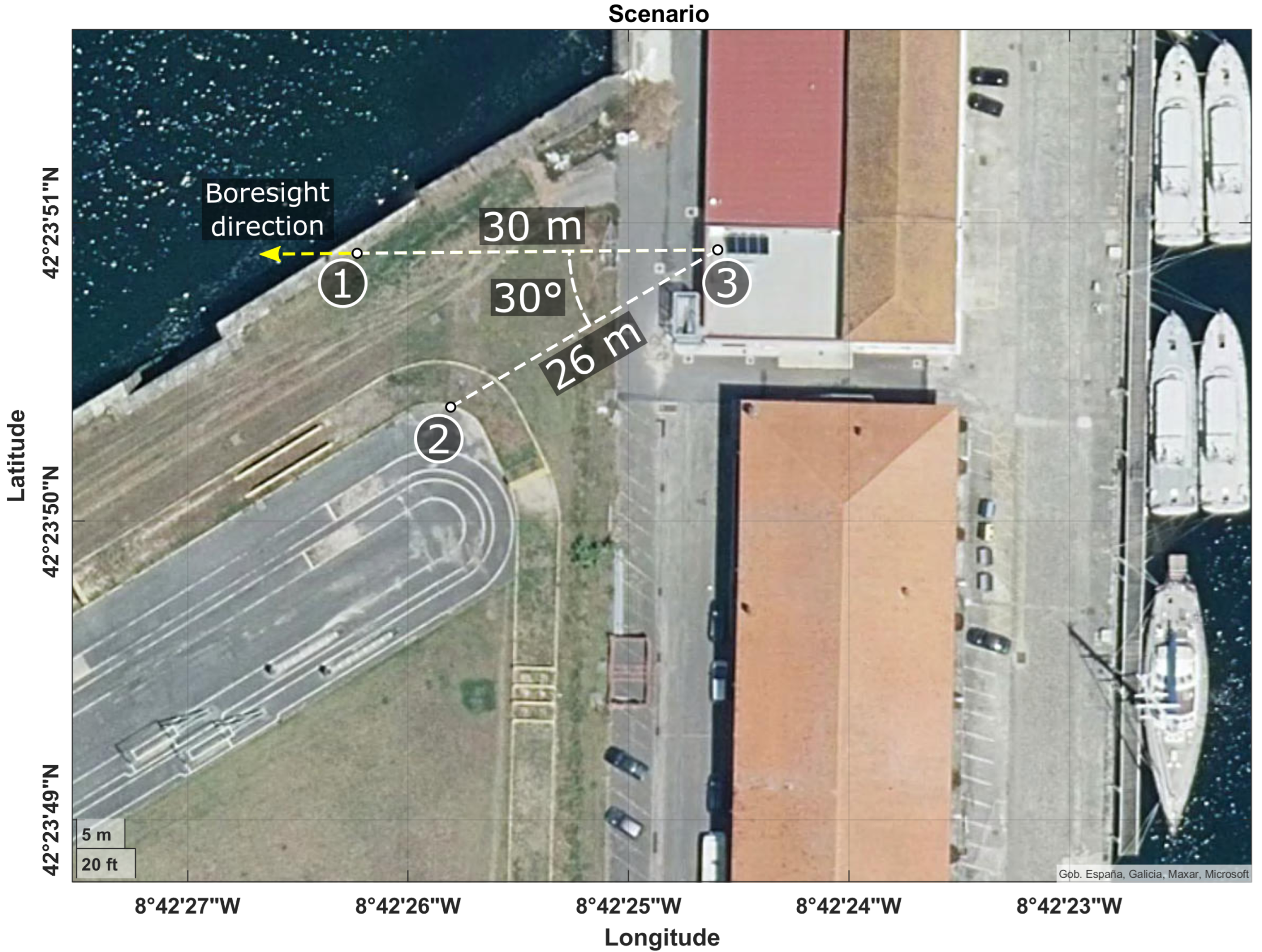
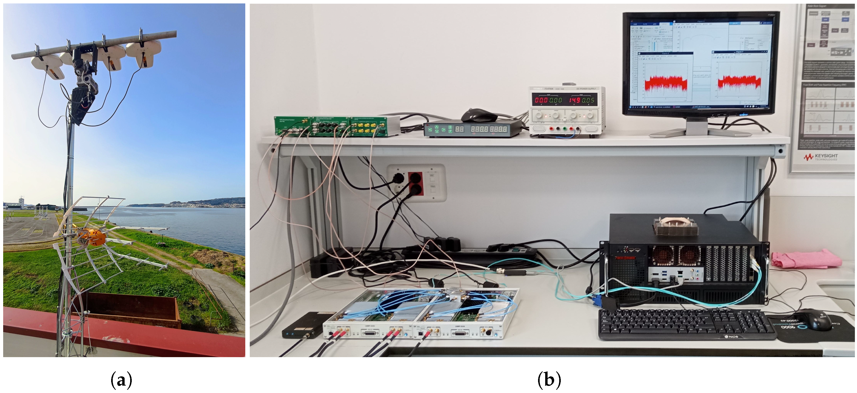
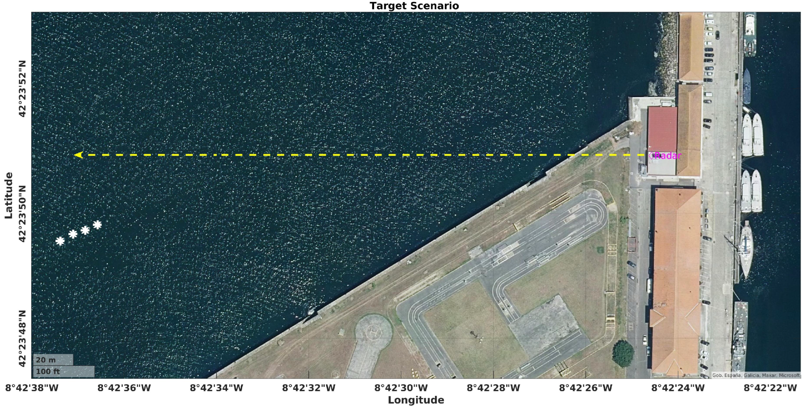
4.1. Scenario Description and Setup

The test scenario is located at the Defense University Center (CUD) at the Spanish Naval Academy in Marín, Pontevedra. A PR demonstrator based on DVB-T signals is available in the CUD research building. The locations of the different agents in the scenario are depicted in Figure 3: a beacon located at the boresight direction of the array antenna ➀, a simulated source ➁, and an antenna array ➂.

The antenna array, located at ➂ on the roof of the building, comprised four passive Televés Dinova Boss DVB-T antennas linearly arranged with a spacing of $d=\lambda /2$, as depicted in Figure 4a. The entire assembly is mounted on a rotor that during tests was always pointing 270° with respect to the north. The four antennas were directly connected to the inputs of an Ettus Research X310 Software-Defined Radio (SDR) receiver [42] (Figure 4b). This SDR was equipped with a pair of TwinRX cards that provided a total of four coherent sampling channels over a frequency range of 10–6000 MHz and with an instantaneous sampling bandwidth up to 80 MHz per channel. The sampling operations were synchronized with an external GPS disciplined oscillator (GPSDO) clock, with the SDR connected via a fiber optic link to a high-performance PC responsible for the sample storage and processing.

The beacon signal transmitter, located at ➀ in Figure 3, was based on a HackRF-One device, an SDR capable of transmitting low power radio signals from 1 MHz to 6 GHz [43]. The SDR was connected to a laptop from which the different types of beacon signals were parameterized and generated using the GNU Radio environment. The HackRF-One had a temperature-compensated crystal oscillator (TCXO) that generated the LO signal with a nominal frequency stability of ±20 parts per million, and produced a drift of up to 10 kHz in the DVB-T band, which made the estimation and correction of this frequency drift necessary.

Another HackRF-One device located at ➁ acted as a simulated source playing the role of a source of interest (an IoO, a target, etc.) and was used to validate the methods proposed in this paper.

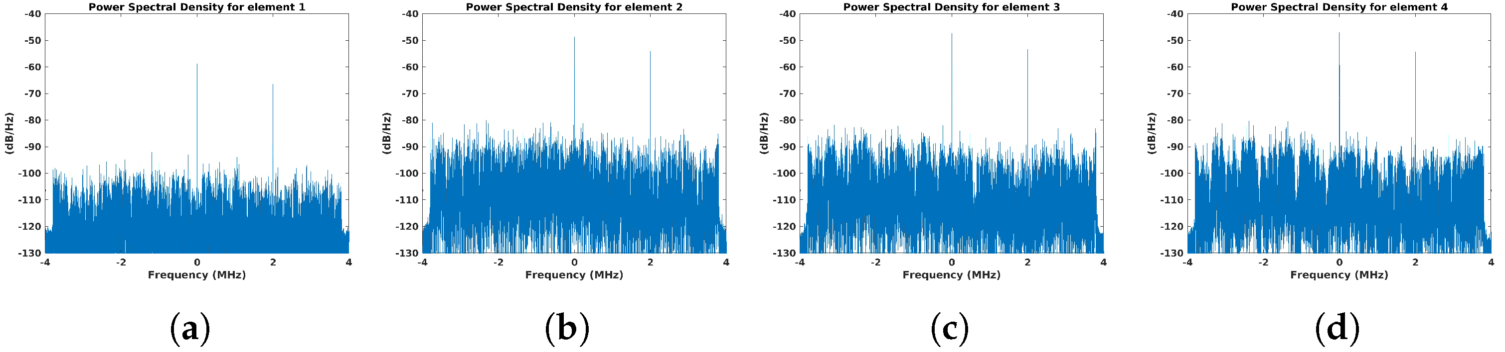
4.2. Beacon Signal Waveform

As mentioned in previous sections, to carry out the calibration procedure, it is necessary to both identify the frequency drift $\varpi$ and compensate for the effects of the drifts in each antenna array element collected in the vector $\mathbf{d}$. Both objectives can be accomplished using different waveforms $g\left(t\right)$ in the beacon signal. One option is to concentrate most of the beacon signal’s power at a single frequency within the DVB-T channel band, producing a spike in the spectrum. In this case, the waveform $g\left(t\right)$ can be a constant or a cosine signal. The other option is to spread the beacon signal spectrum along the DVB-T channel band using PRN codes. Below, the performance of each wavefront is then analyzed in depth.

In the following experiments, we evaluated the effect of the transmission power of the beacon over the power spectral density of the received signal. Figure 5 shows the received signal spectrum at one of the elements of the antenna array for the different beacon signal candidates. Moreover, it also shows the effect of using several gain values at the transmitter. We can see that the power spectral density for each waveform varied approximately between 5 dB and 40 dB, which corresponded precisely to the gain difference applied at the transmission. To correctly display the spectrum of each beacon signal, avoiding the presence of the reference signal $r\left(t\right)$ transmitted by the IoO, we used a free DVB-T transmission channel (between 486 MHz and 494 MHz). Later results in this section show that the power spectral density levels for the constant and cosine waveform candidates clearly exceeded the power spectral density for the DVB-T channel. In contrast, the PRN-based beacon waveform merged when both the beacon signal and the DVB-T transmission channel shared the same frequency band.

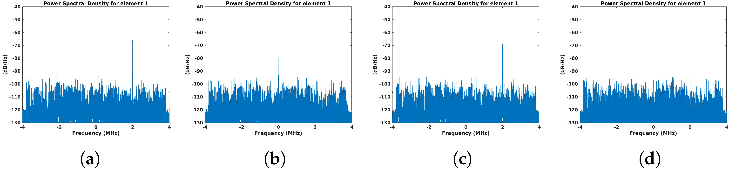
4.2.1. Constant Beacon Waveform

The simplest candidate waveform relies on concentrating the power of the beacon signal in a single frequency peak by modulating the carrier signal with a constant waveform, i.e., using $g\left(t\right)=k$, with k being a constant value. Under our scenario of application, the carrier frequency was set to 498 MHz, which was precisely the center of the DVB-T channel band. Accordingly, we expected to find a spike around such a frequency in the spectrum of the received signal. In addition, we also located an additional transmission source to validate the accuracy and convenience of the proposed procedure over a controlled signal source.

The power spectral density of the received signal is shown in Figure 6. For this experiment, we depicted the signal spectrum for each of the $M=4$ array elements. The gain at the beacon was set to 40 dB. We could see that the center of the frequency band presented a noticeable spike over the DVB-T signal spectrum. This could be observed for all the array elements, and it was important to ensure that the calibration procedure proposed in Section 3 could be conducted. It is worth mentioning that the other strong peak in the figures, located approximately 2 MHz apart from the frequency band center (i.e., at a frequency of 500 MHz), corresponded to the simulated source previously mentioned. This allowed us to extract the spatial signature of this additional source using the posed approach and compare it with the expected values.

We conducted multiple measurements with varying transmission gains to determine the practical values that ensured that the beacon signal remained effective while using the lowest possible transmitted power. Figure 7 shows the power spectral density with the first element of the array as the reference. The gain of the beacon ranged from 5 dB to 40 dB, with the power peak at the center of the frequency no longer identifiable for the lowest value, as depicted in Figure 7d. The consequences of this situation are dramatic for the proposed calibration method, as the synchronization stage will likely provide an inaccurate estimate of the frequency drift $\varpi$, leading to unacceptable errors in the acquisition of the vector $\mathbf{d}$.

Once the frequency drift $\varpi$ was identified, the effects of the phase offsets ${\Delta }_m$ in each antenna array element could be compensated, and the spatial information of the second signal source could be accurately obtained. Figure 8 shows the beamforming gain for the signal of interest at the receiver. That is, we computed $|{\mathbf{a}}^H\left(\theta \right)\mathbf{Y}\left[\omega \right]|$ for $\omega ={\omega }_c+\varpi$ and different values of $\theta$. In addition, we compared different gain values of 5, 10, 20, and 40 dB. The estimated spatial angle ${\widehat{\theta }}_r$ of the transmitter with respect to the array broadside direction was the one that maximized the received power. We represent these values for each gain using asterisk marks. We could see that when the gain value at the transmitter was large enough (i.e., when the power spectral density of the beacon waveform was larger than that of the DVB-T signal), the DoA was perfectly estimated and corresponded with the position of the source of interest (about −30° with respect to the broadside direction). However, when the gain value at the transmitter was reduced (for example, a gain value of 5 dB), the detection of the spike in the received signal spectrum presented an insufficient accuracy. As a consequence, the frequency drift $\varpi$ was not identified and ${\widehat{\theta }}_r$ was incorrectly estimated. Under this condition, the phases that affected each of the antenna elements lacked coherence, and the relationship with the spatial location of the source was lost. Therefore, the spatial angular estimation had a fairly random behavior, as the receiver signal gain was close to 0 dB for a wide range of angular positions.

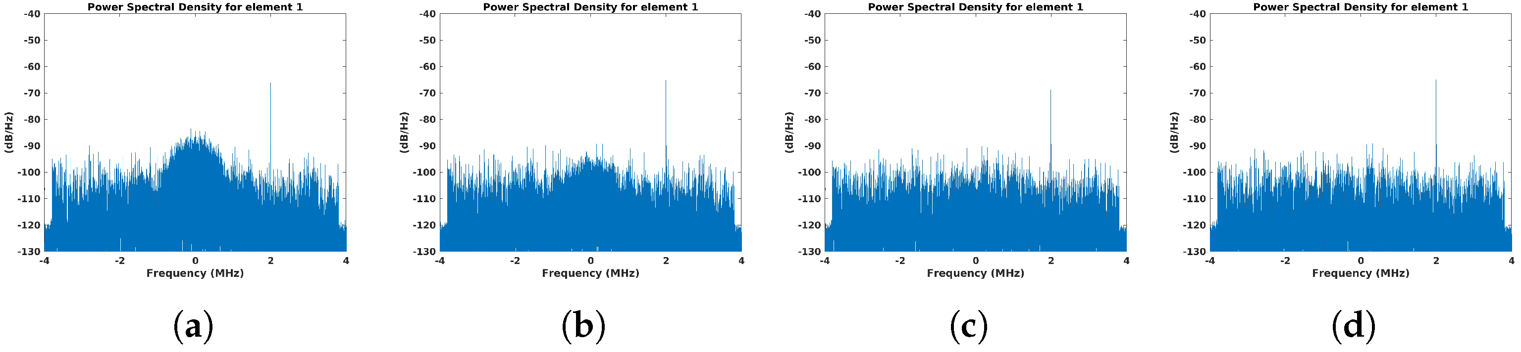
4.2.2. Cosine Beacon Waveform

The utilization of SDR provided the chance to employ alternative beacon waveforms. In particular, we modulated the carrier signal with a cosine waveform, that is, $g\left(t\right)=cos\left({\omega }_{0}t\right)$, where we kept the desired property of concentrating the beacon signal power on a single frequency peak. Furthermore, using a cosine waveform enabled a slight movement of this peak in the spectrum of the received signal. In this experiment, the carrier signal was set to ${\omega }_b=497.6$ MHz and was modulated by a cosine signal at 400 kHz, which resulted in the same modulated signal at 498 MHz as in the case of the constant beacon waveform. In fact, Figure 9 shows that the power spectral density of the received signal presented a high similarity to that shown in Figure 7 for gain values of the beacon from 5 dB to 40 dB. It should be noted though that in this case, the power peak at the center of the frequency band was no longer detectable, even for a gain of 10 dB. As a consequence, the frequency drift estimate and the acquisition of the vector $\mathbf{d}$ was not accurate.

Figure 10 shows the beamforming gain at the receiver for the signal of interest when the cosine beacon waveform was transmitted. The asterisk marks represent the spatial angle ${\widehat{\theta }}_r$ of the second transmitter with respect to the array broadside direction. As expected, when the power spectral density of the cosine beacon waveform was larger than that of the DVB-T signal, the pointing angle was perfectly estimated at approximately −30° with respect to the broadside direction. However, when the gain value at the transmitter was reduced to 5 dB or 10 dB, the detection of the spike on the received signal spectrum presented insufficient accuracy to identify the frequency drift, which spoiled the subsequent estimation of the spatial angle.

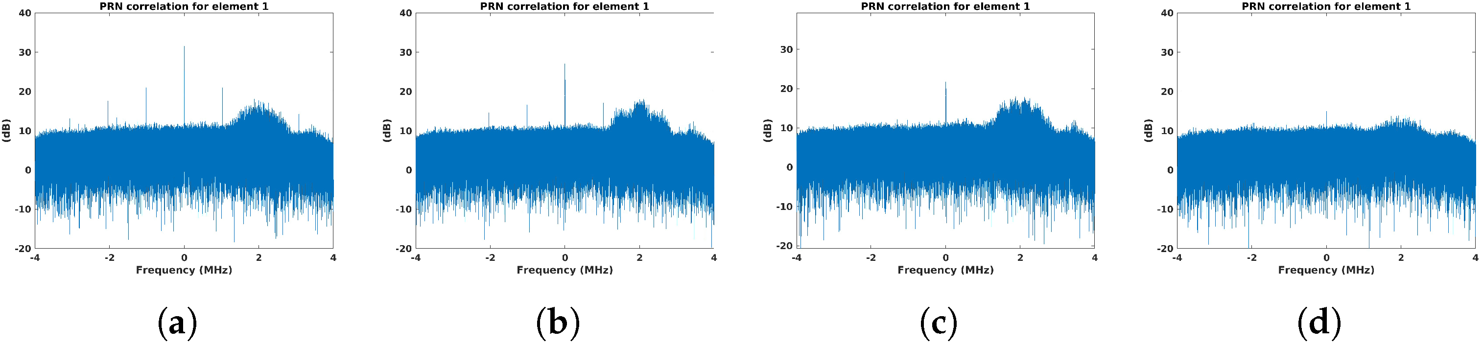
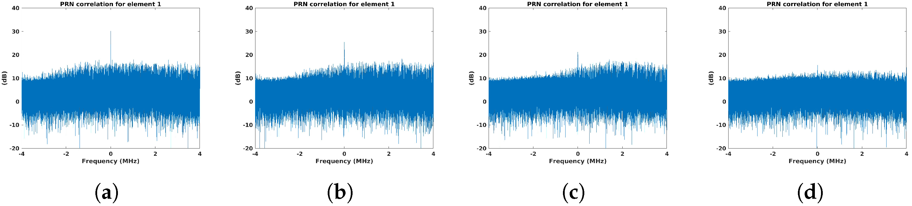
4.2.3. PRN-Based Beacon Waveform

As previously stated, in some scenarios where PR is meaningful, it may be of special interest that the spectrum of the beacon signal spreads over the IoO spectrum to achieve a low probability of detection in the calibration process. To achieve this interesting capability, in this experiment, a PRN code $c\left[n\right]$ of 1023 bits was transmitted during uninterrupted time periods of 1 ms while spreading its spectrum by approximately 1 MHz (see Figure 5c). The carrier frequency remained at the center of the DVB-T channel band (i.e., 498 MHz). The beacon signal therefore obeyed

$$b\left[n\right]=c\left[n\right]g\left(n{T}_s\right){\mathrm{e}}^{\mathrm{j}{\omega }_{c}n{T}_s}.$$

(28)

Depending on the gain value selected for the beacon, it might happen that the power spectral density of the PRN-based beacon waveform spread at 1 MHz was larger than the power spectral density of the IoO signal (for example, see Figure 11a,b for gain values of 40 dB and 30 dB, respectively). Accordingly, the beacon signal allows for an accurate antenna array calibration, but it can be detected for any receiver located at a position where the distance to the beacon and, consequently, the received beacon signal power, are similar to that of the antenna array. In contrast, if the gain selected for the beacon is reduced to 20 dB or 10 dB, the power spectral density of the PRN-based beacon waveform is completely merged with the power spectral density of the IoO signal, making it difficult to detect the beacon signal (see Figure 11c,d). Similar to the previous experiments, we kept the additional simulated source for the purpose of validating our method.

As a first step to identifying the frequency drift $\varpi$ and to estimate the vector $\mathbf{d}$, a correlation between the received signal and the spreading code was computed. We can see in Figure 12 that the correlation presented low values, except for the strong peak near the center of the frequency band, which allowed for identifying $\varpi$ accurately. As expected, the amplitude of the correlation peak decreased with diminishing gains at the beacon.

It is worth mentioning that the PRN code can be transmitted at a larger rate, broadening the beacon signal spectrum as much as possible within the available bandwidth for the DVB-T signal. In this mode, the 1023-bit PRN code was transmitted during time periods of 0.2 ms, which resulted in a spectrum spreading of about 5 MHz (see Figure 5d). Figure 13 depicts the power spectral density of the PRN-based beacon waveform spread at 5 MHz and the power spectral density of the IoO signal that modified the gain at the transmitter. In Figure 13a,b, the power spectral density of the PRN-based beacon waveform was larger than the power spectral density of the IoO signal for gain values at the transmitter of 40 dB and 30 dB, respectively. In contrast, in Figure 13c,d, the power spectral density of the PRN-based beacon waveform was lower than that of the IoO signal, and consequently, it remained unnoticeable. The signal spectrum at the receiver after performing the correlation with the spreading code is shown in Figure 14. Again, the respective frequency peaks located near the center of the frequency band could be perfectly identified.

Figure 15a,b show the beamforming gain at the receiver for the signal of interest when the PRN-based beacon waveform was transmitted at 1 MHz and 5 MHz, respectively. The asterisk marks represent the spatial angle ${\widehat{\theta }}_r$ of the second transmitter with respect to the array broadside direction. As expected, when the power spectral density of the PRN-based beacon waveform is larger than that of the DVB-T signal, ${\widehat{\theta }}_r$ is perfectly estimated at approximately −30° with respect to the broadside direction. However, unlike the constant and cosine beacon waveforms, when the gain value at the transmitter was reduced to merge the spectrum of the PRN-based beacon within the IoO spectrum, the detection of the spike on the correlation function still presented enough accuracy to identify the frequency drift and to estimate the spatial angle. When comparing the PRN-based beacon waveform with the constant and cosine waveforms, which concentrated the power in a frequency spike, the estimation of ${\widehat{\theta }}_r$ was more robust. Indeed, the accuracy of the angle estimation worsened gradually as the gain value at the transmitter decreased, i.e., as the noise power in the vector $\mathbf{d}$ increased. In contrast, the accuracy of the estimation decreased dramatically when a constant or a cosine beacon waveform was used, as the frequency drift was not detected correctly.

In summary, when the gain value applied at the beacon was large enough, the proposed method allowed for both the estimation of the frequency drift $\varpi$ and the compensation for the phase drift effects on each antenna element, which were collected in the vector $\mathbf{d}$. In this way, the estimation of the spatial angle ${\widehat{\theta }}_r$ of the simulated source was feasible. However, one key feature in a PR scenario is being unnoticeable. Based on this idea, it is interesting to measure the error in the estimation of the spatial angle ${\widehat{\theta }}_r$ by analyzing the power spectral densities of the beacon signal peak and the IoO signal since a beacon signal might remain unnoticed when the maximum of its power spectral density is lower than that of the DVB-T channel. Figure 16 shows the error in the calibration procedure calculated as the difference between the estimated spatial angle of (27) and the true spatial angle. We computed this error from a single measurement for each of the different beacon waveforms and transmission gains. It is important to note that the estimation accuracy depends on how prominently the beacon signals merge with or stand out from the spectrum of the IoO signals. We show that the beacon signals with peaks 20 dB higher than the IoO signal yielded negligible estimation errors for all the waveforms evaluated. When the power spectral density variation approached zero, the estimated spatial angle obtained with the constant and cosine waveforms became arbitrary, as the frequency drift was not correctly identified. Nevertheless, the accuracy obtained with the PRN-based waveform remained at acceptable values until there were power spectral density variations of about −10 dB. Furthermore, when the power spectral density variation was reduced below −10 dB, the estimation error increased smoothly compared with the abrupt growth of the other waveforms. The main reason was that even in such a challenging scenario, the frequency drift was identified thanks to the properties of the PRN-based waveform. The error then came from the lack of compensation for the phase drifts in the vector $\mathbf{d}$ due to the noise and interference levels present in the correlation procedure.

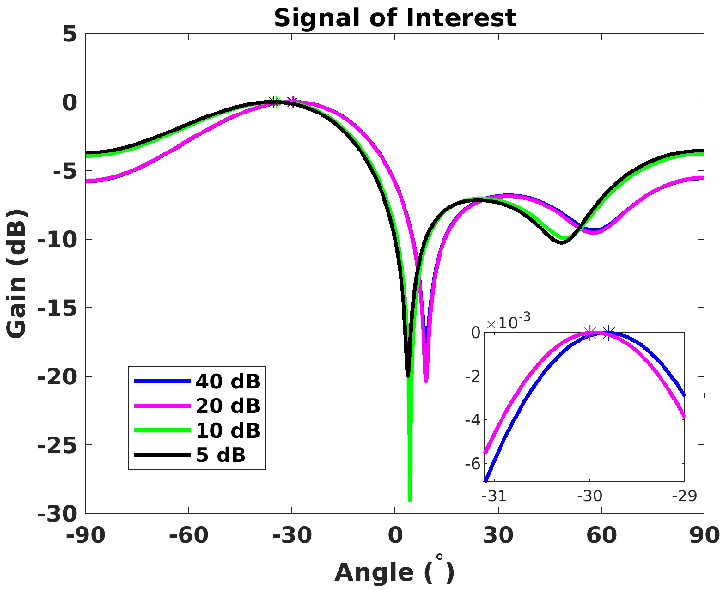
4.3. Robustness Against Location Errors

In this section, we discuss the robustness against subtle errors in the location errors of the beacon ➀ and an antenna array ➂ of the setup in Section 4.1. Since the ultimate goal of calibrating the antenna array was to grant spatial resolution capabilities to our system, we carried out our analysis from this perspective. First, we introduce the concept of a half-power beamwidth (HPBW), which is a measure of the width of the beam [37]. If the antenna array is pointing toward the spatial angle ${\theta }_t$, the HPBW is the range of spatial angles $\theta$ for which the product $|{\mathbf{a}}^H\left({\theta }_t\right)\mathbf{a}\left(\theta \right){|}^2\ge 0.5$. To be more precise, we considered the interval for which $|{\mathbf{a}}^H\left({\theta }_t\right)\mathbf{a}\left(\theta \right){|}^2\ge 0.9$, which made the response vectors (and also the associated spatial angles) hardly distinguishable under the limitations imposed by the spatial resolution provided by our antenna array. We compared the resulting distance with practical values for errors in the location of the agents in our setup. In particular, for the scenario of Section 4.1, this interval corresponded to ${\theta }_t\pm 5^{\circ }$. Taking into account the fact that the distance from the antenna array ➂ to the beacon transmitter ➀ was 30 m, the position error resulted in $ϵ=30tan\left(5^{\circ }\right)\approx 2.7$ m. Hence, we concluded that this error distance was huge compared with practical values for the considered setup below $0.5$ m, and therefore, the proposed method was robust against small position errors.

4.4. Passive Radar Detection System

The target detection in a PR scenario relies on a comparison between a direct signal coming from the IoO and an echo signal reflected by the target. In our case, the SDR receiver system could capture four different signals simultaneously. Therefore, one of these channels was used to capture the reference signal (the direct signal), and the three remaining channels were used to capture the surveillance signal (reflected signal). Thus, in this experiment, we considered a ULA receiver antenna composed of three antennas that were equally spaced with a distance $d=\lambda /2$ for a frequency of 498 MHz, which corresponded to a DVB-T channel. The reference channel was connected to a Televés Ellipse DVB-T antenna (Figure 4a) pointing at ${31}^{\circ }$ with respect to north, where the DVB-T transmitter of Tomba mountain is located, which covers the city of Pontevedra and its surroundings. This opportunistic waveform allowed for reaching a maximum range resolution of 18 m [34]. A coherent processing interval (CPI) of 1 s was selected in order to achieve a Doppler resolution below 1 Hz.

In the next example, a small vessel was detected within the PR coverage area when the beacon transmitted the PRN-based waveform at 5 MHz with a transmitter gain of 20 dB, i.e., when the power spectral density of the beacon was lower than the power spectral density of the IoO. Figure 17 shows the range–Doppler map derived from this detection after the ECA filter was applied. In particular, the small vessel was detected at a bistatic distance of approximately 240 m and moved toward the receiver at a Doppler velocity of roughly 12 Hz.

Once the array was calibrated and a constant false alarm rate (CFAR) algorithm was applied to the range–Doppler map, the estimation of the DoA angle for the detected targets within the area of interest could be carried out from the respective echo spatial responses. In particular, the DoA angle corresponded to the maximum value of each spatial response. Figure 18 shows the estimated DoA angle tracking for the small vessel and four consecutive CPIs, i.e., during 4 s. We can see that the DoA angle decreased from $-8.2^{\circ }$ to $-7.1^{\circ }$ as the target trajectory approached the broadside direction of the radar.

Finally, knowing the bistatic distance and the DoA angle, we could make a one-to-one transformation from a range–Doppler map to a Cartesian coordinates map, which is displayed in Figure 19 using white asterisks to represent the trajectory followed by the vessel during the tracking period. The broadside direction of the radar is also represented by a yellow dotted line in this figure.

5. Conclusions

In this paper, we present a novel calibration methodology for a phased antenna array that is deployed in a passive radar system and leverages beacon signals to address hardware-induced deviations. Our approach effectively compensates for amplitude and phase inconsistencies while simultaneously correcting frequency drifts. Therefore, it restores coherence among antenna elements enabling accurate beamforming. Compared with other methods available in the literature that employ an external or beacon signal for the calibration procedure, we propose employing constant or cosine beacon signals aligned with the antenna array’s boresight while ensuring the illuminator of opportunity remains outside the boresight direction. This approach is further enhanced by the application of post-calibration filtering techniques to preserve the CAF performance. Additionally, LPI signals, such as PRN-based beacons, offer a stealthy alternative by merging the beacon within the spectrum of the illuminator signal, ensuring accurate calibration while maintaining system discretion. The experimental evaluation revealed several critical insights:

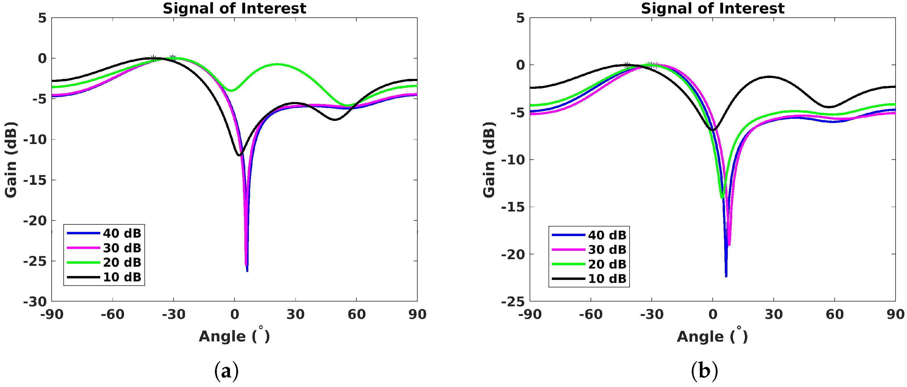
• Signal integrity: the proposed calibration procedure reliably identified and corrected frequency drifts and phase mismatches under various conditions, and thus, significantly enhanced the DoA estimation accuracy and ensured precise alignment of antenna elements.
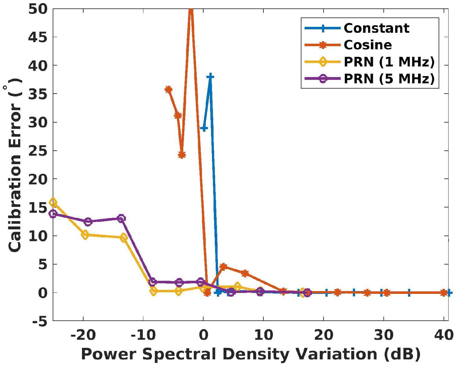
• Beacon waveform selection: among the tested waveforms, the PRN-based signal demonstrated superior robustness, particularly in challenging scenarios where the power spectral density of the IoO contribution was similar to or even larger than that of the beacon signal.
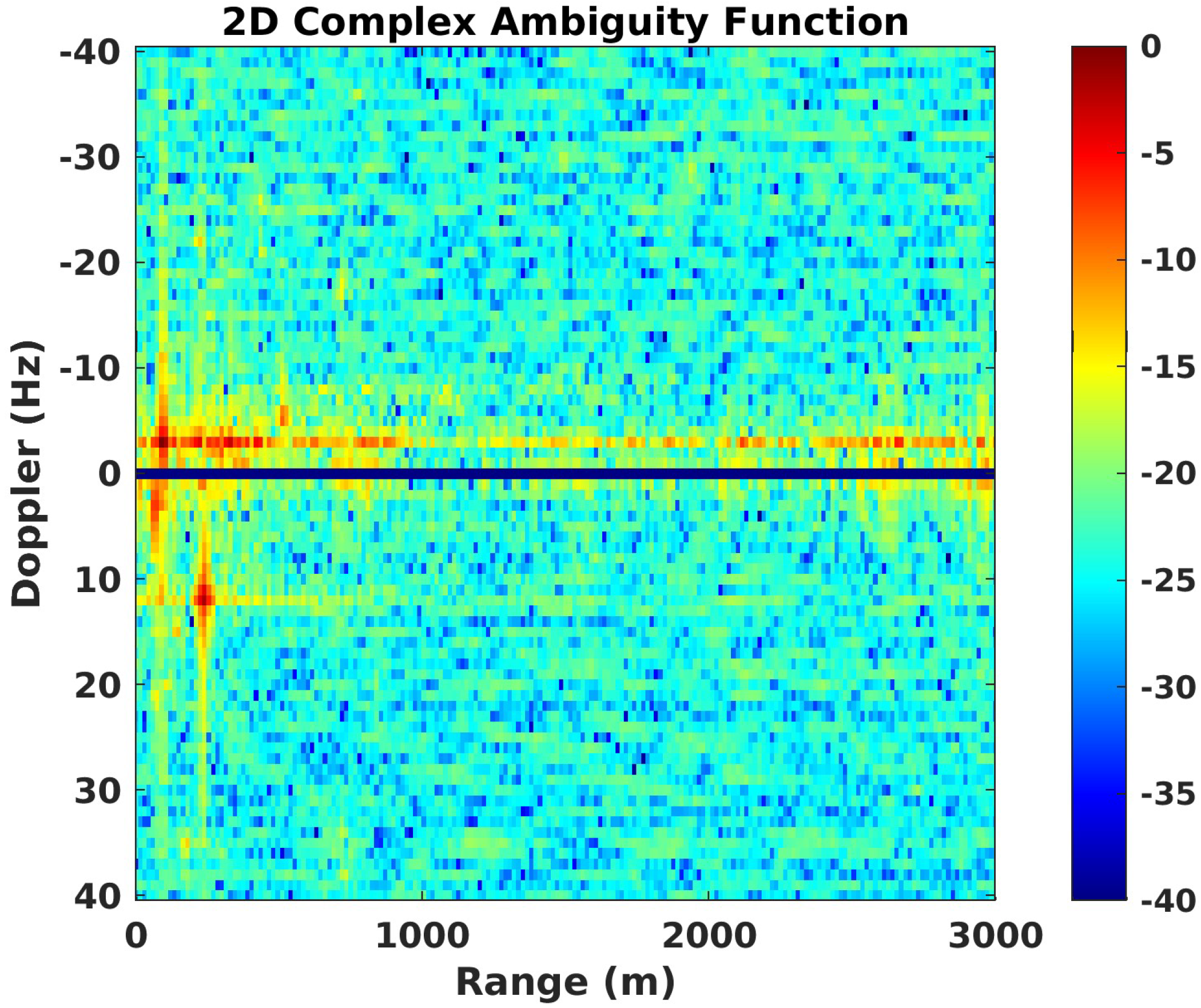
• Passive radar application: the integration of this calibration approach into a passive radar setup successfully enabled the detection and tracking of targets, as evidenced by the range–Doppler and Cartesian coordinate mappings of a vessel within the radar’s coverage area.

Future work may focus on exploring the use of GNSS signals as IoOs. These signals offer unique benefits in terms of consistent availability and worldwide coverage, making them highly promising for passive radar applications. However, integrating GNSS signals will also necessitate the development of specialized calibration techniques to account for their unique characteristics, such as a weaker signal strength, susceptibility to multipath interference, or potential Doppler shifts caused by satellite movement. Addressing these challenges will ensure that the proposed methodology maintains its effectiveness when applied to GNSS-based systems. Additional efforts could include extending the methodology to other array geometries and enhancing LPI techniques to support more demanding covert operation scenarios.

References

- Kuschel, H.; Heckenbach, J.; Muller, S.; Appel, R. On the potentials of passive, multistatic, low frequency radars to counter stealth and detect low flying targets. In Proceedings of the 2008 IEEE Radar Conference, Rome, Italy, 26–30 May 2008; pp. 1–6. [Google Scholar] [CrossRef]
- Kuschel, H.; Cristallini, D.; Olsen, K.E. Tutorial: Passive radar tutorial. IEEE Aerosp. Electron. Syst. Mag. 2019, 34, 2–19. [Google Scholar] [CrossRef]
- Oikonomou, D.; Nomikos, P.G.; Limnaios, G. Passive Radars and their use on the Modern Battlefield. J. Comput. Model. 2019, 9, 37–61. [Google Scholar]
- Fränken, D.; Ott, T.; Lutz, S.; Hoffmann, F.; Samczyński, P.; Płotka, M.; Dróżka, M.; Schüpbach, C.; Mathews, Z.; Welschen, S.; et al. Integrating Multiband Active and Passive Radar for Enhanced Situational Awareness. IEEE Aerosp. Electron. Syst. Mag. 2022, 37, 36–49. [Google Scholar] [CrossRef]
- Bai, L.; Wang, J.; Chen, X. Ambiguity Function Analysis and Side Peaks Suppression of Link16 Signal Based Passive Radar. J. Syst. Eng. Electron. 2023, 34, 1526–1536. [Google Scholar] [CrossRef]
- Olsen, K.E.; Asen, W. Bridging the gap between civilian and military passive radar. IEEE Aerosp. Electron. Syst. Mag. 2017, 32, 4–12. [Google Scholar] [CrossRef]
- Liu, F.; Antoniou, M.; Zeng, Z.; Cherniakov, M. Coherent Change Detection Using Passive GNSS-Based BSAR: Experimental Proof of Concept. IEEE Trans. Geosci. Remote Sens. 2013, 51, 4544–4555. [Google Scholar] [CrossRef]
- Feng, W.; Friedt, J.M.; Nico, G.; Wang, S.; Martin, G.; Sato, M. Passive Bistatic Ground-Based Synthetic Aperture Radar: Concept, System, and Experiment Results. Remote Sens. 2019, 11, 1753. [Google Scholar] [CrossRef]
- Baczyk, M.K.; Samczynski, P.; Krysik, P.; Kulpa, K. Traffic density monitoring using passive radars. IEEE Aerosp. Electron. Syst. Mag. 2017, 32, 14–21. [Google Scholar] [CrossRef]
- Malanowski, M.; Kulpa, K.; Samczynski, P.; Misiurewicz, J.; Kulpa, J. Long range FM-based passive radar. In Proceedings of the IET International Conference on Radar Systems (Radar 2012), Glasgow, UK, 22–25 October 2012; pp. 1–4. [Google Scholar] [CrossRef]
- Palmer, J.E.; Harms, H.A.; Searle, S.J.; Davis, L. DVB-T Passive Radar Signal Processing. IEEE Trans. Signal Process. 2013, 61, 2116–2126. [Google Scholar] [CrossRef]
- Yardley, H.J. Bistatic Radar Based on DAB Illuminators: The Evolution of a Practical System. IEEE Aerosp. Electron. Syst. Mag. 2007, 22, 13–16. [Google Scholar] [CrossRef]
- Zemmari, R.; Nickel, U.; Wirth, W.D. GSM passive radar for medium range surveillance. In Proceedings of the 2009 European Radar Conference (EuRAD), Rome, Italy, 30 September–2 October 2009; pp. 49–52. [Google Scholar]
- Pastina, D.; Santi, F.; Pieralice, F.; Antoniou, M.; Cherniakov, M. Passive Radar Imaging of Ship Targets With GNSS Signals of Opportunity. IEEE Trans. Geosci. Remote Sens. 2021, 59, 2627–2642. [Google Scholar] [CrossRef]
- Zhang, C.; Shi, S.; Yan, S.; Gong, J. Moving Target Detection and Parameter Estimation Using BeiDou GEO Satellites-Based Passive Radar With Short-Time Integration. IEEE J. Sel. Top. Appl. Earth Obs. Remote Sens. 2023, 16, 3959–3972. [Google Scholar] [CrossRef]
- Blázquez-García, R.; Cristallini, D.; Ummenhofer, M.; Seidel, V.; Heckenbach, J.; O’Hagan, D. Capabilities and challenges of passive radar systems based on broadband low-Earth orbit communication satellites. IET Radar Sonar Navig. 2024, 18, 78–92. [Google Scholar] [CrossRef]
- Fabrizio, G.; Colone, F.; Lombardo, P.; Farina, A. Adaptive beamforming for high-frequency over-the-horizon passive radar. IET Radar Sonar Navig. 2009, 3, 384–405. [Google Scholar] [CrossRef]
- Schmidt, R. Multiple emitter location and signal parameter estimation. IEEE Trans. Antennas Propag. 1986, 34, 276–280. [Google Scholar] [CrossRef]
- Zuo, L.; Li, N.; Tan, J.; Peng, X.; Cao, Y.; Zhou, Z.; Han, J. A Coherent Integration Method for Moving Target Detection in Frequency Agile Signal-Based Passive Bistatic Radar. Remote Sens. 2024, 16, 1148. [Google Scholar] [CrossRef]
- Chen, G.; Biao, X.; Jin, Y.; Xu, C.; Ping, Y.; Wang, S. Long-Time Coherent Integration Method for Passive Bistatic Radar Using Frequency Hopping Signals. Sensors 2024, 24, 6236. [Google Scholar] [CrossRef]
- Sorace, R. Phased array calibration. IEEE Trans. Antennas Propag. 2001, 49, 517–525. [Google Scholar] [CrossRef]
- Inoue, Y.; Arai, H. Effect of mutual coupling and manufacturing error of array for DOA estimation of ESPRIT algorithm. Electron. Commun. Jpn. Part I Commun. 2006, 89, 68–76. [Google Scholar] [CrossRef]
- Eberhardt, M.; Eschlwech, P.; Biebl, E. Investigations on antenna array calibration algorithms for direction-of-arrival estimation. Adv. Radio Sci. 2016, 14, 181–190. [Google Scholar] [CrossRef]
- Gupta, I.; Ksienski, A. Effect of mutual coupling on the performance of adaptive arrays. IEEE Trans. Antennas Propag. 1983, 31, 785–791. [Google Scholar] [CrossRef]
- Aumann, H.; Fenn, A.; Willwerth, F. Phased array antenna calibration and pattern prediction using mutual coupling measurements. IEEE Trans. Antennas Propag. 1989, 37, 844–850. [Google Scholar] [CrossRef]
- Babur, G.; Aubry, P.J.; Le Chevalier, F. Antenna Coupling Effects for Space-Time Radar Waveforms: Analysis and Calibration. IEEE Trans. Antennas Propag. 2014, 62, 2572–2586. [Google Scholar] [CrossRef]
- Babur, G.; Manokhin, G.; Monastyrev, E.; Geltser, A.; Shibelgut, A. Simple Calibration Technique for Phased Array Radar Systems. Prog. Electromagn. Res. M 2017, 55, 109–119. [Google Scholar] [CrossRef]
- Knoedler, B.; Zemmari, R. Self-calibration of a passive radar system using GSM base stations. In Proceedings of the 2015 IEEE Radar Conference, Arlington, VA, USA, 10–15 May 2015; pp. 411–416. [Google Scholar] [CrossRef]
- Huang, J.H.; Garry, J.L.; Smith, G.E.; Tan, D.K. In-field calibration of passive array receiver using detected target. In Proceedings of the 2018 IEEE Radar Conference (RadarConf18), Oklahoma City, OK, USA, 23–27 April 2018; pp. 715–720. [Google Scholar] [CrossRef]
- Huang, J.H.; Landon Garry, J.; Smith, G.E. Array-based target localisation in ATSC DTV passive radar. IET Radar Sonar Navig. 2019, 13, 1295–1305. [Google Scholar] [CrossRef]
- Colone, F.; O’Hagan, D.W.; Lombardo, P.; Baker, C.J. A Multistage Processing Algorithm for Disturbance Removal and Target Detection in Passive Bistatic Radar. IEEE Trans. Aerosp. Electron. Syst. 2009, 45, 698–722. [Google Scholar] [CrossRef]
- Nikaein, H.; Zefreh, R.G.; Gazor, S. Target Detection and Interference Cancellation in Passive Radar Sensors via Group-Sparse Regression. IEEE Sens. J. 2023, 23, 21484–21492. [Google Scholar] [CrossRef]
- Prasad, R.; Ojanpera, T. An overview of CDMA evolution toward wideband CDMA. IEEE Commun. Surv. 1998, 1, 2–29. [Google Scholar] [CrossRef]
- Núñez-Ortuño, J.M.; González-Coma, J.P.; Nocelo López, R.; Troncoso-Pastoriza, F.; Álvarez Hernández, M. Beamforming Techniques for Passive Radar: An Overview. Sensors 2023, 23, 3435. [Google Scholar] [CrossRef]
- Malanowski, M.; Kulpa, K. Digital beamforming for Passive Coherent Location radar. In Proceedings of the 2008 IEEE Radar Conference, Rome, Italy, 26–30 May 2008; pp. 1–6. [Google Scholar] [CrossRef]
- Mudumbai, R.; Brown Iii, D.R.; Madhow, U.; Poor, H.V. Distributed transmit beamforming: Challenges and recent progress. IEEE Commun. Mag. 2009, 47, 102–110. [Google Scholar] [CrossRef]
- Trees, H.L.V. Optimum Array Processing; John Wiley & Sons, Ltd.: Hoboken, NJ, USA, 2002. [Google Scholar] [CrossRef]
- ETSI EN 300 744; Digital Video Broadcasting (DVB); Framing Structure, Channel Coding and Modulation for Digital Terrestrial Television. EBU: Grand-Saconnex, Switzerland, 2015. Available online: https://www.etsi.org/deliver/etsi_en/300700_300799/300744/01.06.02_60/en_300744v010602p.pdf (accessed on 27 January 2025).
- Caballero Trenado, L. Spain’s Second Digital Dividend and the Paradox of Broadcasters. Advance 2021, 4, 1–9. [Google Scholar] [CrossRef]
- Sharabati, T. Effect of Pseudo Random Noise (PRN) Spreading Sequence Generation of 3GPP Users’ Codes on GPS Operation in Mobile Handset. J. Commun. Softw. Syst. 2016, 12, 182–189. [Google Scholar] [CrossRef]
- Gold, R. Optimal binary sequences for spread spectrum multiplexing (Corresp.). IEEE Trans. Inf. Theory 1967, 13, 619–621. [Google Scholar] [CrossRef]
- Del-Rey-Maestre, N.; Mata-Moya, D.; Jarabo-Amores, M.P.; Almodóvar-Hernández, A.; Rosado-Sanz, J. DoA techniques in UAV detection with DVB-T based Passive Radar. In Proceedings of the 2023 IEEE International Radar Conference (RADAR), Sydney, Australia, 6–10 November 2023; pp. 1–6. [Google Scholar] [CrossRef]
- Gumminemi, M.; Polipalli, T.R. Implementation of Reconfigurable Transceiver using GNU Radio and HackRF One. Wirel. Pers. Commun. 2020, 112, 889–905. [Google Scholar] [CrossRef]
Disclaimer/Publisher’s Note: The statements, opinions and data contained in all publications are solely those of the individual author(s) and contributor(s) and not of MDPI and/or the editor(s). MDPI and/or the editor(s) disclaim responsibility for any injury to people or property resulting from any ideas, methods, instructions or products referred to in the content. |
© 2025 by the authors. Licensee MDPI, Basel, Switzerland. This article is an open access article distributed under the terms and conditions of the Creative Commons Attribution (CC BY) license (https://creativecommons.org/licenses/by/4.0/).
Share and Cite
González-Coma, J.P.; Nocelo López, R.; Núñez-Ortuño, J.M.; Troncoso-Pastoriza, F. Beacon-Based Phased Array Antenna Calibration for Passive Radar. Remote Sens. 2025, 17, 490. https://doi.org/10.3390/rs17030490
González-Coma JP, Nocelo López R, Núñez-Ortuño JM, Troncoso-Pastoriza F. Beacon-Based Phased Array Antenna Calibration for Passive Radar. Remote Sensing. 2025; 17(3):490. https://doi.org/10.3390/rs17030490
Chicago/Turabian StyleGonzález-Coma, José P., Rubén Nocelo López, José M. Núñez-Ortuño, and Francisco Troncoso-Pastoriza. 2025. "Beacon-Based Phased Array Antenna Calibration for Passive Radar" Remote Sensing 17, no. 3: 490. https://doi.org/10.3390/rs17030490
APA StyleGonzález-Coma, J. P., Nocelo López, R., Núñez-Ortuño, J. M., & Troncoso-Pastoriza, F. (2025). Beacon-Based Phased Array Antenna Calibration for Passive Radar. Remote Sensing, 17(3), 490. https://doi.org/10.3390/rs17030490