Mesosphere and Lower Thermosphere (MLT) Density Responses to the May 2024 Superstorm at Mid-to-High Latitudes in the Northern Hemisphere Based on Sounding of the Atmosphere Using Broadband Emission Radiometry (SABER) Observations

Abstract

The thermospheric density response during geomagnetic storms has been extensively explored, but with limited studies on the density response in the Mesosphere and Lower Thermosphere (MLT) region. In this study, the density response in the MLT region at mid-to-high latitudes of the Northern Hemisphere during the intense geomagnetic storm in May 2024 is investigated using density data from the Sounding of the Atmosphere using Broadband Emission Radiometry (SABER) instrument aboard the Thermosphere Ionosphere Mesosphere Energetics and Dynamics (TIMED) satellite. The results indicate that during the geomagnetic storm, the density response exhibits both significant decreases and increases; specifically, approximately 25.2% of the observation points show a notable reduction within a single day, with the maximum decrease exceeding −59.9% at 105 km. In contrast, around 16.5% of the observation points experience a significant increase over the same period, with the maximum increase surpassing 82.4% at 105 km. The distribution of density changes varies with altitudes. The magnitude of density increases diminishes with decreasing altitude, whereas the density decreases exhibit altitude-dependent intensity variations. Density decreases are primarily concentrated in high-latitude regions, especially in the polar cap, while density increases are mainly observed between 50°N and 70°N. The intensity of density response is generally stronger in the dusk sector than in the dawn sector. These results suggest that atmospheric expansion and uplift driven by temperature variations are the primary factors underlying the observed density change.

1. Introduction

The impact of geomagnetic storms on the neutral density of the Earth’s upper atmosphere was first confirmed by Jacchia [1] using satellite orbital decay data. Since then, the study of thermospheric density response to geomagnetic storms has been a significant focus in upper atmospheric research. Jacchia et al. [2], using orbital drag data from the satellites Injun 3, Explorer 19, and Explorer 24, found a time delay of several hours between the peak of geomagnetic disturbances and the peak of atmospheric disturbances. Roemer [3] further indicated that this delay was independent of latitude, altitude, and local time. Based on data from the low g accelerometer system, Allan [4] reported that during the intense geomagnetic storm of May 1967, three peaks of increased density appeared at magnetic latitudes 0°, 45°, and near the polar cap, while the density around 150 km altitude at magnetic latitude 60° showed a significant decrease. Using the Capteur Accélérométrique Capacitif Triaxial Ultra Sensible (CATUS) accelerometer data, Berger and Barlier [5] found that the density perturbations during geomagnetic storms were more robust in the Northern Hemisphere. Forbes et al. [6] analyzed data from the Satellite Electrostatic Triaxial Accelerometer (SETA) and found that the thermospheric density at an altitude of 200 km increased by 25% during the day and 20% at night in the 45–65° magnetic latitude band as the Kp index rose from 1 to 6. Forbes et al. [7] further reported that the daytime density at high latitudes in summer increased by 50–70% as the Kp index rose from 1–2 to 4–7, while the response in winter high latitudes was relatively weaker. Based on SETA data, Rhoden et al. [8] found that the thermospheric density at 200 km could increase by up to 134% as the Kp index rose from 1 to 6. Bruinsma et al. [9] utilized data from the CHAllenging Minisatellite Payload (CHAMP) and Gravity Recovery and Climate Experiment (GRACE) satellites and reported an increase in thermospheric density of 300–800% during the intense geomagnetic storm of November 2003. Chen et al. [10] conducted a statistical study of corotating interaction region (CIR) and coronal mass ejection (CME) induced geomagnetic storms and found that, although the peak intensity of CIR-induced storms was smaller, their longer duration led to more significant disturbances in thermospheric density. Li and Lei [11], based on the nearly coplanar observations from GRACE and Swarm, reported that during the geomagnetic storms of October 2016 and September 2017, thermospheric density exhibited different hemispheric asymmetries at various altitudes and local times. These studies have further detailed the complex responses of thermospheric density during geomagnetic storms.

Meanwhile, other studies have shown that changes in the thermosphere can propagate to lower altitudes through dynamic and thermodynamic processes [12,13,14], significantly affecting the mesosphere and lower thermosphere (MLT). The MLT region, as the transition zone between the middle and upper atmosphere, is influenced by energy inputs from both the lower and upper atmosphere, which gives rise to unique balancing processes [15,16]. Therefore, exploring the response characteristics of this region during geomagnetic storms is crucial for a comprehensive understanding of the Earth’s atmospheric system. Recent studies have revealed that geomagnetic storms induce significant changes in temperature and winds in the MLT region [17,18,19,20], naturally leading to a change in density. In recent years, the density responses of the MLT region during geomagnetic storms have gradually gained attention, and related studies have emerged. For example, Yi et al. [21] used meteor radar ambipolar diffusion coefficient and temperature data from the MLS satellite to derive density data. They found that during the declining phase of the solar cycle, the density in the mesosphere at altitudes of 85–95 km significantly decreased during geomagnetic activity. Subsequently, Yi et al. [22] conducted further statistical analysis and reported that the mesospheric density in the polar region decreased by more than 10% during geomagnetic storms. These findings indicate that the density response in the MLT region shows significant differences compared to that in the upper thermosphere. This difference may be related to variations in atmospheric properties at different altitudes, with the mechanisms behind these responses, however, not yet fully validated [21]. In addition, observation density data in the MLT region remain limited [23,24], especially considering the altitude gap between the minimum altitude of high-precision satellite in-situ observations and the maximum altitude of stable radar observations, which has resulted in relatively few studies on the density response in the MLT region and significant challenges in providing a comprehensive description and explanation of these responses.

Therefore, utilizing the SABER neutral density data, which cover the previously unobserved 95–110 km range, to study the density response in the MLT region during geomagnetic storms is significant for filling this gap. In this paper, we use SABER density to examine the density response in the MLT region at altitudes between 95 km and 105 km during the May 2024 extreme geomagnetic storm. We describe the May 2024 geomagnetic storm and the TIMED/SABER density data in Section 2; then, we show the density variations in Section 3, followed by the discussion in Section 4 and conclusions in Section 5.

2. Geomagnetic Storm Event and Data

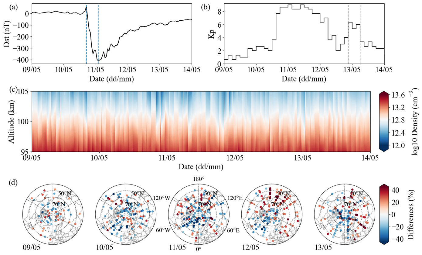
2.1. May 2024 Extreme Geomagnetic Storm

The geomagnetic storm from May 10 to 12, 2024, provides an excellent opportunity to study the MLT density response to superstorms. This storm is the strongest since the Halloween storm of 2003 [25], with a highly standard response process and minimal substorm influence during the recovery phase, making it a textbook example of a geomagnetic storm [26]. Figure 1a,b show geomagnetic activity before and during the storm based on the Dst and Kp indices. After a brief rise, the Dst index begins to decline from 62 nT at 17 UT on May 10, reaching a minimum of −412 nT by 02 UT on May 11, and then gradually starts to recover. The main phase of this geomagnetic storm lasts for 9 h, with the main phase indicated by blue dashed lines in Figure 1a based on the Dst index. The Kp index rises from 4− at 12 UT on May 10, increases to 8− by 15 UT, and reaches its maximum of 9o at 00 UT and 09 UT on May 11. However, during the recovery phase, the Kp index rises again, reaching 6+ at 21 UT on May 12 and 6o at 03 UT on May 13. Concurrently, the Dst index decreases from −83 nT to −102 nT, suggesting the possibility of new intense geomagnetic disturbances during the recovery phase. The gray dashed lines in Figure 1b highlight the periods of intense geomagnetic disturbance during the recovery phase, as defined by the Kp index.

2.2. SABER Density Data

The SABER instrument provides density profiles at 90–110 km altitudes along its orbital path [27], which are derived from its temperature and pressure profiles [28]. These temperature and pressure profiles are retrieved from its CO₂ observations. Although studies on the accuracy of this density data are relatively limited, the temperature data used to calculate density are widely validated [29,30,31], and alternative density profile data at these altitudes are scarce. Therefore, the SABER-derived density data can be reliable for studying density characteristics in the Mesosphere and Lower Thermosphere (MLT) region. Version 2.08 of the Level 2A dataset is used in this study, as it is the latest version available on the SABER website (https://data.gats-inc.com/saber/, accessed on 19 May 2023). Compared to version 2.07, it has resolved anomalies in recent years’ SABER temperature data caused by algorithm instability [32]. Since the density data used in this study are derived from temperature data, version 2.08 can be considered the most suitable SABER observational data for our analysis.

Due to the satellite’s orbit ranging from ~52°S to ~83°N during the geomagnetic storm and the typically weaker density response at mid-to-low latitudes during geomagnetic storms [22], this study primarily focuses on the density changes in the Northern Hemisphere’s mid-to-high latitude MLT region. Given the significant changes in the Kp index starting at 12 UT on 10 May (shown in Figure 1b), we select the preceding two days (from 12 UT on 8 May to 12 UT on 10 May), when the geomagnetic condition was relatively quiet, as the quiet period. The mean values of time, latitude, and longitude for all observation points within each density profile are calculated to represent the spatiotemporal information for that profile. The density values along each profile are then interpolated to obtain density profiles with a vertical resolution of 1 km. Figure 1c illustrates the temporal variation of density within the 65–75°N latitude band, where significant density decreases are observed around 11 May. However, due to the large values of neutral density and substantial variations with altitude, relatively small responses can easily be overlooked in the raw field. To address this, density profiles are assigned to non-overlapping dawn and dusk sector grids of 10° latitude × 20° longitude based on their local time and spatial location (e.g., the dawn grid of 45–55°N, 0–20°E; the dawn grid of 55–65°N, 120–140°W, etc.). For each grid, the mean density profile during quiet periods is calculated as the reference profile. Profiles within the same grid are subtracted by the reference profile and divided by it to obtain the density anomaly percentage profiles. Applying this method across all grids results in the density anomaly percentage profiles for the entire mid-to-high latitude region of the Northern Hemisphere before and after the geomagnetic storm. To ensure all response points reflect significant changes, we apply the same method to density profiles from the same periods in 2020, 2022, and 2023 (when the geomagnetic condition was relatively quiet, with a minimum Dst index of −39 nT and a maximum Kp index of 5+, which can be checked online at https://isgi.unistra.fr/data_plot.php (accessed on 19 April 2023)) to calculate the standard deviation of density changes across latitude bands from 45° to 85°N at 10° intervals. Response points with changes smaller than one standard deviation in each latitude band are considered insignificant. Figure 1d shows the significant response points at 105 km in the mid-to-high latitudes of the Northern Hemisphere (45–83°N) during the pre-storm period on May 9 and the storm period (10–13 May).

2.3. Kernel Density Estimation

Kernel density estimation (KDE) is a non-parametric method for estimating the probability distribution of data, revealing overall trends [33,34]. In this study, to eliminate non-storm factors in the latitude–time distribution of density response, we applied the KDE method to the density scatter points. By placing kernel functions on significant density points in the latitude–time distribution and applying kernel smoothing, we obtained the probability density of these scatter points. These densities were then weighted and summed to produce the final probability density function (PDF) for the entire distribution. Finally, by applying the predefined latitude–time grid to the density function, we generated a visual representation of the function. This visualization allows for a direct comparison of the concentration of scatter points, effectively illustrating the latitudinal distribution of significant atmospheric density responses during the geomagnetic storm.

3. Results

Figure 1c,d reveal that the MLT region exhibits density responses during the geomagnetic storm, including decreases and increases, with distinct characteristics observed across different altitudes, latitudes, and longitudes (local times). These response patterns are further analyzed in the following sections. Due to the relatively large uncertainties associated with SABER observational data near the detection boundaries [30], this study focuses primarily on the 95–105 km range in the MLT region, with 95 km, 100 km, and 105 km selected as the primary altitudes for analysis.

3.1. Time and Altitude Responses of MLT Density

Figure 2 illustrates the changes in the number and intensity of significant response points in the 45–83°N MLT region over time and their proportions among the daily observation points at 105 km, 100 km, and 95 km. It can be seen that some significant points already exist in the mid-to-high latitude MLT region before the storm (9 May). Considering that no sliding average, as performed by Liu et al. [17] and Wang et al. [35], was applied in the data processing, these changes may be caused by non-migrating tides and gravity waves [36,37,38,39]. After the 10th, the number and intensity of response points increase sharply, far exceeding the levels observed before the storm, indicating that density experiences stronger changes under the storm’s influence.

At 105 km, significant density decreases are observed on the 10th and 11th, with the proportion of significant response points reaching 25.2%, indicating extensive density decreases at this altitude. The peak response intensity also exceeds −59.9%. Subsequently, the response begins to weaken on the 12th, with the proportion of significant points and response intensity both decreasing by more than 11.1% from their peaks. In contrast, at 100 km and 95 km, density decreases during the main phase are relatively minor. However, it still reaches a significant level on May 11, indicating a delayed response compared to higher altitudes. The maximum proportion of significant response points reaches 25.5% and 30.3%. Afterward, the response declines slightly, with the reduction remaining below 3.8% on the 12th at 100 km and the 13th at 95 km, reflecting a more prolonged response than higher altitudes. Notably, on May 11, when all three altitudes reach the highest proportion of significant response points, 100 km and 95 km exhibit lower response intensities and higher proportions of significant response points than 105 km. This suggests that the density decreases at these altitudes, covering a broader range while exhibiting lower intensity. Significant density increases, in contrast, are less frequent, though still notable. Some density increases are observed during the main phase, though their number is relatively small. The majority of the density increases occur after the main phase. At 105 km, significant density increases are observed within two days of the main phase, with the proportion of significant points reaching 23.4% and the maximum response intensity exceeding 71.2%. At 100 km and 95 km, the density increases primarily occur 2 to 3 days after the main phase, with the proportion of significant points reaching 15.4% and 14.0%, respectively, and the maximum response intensity exceeding 46.7%. Density decrease intensity weakens with altitude, while the proportion becomes larger at lower altitudes. In contrast, density increases are more pronounced above 100 km, with both proportion and intensity decreasing with altitude. Additionally, density decreases are more numerous despite their lower peak intensity compared to density increases, and both the decreases and increases at lower altitudes generally exhibit delayed responses compared to higher altitudes.

Furthermore, during the recovery phase of the geomagnetic storm on 12–13 May, geomagnetic activity intensified again (as shown in Figure 1b), causing significant density changes in the MLT region. Figure 2 illustrates that between 20 UT on the 12th and 03 UT on the 13th, significant density decreases are observed at 105 km, 100 km, and 95 km, with the maximum response intensity far exceeding that of the previous day. Density increases at 105 km in the latter half of the 13th. While the proportion of significant points declines, the maximum response intensity surpasses that of the previous day. This response process resembles the 10–11 May geomagnetic storm: density decreases during more robust geomagnetic conditions and then increases afterward. However, considering the intensity, duration, and interaction of this geomagnetic activity with the earlier storm, the strength, timing, and affected altitude of density response exhibit some differences. Accordingly, although the density exhibits notable changes during this event, the proportion of significant points continues to decline, with the overall response intensity remaining significantly lower than that during the geomagnetic storm.

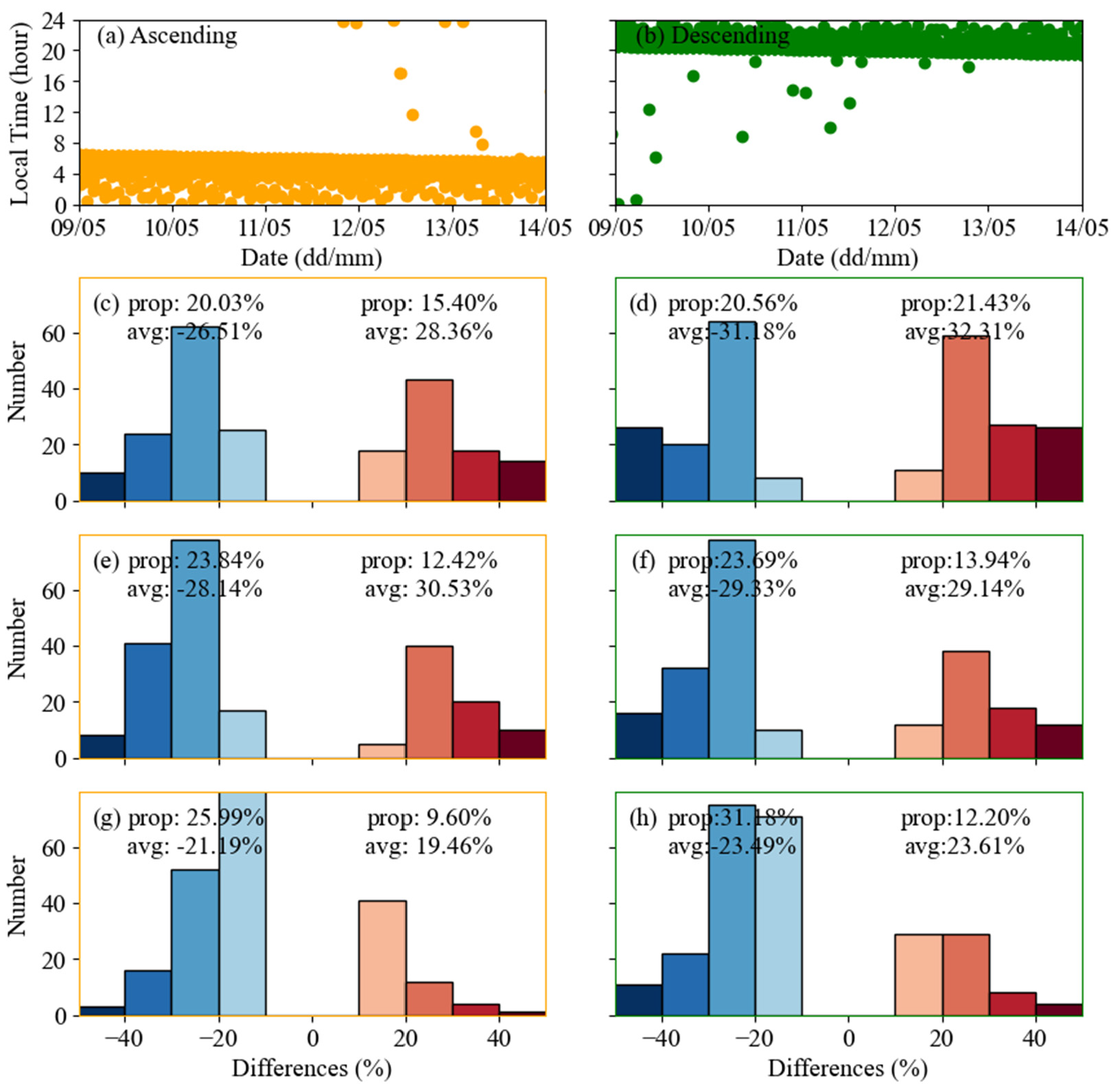
3.2. Latitude and Local Time Responses of MLT Density

The latitude distribution of significant density response points in the 45–83°N MLT region is shown in Figure 3. Considering that non-storm factors (see Figure 2) may persistently influence density and obscure the distribution of significant response points during the storm, we processed the latitude–time scatterplot of significant density response points using the two-dimensional KDE method (see Section 2.3 for details). However, this approach may obscure smaller-scale structures and does not convey specific response intensities or the exact number of significant points. To better highlight the concentrated distribution of significant density response points, we marked the top 10% of the densest regions in the figure. Higher scatter density indicates a more significant response impact in that region. For density decreases, the figure shows dense clusters of significant points at 105 km that emerge above 65°N after the storm’s onset, indicating a more pronounced decrease in density in high-latitude regions. After the main phase, the concentration of significant points diminishes below 77°N while growing above, indicating a contraction of the density decrease range toward higher latitudes. After May 12, significant clusters remain primarily above 77°N, with the response concentrated in the polar cap region (see Figure 1d). At 100 km, dense clusters of density decrease appear between approximately ~77°N and ~82°N after the storm onset, gradually expanding toward lower latitudes. By around May 12, the southernmost extent reaches ~68°N, marking the broadest latitude range of significant density decrease clusters at this altitude. Subsequently, the concentration diminishes, except near ~77°N. This overall process resembles the patterns observed at higher altitude, though it exhibits a delayed response consistent with previously observed conclusions. At 95 km, two dense clusters of density decrease appear after the main phase: one between ~56°N and ~70°N on May 11 and another between ~74°N and ~81°N on 12 May. The former cluster is denser, indicating more significant density decreases in this region. Notably, the dense cluster around ~63°N is also observed at 100 km, albeit with a lower concentration, suggesting a possible vertically weakening density decrease structure extending from lower to higher altitudes near this latitude. This warrants further investigation in future work. For density increases, significant points are notably concentrated below ~70°N across all altitudes. The dense clusters are the most prominent at 105 km, from ~50°N to ~70°N, indicating a broad and significant density increase. As altitude decreases, the concentration and extent of these clusters diminish modestly, shifting slightly toward middle latitudes. The range of the top 10% dense clusters shifts southward from ~47°N to ~64°N at 105 km to ~46°N to ~61°N at 95 km, with the occurrence of significant density increases progressively delayed at lower altitudes.

Figure 4 presents the statistical distribution of significant density response points in the ascending and descending nodes from the onset of the geomagnetic storm at 17 UT on the 10th to the recovery phase on the 14th. These two nodes correspond to the dawn sector (~05:09 LT) and the dusk sector (~20:33 LT). The number in the figure provides the proportion of significant response points and the mean response intensity for density decrease and increase. For density decrease, the intensity is more significant in the dusk sector. The proportion differences at 105 km and 100 km are minimal, at around 0.5% and 0.2%, respectively. However, the greater response intensity in the dusk sector leads to a higher mean response intensity. At 95 km, the proportion of significant decrease in the dusk sector exceeds that in the dawn sector by approximately 5.2%, and more response points with greater intensities result in a greater mean response intensity. For density increase, although the mean response intensity at 100 km is slightly higher in the dawn sector, the proportion of significant response points is greater in the dusk sector across all altitudes, indicating that substantial response points are more frequent in the dusk sector. The most considerable proportion difference is observed at 105 km (~6.0%), which also shows the most significant difference in mean response intensity (~4.0%). This difference between the dawn and dusk sectors will be further discussed in the subsequent section on the mechanisms of density response.

4. Discussion

Section 3 shows that the atmospheric density in the MLT region is significantly affected during this geomagnetic storm. According to the ideal gas law, an increase in temperature corresponds to a decrease in atmospheric density [40]. This process is mainly driven by thermal expansion, which leads to a decrease in the number of molecules per unit volume and, thus, a reduction in density. Conversely, when the temperature decreases and the atmosphere contracts, the density increases. However, since atmospheric density decreases exponentially with altitude and the upper atmosphere is very thin [41], atmospheric expansion or contraction may also affect the density at other altitudes. Fuller-Rowell et al. [42] and Rhoden [8] proposed that enhanced Joule heating in high-latitude regions during geomagnetic storms causes thermal expansion, forming a horizontal pressure gradient. This pressure gradient triggers divergence, driving the upward transport of denser lower atmosphere and increasing thermospheric density. Correspondingly, Yi et al. [21,22] suggested that changes in mesospheric density are due to the energetic particle precipitation from the Earth’s radiation belts into the mesosphere, leading to a decrease in mesospheric ozone and altering the radiative balance, which causes a decrease in both temperature and density. Although the density changes in these studies differ, they all indicate that the density variations during geomagnetic storms are mainly influenced by atmospheric thermal expansion or contraction. Richmond [43] also mentioned in their discussion of thermospheric dynamics during geomagnetic storms that heating effects lead to a temperature increase of several hundred K, causing the thermosphere to expand. Therefore, we suppose that the temperature response in the MLT region during geomagnetic storms is crucial for the density changes.

Banks [44] reported that Joule heating significantly influences the MLT region during geomagnetic storms. Wei et al. [45], through statistical analysis of temperature responses in the MLT region during geomagnetic storms, found that upward vertical winds more significantly influence the dawn sector, while the dusk sector is predominantly affected by downward vertical winds. Consequently, in the dawn sector, Joule heating occurs alongside adiabatic cooling and vertical negative transport caused by upward vertical winds, leading to a counteraction between Joule heating and the cooling effects of vertical winds. This interaction leads to varying temperature responses across different regions, with some areas showing temperature increases and others exhibiting decreases. Conversely, in the dusk sector, Joule heating, combined with adiabatic heating and vertical positive transport due to downward vertical winds, produces a notable temperature increase [46]. We applied the same processing methods to the SABER temperature profiles used for the density profiles to compare the differences between the density and temperature responses during this geomagnetic storm. The results reveal both increases and decreases in temperature during the geomagnetic storm in May 2024. In the dawn sector, weak temperature increases and decreases are observed during the main phase and the following day, gradually developing into intense temperature increases. In contrast, the dusk sector shows dominant temperature increases during the main phase and the following day, with weak decreases observed near the polar region on 12 May. This general pattern is mainly consistent with the findings of Li et al. [47] and Wei et al. [45].

In response to this temperature variation, we propose that, following the onset of the geomagnetic storm, the MLT region at higher altitudes experiences more significant heating. This increase in temperature leads to an atmospheric expansion and a corresponding decrease in density during the main phase and the following day (as shown in the blue part of Figure 2a). Moreover, temperature increases during the geomagnetic storm can influence altitudes as low as 94 km or even lower [17,20]. Liu et al. [17] observed that during geomagnetic storms, the peak temperature response is delayed relative to the AE index, with the delay being shorter at 110 km compared to 105 km. Therefore, we suppose the temperature impact at lower altitudes is similarly delayed. As heating propagates downward, the temperature increase also affects the surrounding atmosphere, leading to a slightly delayed density decrease in these regions (as shown in the blue part of Figure 2b,c). Meanwhile, with the expansion of the atmosphere at lower altitudes, denser air is lifted up, causing density at higher altitudes to gradually shift from decreases to increases (as shown in the red section of Figure 2). This progressive downward response results in a time lag of several hours between density decreases and increases at different altitudes, with lower altitudes showing longer delays (Figure 2). Wang et al. [35] conducted statistical analyses on the impact of CME-induced geomagnetic storms on MLT temperature and found temperature increases at mid-to-high latitudes, with stronger growth at higher altitudes in the polar cap region. This temperature response leads to significant density decreases above 60°N at higher altitudes, with more concentrated decreases near 80°N (blue sections in Figure 3a). Although the temperature response at 65°N is weaker, it influences lower altitudes [35], resulting in more concentrated density decreases near 60°N at 95 km (blue sections in Figure 3c). These density decreases at lower altitudes further contribute to density increases at higher altitudes. Given the exponential decrease in density with altitude, atmospheric regions at higher altitudes are more significantly influenced by the effects of lower atmospheric density. Consequently, above 95 km near 60°N, density increases become more concentrated and intensify with altitude, while the density increase at 95 km itself may be associated with lower layers (red sections in Figure 3). We utilize simulation results from the Ovation Prime model available on the ISWA website (https://iswa.ccmc.gsfc.nasa.gov/IswaSystemWebApp/, accessed on 10 May 2024) and find that during this storm, the auroral oval is primarily concentrated at 55–65°N. Meanwhile, the density shows a stronger decrease in the polar cap region (near 80°N) at higher altitude (blue sections in Figure 3a), which, according to our theory, corresponds to significant temperature variations. In a previous study (Li et al., [47]), where we used the model results to analyze the temperature response to storms at different latitudes, we found that atmospheric heating at 80°N is primarily driven by vertical advection rather than Joule heating. This suggests that the influence of auroral activity on density responses is relatively minor. The differences in density between the dawn and dusk sectors (Figure 4) are mainly controlled by the disparity in temperature response. Since the temperature increase in the dusk sector generally exceeds that in the dawn sector at all altitudes, the density response in the dusk sector tends to exhibit greater response intensities. This process is consistent with the variations observed in most significant density response points, although certain regions exhibit weaker correlations with temperature changes. Li et al. [47] highlighted the significant role of horizontal and vertical transport in temperature variations during geomagnetic storms in the MLT region. Thus, we infer that density responses may not solely result from direct temperature changes but could also be influenced by transport processes associated with wind. It should be mentioned that the mechanism of density changes suggested here is mostly based on speculation; model simulations are needed to verify the mechanism.

5. Conclusions

Using density data from the SABER instrument, we studied the atmospheric density variations and distribution characteristics in the MLT region of the Northern Hemisphere during the extreme geomagnetic storm in May 2024, focusing on the local time distribution of these variations. The main conclusions are as follows:

• Density decreases and increases are observed in the MLT region during the geomagnetic storm. Decreases occur primarily during the main phase and the following day, while increases are mainly observed in the days after the main phase.
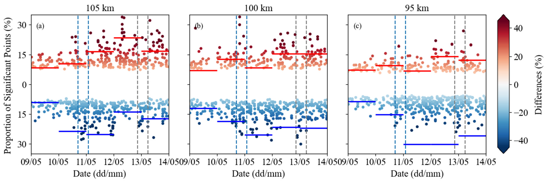
• The response intensity diminishes at lower altitudes, while the delay becomes more pronounced as altitude reduces. The proportion of significant response points varies with altitude: the proportion of decreases is lowest at 105 km (25.2%) and increases as altitude reduces, reaching 30.3% at 95 km. In contrast, the proportion of increases declines from ~16.5% at 105 km to ~14.0% at 95 km.
• Density decreases are primarily observed in two regions: one above 65°N, where the intensity weakens at lower altitudes, and the other near 60°N, where the intensity strengthens as altitude decreases. Density increases are mainly concentrated around 60°N, with a decrease in intensity at lower altitudes.
• Density response during geomagnetic storms is stronger in the dusk sector than in the dawn sector.
• Density response is influenced by atmospheric expansion driven by temperature variations, including a decrease in density caused by local expansion and an increase in density due to the upward displacement of the lower atmospheric expansion.

It is important to note that research on atmospheric density changes in the MLT region during geomagnetic storms remains limited. Further observational statistics and simulation studies are necessary to validate and complement these findings.

References

1. Jacchia, L.G. Two atmospheric effects in the orbital acceleration of artificial satellites. Nature 1959, 18, 526–527. [Google Scholar] [CrossRef]
2. Jacchia, L.G.; Slowey, J.; Verniani, F. Geomagnetic perturbations and upper-atmosphere heating. J. Geophys. Res. 1967, 72, 1423–1434. [Google Scholar] [CrossRef]
3. Roemer, M. Geomagnetic activity effect on atmospheric density in the 250 to 800 km altitude region. Space Res. 1971, 11, 965–974. [Google Scholar]
4. Allan, R.R. Response of dayside thermosphere to an intense geomagnetic storm. Nature 1974, 247, 23–25. [Google Scholar] [CrossRef]
5. Berger, C.; Barlier, F. Asymmetrical structure in the thermosphere during magnetic storms as deduced from the CACTUS accelerometer data. Adv. Space Res. 1981, 1, 231–235. [Google Scholar] [CrossRef]
6. Forbes, J.M.; Roble, R.G.; Marcos, F.A. Magnetic activity dependence of high-latitude thermospheric winds and densities below 200 km. J. Geophys. Res. Space Phys. 1993, 98, 13693–13702. [Google Scholar] [CrossRef]
7. Forbes, J.M.; Gonzalez, R.; Marcos, F.A.; Revelle, D.; Parish, H. Magnetic storm response of lower thermosphere density. J. Geophys. Res. Space Phys. 1996, 101, 2313–2319. [Google Scholar] [CrossRef]
8. Rhoden, E.A.; Forbes, J.M.; Marcos, F.A. The influence of geomagnetic and solar variabilities on lower thermosphere density. J. Atmos. Sol.-Terr. Phys. 2000, 62, 999–1013. [Google Scholar] [CrossRef]
9. Bruinsma, S.; Forbes, J.M.; Nerem, R.S.; Zhang, X. Thermosphere density response to the 20–21 November 2003 solar and geomagnetic storm from CHAMP and GRACE accelerometer data. J. Geophys. Res. Space Phys. 2006, 111, A6. [Google Scholar] [CrossRef]
10. Chen, G.; Xu, J.; Wang, W.; Burns, A.G. A comparison of the effects of CIR- and CME-induced geomagnetic activity on thermospheric densities and spacecraft orbits: Statistical studies. J. Geophys. Res. Space Phys. 2014, 119, 7928–7939. [Google Scholar] [CrossRef]
11. Li, R.; Lei, J. Responses of thermospheric mass densities to the October 2016 and September 2017 geomagnetic storms revealed from multiple satellite observations. J. Geophys. Res. Space Phys. 2021, 126, e2020JA028534. [Google Scholar] [CrossRef]
12. Banks, P.M. Observations of Joule and particle heating in the auroral zone. J. Atmos. Terr. Phys. 1977, 39, 179–193. [Google Scholar] [CrossRef]
13. Rees, M.H.; Emery, B.A.; Roble, R.G.; Stamnes, K. Neutral and ion gas heating by auroral electron precipitation. J. Geophys. Res. 1983, 88, 6289–6300. [Google Scholar] [CrossRef]
14. Roble, R.G.; Emery, B.A.; Killeen, T.L.; Reid, G.C.; Solomon, S.; Garcia, R.R.; Evans, D.S.; Hays, P.B.; Carignan, G.R.; Heelis, R.A.; et al. Joule heating in the mesosphere and thermosphere during the July 13, 1982, solar proton event. J. Geophys. Res. 1987, 92, 6083–6090. [Google Scholar] [CrossRef]
15. Smith, A.K. Global dynamics of the MLT. Surv. Geophys. 2012, 33, 1177–1230. [Google Scholar] [CrossRef]
16. Xu, X.; Manson, A.H.; Meek, C.E.; Chshyolkova, T.; Drummond, J.R.; Hall, C.M.; Riggin, D.M.; Hibbins, R.E. Vertical and interhemispheric links in the stratosphere-mesosphere as revealed by the day-to-day variability of Aura-MLS temperature data. Ann. Geophys. 2009, 27, 3387–3409. [Google Scholar] [CrossRef]
17. Liu, X.; Yue, J.; Wang, W.; Xu, J.; Zhang, Y.; Li, J.; Russell III, J.M.; Hervig, M.E.; Bailey, S.; Nakamura, T. Responses of lower thermospheric temperature to the 2013 St. Patrick’s day geomagnetic storm. Geophys. Res. Lett. 2018, 45, 4656–4664. [Google Scholar] [CrossRef]
18. Lee, Y.S.; Kwak, Y.S.; Kim, K.C.; Kim, Y.H. Dynamically unstable strong wind shears observed in the polar mesosphere summer echo layer associated with geomagnetic disturbances. J. Geophys. Res. Space Phys. 2020, 125, e2019JA027013. [Google Scholar] [CrossRef]
19. Ma, Z.; Gong, Y.; Zhang, S.; Xue, J.; Luo, J.; Zhou, Q.; Huang, C.; Huang, K.; Yu, Y.; Li, G. Study of a Quasi-27-Day Wave in the MLT Region During Recurrent Geomagnetic Storms in Autumn 2018. J. Geophys. Res. Space Phys. 2021, 126, e2020JA028865. [Google Scholar] [CrossRef]
20. Sun, M.; Li, Z.; Li, J.; Lu, J.; Gu, C.; Zhu, M.; Tian, Y. Responses of mesosphere and lower thermosphere temperature to the geomagnetic storm on 7–8 September 2017. Universe 2022, 8, 96. [Google Scholar] [CrossRef]
21. Yi, W.; Reid, I.M.; Xue, X.; Younger, J.P.; Murphy, D.J.; Chen, T.; Dou, X. Response of neutral mesospheric density to geomagnetic forcing. Geophys. Res. Lett. 2017, 44, 8647–8655. [Google Scholar] [CrossRef]
22. Yi, W.; Reid, I.M.; Xue, X.; Murphy, D.J.; Hall, C.M.; Tsutsumi, M.; Ning, B.; Li, G.; Younger, J.P.; Chen, T.; et al. High- and middle-latitude neutral mesospheric density response to geomagnetic storms. Geophys. Res. Lett. 2018, 45, 436–444. [Google Scholar] [CrossRef]
23. Baron, P.; Ochiai, S.; Dupuy, E.; Larsson, R.; Liu, H.; Manago, N.; Murtagh, D.; Oyama, S.; Sagawa, H.; Saito, A.; et al. Potential for the measurement of mesosphere and lower thermosphere (MLT) wind, temperature, density and geomagnetic field with Superconducting Submillimeter-Wave Limb-Emission Sounder 2 (SMILES-2). Atmos. Meas. Tech. 2019, 13, 219–237. [Google Scholar] [CrossRef]
24. Crowley, G. Dynamics of the Earth’s thermosphere: A review. Rev. Geophys. 1991, 29, 1143–1165. [Google Scholar] [CrossRef]
25. Lazzús, J.A.; Salfate, I. Report on the effects of the May 2024 Mother’s day geomagnetic storm observed from Chile. J. Atmos. Sol.-Terr. Phys. 2024, 261, 106304. [Google Scholar] [CrossRef]
26. Spogli, L.; Alberti, T.; Bagiacchi, P.; Cafarella, L.; Cesaroni, C.; Cianchini, G.; Coco, I.; Di Mauro, D.; Ghidoni, R.; Giannattasio, F.; et al. The effects of the May 2024 Mother’s day superstorm over the Mediterranean sector: From data to public communication. Ann. Geophys. 2024, 67, 218. [Google Scholar] [CrossRef]
27. Russell, J.M., III; Mlynczak, M.G.; Gordley, L.L.; Tansock, J.J.; Esplin, R.W. Overview of the SABER experiment and preliminary calibration results. Opt. Spectrosc. Tech. Instrum. Atmos. Space Res. III 1999, 3756, 277–288. [Google Scholar]
28. Cheng, X.; Yang, J.; Xiao, C.; Hu, X. Density correction of NRLMSISE-00 in the middle atmosphere (20–100 km) based on TIMED/SABER density data. Atmosphere 2020, 11, 341. [Google Scholar] [CrossRef]
29. Mlynczak, M.G.; Daniels, T.; Hunt, L.A.; Yue, J.; Marshall, B.T.; Russell, J.M., III; Remsberg, E.E.; Tansock, J.; Esplin, R.; Jensen, M.; et al. Radiometric stability of the SABER instrument. Earth Space Sci. 2020, 7, 1–8. [Google Scholar] [CrossRef]
30. Remsberg, E.E.; Marshall, B.T.; Garcia-Comas, M.; Krueger, D.; Lingenfelser, G.S.; Martin-Torres, J.; Mlynczak, M.G.; Russell, J.M., III; Smith, A.K.; Zhao, Y.; et al. Assessment of the quality of the Version 1.07 temperature-versus-pressure profiles of the middle atmosphere from TIMED/SABER. J. Geophys. Res. Atmos. 2008, 113, D17. [Google Scholar] [CrossRef]
31. Xu, J.; She, C.Y.; Yuan, W.; Mertens, C.; Mlynczak, M.; Russell, J. Comparison between the temperature measurements by TIMED/SABER and lidar in the midlatitude. J. Geophys. Res. Space Phys. 2006, 111, A10. [Google Scholar] [CrossRef]
32. Mlynczak, M.G.; Marshall, B.T.; Garcia, R.R.; Hunt, L.; Yue, J.; Harvey, V.L.; Lopez-Puertas, M.; Mertens, C.; Russell, J.M., III. Algorithm stability and the long-term geospace data record from TIMED/SABER. Geophys. Res. Lett. 2023, 50, e2022GL102398. [Google Scholar] [CrossRef]
33. Chen, Y.C. A tutorial on kernel density estimation and recent advances. Biostat. Epidemiol. 2017, 1, 161–187. [Google Scholar] [CrossRef]
34. Epanechnikov, V.A. Non-parametric estimation of a multivariate probability density. Theory Probab. Its Appl. 1969, 14, 153–158. [Google Scholar] [CrossRef]
35. Wang, N.; Yue, J.; Wang, W.; Qian, L.; Jian, L.; Zhang, J. A comparison of the CIR- and CME-induced geomagnetic activity effects on mesosphere and lower thermospheric temperature. J. Geophys. Res. Space Phys. 2021, 126, e2020JA029029. [Google Scholar] [CrossRef]
36. Hagan, M.E.; Chang, J.L.; Avery, S.K. Global-scale wave model estimates of nonmigrating tidal effects. J. Geophys. Res. Atmos. 1997, 102, 16439–16452. [Google Scholar] [CrossRef]
37. Liu, X.; Yue, J.; Xu, J.; Wang, L.; Yuan, W.; Russell, J.M., III; Hervig, M.E. Gravity wave variations in the polar stratosphere and mesosphere from SOFIE/AIM temperature observations. J. Geophys. Res. Atmos. 2014, 119, 7368–7381. [Google Scholar] [CrossRef]
38. Liu, X.; Yue, J.; Xu, J.; Garcia, R.R.; Russell, J.M., III; Mlynczak, M.; Wu, D.L.; Nakamura, T. Variations of global gravity waves derived from 14 years of SABER temperature observations. J. Geophys. Res. Atmos. 2017, 122, 6231–6249. [Google Scholar] [CrossRef]
39. Xu, J.; Smith, A.K.; Liu, M.; Liu, X.; Gao, H.; Jiang, G.; Yuan, W. Evidence for nonmigrating tides produced by the interaction between tides and stationary planetary waves in the stratosphere and lower mesosphere. J. Geophys. Res. Atmos. 2014, 119, 471–489. [Google Scholar] [CrossRef]
40. Yang, J.; Wang, J.; Liu, D.; Guo, W.; Zhang, Y. Observation and simulation of neutral air density in the middle atmosphere during the 2021 sudden stratospheric warming event. Atmos. Chem. Phys. 2024, 24, 10113–10127. [Google Scholar] [CrossRef]
41. Emmert, J.T. Thermospheric mass density: A review. Adv. Space Res. 2015, 56, 773–824. [Google Scholar] [CrossRef]
42. Fuller-Rowell, T.J.; Codrescu, M.V.; Rishbeth, H.; Moffett, R.J.; Quegan, S. On the seasonal response of the thermosphere and ionosphere to geomagnetic storms. J. Geophys. Res. Space Phys. 1996, 101, 2343–2353. [Google Scholar] [CrossRef]
43. Richmond, A.D.; Lu, G. Upper-atmospheric effects of magnetic storms: A brief tutorial. J. Atmos. Sol.-Terr. Phys. 2000, 62, 1115–1127. [Google Scholar] [CrossRef]
44. Banks, P.M. Joule heating in the high-latitude mesosphere. J. Geophys. Res. Space Phys. 1979, 84, 6709–6712. [Google Scholar] [CrossRef]
45. Wei, G.; Lu, J.; Tang, F.; Li, J.; Sun, M. The dawn-dusk asymmetry in mesosphere and lower thermosphere temperature disturbances during geomagnetic storms at high latitude. Earth Planet. Phys. 2024, 8, 356–367. [Google Scholar] [CrossRef]
46. Yamazaki, Y.; Stolle, C.; Stephan, C.; Mlynczak, M.G. Lower thermospheric temperature response to geomagnetic activity at high latitudes. J. Geophys. Res. Space Phys. 2024, 129, e2024JA032639. [Google Scholar] [CrossRef]
47. Li, J.; Wei, G.; Wang, W.; Luo, Q.; Lu, J.; Tian, Y.; Xiong, S.; Sun, M.; Shen, F.; Yuan, T.; et al. A modeling study on the responses of the mesosphere and lower thermosphere (MLT) temperature to the initial and main phases of geomagnetic storms at high latitudes. J. Geophys. Res. Atmos. 2023, 128, 1–14. [Google Scholar] [CrossRef]
Figure 1. Geomagnetic indices and concurrent SABER density differences from 9 to 13 May 2024. (a) Hourly Dst index. The blue dashed lines indicate the main phase of the storm. (b) Three-hourly Kp index. The gray dashed lines denote intervals of intense geomagnetic disturbances during the recovery phase. (c) Neutral density profiles at 65–75°N. (d) Polar perspective of significant density response points at 105 km, 45–83°N. Points are shown with color representing response intensity, with panels from left to right showing conditions on 9–13 May.
Remotesensing 17 00511 g001
Figure 2. Significant response points in the 45–83°N MLT region from 9 to 13 May 2024. (a) Significant density response points at 105 km. (b,c) are the same as (a), but for altitudes of 100 and 95 km, respectively. The left y-axis indicates the proportion of significant response points relative to the total daily observation points, corresponding to the short horizontal lines in the figure. The red line represents the proportion of significant density increases, while the blue line represents the proportion of density decreases. The point’s color represents the response intensity. The blue dashed line marks the storm’s main phase, and the gray dashed lines denote periods of intense geomagnetic activity during the recovery phase.
Remotesensing 17 00511 g002
Figure 3. Latitude distribution of significant response points in the 45–83°N MLT region from 9 to 13 May 2024. A two-dimensional KDE is applied to the latitude–time distribution of significant points. Color intensity indicates the concentration of points within each region and does not represent specific values. (a) The significant response points at 105 km. (b,c) are the same as (a), but for altitudes of 100 and 95 km, respectively. The upper (red) plots indicate significant density increases and the lower (blue) plots indicate significant decreases. The black dashed lines enclose the densest 10% of significant points. The blue dashed line represents the storm’s main phase and the gray dashed line marks periods of intense geomagnetic disturbance during the recovery phase.
Remotesensing 17 00511 g003
Figure 4. Statistical distribution of significant density response points in the dawn and dusk sectors in the 45–83°N MLT region from 17 UT on 10 to 14 May 2024. (a) The local time distribution of data profiles corresponding to the SABER ascending node. (b) is the same as (a) but for the descending node. (c,e,g) Significant density responses in the dawn sector (orange border) at 105 km, 100 km, and 95 km, respectively. (d,f,h) are the same as (c,e,g), but in the dusk sector (green border). The numbers in the figure represent the proportion (prop) and mean response intensity (avg) for density decreases (blue) and increases (red).
Remotesensing 17 00511 g004
Disclaimer/Publisher’s Note: The statements, opinions and data contained in all publications are solely those of the individual author(s) and contributor(s) and not of MDPI and/or the editor(s). MDPI and/or the editor(s) disclaim responsibility for any injury to people or property resulting from any ideas, methods, instructions or products referred to in the content.