
A Universal Framework for Near-Real-Time Detection of Vegetation Anomalies from Landsat Data

Abstract
1. Introduction
2. Study Area and Landsat Data
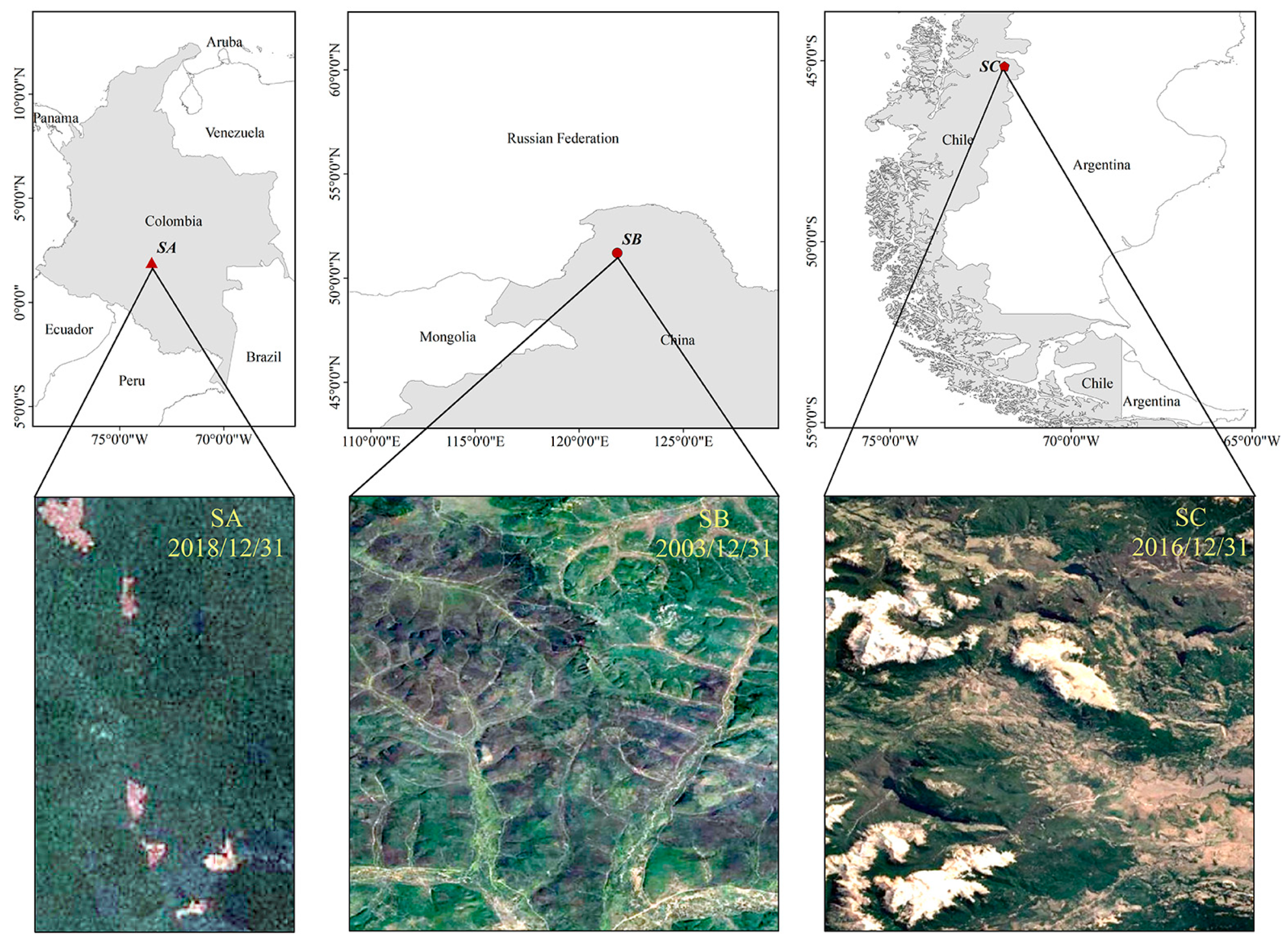
2.1. Study Area
2.2. Landsat Surface Reflectance Product
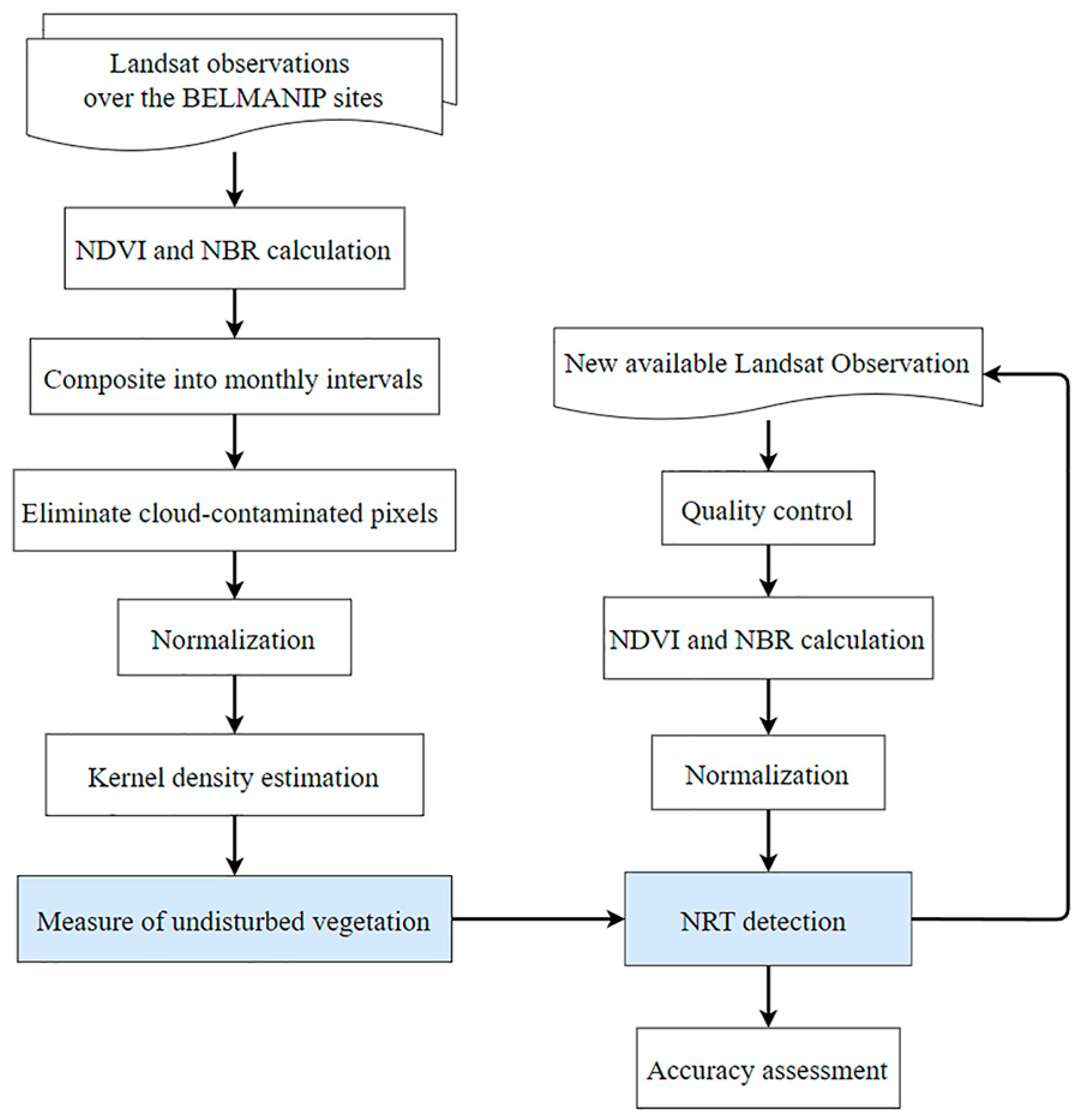
3. Methodology
3.1. Creating the Universal Measure of Undisturbed Vegetation
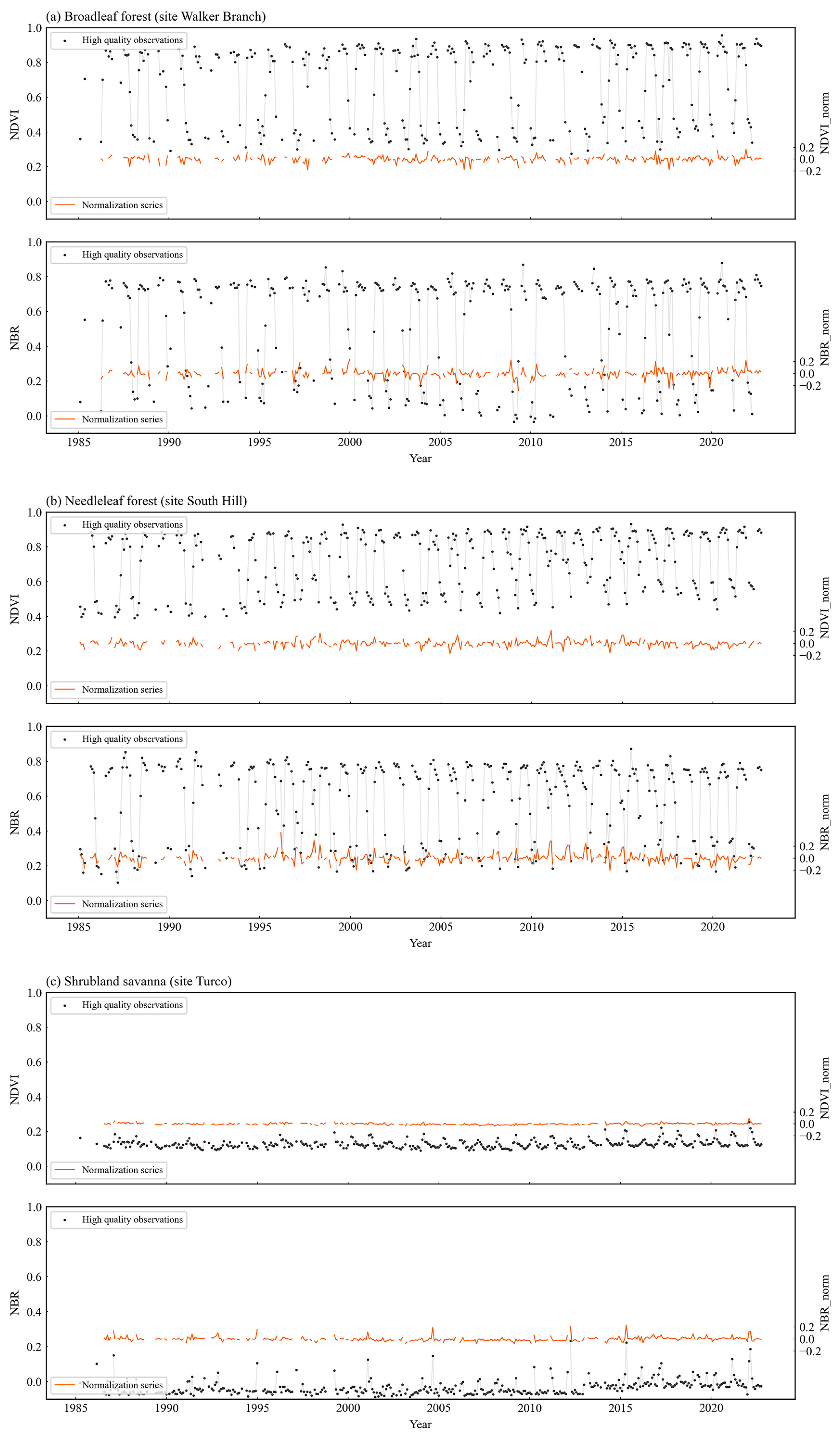
3.1.1. Selection of Reference Data and Vegetation Characteristic Parameters
3.1.2. Elimination of Cloud-Contaminated Pixels
3.1.3. Normalization of NDVI and NBR Values
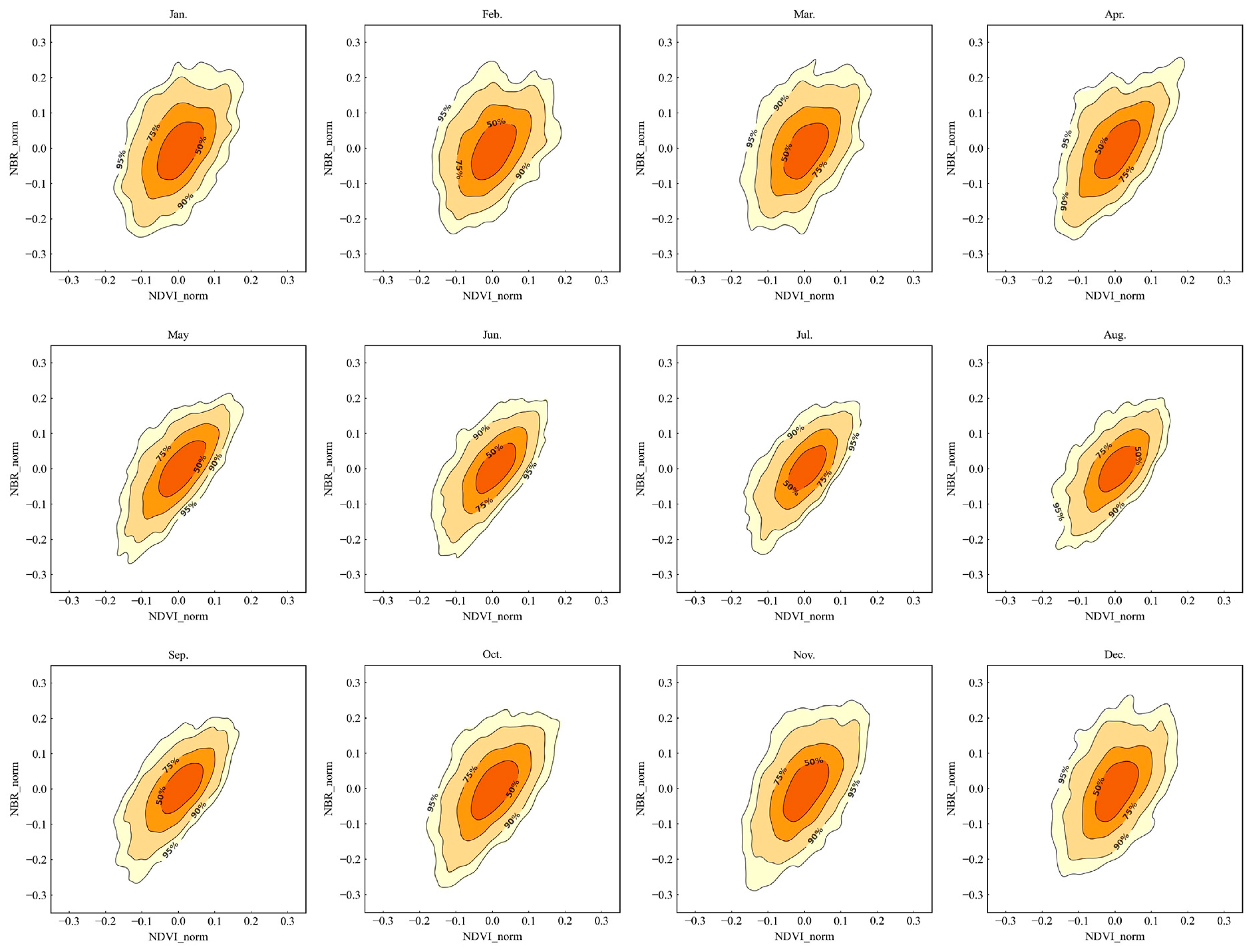
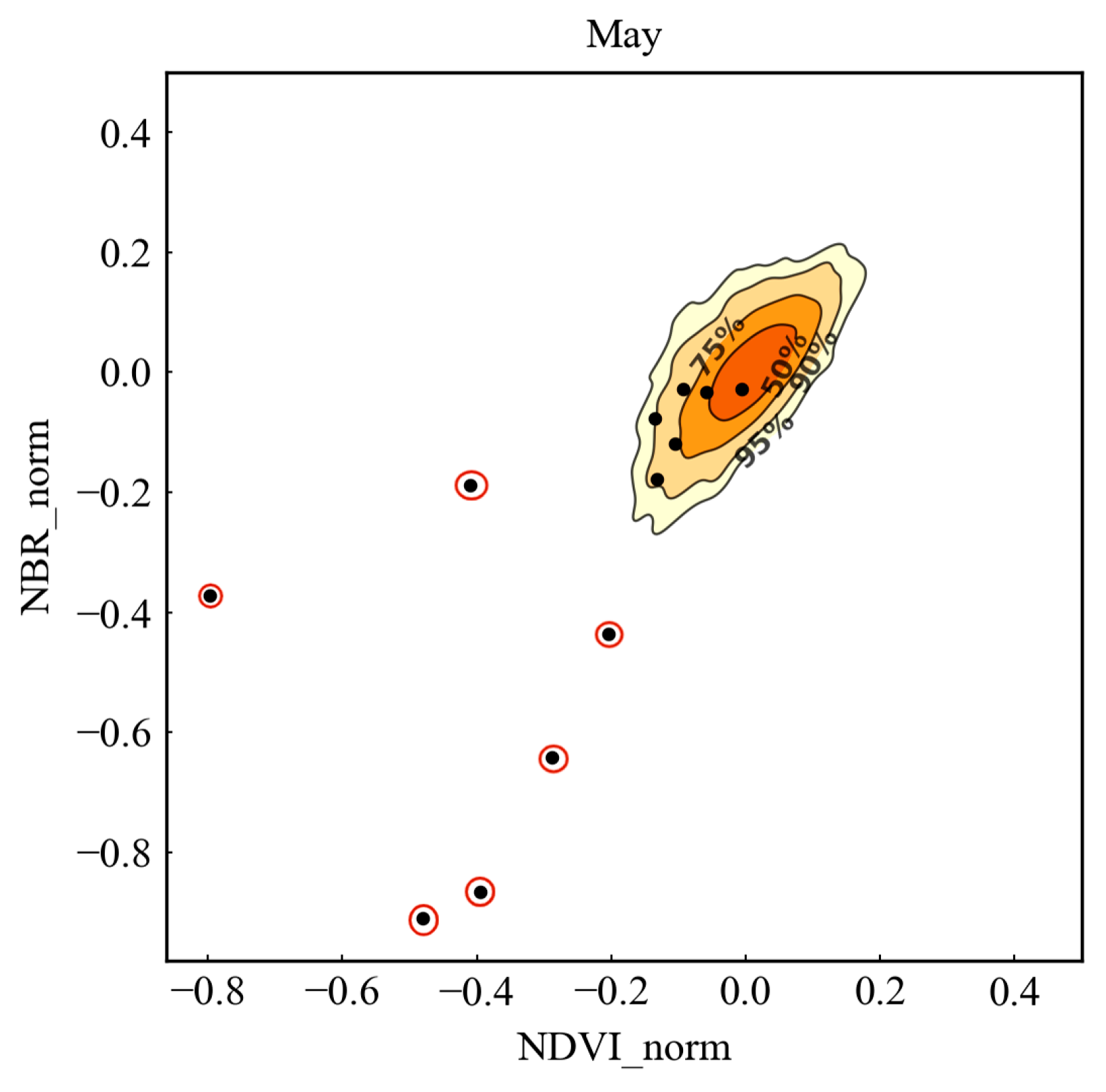
3.1.4. Probability Calculation Based on Kernel Density Estimation
3.2. NRT Vegetation Anomaly Detection
3.3. Accuracy Assessment
3.3.1. Sampling Design
3.3.2. Sample Interpretation and Accuracy Calculation
4. Results
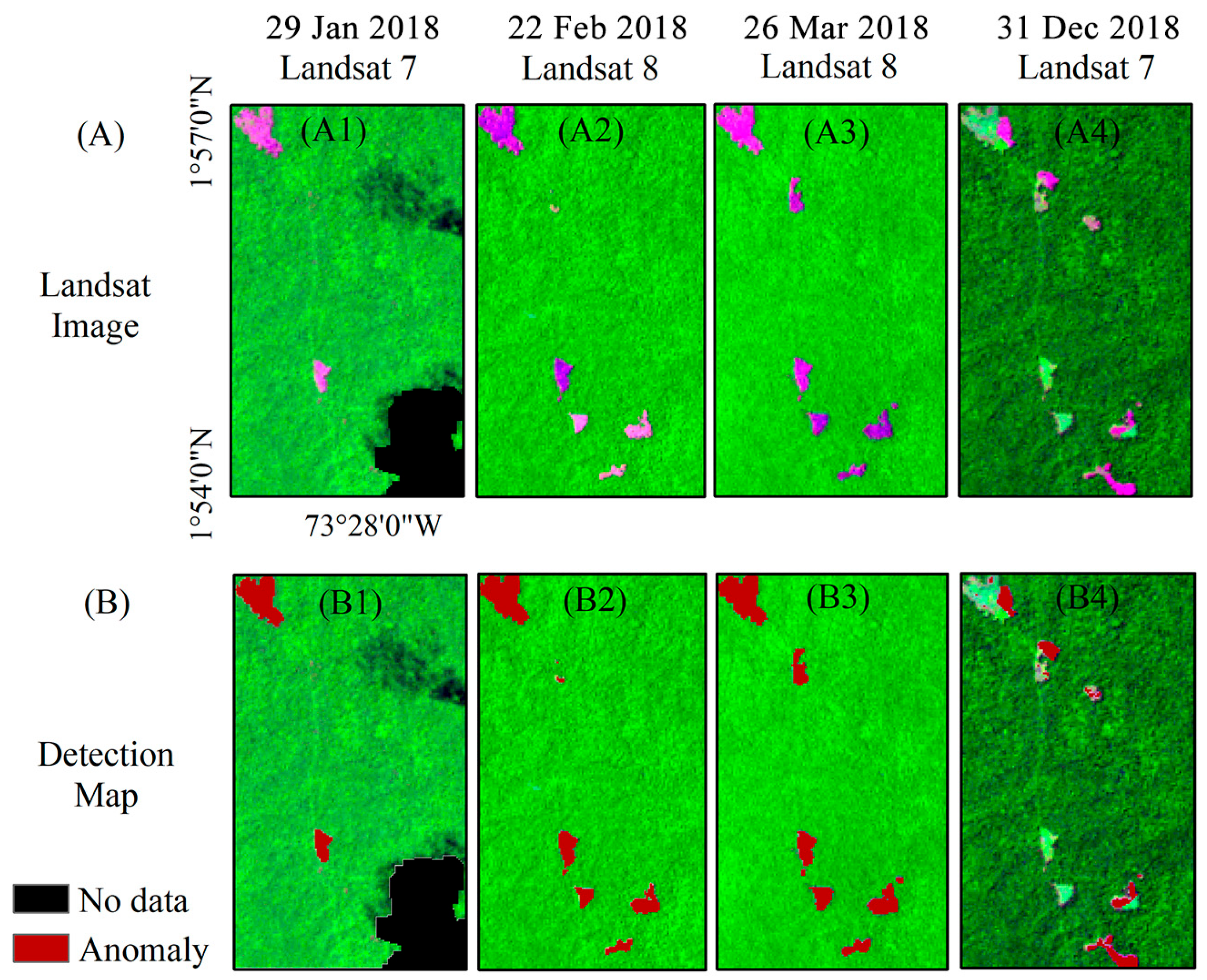
4.1. SA
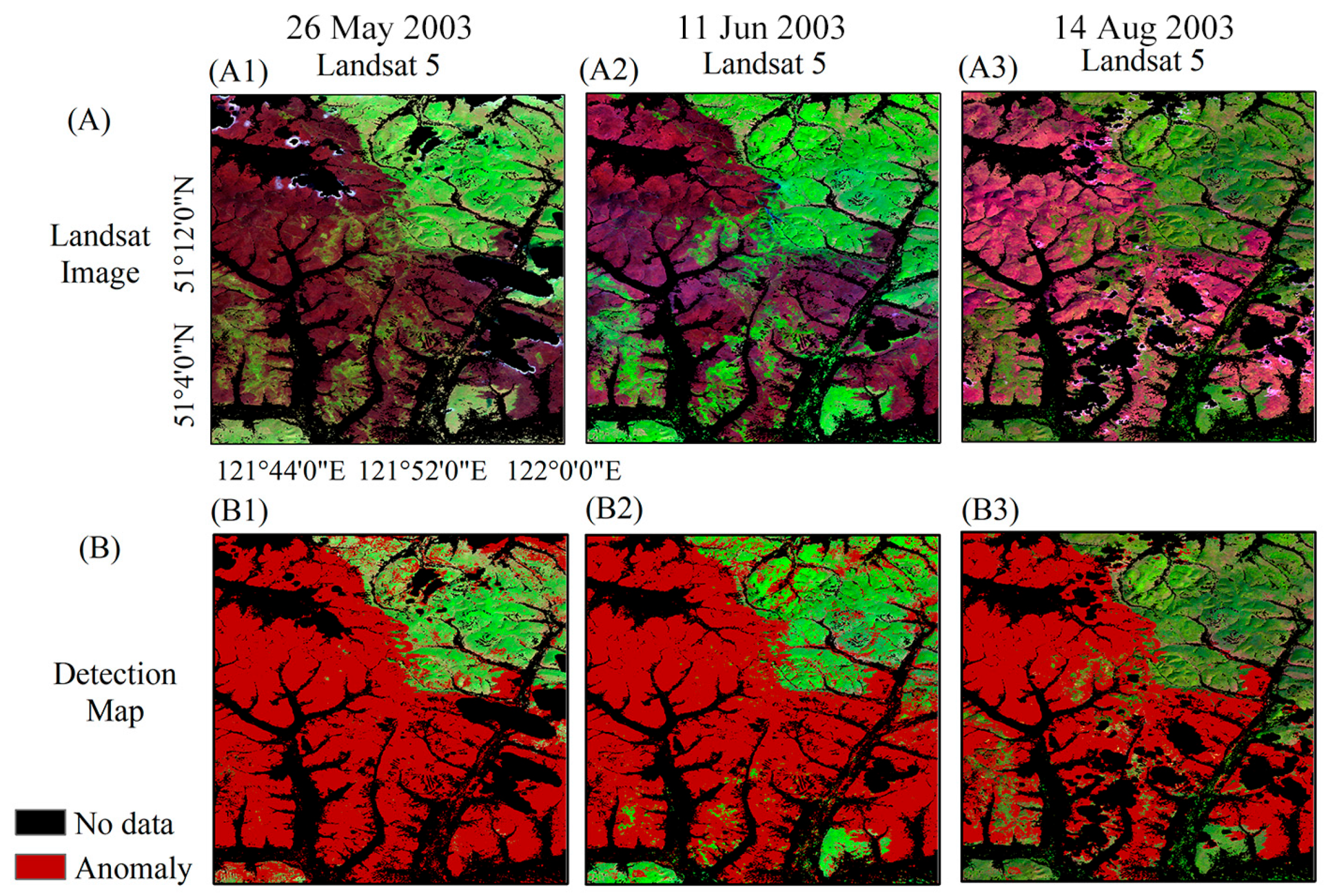
4.2. SB
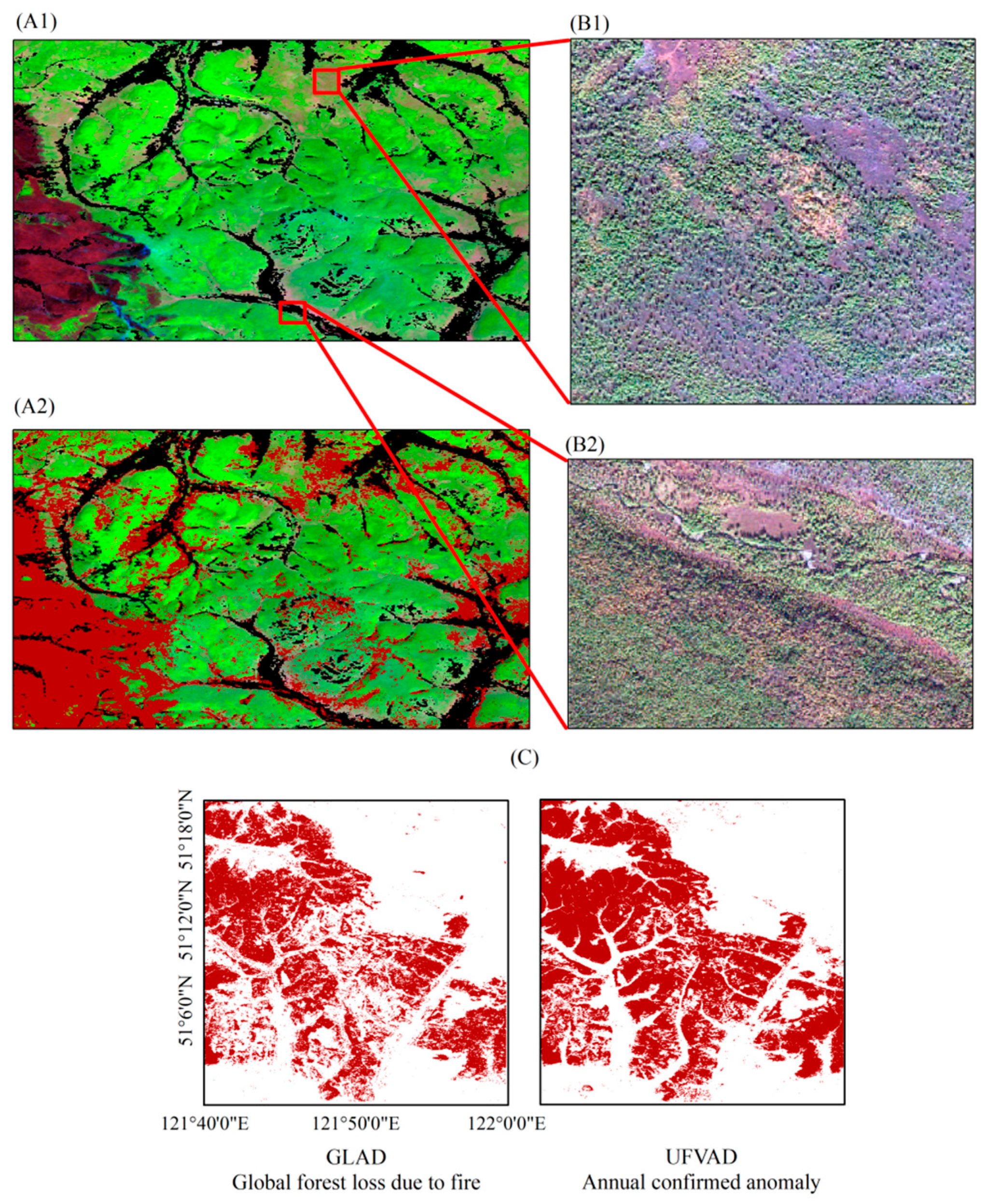
4.3. SC
5. Discussion
5.1. The Robustness of UFVAD in Detecting Different Vegetation Anomalies
5.2. Strength and Defects to UFVAD
5.3. Improvements and Future Plans
6. Conclusions
Author Contributions
Funding
Data Availability Statement
Conflicts of Interest
References
- Chughtai, A.H.; Abbasi, H.; Karas, I.R. A review on change detection method and accuracy assessment for land use land cover. Remote Sens. Appl. Soc. Environ. 2021, 22, 100482. [Google Scholar] [CrossRef]
- Iplak, B. Locust and Grasshopper Outbreaks in the Near East: Review under Global Warming Context. Agronomy 2021, 11, 111. [Google Scholar] [CrossRef]
- Westerling, A.L.; Turner, M.G.; Smithwick, E.A.H.; Romme, W.H.; Ryan, M.G. Continued warming could transform Greater Yellowstone fire regimes by mid-21st century. Proc. Natl. Acad. Sci. USA 2011, 108, 13165–13170. [Google Scholar] [CrossRef] [PubMed]
- Mirza, M.M.Q. Global warming and changes in the probability of occurrence of floods in Bangladesh and implications. Glob. Environ. Change Hum. Policy Dimens. 2002, 12, 127–138. [Google Scholar] [CrossRef]
- Seidl, R.; Thom, D.; Kautz, M.; Martin-Benito, D.; Peltoniemi, M.; Vacchiano, G.; Wild, J.; Ascoli, D.; Petr, M.; Honkaniemi, J.; et al. Forest disturbances under climate change. Nat. Clim. Change 2017, 7, 395–402. [Google Scholar] [CrossRef]
- Grings, F.; Roitberg, E.; Barraza, V. EVI Time-Series Breakpoint Detection Using Convolutional Networks for Online Deforestation Monitoring in Chaco Forest. IEEE Trans. Geosci. Remote Sens. 2020, 58, 1303–1312. [Google Scholar] [CrossRef]
- Hamunyela, E.; Verbesselt, J.; de Bruin, S.; Herold, M. Monitoring Deforestation at Sub-Annual Scales as Extreme Events in Landsat Data Cubes. Remote Sens. 2016, 8, 651. [Google Scholar] [CrossRef]
- Kasischke, E.S.; Turetsky, M.R. Recent changes in the fire regime across the North American boreal region—Spatial and temporal patterns of burning across Canada and Alaska. Geophys. Res. Lett. 2006, 33, 213–222. [Google Scholar]
- Westerling, A.L. Increasing western US forest wildfire activity: Sensitivity to changes in the timing of spring. Philos. Trans. R. Soc. B Biol. Sci. 2016, 371, 20150178. [Google Scholar] [CrossRef] [PubMed]
- Meigs, G.W.; Kennedy, R.E.; Gray, A.N.; Gregory, M.J. Spatiotemporal dynamics of recent mountain pine beetle and western spruce budworm outbreaks across the Pacific Northwest Region, USA. For. Ecol. Manag. 2015, 339, 71–86. [Google Scholar] [CrossRef]
- Paritsis, J.; Veblen, T.T. Dendroecological analysis of defoliator outbreaks on Nothofagus pumilio and their relation to climate variability in the Patagonian Andes. Glob. Change Biol. 2015, 17, 239–253. [Google Scholar] [CrossRef]
- Emanuel, K. Increasing destructiveness of tropical cyclones over the past 30 years. Nature 2005, 436, 686–688. [Google Scholar] [CrossRef]
- Ye, S.; Rogan, J.; Zhu, Z.; Eastman, J.R. A near-real-time approach for monitoring forest disturbance using Landsat time series: Stochastic continuous change detection. Remote Sens. Environ. 2021, 252, 112167. [Google Scholar] [CrossRef]
- Huo, L.; Persson, H.J.; Lindberg, E. Early detection of forest stress from European spruce bark beetle attack, and a new vegetation index: Normalized distance red & SWIR (NDRS). Remote Sens. Environ. 2021, 255, 112240. [Google Scholar]
- Bolton, D.K.; Coops, N.C.; Wulder, M.A. Characterizing residual structure and forest recovery following high-severity fire in the western boreal of Canada using Landsat time-series and airborne lidar data. Remote Sens. Environ. 2015, 163, 48–60. [Google Scholar] [CrossRef]
- Miller, A.B.; Bryant, E.S.; Birnie, R.W. An analysis of land cover changes in the Northern Forest of New England using multitemporal Landsat MSS data. Int. J. Remote Sens. 1998, 19, 245–265. [Google Scholar] [CrossRef]
- Huang, C.; Goward, S.N.; Masek, J.G.; Thomas, N.; Zhu, Z.; Vogelmann, J.E. An automated approach for reconstructing recent forest disturbance history using dense Landsat time series stacks. Remote Sens. Environ. 2010, 114, 183–198. [Google Scholar] [CrossRef]
- Woodcock, C.E.; Macomber, S.A.; Pax-Lenney, M.; Cohen, W.B. Monitoring large areas for forest change using Landsat: Generalization across space, time and Landsat sensors. Remote Sens. Environ. 2001, 78, 194–203. [Google Scholar] [CrossRef]
- Kennedy, R.E.; Yang, Z.; Cohen, W.B. Detecting trends in forest disturbance and recovery using yearly Landsat time series: 1. LandTrendr—Temporal segmentation algorithms. Remote Sens. Environ. 2010, 114, 2897–2910. [Google Scholar] [CrossRef]
- Jamali, S.; Jönsson, P.; Eklundh, L.; Ardö, J.; Seaquist, J. Detecting changes in vegetation trends using time series segmentation. Remote Sens. Environ. 2015, 156, 182–195. [Google Scholar] [CrossRef]
- Verbesselt, J.; Hyndman, R.; Newnham, G.; Culvenor, D. Detecting trend and seasonal changes in satellite image time series. Remote Sens. Environ. 2010, 114, 106–115. [Google Scholar] [CrossRef]
- Smith, V.; Portillo-Quintero, C.; Sanchez-Azofeifa, A.; Hernandez-Stefanoni, J.L. Assessing the accuracy of detected breaks in Landsat time series as predictors of small scale deforestation in tropical dry forests of Mexico and Costa Rica. Remote Sens. Environ. 2019, 221, 707–721. [Google Scholar] [CrossRef]
- Zhao, K.; Wulder, M.A.; Hu, T.; Bright, R.; Wu, Q.; Qin, H.; Li, Y.; Toman, E.; Mallick, B.; Zhang, X.; et al. Detecting change-point, trend, and seasonality in satellite time series data to track abrupt changes and nonlinear dynamics: A Bayesian ensemble algorithm. Remote Sens. Environ. 2019, 232, 111181. [Google Scholar] [CrossRef]
- Rogan, J.; Mietkiewicz, N. Land cover change detection. In Land Resources Monitoring, Modeling, and Mapping with Remote Sensing, 1st ed.; Thenkabail, P.S., Ed.; CRC Press: Boca Raton, FL, USA, 2015; pp. 579–603. [Google Scholar]
- Anees, A.; Aryal, J. Near-Real Time Detection of Beetle Infestation in Pine Forests Using MODIS Data. IEEE J. Sel. Top. Appl. Earth Observ. Remote Sens. 2014, 7, 3713–3723. [Google Scholar] [CrossRef]
- Decuyper, M.; Chávez, R.O.; Lohbeck, M.; Lastra, J.A.; Tsendbazar, N.; Hackländer, J.; Herold, M.; Vågen, T. Continuous monitoring of forest change dynamics with satellite time series. Remote Sens. Environ. 2022, 269, 112829. [Google Scholar] [CrossRef]
- Olsson, P.; Kantola, T.; Lyytikäinen-Saarenmaa, P.; Jönsson, A.M.; Eklundh, L. Development of a method for monitoring of insect induced forest defoliation—Limitation of MODIS data in Fennoscandian forest landscapes. Silva. Fenn. 2016, 50, 1495. [Google Scholar] [CrossRef]
- Pasquarella, V.; Bradley, B.; Woodcock, C. Near-Real-Time Monitoring of Insect Defoliation Using Landsat Time Series. Forests 2017, 8, 275. [Google Scholar] [CrossRef]
- Shang, R.; Zhu, Z.; Zhang, J.; Qiu, S.; Yang, Z.; Li, T.; Yang, X. Near-real-time monitoring of land disturbance with harmonized Landsats 7–8 and Sentinel-2 data. Remote Sens. Environ. 2022, 278, 113073. [Google Scholar] [CrossRef]
- Zhu, Z.; Zhang, J.; Yang, Z.; Aljaddani, A.H.; Cohen, W.B.; Qiu, S.; Zhou, C. Continuous monitoring of land disturbance based on Landsat time series. Remote Sens. Environ. 2019, 238, 111116. [Google Scholar] [CrossRef]
- Verbesselt, J.; Zeileis, A.; Herold, M. Near real-time disturbance detection using satellite image time series. Remote Sens. Environ. 2012, 123, 98–108. [Google Scholar] [CrossRef]
- Zhu, Z.; Woodcock, C.E. Continuous change detection and classification of land cover using all available Landsat data. Remote Sens. Environ. 2014, 144, 152–171. [Google Scholar] [CrossRef]
- Tang, X.; Bullock, E.L.; Olofsson, P.; Estel, S.; Woodcock, C.E. Near real-time monitoring of tropical forest disturbance: New algorithms and assessment framework. Remote Sens. Environ. 2019, 224, 202–218. [Google Scholar] [CrossRef]
- Estay, S.A.; Chávez, R.O. npphen: An R-package for non-parametric reconstruction of vegetation phenology and anomaly detection using remote sensing. BioRxiv 2018, 1, 301143. [Google Scholar]
- Estay, S.A.; Chávez, R.O.; Lastra, J.A.; Rocco, R.; Gutiérrez, A.G.; Decuyper, M. MODIS Time Series Reveal New Maximum Records of Defoliated Area by Ormiscodes amphimone in Deciduous Nothofagus Forests, Southern Chile. Remote Sens. 2023, 15, 3538. [Google Scholar] [CrossRef]
- Estay, S.A.; Chávez, R.O.; Rocco, R.; Gutiérrez, A.G. Quantifying massive outbreaks of the defoliator moth Ormiscodes amphimone in deciduous Nothofagus-dominated southern forests using remote sensing time series analysis. J. Appl. Entomol. 2019, 143, 787–796. [Google Scholar] [CrossRef]
- Chávez, R.O.; Castillo-Soto, M.E.; Traipe, K.; Olea, M.; Lastra, J.A.; Quinones, T. A Probabilistic Multi-Source Remote Sensing Approach to Evaluate Extreme Precursory Drought Conditions of a Wildfire Event in Central Chile. Front. Environ. Sci. 2022, 10, 865406. [Google Scholar] [CrossRef]
- Broich, M.; Huete, A.; Paget, M.; Ma, X.; Tulbure, M.; Coupe, N.R.; Evans, B.; Beringer, J.; Devadas, R.; Davies, K.; et al. A spatially explicit land surface phenology data product for science, monitoring and natural resources management applications. Environ. Modell. Softw. 2015, 64, 191–204. [Google Scholar] [CrossRef]
- Chávez, R.O.; Rocco, R.; Gutiérrez, A.G.; Dörner, M.; Estay, S.A. A Self-Calibrated Non-Parametric Time Series Analysis Approach for Assessing Insect Defoliation of Broad-Leaved Deciduous Nothofagus pumilio Forests. Remote Sens. 2019, 11, 204. [Google Scholar] [CrossRef]
- Tang, X.; Bullock, E.L.; Olofsson, P.; Woodcock, C.E. Can VIIRS continue the legacy of MODIS for near real-time monitoring of tropical forest disturbance? Remote Sens. Environ. 2020, 249, 112024. [Google Scholar] [CrossRef]
- Olsson, P.; Lindström, J.; Eklundh, L. Near real-time monitoring of insect induced defoliation in subalpine birch forests with MODIS derived NDVI. Remote Sens. Environ. 2016, 181, 42–53. [Google Scholar] [CrossRef]
- Hamunyela, E.; Rosca, S.; Mitt, A.; Engle, E.; Herold, M.; Gieseke, F.; Verbesselt, J. Implementation of BFASTmonitor Algorithm on Google Earth Engine to Support Large-Area and Sub-Annual Change Monitoring Using Earth Observation Data. Remote Sens. 2020, 12, 2953. [Google Scholar] [CrossRef]
- Cohen, W.; Healey, S.; Yang, Z.; Stehman, S.; Brewer, C.; Brooks, E.; Gorelick, N.; Huang, C.; Hughes, M.; Kennedy, R.; et al. How Similar Are Forest Disturbance Maps Derived from Different Landsat Time Series Algorithms? Forests 2017, 8, 98. [Google Scholar] [CrossRef]
- Cohen, W.B.; Yang, Z.; Healey, S.P.; Kennedy, R.E.; Gorelick, N. A LandTrendr multispectral ensemble for forest disturbance detection. Remote Sens. Environ. 2018, 205, 131–140. [Google Scholar] [CrossRef]
- Dixon, L. Guaviare: Colombia’s Frontline in the Country’s Battle to Stop Deforestation in the Amazon. Available online: https://news.mongabay.com/2017/05/guaviare-colombias-frontline-in-the-countrys-battle-to-stop-deforestation-in-the-amazon/ (accessed on 8 August 2023).
- University of Maryland and World Resources Institute. Global Primary Forest Loss. Available online: https://www.globalforestwatch.org/dashboards/country/COL/16/ (accessed on 23 February 2024).
- Wu, J.; Liu, Q.; Wang, L.; Chu, G.; Liu, J. Vegetation and climate change during the last deglaciation in the Great Khingan Mountain, Northeastern China. PLoS ONE 2016, 11, e146261. [Google Scholar] [CrossRef] [PubMed]
- Li, Y.; Gao, C.; Liu, H.; Han, D.; Cong, J.; Li, X.; Wang, G. Distribution of phosphorus forms in surface soils of typical peatlands in northern Great Khingan Mountains and its potential to reconstruct paleo-vegetations. J. Environ. Manage. 2022, 302, 114033. [Google Scholar] [CrossRef] [PubMed]
- Veblen, T.T.; Schlegel, F.M.; Oltremari, J.V. Temperate broad-leaved evergreen forests of South America. In Ecosystems of the World; Ovington, J.D., Ed.; Elsevier Science Publishers: Amsterdam, The Netherlands, 1983; pp. 5–31. [Google Scholar]
- Veblen, T.T.; Read, J.; Hill, R.S. The Ecology and Biogeography of Nothofagus Forest. Mt. Res. Dev. 1996, 6, 403. [Google Scholar]
- Masek, J.G.; Goward, S.N.; Kennedy, R.; Cohen, W.B.; Schleweiss, K. United States Forest Disturbance Trends Observed Using Landsat Time Series. Ecosystems 2013, 16, 1087–1104. [Google Scholar] [CrossRef]
- Wulder, M.A.; Masek, J.G.; Cohen, W.B.; Loveland, T.R.; Woodcock, C.E. Opening the archive: How free data has enabled the science and monitoring promise of Landsat. Remote Sens. Environ. 2012, 122, 2–10. [Google Scholar] [CrossRef]
- Ye, S.; Rogan, J.; Sangermano, F. Monitoring rubber plantation expansion using Landsat data time series and a Shapelet-based approach. ISPRS-J. Photogramm. Remote Sens. 2018, 136, 134–143. [Google Scholar] [CrossRef]
- Baret, F.; Morissette, J.T.; Fernandes, R.A.; Champeaux, J.; Myneni, R.B.; Chen, J.; Plummer, S.; Weiss, M.; Bacour, C.; Garrigues, S. Evaluation of the representativeness of networks of sites for the global validation and intercomparison of land biophysical products: Proposition of the CEOS-BELMANIP. IEEE Trans. Geosci. Remote Sens. 2006, 44, 1794–1803. [Google Scholar] [CrossRef]
- Xiao, Z.; Liang, S.; Wang, J.; Chen, P.; Yin, X.; Zhang, L.; Song, J. Use of General Regression Neural Networks for Generating the GLASS Leaf Area Index Product from Time-Series MODIS Surface Reflectance. IEEE Trans. Geosci. Remote Sens. 2014, 52, 209–223. [Google Scholar] [CrossRef]
- Sellers, P.J.; Berry, J.A.; Collatz, G.J.; Field, C.B.; Hall, F.G. Canopy reflectance, photosynthesis, and transpiration. III. A reanalysis using enzyme kinetics- electron transfer models of leaf physiology. Remote Sens. Environ. 1992, 42, 187–216. [Google Scholar] [CrossRef]
- Key, C.H. Ecological and Sampling Constraints on Defining Landscape Fire Severity. Fire Ecol. 2006, 2, 34–59. [Google Scholar] [CrossRef]
- Xiao, Z.; Liang, S.; Tian, X.; Jia, K.; Yao, Y.; Jiang, B. Reconstruction of Long-Term Temporally Continuous NDVI and Surface Reflectance from AVHRR Data. IEEE J. Sel. Top. Appl. Earth Observ. Remote Sens. 2017, 10, 5551–5568. [Google Scholar] [CrossRef]
- Scott, D.W. Multivariate Density Estimation: Theory, Practice, and Visualization, Second Edition. Biometrics 1994, 383, 425. [Google Scholar]
- García-Portugués, E. Notes for Nonparametric Statistics; Carlos III University of Madrid: Madrid, Spain, 2023. [Google Scholar]
- Olofsson, P.; Arevalo, P.; Espejo, A.B.; Green, C.; Lindquist, E.; McRoberts, R.E.; Sanz, M.J. Mitigating the effects of omission errors on area and area change estimates. Remote Sens. Environ. 2020, 236, 111492. [Google Scholar] [CrossRef]
- Cochran, W.G. Sampling Techniques; John Wiley & Sons: New York, NY, USA, 1977. [Google Scholar]
- Olofsson, P.; Foody, G.M.; Herold, M.; Stehman, S.V.; Woodcock, C.E.; Wulder, M.A. Good practices for estimating area and assessing accuracy of land change. Remote Sens. Environ. 2014, 148, 42–57. [Google Scholar] [CrossRef]
- Stehman, S.V.; Wickham, J.D.; Smith, J.H.; Yang, L. Thematic accuracy of the 1992 National Land-Cover Data for the eastern United States: Statistical methodology and regional results. Remote Sens. Environ. 2003, 86, 500–516. [Google Scholar] [CrossRef]
- Hansen, M.C.; Krylov, A.; Tyukavina, A.; Potapov, P.V.; Turubanova, S.; Zutta, B.; Ifo, S.; Margono, B.; Stolle, F.; Moore, R. Humid tropical forest disturbance alerts using Landsat data. Environ. Res. Lett. 2016, 11, 34008–34019. [Google Scholar] [CrossRef]
- Mongolian Forests. Available online: https://www.toursmongolia.com/about-mongolia/mongolian-geography/forest (accessed on 26 January 2025).
- Yan, M.; Li, Z.Y.; Chen, E.X.; Tian, X.; Gu, C.Y.; Li, C.M.; Fan, W.W. Vegetation fractional coverage change in Daxinganling Genhe forest reserve of Inner Mongolia. Chin. J. Ecol. 2016, 35, 508–515. [Google Scholar]
- Hao, X.Y.; Zhang, Z.; Zheng, H.; Gao, N.Z. Detection of spatial and temporal variation characteristics of vegetation cover in the economic zone of the northern slopes of Tianshan Mountains and the influencing factors. China Environ. Sci. 2023, 2023, 1–12. [Google Scholar]
- Brooks, E.B.; Wynne, R.H.; Thomas, V.A.; Blinn, C.E.; Coulston, J.W. On-the-Fly Massively Multitemporal Change Detection Using Statistical Quality Control Charts and Landsat Data. IEEE Trans. Geosci. Remote Sens. 2014, 52, 3316–3332. [Google Scholar] [CrossRef]
- Reiche, J.; Hamunyela, E.; Verbesselt, J.; Hoekman, D.; Herold, M. Improving near-real time deforestation monitoring in tropical dry forests by combining dense Sentinel-1 time series with Landsat and ALOS-2 PALSAR-2. Remote Sens. Environ. 2018, 204, 147–161. [Google Scholar] [CrossRef]
- Tyukavina, A.; Potapov, P.; Hansen, M.C.; Pickens, A.H.; Stehman, S.V.; Turubanova, S.; Parker, D.; Zalles, V.; Lima, A.; Kommareddy, I.; et al. Global Trends of Forest Loss Due to Fire From 2001 to 2019. Front. Remote Sens. 2022, 3, 825190. [Google Scholar] [CrossRef]
- Hansen, M.C.; Potapov, P.V.; Moore, R.; Hancher, M.; Turubanova, S.A.; Tyukavina, A.; Thau, D.; Stehman, S.V.; Goetz, S.J.; Loveland, T.R.; et al. High-Resolution Global Maps of 21st-Century Forest Cover Change. Science 2013, 342, 850–853. [Google Scholar] [CrossRef] [PubMed]
- Huo, L.; Persson, H.J.; Bohlin, J.; Lindberg, E. Green Attack or Overfitting? Comparing Machine-Learning- and Vegetation-Index-Based Methods to Early Detect European Spruce Bark Beetle Attacks Using Multispectral Drone Images. In Proceedings of the IGARSS 2023–2023 IEEE International Geoscience and Remote Sensing Symposium, Pasadena, CA, USA, 16–21 July 2023; pp. 546–549. [Google Scholar]
- Jamali, S.; Olsson, P.O.; Müller, M.; Ghorbanian, A. Kernel-Based Early Detection of Forest Bark Beetle Attack Using Vegetation Indices Time Series of Sentinel-2. IEEE J. Sel. Top. Appl. Earth Observ. Remote Sens. 2024, 17, 12868–12877. [Google Scholar] [CrossRef]
- Ye, S.; Rogan, J.; Zhu, Z.; Hawbaker, T.J.; Hart, S.J.; Andrus, R.A.; Meddens, A.J.H.; Hicke, J.A.; Eastman, J.R.; Kulakowski, D. Detecting subtle change from dense Landsat time series: Case studies of mountain pine beetle and spruce beetle disturbance. Remote Sens. Environ. 2021, 263, 112560. [Google Scholar] [CrossRef]
- Vargas, C.; Montalban, J.; Leon, A.A. Early warning tropical forest loss alerts in Peru using Landsat. Environ. Res. Commun. 2019, 1, 121002. [Google Scholar] [CrossRef]
- Reiche, J.; de Bruin, S.; Hoekman, D.; Verbesselt, J.; Herold, M. A Bayesian Approach to Combine Landsat and ALOS PALSAR Time Series for Near Real-Time Deforestation Detection. Remote Sens. 2015, 7, 4973–4996. [Google Scholar] [CrossRef]
- Mera, D.; Bolon-Canedo, V.; Cotos, J.M.; Alonso-Betanzos, A. On the use of feature selection to improve the detection of sea oil spills in SAR images. Comput. Geosci. 2017, 100, 166–178. [Google Scholar] [CrossRef]
- Sarigai; Yang, J.; Zhou, A.; Han, L.; Xie, Y. Monitoring urban black-odorous water by using hyperspectral data and machine learning. Environ. Pollut. 2021, 269, 116166. [Google Scholar] [CrossRef] [PubMed]
- Lei, L.; Liu, L. Assessment and analysis of collapsing houses by aerial images in the Wenchuan earthquake. J. Remote Sens. 2010, 14, 333–344. [Google Scholar]


| Study Site | Image | Area [Pixels] | Sample Units | |||||
|---|---|---|---|---|---|---|---|---|
| NAOB | NAWB | Anomaly | NAOB | NAWB | Anomaly | Total | ||
| SA | 2018/01/29 | 23,182 | 287 | 460 | 387 | 149 | 238 | 774 |
| 2018/02/22 | 24,451 | 654 | 770 | 454 | 209 | 246 | 909 | |
| 2018/03/26 | 24,142 | 788 | 945 | 455 | 207 | 248 | 910 | |
| 2018/12/31 | 24,888 | 622 | 365 | 453 | 285 | 167 | 905 | |
| SB | 2003/05/26 | 410,829 | 262,393 | 748,247 | 266 | 170 | 436 | 872 |
| 2003/06/11 | 445,815 | 308,065 | 776,289 | 298 | 206 | 505 | 1009 | |
| 2003/08/14 | 698,671 | 193,683 | 542,982 | 337 | 93 | 430 | 860 | |
| SC | 2016/01/08 | 1,367,892 | 79,658 | 22,861 | 431 | 311 | 119 | 861 |
| 2016/02/02 | 1,152,224 | 205,214 | 157,471 | 466 | 268 | 197 | 931 | |
| 2016/03/05 | 1,152,793 | 182,123 | 176,868 | 462 | 245 | 216 | 923 | |
| Strata | NAOB | NAWB | Anomaly | OA (kappa) | UA | PA |
|---|---|---|---|---|---|---|
| SA 29 Jan 2018 | 97.3 (0.96) | |||||
| NAOB | 384 | 0 | 0 | 99.2 | 100.0 | |
| NAWB | 0 | 141 | 10 | 94.6 | 93.4 | |
| Anomaly | 3 | 8 | 228 | 95.8 | 95.4 | |
| SA 22 Feb 2018 | 96.9 (0.95) | |||||
| NAOB | 454 | 0 | 0 | 100.0 | 100.0 | |
| NAWB | 0 | 192 | 11 | 91.9 | 94.6 | |
| Anomaly | 0 | 17 | 235 | 95.5 | 93.3 | |
| SA 26 Mar 2018 | ||||||
| NAOB | 455 | 0 | 0 | 95.9 (0.93) | 100.0 | 100.0 |
| NAWB | 0 | 192 | 22 | 92.8 | 91.1 | |
| Anomaly | 0 | 15 | 226 | 89.7 | 93.8 | |
| SA 31 Dec 2018 | 96.0 (0.94) | |||||
| NAOB | 453 | 0 | 0 | 100.0 | 100.0 | |
| NAWB | 0 | 266 | 17 | 93.3 | 94.0 | |
| Anomaly | 0 | 19 | 150 | 89.8 | 88.8 |
| Strata | NAOB | NAWB | Anomaly | OA (kappa) | UA | PA |
|---|---|---|---|---|---|---|
| SB 26 May 2003 | 89.1(0.82) | |||||
| NAOB | 251 | 0 | 46 | 94.4 | 84.5 | |
| NAWB | 0 | 145 | 9 | 85.3 | 94.2 | |
| Anomaly | 15 | 25 | 381 | 87.4 | 90.5 | |
| SB 11 Jun 2003 | 96.9 (0.95) | |||||
| NAOB | 291 | 0 | 53 | 97.7 | 84.6 | |
| NAWB | 0 | 191 | 9 | 93.2 | 95.5 | |
| Anomaly | 7 | 14 | 443 | 87.7 | 95.5 | |
| SB 14 Aug 2003 | ||||||
| NAOB | 328 | 0 | 14 | 94.7 (0.9) | 97.3 | 95.9 |
| NAWB | 0 | 69 | 4 | 74.2 | 94.5 | |
| Anomaly | 9 | 24 | 412 | 95.8 | 92.6 |
| Strata | NAOB | NAWB | Anomaly | OA (kappa) | UA | PA |
|---|---|---|---|---|---|---|
| SC 8 Jan 2016 | 91.9 (0.87) | |||||
| NAOB | 411 | 0 | 19 | 95.4 | 95.6 | |
| NAWB | 0 | 283 | 3 | 91.0 | 99.0 | |
| Anomaly | 20 | 28 | 97 | 81.5 | 66.9 | |
| SC 2 Feb 2016 | 95.6 (0.93) | |||||
| NAOB | 456 | 0 | 5 | 97.9 | 98.9 | |
| NAWB | 0 | 243 | 1 | 90.7 | 99.6 | |
| Anomaly | 10 | 25 | 191 | 97.0 | 84.5 | |
| SC 5 Mar 2016 | ||||||
| NAOB | 448 | 0 | 2 | 95.9 (0.93) | 97.0 | 99.6 |
| NAWB | 0 | 223 | 0 | 91.0 | 100.0 | |
| Anomaly | 14 | 22 | 214 | 99.1 | 85.6 |
Disclaimer/Publisher’s Note: The statements, opinions and data contained in all publications are solely those of the individual author(s) and contributor(s) and not of MDPI and/or the editor(s). MDPI and/or the editor(s) disclaim responsibility for any injury to people or property resulting from any ideas, methods, instructions or products referred to in the content. |
© 2025 by the authors. Licensee MDPI, Basel, Switzerland. This article is an open access article distributed under the terms and conditions of the Creative Commons Attribution (CC BY) license (https://creativecommons.org/licenses/by/4.0/).
Share and Cite
Xie, Y.; Xiao, Z.; Li, J.; Song, J.; Yang, H.; Lv, K. A Universal Framework for Near-Real-Time Detection of Vegetation Anomalies from Landsat Data. Remote Sens. 2025, 17, 520. https://doi.org/10.3390/rs17030520
Xie Y, Xiao Z, Li J, Song J, Yang H, Lv K. A Universal Framework for Near-Real-Time Detection of Vegetation Anomalies from Landsat Data. Remote Sensing. 2025; 17(3):520. https://doi.org/10.3390/rs17030520
Chicago/Turabian StyleXie, Yixuan, Zhiqiang Xiao, Juan Li, Jinling Song, Hua Yang, and Kexin Lv. 2025. "A Universal Framework for Near-Real-Time Detection of Vegetation Anomalies from Landsat Data" Remote Sensing 17, no. 3: 520. https://doi.org/10.3390/rs17030520
APA StyleXie, Y., Xiao, Z., Li, J., Song, J., Yang, H., & Lv, K. (2025). A Universal Framework for Near-Real-Time Detection of Vegetation Anomalies from Landsat Data. Remote Sensing, 17(3), 520. https://doi.org/10.3390/rs17030520