Abstract
Beach surface moisture (BSM) is crucial to studying coastal aeolian sand transport processes. However, traditional measurement techniques fail to accurately monitor moisture distribution with high spatiotemporal resolution. Remote sensing technologies have garnered widespread attention for providing rapid and non-contact moisture measurements, but a single method has inherent limitations. Passive remote sensing is challenged by complex beach illumination and sediment grain size variability. Active remote sensing represented by LiDAR (light detection and ranging) exhibits high sensitivity to moisture, but requires cumbersome intensity correction and may leave data holes in high-moisture areas. Using machine learning, this research proposes a BSM inversion method that fuses UAV (unmanned aerial vehicle) orthophoto brightness with intensity recorded by TLSs (terrestrial laser scanners). First, a back propagation (BP) network rapidly corrects original intensity with in situ scanning data. Second, beach sand grain size is estimated based on the characteristics of the grain size distribution. Then, by applying nearest point matching, intensity and brightness data are fused at the point cloud level. Finally, a new BP network coupled with the fusion data and grain size information enables automatic brightness correction and BSM inversion. A field experiment at Baicheng Beach in Xiamen, China, confirms that this multi-source data fusion strategy effectively integrates key features from diverse sources, enhancing the BP network predictive performance. This method demonstrates robust predictive accuracy in complex beach environments, with an RMSE of 2.63% across 40 samples, efficiently producing high-resolution BSM maps that offer values in studying aeolian sand transport mechanisms.
1. Introduction
Beaches, which are dynamic coastal landforms, are primarily composed of sediments that are shaped and redistributed by wave action, tides, and wind [1]. Frequent aeolian processes continually reshape the beach environment, with sediments accumulating in the backshore area and eventually developing into coastal dunes. The sediments play a significant role in determining how they respond to dynamic environmental forces and influence the stability and evolution of coastal dunes [2]. Studying aeolian processes is crucial for gaining a deeper understanding of the formation mechanisms of coastal dunes. However, existing aeolian transport prediction models often assume that sediments are transported under ideal conditions, making it difficult to accurately predict sediment transport rates in natural environments [3]. Beach surface moisture (BSM) is an important factor in resisting wind erosion, as the moisture content increases the adhesive forces between sand grains, thereby limiting grain movement and significantly influencing the critical wind speed for sand transport on the beach [4]. Current methods for measuring BSM mainly include manual sampling and remote sensing imagery inversion [5,6]. Nevertheless, the high spatiotemporal variability in BSM can lead to drastic changes from within minutes to hours, making manual sampling inefficient and unable to fully capture the dynamic characteristics of moisture variation. In contrast, remote sensing technologies allow for the rapid inversion of BSM; however, conventional satellite remote sensing imagery is limited by spatial resolution, and is further constrained by weather conditions and satellite overpass intervals, making the real-time high-precision monitoring of target areas challenging. Therefore, the development of efficient and accurate methods for inverting BSM is a key issue in the study of coastal aeolian sand transport processes.
The significant difference in spectral reflectance between dry and wet sand provides a solid physical basis for remote sensing moisture variation [7]. As dry sand becomes wetted, the pore structure between surface sand particles is gradually filled with moisture, resulting in a notable decrease in spectral reflectance, making wet sand appear darker than dry sand.
Digital image technology has been widely used in moisture monitoring research due to its low cost, high resolution, and ease of accessibility. The images of objects contain rich spectral information, and the significant color differences between dry and wet sand make it possible to predict BSM using digital images. Persson [8] quantitatively investigated the relationship between soil color and moisture content, establishing a multivariate linear model for predicting soil moisture based on the S and V parameters in the HSV (Hue, Saturation, Value) color space. Liu [9] proposed a method that combines color information with machine learning to predict soil moisture, finding that brightness parameters demonstrated good predictive performance. Several studies have utilized image brightness for calculating BSM, highlighting the substantial potential of digital image for monitoring spatiotemporal variations in beach moisture [10,11,12]. However, existing research predominantly focuses on homogeneous sediments and often overlooks the influence of sediment grain size on image color.
Compared to digital images, using a terrestrial laser scanner (TLS) is an active remote sensing technique that is largely unaffected by changes in environmental light conditions [13,14,15]. TLSs emit laser beams at specific wavelengths to acquire high-precision three-dimensional coordinate data of targets, while simultaneously recording the backscattered laser intensity, known as “laser intensity”. The intensity value is an important parament for characterizing the spectral reflectance of the target surface [16,17,18]. However, original intensity values are influenced by various factors such as atmospheric effects, instrument characteristics, and scanning geometry (including incidence angle and distance), making it difficult to accurately reflect the true surface properties of the target [19,20]. Tan [21] proposed an empirical model based on the LiDAR equation, assuming that target reflectivity, incidence angle, and scanning distance are independent, and effectively correcting original intensity through polynomial fitting. However, the undulating sand waves present on beach surfaces lead to frequent geometric changes, and existing empirical models require time-consuming indoor and outdoor calibration experiments. This process is cumbersome and may accumulate errors, making it challenging to cope with the complex micro-topographical variations in beaches. Data-driven machine learning algorithms offer new possibilities for correcting intensity. Among these, the back propagation (BP) network is widely used to tackle complex nonlinear problems due to its high adaptability and learning capability, providing a novel solution for the correction and application of intensity data.
Although digital images and TLSs have demonstrated successful applications in moisture monitoring, moisture prediction using a single data source still has its limitations. The complex variations in beach illumination significantly disrupt image brightness, with adverse factors such as vegetation shadows and glare from the specular reflection of seawater directly impacting the results of moisture predictions. While TLS offers advantages in accuracy for moisture monitoring, due to the strong absorption of near-infrared wavelength lasers by water, the TLS produces data holes in high-moisture regions of the intertidal zone. Furthermore, the detection range of the TLS is greatly limited by the installation height of the scanner and the obstructions created by the complex beach environment. Additionally, existing moisture prediction models insufficiently account for the impact of grain size variations on the predicted variables, restricting their applicability in more complex beach settings. An unmanned aerial vehicle (UAV) capable of capturing multi-angle digital images at low altitudes significantly reduces the likelihood of occlusion by terrestrial landcovers [22,23]. Water has a low absorption coefficient in the visible wavelength range, which means that visible light can penetrate through thin layers of water to obtain images of objects at a certain depth underwater [24]. The fusion of digital images and laser point cloud can enhance the robustness of the model, overcoming the deficiencies of data loss and susceptibility to interference associated with a single data source, thereby achieving complete, high-resolution, and high-accuracy inversions of BSM. Moreover, by incorporating information on beach sediment grain size and leveraging the powerful adaptive learning capabilities of BP networks, the influence of grain size variations on the predicted variables can be automatically eliminated, thus broadening the applicability of the moisture prediction model.
Therefore, this paper focuses on the following objectives: (1) Combining machine learning with in situ scanning data of natural beach to propose a rapid correction method for TLS intensity that can cope with the complex micro-geomorphology of beaches. (2) Investigating the impact of sediment grain size on feature parameters such as intensity and image color, and eliminating the interference of grain size variations on predicted variables by incorporating the characteristics of sediment grain size distribution. (3) Through the integration of multi-source data, the key variables for predicting the BSM are screened, and a moisture prediction model with synergistic active and passive remote sensing data are established.
2. Study Site and Data Collection
2.1. Study Site
Baicheng Beach in Xiamen City, Fujian Province, China, was selected as the study site, which is an important part of the National Marine Park in Xiamen and has rich natural and tourism resources (Figure 1). Baicheng Beach is an embayed sand–mud transitional beach located on the western side of the Taiwan Strait, where coastal aeolian sand activities are frequent. The southeastern tip of the beach is composed of granitoid bedrock, while the north-western end is reinforced with artificial seawalls. The wave energy incident onto the beach is relatively high. Wind speed and direction in this area vary significantly with the seasons. During the winter months, the prevailing winds are predominantly from the NE–ENE direction, whereas in the summer, the prevailing winds mainly come from the south. The typical monsoon climate and significant tidal effects result in dynamic changes in the surface moisture of the beach. The natural sediment in this area is primarily sourced from coastal erosion and alongshore sediment transport, with quartz and feldspar being the dominant mineral components. Sand–mud transitional beaches are common along China’s coastline. In recent years, under the influence of extreme weather and high-intensity human activities, beach mudding has intensified [25]. Therefore, studying aeolian sand transport processes on sand–mud transitional beaches is crucial for the protection and management of these areas.
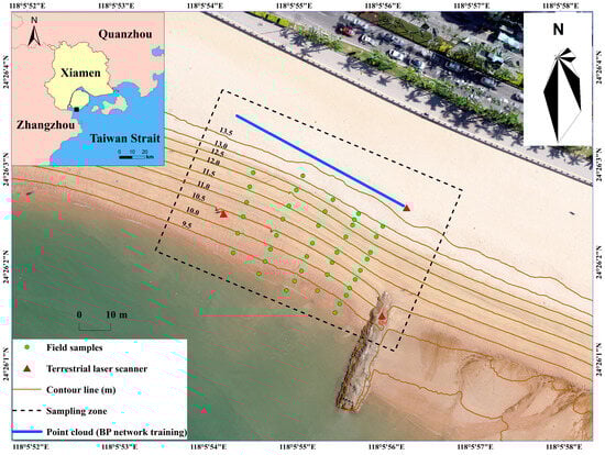
Figure 1.
Field deployment at the Baicheng Beach and the surface moisture sampling points (green). The wind rose was generated based on the average wind frequency for July 2024.
2.2. Data Collection
Data collection for the study site was conducted on 12 July 2024 on a clear and still morning.
2.2.1. Image Acquisition
The Phantom 4 RTK, which was manufactured by DJI (Shenzhen, China), was utilized for image acquisition in this study. The Phantom 4 RTK provides advantages such as stable flight, simple control, and efficient operation, capable of capturing high-definition photos at 20 million pixels and working continuously for approximately 30 min. By connecting to the Qianxun CORS (Continuous Operational Reference System, Qianxun SI Co., Ltd., Shanghai, China), it achieved centimeter-level real-time positioning accuracy.
During data collection, the flight parameters were set with a forward overlap of 75% and a lateral overlap of 60% at an altitude of 60 m. The camera exposure settings were as follows: aperture f/8, ISO 200, and shutter speed 1/320 s. To eliminate the interference of environmental light on image colors, a standard gray card (“Spyder Checkr 24”; Datacolor Co., Ltd., Lawrenceville, GA, USA) and a 24-color standard color card (“Spyder Checkr 24”; Datacolor Co., Ltd., Lawrenceville, GA, USA) were used for white balance and color correction. This process was performed using SpyderCheckr 1.6 software, which enabled the correction of image color distortions caused by changes in light conditions. A total of 166 images were collected. The data were processed using PIX4D software to generate an orthophoto and photogrammetry point cloud for the study site.
2.2.2. Laser Point Cloud Acquisition
The Focus X330 laser scanner, which was manufactured by FARO (Park Lake Mary, Fl, USA), was utilized for laser point cloud collection. This scanner emits near-infrared laser beams at a wavelength of 1550 nm to obtain a point cloud within ranging from 0.6 to 330 m, with a maximum scanning speed of 976,000 pts/s and a measurement accuracy in the millimeter range. The original intensity of each point recorded using the scanner is a dimensionless number that denotes the target reflection level. A high-resolution camera is integrated in the Focus X330 system for an optionally simultaneous color information acquisition.
During data collection, the scanning parameters were set to quality level 2× and resolution 1/2. To save operational time, the color image acquisition process was omitted, and only the grayscale scanning mode was utilized. A total of three stations were assigned for the study site, and four target markers were set up at each two neighbor stations for data registration (Figure 1). RTK (real-time kinematic) equipment was used to record the corresponding coordinates of these target markers for subsequent point cloud coordinate transformation to keep consistency with the orthophoto coordinate system.
2.2.3. Field Sample Collection
Due to the high spatial and temporal variability of BSM, a rectangular area approximately 100 m × 60 m was selected as the sample collection zone to avoid significant changes in beach moisture caused by a time-consuming sample collection process (Figure 1). To prevent interference from the sediment sample collection process on data acquisition, sampling was conducted immediately after the UAV and TLS operations were completed. The size of each sediment sample was controlled to be about 5 cm × 5 cm and 1 cm thick, and the samples were immediately put into sample bags for labeling and sealing to prevent water evaporation. After each sediment sample was collected, RTK equipment recorded the precise location of each sampling point. A total of 40 samples were collected, with sampling points evenly distributed across the sampling zone, effectively reflecting the sediment distribution characteristics of the beach. Upon collection, all samples were immediately transported to the laboratory for moisture content and grain size analyses. Given that the transportation time from field to laboratory was within one hour, the evaporation of the samples was considered negligible. Further information regarding the samples can be found in the Supplementary Materials.
2.3. Calibration Experiment
The data obtained from the calibration experiment were used to develop a moisture prediction model. Twelve samples with different grain sizes were selected from field collections. The samples were placed in glass dishes with a thickness of about 1 cm, and pure water was manually injected into the glass dishes. When the water could no longer penetrate the internal pores of the samples, the samples were considered to have reached saturation moisture. Then, the samples were dried in a constant temperature drying oven at 70 °C. They were taken out every 15 min and weighed, photographed, and scanned until no further changes in mass were observed. This process was repeated 14 times, and 168 images and 144 scanning point clouds of samples with different moisture content were obtained (due to the strong absorption of the near-infrared laser by water, some samples with high water content could not return to the laser beam, resulting in data loss). The moisture content of every sample was calculated using the gravimetric method with the following formula:
where is the moisture content of the sediment, is the mass of the container, is the mass of the container and the wet sample, and is the mass of the container and the dry sample.
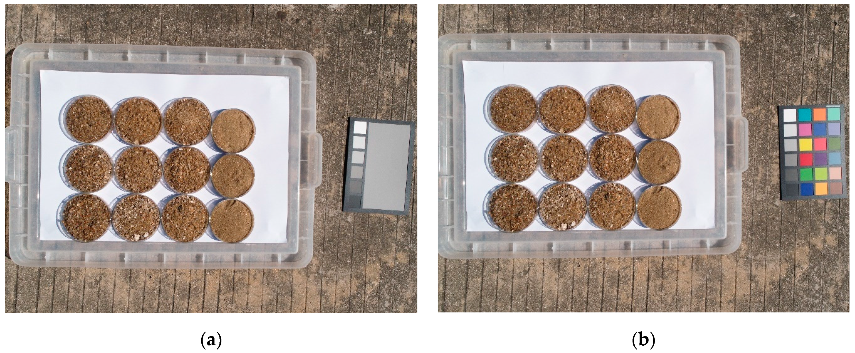
During image collection, to closely simulate the actual UAV aerial photography environment, the Phantom 4 RTK was again used, with the camera parameters set to match those used in flight operations. The images were corrected for white balance and color using a Spyder standard gray card and a 24-color standard color card (Figure 2). When scanning the samples with the TLS, the scanning resolution was set to 1/2, and the point cloud quality was set to 3× to ensure scanning quality.
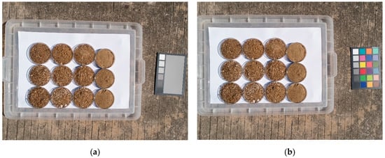
Figure 2.
(a) Samples with different moisture levels with a Spyder standard gray card. (b) Samples with different moisture levels with a Spyder 24-color standard color card (from left to right, the moisture of the samples from top to bottom are 5.87%, 8.27%, 5.39%, 5.28%, 4.36%, 4.35%, 5.94%, 4.21%, 3.09%, 7.17%, 4.61%, and 5.31%).
3. Methods
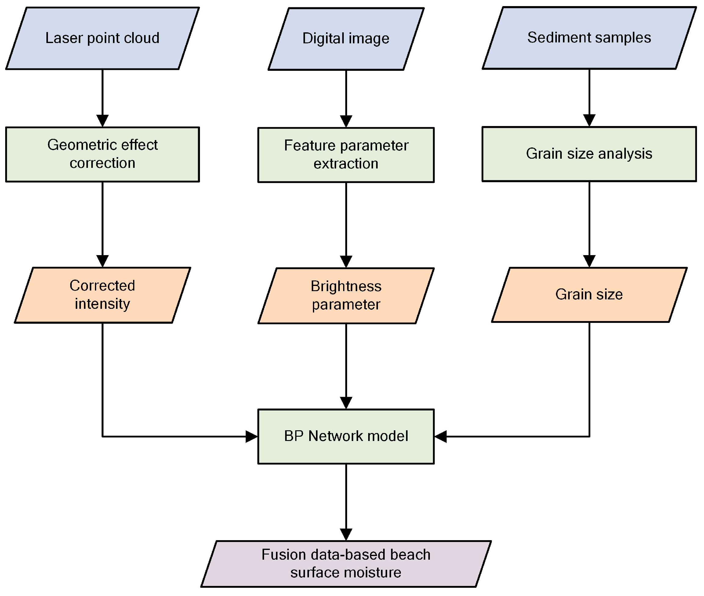
This study establishes a moisture prediction model through calibration experiments and uses remote sensing data from the study site to generate surface moisture distribution on the beach to validate the model’s performance. The workflow is illustrated in Figure 3 and includes the following steps: (a) Data preprocessing (Section 3.1). A BP network is employed to perform intensity correction. Then, the sample grain size is analyzed. (b) Establishing the moisture prediction model (Section 3.2). Feature parameters from multi-source remote sensing data are extracted, screened, and then combined with sediment grain size to achieve automatic image brightness correction and moisture estimation using a new BP network. (c) Model validation (Section 3.3). At the point cloud level, brightness and intensity data fusion is achieved, and the distribution of BSM is estimated by incorporating the characteristics of sediment grain size distribution.
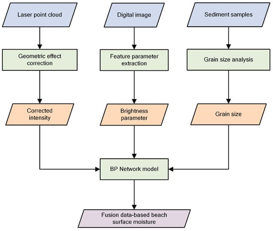
Figure 3.
The workflow of the proposed method.
3.1. Data Preprocessing
3.1.1. Intensity Correction
According to the LiDAR (light detection and ranging) equation, the attenuation of intensity due to atmospheric transmission can be neglected in short- and medium-range scans, and the effects of distance and incidence angle on intensity are independent of each other [21]. Therefore, the intensity can be expressed as follows:
here, is the original intensity, while , , and are functions of target reflectance , incidence angle , and distance , respectively.
To eliminate the effects of incidence angle and distance on the intensity, the corrected intensity is expressed as follows:
where is the reference incidence angle and is the reference distance, and these two values can be specified arbitrarily.
In the beach terrain, the undulating sand ripples cause the incidence angle change frequently and irregularly at different distances, and there are complex nonlinear geometric relationships between and as well as between and . It is difficult to achieve accurate correction of the intensity with single-parameter step-by-step fitting. Therefore, it is necessary to consider the effects of incidence angle and distance on the original intensity at the same time.
The BP (back propagation) network is a mathematical model inspired by the working principle of biological neural systems, which simulates the processing of complex information by the brain. This model consists of many basic units connected to form a complex network, which can be trained by the data to dig out the hidden laws and essential behaviors behind things, without explicitly expressing the physical relationship between multiple parameters, and can handle nonlinear problems well. The basic structure of a BP network includes three components: the input layer, the hidden layer, and the output layer. Each neuron in the network is connected to the previous one via weights and biases, and data analysis on both forward propagation and error backpropagation are performed. This approach enables the BP network to gradually adjust the weights and biases of its connections, allowing for it to perform nonlinear operations and progressively approximate the desired output.
Considering both the incidence angle and distance as geometric parameters, the original intensity can be expressed as follows:
where can be obtained from the BP network training. The corrected intensity can be expressed as follows:
The backshore sand at the study site is fine and dry, making it a homogeneous target with constant reflectivity. The undulating surface of the dry beach introduces a wide range of incidence angles. By using scanned in situ data for intensity correction, cumbersome and time-consuming indoor and outdoor calibration experiments can be avoided. Considering the installation height of the TLS (2.0 m), the point cloud becomes sparse at scanning distance beyond 60 m. Therefore, a strip approximately 60 m in length and 0.2 m in width was selected for training the BP network in the dry beach area to ensure point cloud quality (Figure 1). The incidence angle and distance were treated as inputs, with the corresponding original intensity as the output. BP network training was conducted based on Equation (4) to obtain . With the reference incidence angle and reference distance set, intensity correction was performed according to Equation (5).
3.1.2. Grain Size Analysis
The grain size analysis of the samples was conducted using a POWTEQ SS2000 vibrating sieve, manufactured by Beijing Grinder Instrument Co., Ltd. (Beijing, China), with an amplitude set to 1.0 mm. Each sample was subjected to vibration for 10 min, and the sieve aperture range was from 0.09 mm to 4.00 mm, with a 0.5 difference between each particle size class. Here, is a logarithmic scale based on particle diameter, calculated using the following formula:
where represents the particle diameter (in millimeters). The average particle size of the samples was determined using the Folk–Ward formula, expressed as follows:
here, , , and correspond to the values at the 16%, 50%, and 84% cumulative probability points on the grain size distribution curve, respectively.
3.2. Moisture Prediction Model
3.2.1. Feature Parameter Extraction and Screening
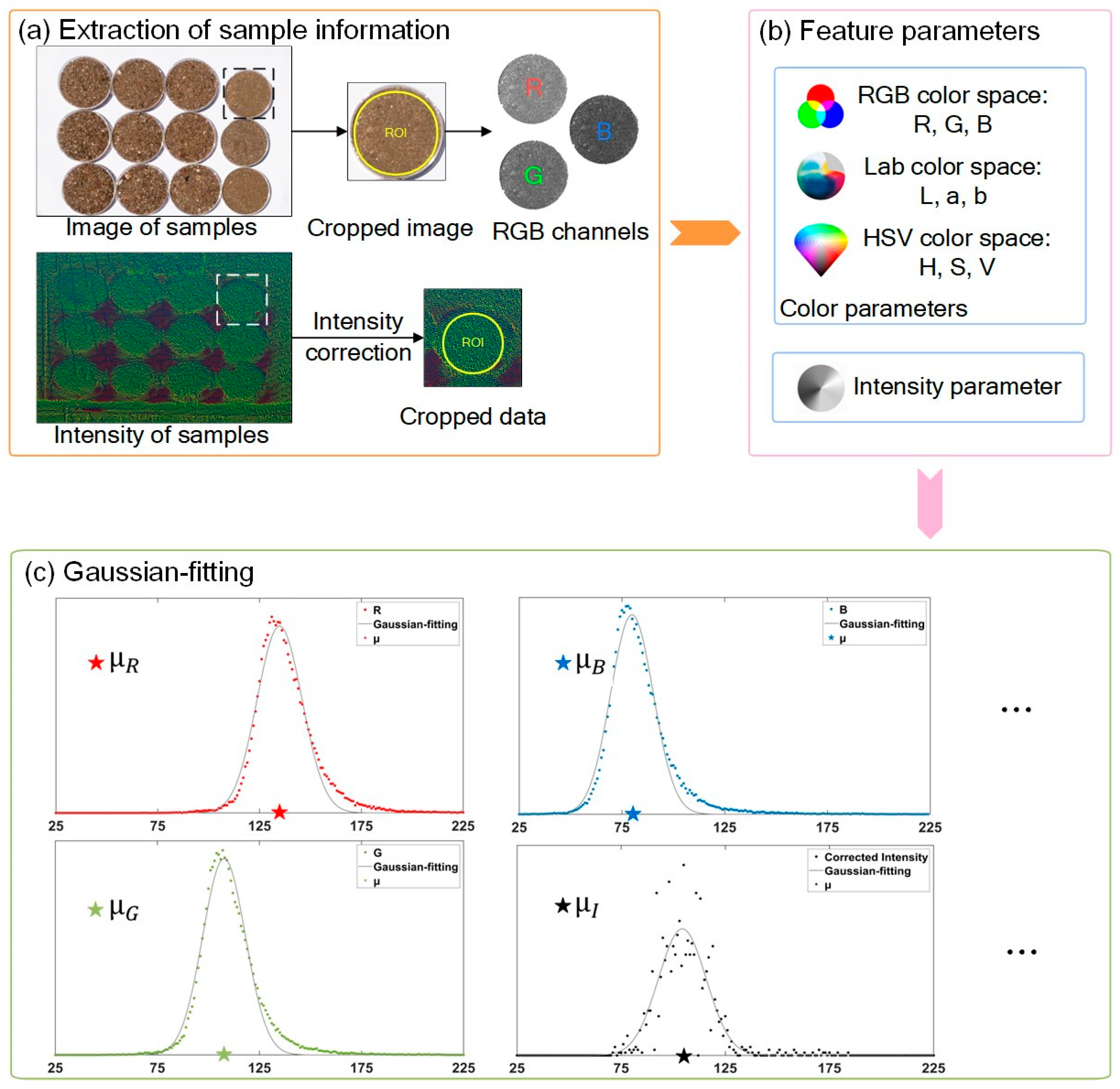
The feature parameter extraction from the sample images and point cloud data obtained in the calibration experiment follows the workflow depicted in Figure 4, which aimed at developing the moisture prediction model. Firstly, the data were cropped to isolate images and point clouds containing only sample information, excluding irrelevant background (Figure 4a). For each sample image, the RGB channels were separated to obtain grayscale images for the R, G, and B channels. Then, to evaluate the predictive capabilities of different color parameters on moisture, the sample images were transformed into the Lab and HSV color spaces. For each sample, 9 grayscale images were generated, each corresponding to one of the 9 color parameters: R, G, B, L, a, b, H, S, and V (Figure 4b). Finally, to reduce the interference from device noise on feature parameter extraction, a Gaussian distribution function—which can more accurately describe the data distribution, reduce the impact of noise and outliers, and provide a more robust and precise mean estimation—was applied to fit the grayscale histogram of each color parameter and intensity, as follows:
where and represent the mean and standard deviation of the Gaussian fit, indicating the overall distribution and dispersion of the sample color or intensity. The mean of the fitted function was selected as the value of the feature parameter of the sample (Figure 4c).
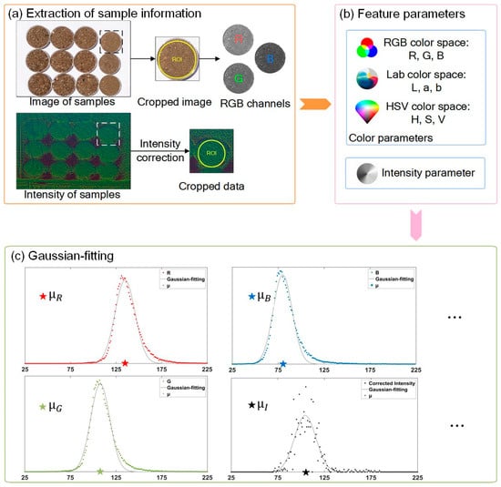
Figure 4.
The process of feature parameter extraction: (a) Extraction of sample information; (b) acquisition of feature parameters; (c) Gaussian-fitting the histogram of color parameters and intensity parameters.
In order to improve the prediction ability of the model, it is necessary to screen for the feature parameters that are sensitive to moisture changes. However, many parameters may be highly correlated across different color spaces; screening the feature parameters can reduce data redundancy and enhance the generalization ability of the model. The correlation coefficient quantifies the linear relationship between the dependent variable and each predictor variable. In this study, a Pearson correlation coefficient matrix was calculated between 10 feature parameters (9 color parameters and 1 intensity parameter) and moisture to identify the parameters strongly correlated with moisture changes for subsequent modeling.
3.2.2. BP Network Model
In predicting BSM using multiple parameters, complex nonlinear relationships among different data sources make it difficult to establish a clear mathematical model. Therefore, a BP network is employed for multivariable parameter modeling. After screening, the intensity I and the brightness V (from the HSV color space), which exhibit the strongest correlation with moisture variation, are selected as predictor variables (more details in Section 4.3). However, sediment grain size significantly affects image brightness (more details in Section 5.2). Thus, grain size is included as a correction parameter in the model. The powerful adaptive learning ability of the BP network is utilized to achieve the automatic correction of image brightness. The formula is as follows:
here, is the moisture content of the sample, is the corrected intensity, is the image brightness, and is the average grain size of the sample. For samples with high moisture lacking intensity data, set .
The 168 sample point clouds obtained from the calibration experiment were used to train the . The data were divided into two parts: 70% for the training set, and 30% for the testing set.
3.3. Model Validation
3.3.1. Data Fusion
The laser point cloud obtained from TLS and the images acquired by the UAV are data of different dimensions and sources and thus cannot be directly fused. The photogrammetry point cloud derived from the images preserves the original color of the objects while also restoring their three-dimensional coordinates, which provides a possibility for data fusion at the point cloud level. Firstly, the intensity of the laser point cloud is corrected, and the brightness of the photogrammetry point cloud is converted. Then, the Iterative Closest Point (ICP) algorithm is applied to accurately register the laser point cloud and the photogrammetry point cloud, calculating the average distance between them. Finally, each point in the photogrammetry point cloud is traversed to find the nearest point in the laser point cloud. If the distance between the two points is less than the average distance, the intensity of the nearest point is assigned to the corresponding point, thereby achieving data fusion at the point cloud level. To address holes caused by the missing laser point cloud, the photogrammetry point cloud is used to fill these voids, with the intensity I assigned a value of 0. This process is implemented through MATLAB programming.
3.3.2. Grain Size Estimation
In the beach foreshore, sediment grain size shows a significant linear relationship with distance to the beach berm (more details in Section 4.2). Therefore, the sediment grain size in the foreshore area is estimated based on the distance to the beach berm. The estimation formula was obtained by fitting the average grain size of the 40 sediment samples collected in the field to the distance between the sampling point and the beach berm, as follows:
where represents the average grain size of the samples and is the distance from the sampling point to the beach berm.
Sediments in the backshore are primarily transported by wind, resulting in a fine and uniformly distributed grain size. Therefore, in the fused point cloud of the backshore region, each point is randomly assigned a grain size between 0.1~0.3 mm to accurately reflect the actual grain size distribution.
4. Results
4.1. Results of Intensity Correction
After denoising and subsampling the original point cloud using the open-source software CloudCompare 2.12.4, a total of 9,228,603 points were obtained. The intensity correction of the point cloud was performed using a reference incident angle of and a reference distance of ds = 8 m.
Figure 5a illustrates the original intensity distribution of the point cloud, with red indicating high-intensity regions and blue representing low-intensity regions, where high-reflection-intensity regions are concentrated in the backshore. These regions are characterized by dry sand with extremely low moisture, resulting in an extensive red area. Conversely, low-reflection-intensity regions are primarily found near the waterline, where moisture approaches saturation. Here, the near-infrared laser beams were significantly absorbed, leading to merely a partial acquisition of point cloud data by the TLS. The original intensity exhibited anomalies due to geometric effects, appearing as circular low-intensity reflections near the center of the measurement station (black circles) and abnormally high-intensity reflections at a long distance (black rectangle).
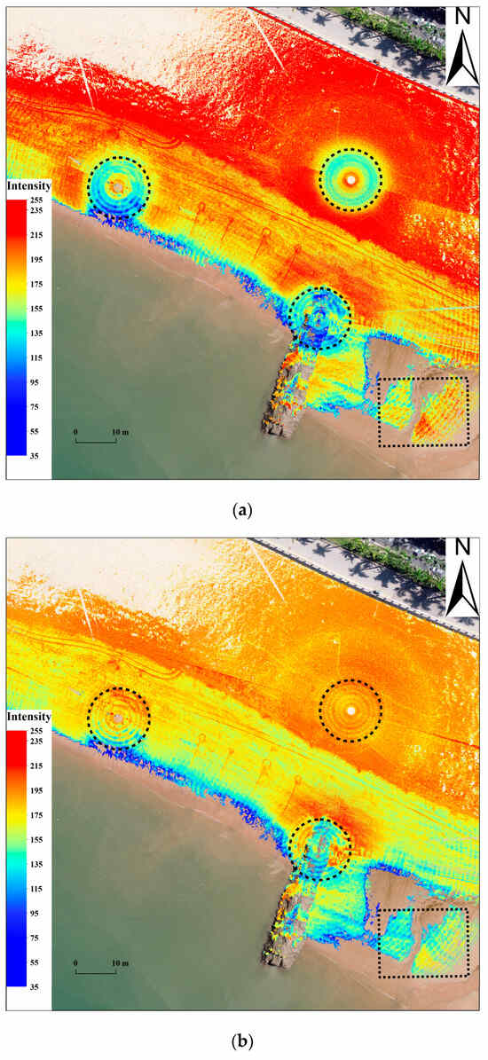
Figure 5.
(a) Original intensity distribution. (b) Corrected intensity distribution.
Figure 5b presents the intensity distribution after correction using the BP network. The intensity correction effectively eliminated the uneven intensity variations caused by distance and incidence angle effects. Compared to the original intensity, the corrected intensity distribution is more uniform and accurately reflects the surface characteristics of the objects. Both the anomalous low-intensity and high-intensity reflections were successfully eliminated. The backshore area of the beach displays a uniform orange color, as the original intensity under the conditions of and ds = 8 m yielded a mean intensity of 185.23, corresponding to an orange color on the scale. Additionally, due to the drainage channel obstructing the longitudinal transport of windblown sand along the coastline, some dry sand has accumulated in this area, resulting in the persistence of a high-intensity reflection region above the drainage channel.
4.2. Sediment Grain Size and Distribution Characteristics
Based on average grain size, the 40 field-collected samples were classified into five categories: fine sand (0.001–0.500 mm), medium sand (0.501–1.000 mm), medium–coarse sand (1.001–1.500 mm), coarse sand (1.501–2.000 mm), and gravel (2.001–2.500 mm).
Figure 6a illustrates the spatial distribution of the average grain size of the 40 samples. On the beach foreshore, particularly near the waterline where direct wave action occurs, the strong wave action causes the separation of sand particles of different grain sizes according to their weights and settling velocities. Gravel and most coarse sand samples are concentrated near the waterline. As beach elevation increases, sediment grain size gradually decreases, and lighter sand particles are transported farther away. Under the influence of wind, the sediment on the beach backshore is smaller in grain size and relatively uniformly distributed, with all fine sand samples concentrated near the beach berm.
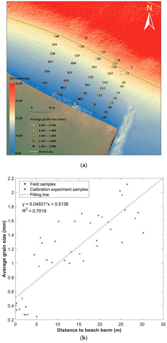
Figure 6.
(a) Characteristics of sediment grain size distribution. (b) Sediment average grain size vs. distance from sampling point to beach berm.
The distance from each sampling point to the beach berm was calculated, and the relationship between average grain size and the distance is shown in Figure 6b. A strong linear relationship (R2 = 0.70) is observed between average grain size and the distance to the beach berm. Specifically, the farther the distance from the beach berm, the larger the grain size of the sediment due to the sorting effects of waves and wind. This finding is consistent with the conclusions drawn by Zheng [26] in this study site.
4.3. Feature Parameters
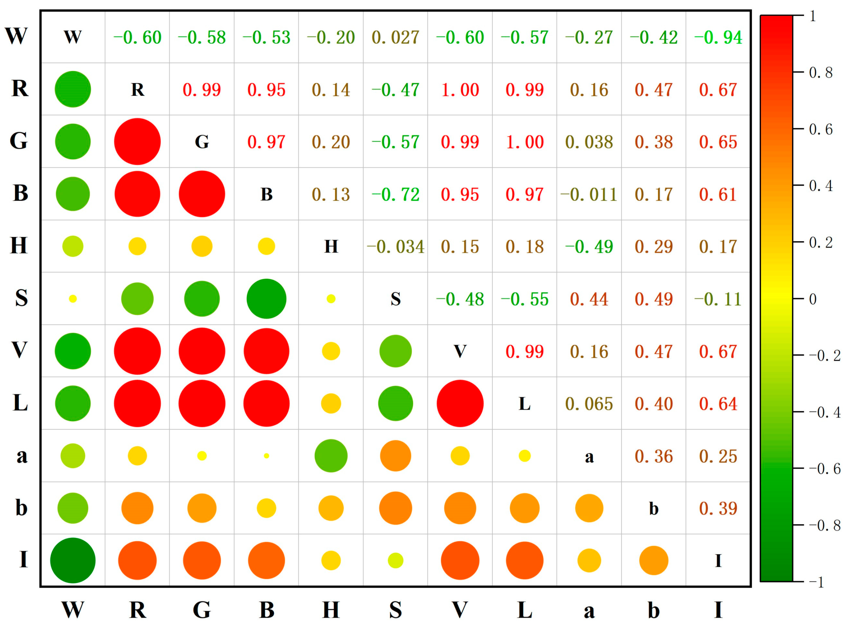
Figure 7 displays the Pearson correlation coefficient matrix between ten feature parameters (color parameters R, G, B, H, S, V, L, a, b, and intensity parameter I) and moisture content W. Among all of the color parameters, those related to brightness exhibit a strong negative correlation with moisture, indicating significant potential for predicting moisture based on color information, with correlation coefficients of −0.60 (R), −0.58 (G), −0.53 (B), −0.60 (V), and −0.57 (L). Moreover, these brightness parameters demonstrate a very strong positive correlation among themselves, with correlation coefficients ranging from 0.95 to 1.00, which suggests consistency in brightness variations across different color spaces. The intensity I shows a very strong negative correlation with moisture, with a correlation coefficient of −0.94, indicating that near-infrared laser responses to moisture changes are highly sensitive. Notably, there is also a strong positive correlation between the intensity and brightness parameters (with coefficients above 0.6), suggesting similar response trends to moisture changes between the near-infrared and visible light bands. To reduce data redundancy, the intensity I and the brightness parameter V, which show the strongest correlation with moisture variation, are ultimately selected as predictor variables.
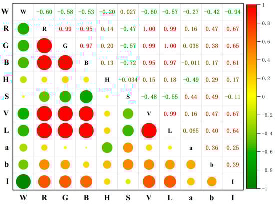
Figure 7.
Correlation coefficient matrix between the feature parameters and moisture content.
4.4. Moisture Estimation
The moisture prediction model trained using the BP network displayed excellent performance. A total of 168 sample data points were used for model training and validation, with 118 samples in the training set and 50 samples in the testing set. The model achieved an RMSE of 1.47 and an of 0.98 on the training set and an RMSE of 1.85 and an of 0.97 on the testing set. In addition, during the modeling process, three machine learning methods were compared: the BP network, SVM (support vector machine), and RF (random forest). The BP network yielded the best results. To maintain the focus of this paper on the advantages of the integrated model, the modeling results of the three machine learning methods were not presented, but instead emphasized the superiority of the integrated model over single-source models (in Section 5.3). The BSM map obtained from the model is shown in Figure 8.
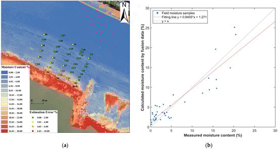
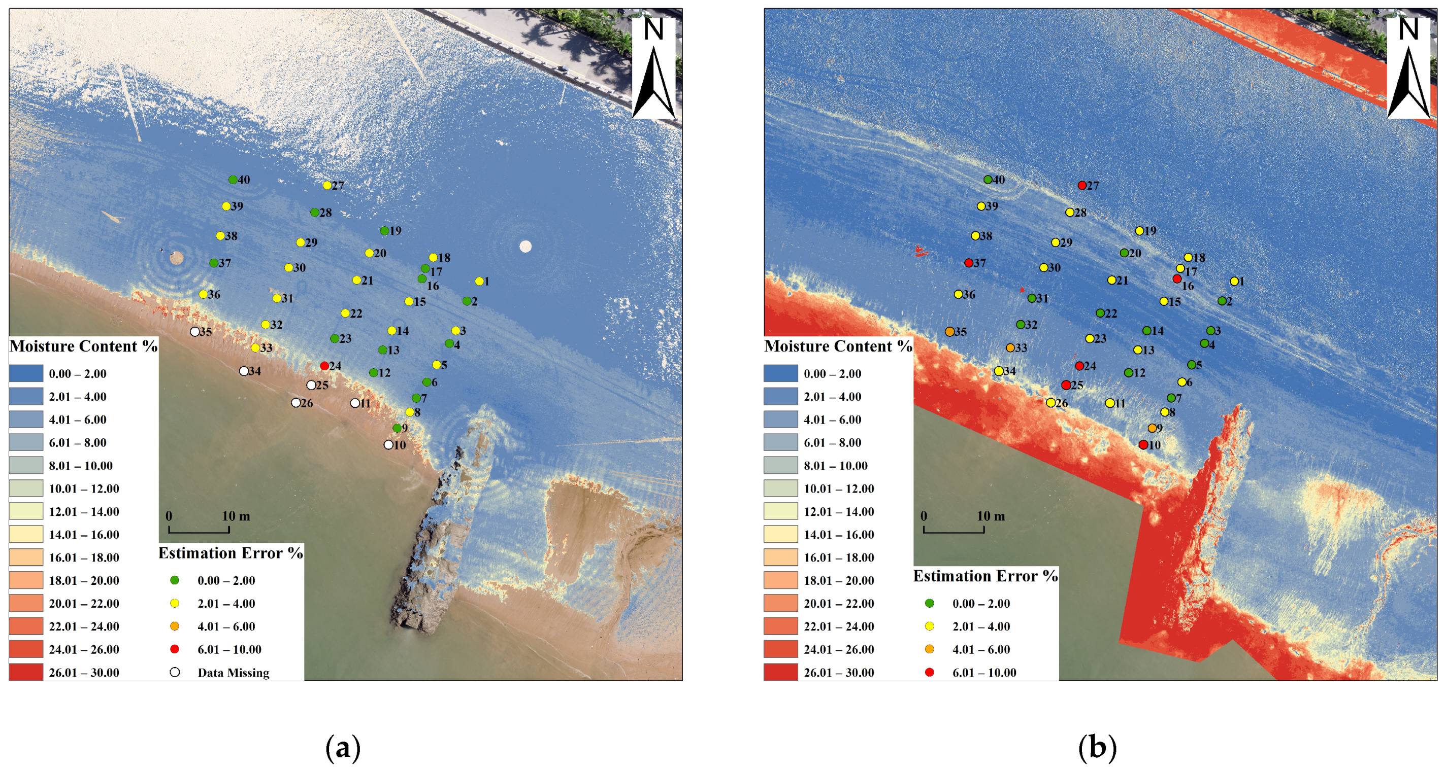
Figure 8.
(a) Distribution of beach surface moisture and estimation errors. (b) Measured moisture of the samples vs. estimated moisture of the samples.
Figure 8a presents the spatial distribution of BSM and the estimation errors. Moisture is represented by a color gradient covering a range from 0% to 30%: deep blue indicates low moisture areas (0–2%), while orange to red indicates high moisture areas (24–30%). The distribution of surface moisture exhibits significant spatial variation, with low-moisture regions concentrated in the backshore area. This area is not affected by wave action and is exposed to intense sunlight, which promotes evaporation and creates dry, sandy conditions. High-moisture regions are concentrated near the waterline in the foreshore area and some low-lying areas, where moisture content is nearly saturated due to tidal action. In the southeastern part of the study site, two low-lying zones show surface water and develop tidal channels that facilitate water transport. An anomalous high-moisture area appears in the northeast of the image. Comparison with the orthophoto of the study site (Figure 1) shows that this region is near urban roads, which lack intensity data, and the shading from trees reduces image brightness and interferes with the moisture estimation results.
Different colored points are utilized to mark the error ranges in Figure 8a: red indicates sampling points with estimation errors exceeding 6%, orange indicates errors between 4% and 6%, yellow indicates errors between 2% and 4%, and green indicates errors within 2%. Regions with higher estimation errors are concentrated near the waterline, where moisture changes are dramatically. There is one sampling point with an error exceeding 6% and three points with errors between 4% and 6%. In medium- to low-moisture regions, the estimation demonstrates relatively high accuracy, with errors at most sampling points within 2%. Among the 40 sampling points, the minimum error is 0.06%, the maximum error is 6.14%, and the RMSE is 2.63%.
Figure 8b uses a scatter plot to compare the moisture estimated with the fusion model with the moisture measured by gravimetric methods. In low-moisture regions, the estimation results are closer to the measured values, indicating that the fusion model has good applicability. In high-moisture regions, the data are more dispersed, with some exhibiting significant estimation errors. The slope of the fitted line approaches 1, suggesting that the estimation model can effectively estimate the trends in moisture changes.
5. Discussion
5.1. Geometric Effect Correction of Original Intensity
Figure 5 presents the overall intensity correction results for the study site. To better illustrate the impact of geometric effects on the original intensity, a strip of the point cloud measuring 58 m in length and 0.2 m in width, as shown in Figure 1, is selected to show more detail.
Figure 9a shows the variation in original intensity with scanning distance. Due to the brightness suppressor within the TLS for close-range measurements, the distance effect on intensity is quite complex [27]. Within 12 m, the intensity shows a sharp decrease (from 2 to 5 m) followed by a sharp increase (from 5 to 12 m). This phenomenon results in an anomalous circular low-reflectance region near the center of measurement station, as seen in Figure 5a. When the distance exceeds 12 m, the overall intensity of the point cloud gradually declines. However, at distances beyond 40 m, a slight but unusual increase is observed, which is reflected in the high reflectance region within the black rectangle in Figure 5a. This anomalous phenomenon may be attributed to the fact that, at long scanning distances, only the surface of sand ripples facing the scanner can return the laser beams, resulting in lower incidence angles that partially compensate for the intensity. Figure 9b illustrates the relationship between the corrected intensity and distance. Compared to the original intensity, the corrected intensity is notably more concentrated, approximating a straight line.
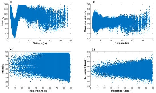
Figure 9.
(a) Relationship between original intensity and distance. (b) Relationship between corrected intensity and distance. (c) Relationship between original intensity and incidence angle. (d) Relationship between corrected intensity and incidence angle.
Figure 9c shows the variation in original intensity with incidence angle. Due to the presence of sand ripples, the incidence angle varies across almost all the range from 0° to 90°. However, under the dual influence of incidence angle and distance effects, the original intensity distribution shows no clear pattern. Figure 9d shows that the variation in corrected intensity with the incidence angle has an approximately isosceles triangular shape. This occurs because the incidence angles of the point cloud rapidly rise to nearly 90° as distance increases. Although the undulations of the beach surface increase the probability of small incidence angles, the incidence angle of the vast majority of the point cloud is still concentrated in the range close to 90°. The value of corrected intensity is very close to the average of the original intensity under the conditions of and m. To quantitatively evaluate the correction effect of the BP model, the coefficient of variation (CV) for the intensity before and after correction is calculated. The results show that the CV of the original intensity is 14.297, while the CV of the corrected intensity is 5.627, indicating a 60.642% reduction. Compared to existing polynomial correction methods, the BP model trained with in situ scanning data can simultaneously correct for incidence angle and distance effects, effectively addressing the complex micro-topographical variations in the beach surface.
5.2. Effect of Grain Size Variation on Feature Parameters
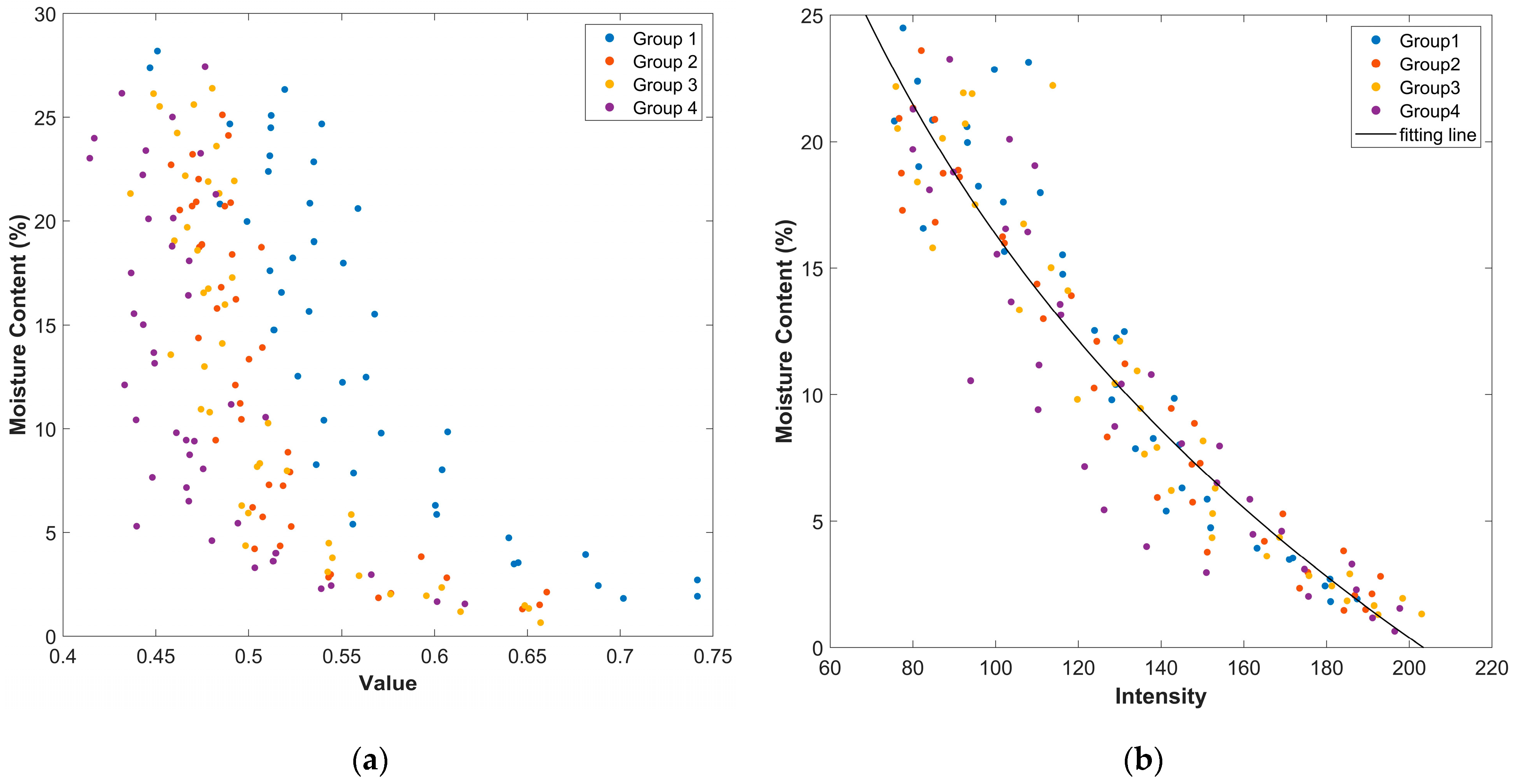
In similar studies, such as those by Jin [28], Tan [29], and Smit [15], the effect of sediment grain size on predictor variables was often overlooked, primarily because these studies choose a study area with a gentle topography (slope angle less than 2°), where the sediment grain size is more concentrated. The study site in this research faces an open sea, where incident wave energy is strong, and the beach slope angle is approximately 6°, resulting in a more complex beach environment. The steep terrain leads to significant variations in grain size of sand, making it essential to consider the effects of grain size variation in the predictive model. To further explore this, the 12 samples from the calibration experiment are categorized into four groups based on average grain size: fine sand (Group 1), medium sand (Group 2), medium–coarse sand (Group 3), and coarse sand (Group 4). The relationships between feature parameters and moisture content under different grain size conditions are illustrated in Figure 10. Sample groups and average grain sizes are detailed in Table 1.
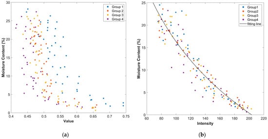
Figure 10.
Relationship between feature parameters and moisture content under different grain size conditions. (a) V (from HSV color space) vs. moisture. (b) Intensity vs. moisture.

Table 1.
Group and average grain size of calibrated experimental samples.
Figure 10a shows the effect of grain size on brightness. When samples are grouped by grain size, the brightness variation within each group becomes more consistent. Under identical moisture content, samples with smaller grain size display significantly higher brightness. This is primarily due to micro-shadows formed by pore spaces between sand grains; larger grains produce larger pores, which increase the shadowed area and thus reduce overall brightness. Therefore, it is crucial to consider the effect of grain size variation on brightness. In contrast, TLS with an active remote sensing approach avoids this problem because it is virtually unaffected by changes in environmental light. Figure 10b indicates that grain size variations have almost no influence on intensity.
5.3. Advantages of Data Fusion
The application of the data fusion methods in this study provides a new approach for obtaining high spatial and temporal resolutions of BSM. In contrast, traditional single-source data inversion methods are limited in accuracy and stability. By comparing the inversion results of the two methods, the role of multi-source data in accuracy improvement can be more clearly understood.
The exponential model developed by Jin [28] is used to complete the intensity-based moisture estimation with the following formula:
where is the corrected intensity and is the moisture. and are two constants determined by the laser wavelength and the sediment properties.
Moisture estimation based on brightness is performed using a BP network, where the correction of brightness is automatically performed by the model:
where is the moisture, is brightness, and is sediment grain size, which is estimated by Equation (10).
The BSM distribution based on intensity is shown in Figure 11a. Due to the installation height of the TLS and the open environment of the beach, frequent interference from pedestrians and moving objects led to many radial data holes. Due to the strong absorption of water to the near-infrared laser, the range of the point cloud acquired by the TLS is limited, with data missing from six sampling points under the tidal flush. A huge data hole at the low-lying part of the beach on the southeast side due to the presence of water on the surface, making it impossible to acquire the tidal gully data on the beach foreshore. Thanks to the advantages of active remote sensing, TLS is minimally affected by environmental light, yielding satisfactory inversion accuracy: among the 34 sampling points, the minimum error is 0.08%, the maximum error is 8.45%, and the RMSE is 2.83%. Eleven sampling points have errors within 2%; however, a significant error exceeding 6% is observed at one sampling point near the waterline.
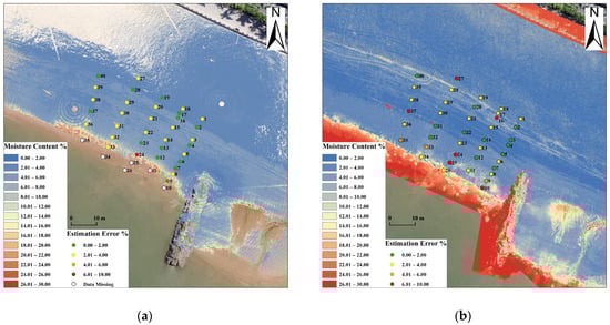
Figure 11.
(a) Distribution of beach surface moisture based on intensity. (b) Distribution of beach surface moisture based on brightness.
The inversion based on the brightness resulted in a complete distribution of the BSM (Figure 11b), yet passive remote sensing is more susceptible to environmental light interference, with shadows constituting a primary error source. The backshore of the beach, where sand is dry and fine, shows countless small sand dens (5–10 cm) formed under tourist foot traffic, with shadows in the centers of these dens appearing as bright yellow micro-areas in the image. The boundary between the dry and wet area exhibits more pronounced inversion errors, with two sampling points showing errors exceeding 6%. This is due to the denser sand composition on the beach foreshore resulting from tidal flushing, which causes significant changes in slope and increases shadowing. In the central region, similar shadow interference resulted in one sampling point within a small sand pit exhibiting an inversion error exceeding 6%. In high-moisture areas, brightness yields more comprehensive inversion results, as evidenced by the complete southeastern beach data, where tidal channels are clearly visible. However, this area also shows the highest inversion errors, with three sampling points showing errors greater than 6% and two points showing errors between 4% and 6%. Although visible light can penetrate the thin water layer, the specular reflection and refraction produced by the water surface introduce non-negligible interference to the image. Overall, the brightness-based moisture inversion achieved better results only in the flat central region of the wet beach, with a minimum error of 0.04%, a maximum error of 13.36%, and an RMSE of 4.23%.
Compared to single-source methods, the fusion of active and passive remote sensing data expands the range of information selection for the model, allowing for the BP network to integrate key features more effectively during adaptive learning and optimizing the error reduction pathway. Compared to Figure 8a, it is evident that the fusion model substantially improves predictive accuracy. In dry beach areas, the inclusion of active remote sensing data largely eliminates shadow interference. In wet beach areas, the collaboration of active and passive remote sensing data provides the model with more comprehensive information, mitigating the influence of grain size variation under the combined effect of intensity and grain size, thus enhancing the model’s robustness and achieving higher inversion accuracy. Notably, in the low-lying areas of the southeastern beach where surface water is present, the inversion results from the fusion model are closer to the actual conditions. Despite the lack of intensity data in this area, the BP network model can recognize high moisture in regions characterized by low brightness, large grain size, and missing intensity data, greatly enhancing the model’s generalization capability.
5.4. Limitations and Future Directions
Although the method proposed in this study demonstrates good results, there are still some limitations, and future research can build upon this work for further improvements. The field data collection was completed within half an hour, during which it was assumed that solar radiation did not experience significant changes. However, during the calibration experiment, the acquisition of digital images lasted for several hours, during which noticeable changes in the illumination occurred. To correct color distortion caused by these illumination variations, a standard gray card and standard color card were employed, providing a basis for the accurate analysis of the color information in the sample images. Nevertheless, specialized instruments for measuring solar radiation were not utilized in this study. The measurement of solar radiation is believed to significantly enhance the model’s performance, especially when considering the impact of external environmental factors on sample moisture. Therefore, future research should focus on enhancing the analysis of environmental factors, such as solar radiation, wind speed, wind direction, and tidal levels. The objective is to incorporate more environmental data into the model and conduct tests for generating time-series moisture maps. This approach would help to more comprehensively capture the effects of environmental factors on moisture variation and further improve the predictive capability of the model.
6. Conclusions
This study combines digital image and LiDAR technology to analyze the effects of sediment grain size variation on image brightness and laser point cloud intensity. It proposes a method for estimating BSM using a BP network that integrates both active and passive remote sensing data. The main conclusions are as follows:
(1) Using in situ scanning data to perform the intensity correction process in a beach environment avoids time-consuming indoor and outdoor calibration procedures while reducing the interference of environmental variables on data consistency. Compared to existing polynomial correction methods, the BP network effectively captures the complex nonlinear relationships between scanning geometry and original intensity, enabling efficient and accurate intensity correction for the complex micro-topography of the beach surface.
(2) Sediment grain size has a significant effect on image brightness, as larger pores between coarse sand particles produce more tiny shadows, which reduce the overall brightness of the image. In contrast, the data acquired through TLS using active remote sensing is largely unaffected by environmental light, meaning that intensity is minimally influenced by variations in sediment grain size.
(3) The moisture prediction model that integrates active and passive remote sensing data effectively expands the range of information selection, allowing for the integration of key features between datasets and eliminating the interference of shadows. Compared to existing studies, the comprehensive utilization of information from three dimensions—brightness, intensity, and grain size—significantly enhances the robustness of the fusion model and broadens its applicability. The fusion model provides accurate moisture predictions on complex beaches with steep slopes (approximately 6°) and significant grain size variations, achieving an RMSE of only 2.63% across all 40 samples.
Supplementary Materials
The following supporting information can be downloaded at: https://www.mdpi.com/article/10.3390/rs17030522/s1.
Author Contributions
All authors contributed to the results and discussion of the manuscript. J.Z. proposed the method and wrote the paper; J.Z. conceived and designed the experiments, J.Z., F.Y. and P.S. performed the experiments; J.Z. and K.T. analyzed the data; F.H. provided materials and analytical tools. All authors have read and agreed to the published version of the manuscript.
Funding
This work was funded by the National Natural Science Foundation of China (Grant 42171425, Grant 42471473), the International Joint Laboratory of Estuarine and Coastal Research, Shanghai (Grant 21230750600), the Science and Technology Commission of Shanghai Municipality (Grant 22ZR1420900), and the Key Laboratory of Geographic Information Science (Ministry of Education), East China Normal University (Grant KLGIS2024A02).
Data Availability Statement
The original contributions presented in this study are included in the article and Supplementary Material. Further inquiries can be directed to the corresponding author.
Acknowledgments
The authors wish to thank Rongcan Shi (Third Institute of Oceanography, Ministry of Natural Resources, China) for their logistical and technical assistance during the field experiments.
Conflicts of Interest
The authors declare no conflicts of interest.
References
- de Schipper, M.A.; Ludka, B.C.; Raubenheimer, B.; Luijendijk, A.P.; Schlacher, T.A. Beach nourishment has complex implications for the future of sandy shores. Nat. Rev. Earth Environ. 2021, 2, 70–84. [Google Scholar] [CrossRef]
- Lopez, O.M.; Hegy, M.C.; Missimer, T.M. Statistical comparisons of grain size characteristics, hydraulic conductivity, and porosity of barchan desert dunes to coastal dunes. Aeolian Res. 2020, 43, 100576. [Google Scholar] [CrossRef]
- van Westen, B.; de Vries, S.; Cohn, N.; van Ijzendoorn, C.; Strypsteen, G.; Hallin, C. AeoLiS: Numerical modelling of coastal dunes and aeolian landform development for real-world applications. Environ. Model. Softw. 2024, 179, 106093. [Google Scholar] [CrossRef]
- Davidson-Arnott, R.G.D.; Yang, Y.; Ollerhead, J.; Hesp, P.A.; Walker, I.J. The effects of surface moisture on aeolian sediment transport threshold and mass flux on a beach. Earth Surf. Process. Landf. 2008, 33, 55–74. [Google Scholar] [CrossRef]
- Edwards, B.L.; Namikas, S.L. Small-scale variability in surface moisture on a fine-grained beach: Implications for modeling aeolian transport. Earth Surf. Process. Landf. 2009, 34, 1333–1338. [Google Scholar] [CrossRef]
- Yang, X.; Yu, Y.; Li, M. Estimating soil moisture content using laboratory spectral data. J. For. Res. 2019, 30, 1073–1080. [Google Scholar] [CrossRef]
- Philpot, W. Spectral Reflectance of Wetted Soils. In Proceedings of the Art, Science and Applications of Reflectance Spectroscopy (ASARS), Boulder, CO, USA, 23–25 February 2010. [Google Scholar]
- Persson, M. Estimating Surface Soil Moisture from Soil Color Using Image Analysis. Vadose Zone J. 2005, 4, 1119–1122. [Google Scholar] [CrossRef]
- Liu, G.; Tian, S.; Xu, G.; Zhang, C.; Cai, M. Combination of effective color information and machine learning for rapid prediction of soil water content. J. Rock Mech. Geotech. Eng. 2023, 15, 2441–2457. [Google Scholar] [CrossRef]
- Darke, I.; Davidson-Arnott, R.; Ollerhead, J. Measurement of Beach Surface Moisture Using Surface Brightness. J. Coast. Res. 2009, 25, 147–256. [Google Scholar] [CrossRef]
- Delgado-Fernandez, I. Meso-scale modelling of aeolian sediment input to coastal dunes. Geomorphology 2011, 130, 230–243. [Google Scholar] [CrossRef]
- Delgado-Fernandez, I.; Davidson-Arnott, R.; Ollerhead, J. Application of a Remote Sensing Technique to the Study of Coastal Dunes. J. Coast. Res. 2009, 25, 1160–1167. [Google Scholar] [CrossRef]
- Jin, J.; De Sloover, L.; Verbeurgt, J.; Stal, C.; Deruyter, G.; Montreuil, A.-L.; De Maeyer, P.; De Wulf, A. Measuring Surface Moisture on a Sandy Beach based on Corrected Intensity Data of a Mobile Terrestrial LiDAR. Remote Sens. 2020, 12, 209. [Google Scholar] [CrossRef]
- Nield, J.M.; King, J.; Jacobs, B. Detecting surface moisture in aeolian environments using terrestrial laser scanning. Aeolian Res. 2014, 12, 9–17. [Google Scholar] [CrossRef]
- Smit, Y.; Ruessink, G.; Brakenhoff, L.B.; Donker, J.J.A. Measuring spatial and temporal variation in surface moisture on a coastal beach with a near-infrared terrestrial laser scanner. Aeolian Res. 2018, 31, 19–27. [Google Scholar] [CrossRef]
- Elsherif, A.; Gaulton, R.; Mills, J. Four Dimensional Mapping of Vegetation Moisture Content Using Dual-Wavelength Terrestrial Laser Scanning. Remote Sens. 2019, 11, 2311. [Google Scholar] [CrossRef]
- Junttila, S.; Hölttä, T.; Puttonen, E.; Katoh, M.; Vastaranta, M.; Kaartinen, H.; Holopainen, M.; Hyyppä, H. Terrestrial laser scanning intensity captures diurnal variation in leaf water potential. Remote Sens. Environ. 2021, 255, 112274. [Google Scholar] [CrossRef]
- Junttila, S.; Sugano, J.; Vastaranta, M.; Linnakoski, R.; Kaartinen, H.; Kukko, A.; Holopainen, M.; Hyyppä, H.; Hyyppä, J. Can Leaf Water Content Be Estimated Using Multispectral Terrestrial Laser Scanning? A Case Study with Norway Spruce Seedlings. Front. Plant Sci. 2018, 9, 299. [Google Scholar] [CrossRef]
- Fang, W.; Huang, X.; Zhang, F.; Li, D. Intensity Correction of Terrestrial Laser Scanning Data by Estimating Laser Transmission Function. IEEE Trans. Geosci. Remote Sens. 2015, 53, 942–951. [Google Scholar] [CrossRef]
- Sanchiz-Viel, N.; Bretagne, E.; Mouaddib, E.M.; Dassonvalle, P. Radiometric correction of laser scanning intensity data applied for terrestrial laser scanning. ISPRS J. Photogramm. Remote Sens. 2021, 172, 1–16. [Google Scholar] [CrossRef]
- Tan, K.; Cheng, X. Intensity data correction based on incidence angle and distance for terrestrial laser scanner. J. Appl. Remote Sens. 2015, 9, 094094. [Google Scholar] [CrossRef]
- Chen, B.; Yang, Y.; Wen, H.; Ruan, H.; Zhou, Z.; Luo, K.; Zhong, F. High-resolution monitoring of beach topography and its change using unmanned aerial vehicle imagery. Ocean Coast. Manag. 2018, 160, 103–116. [Google Scholar] [CrossRef]
- Pan, Y.; Flindt, M.; Schneider-Kamp, P.; Holmer, M. Beach wrack mapping using unmanned aerial vehicles for coastal environmental management. Ocean Coast. Manag. 2021, 213, 105843. [Google Scholar] [CrossRef]
- Nolet, C.; Poortinga, A.; Roosjen, P.; Bartholomeus, H.; Ruessink, G. Measuring and Modeling the Effect of Surface Moisture on the Spectral Reflectance of Coastal Beach Sand. PLoS ONE 2014, 9, e112151. [Google Scholar] [CrossRef]
- Zhang, C.; Liu, J.; Yang, J. Studies on muddy and consolidating process at Silver Beach in Beihai. Mar. Forecast. 2017, 34, 83–88. [Google Scholar] [CrossRef]
- Zheng, W.; Cao, C.; Cai, F.; Qi, H.; He, Y.; Li, Y.; Liu, G.; Zhao, S. Responses of sediment grain size to seasonal variation of Baicheng beach morphology in Xiamen, China. J. Appl. Oceanogr. 2024, 43, 533–544. [Google Scholar] [CrossRef]
- Höfle, B.; Pfeifer, N. Correction of laser scanning intensity data: Data and model-driven approaches. ISPRS J. Photogramm. Remote Sens. 2007, 62, 415–433. [Google Scholar] [CrossRef]
- Jin, J.; Verbeurgt, J.; De Sloover, L.; Stal, C.; Deruyter, G.; Montreuil, A.-L.; Vos, S.; De Maeyer, P.; De Wulf, A. Monitoring spatiotemporal variation in beach surface moisture using a long-range terrestrial laser scanner. ISPRS J. Photogramm. Remote Sens. 2021, 173, 195–208. [Google Scholar] [CrossRef]
- Tan, K.; Chen, J.; Zhang, W.; Liu, K.; Tao, P.; Cheng, X. Estimation of soil surface water contents for intertidal mudflats using a near-infrared long-range terrestrial laser scanner. ISPRS J. Photogramm. Remote Sens. 2020, 159, 129–139. [Google Scholar] [CrossRef]


Disclaimer/Publisher’s Note: The statements, opinions and data contained in all publications are solely those of the individual author(s) and contributor(s) and not of MDPI and/or the editor(s). MDPI and/or the editor(s) disclaim responsibility for any injury to people or property resulting from any ideas, methods, instructions or products referred to in the content. |
© 2025 by the authors. Licensee MDPI, Basel, Switzerland. This article is an open access article distributed under the terms and conditions of the Creative Commons Attribution (CC BY) license (https://creativecommons.org/licenses/by/4.0/).