Inter-Annual Variability of Peatland Vegetation Captured Using Phenocam- and UAV Imagery

Abstract

Plant phenology is an important driver of inter-annual variability in peatland carbon uptake. However, the use of traditional phenology datasets (e.g., manual surveys, satellite remote sensing) to quantify this link is hampered by their limited spatial and temporal coverage. This study examined the use of phenology cameras (phenocams) and uncrewed aerial vehicles (UAVs) for monitoring phenology in a Scottish temperate peatland. Data were collected at the site over multiple growing seasons using a UAV platform fitted with a multispectral Parrot Sequoia camera. We found that greenness indices calculated using data from both platforms were in strong agreement with each other, and exhibited strong correlations with rates of gross primary production (GPP) at the site. Greenness maps generated with the UAV data were combined with fine-scale vegetation classifications, and highlighted the variable sensitivity of different plant species to dry spells over the study period. While a lack of suitable weather conditions for surveying limited the UAV data temporally, the phenocam provided a near-continuous record of phenology. The latter revealed substantial temporal variability in the relationship between canopy greenness and peatland GPP, which although strong over the growing season as a whole (r_s = 0.88, p < 0.01), was statistically insignificant during the peak growing season.

1. Introduction

1.1. Vegetation Drives Seasonal Carbon Dynamics

Terrestrial ecosystems and their vegetation are key components of the global carbon cycle and an important control on its dynamics [1]. Indeed, the seasonal greening of vegetation in the northern hemisphere and its photosynthesis are large enough to be observed in global atmospheric carbon-dioxide (CO₂) concentrations [2,3]. This plant phenology describes the timing of lifecycle events, including spring green-up, flowering, and autumn senescence [4]. These events are regulated by internal biological mechanisms and tightly coupled to a range of environmental drivers, which makes them sensitive to change [5]. Global shifts in phenology have been observed since the mid-20th Century in response to climate change [6,7,8,9,10], with earlier spring growth and later senescence [11,12] leading to a longer growing season [8,13,14]. That said, predicted future increases in the frequency and severity of extreme weather events (e.g., drought) [15] may limit the length of the vegetation period [16,17]. In either case, future phenological shifts are expected to have large implications for the global carbon cycle [5,18,19].

1.2. Carbon Fluxes in Northern Peatlands and Responses to Climate Change

Northern peatlands are particularly vulnerable to change. These ecosystems constitute a globally significant carbon sink of around 400–600 Pg C [20,21], and have experienced favourable environmental conditions since the Holocene (e.g., a cool, wet climate and high water-table), inhibiting the decomposition of organic matter [22,23]. Under scenarios of future climate change, however, northern latitudes are expected to experience above-average rates of warming, alongside more frequent and extreme weather events [15,24,25]. Such changes risk destabilising peatland carbon stocks by accelerating rates of decomposition [26]. Although an earlier start to the growing season in response to rising temperature would (in principle) increase the number of days where an ecosystem can assimilate carbon by photosynthesis [27,28,29], the complex feedbacks between weather, phenology, and ecosystem functioning make it difficult to predict the overall impact of phenological shifts on peatland carbon cycle dynamics [5,19,30,31].

The Net Ecosystem Exchange of CO₂ (NEE) in a peatland is the difference between the amount of CO₂ released by ecosystem respiration (R_eco) and that assimilated by photosynthesis (i.e., Gross Primary Production, GPP). Over short (daily, seasonal, inter-annual) timescales, peatlands display a strong variability in carbon uptake, and a number of sites have demonstrated the ability to switch from functioning as a net sink for CO₂, to a net source between years. This variability has often been attributed to weather events such as heatwaves and altered precipitation patterns [17,32,33], which can affect both plant physiology (e.g., by drought-induced stress) and phenology (e.g., if drought stress induces early senescence). Such research, however, has to date been limited and is hampered by a lack of high-quality, long-term phenology datasets.

1.3. Phenological Monitoring

1.3.1. Manual Surveys and Remote Sensing

In terms of monitoring, the inaccessible and remote nature of many peatland sites means that traditional, manual observations of phenology are rare. As an alternative, studies often examine (near) remote-sensing phenology; either using data from automated camera setups (i.e., phenocams [34,35,36]), or from satellite imagery [37,38,39]. While phenocams provide near-continuous ‘true-colour’ imagery over a fixed field of view in the red, green, and blue bands (RGB), satellites can exploit data from multispectral (containing as few as 3–4 bands) or hyperspectral sensors (containing hundreds of sampled bands) and provide spectrally rich, calibrated data.

Remote sensing studies commonly employ vegetation indices (VIs) as a proxy for plant phenology and physiology. These are combinations of bands known to relate to vegetation structure (e.g., biomass, leaf area), vegetation biogeochemistry (e.g., water content, pigments, chlorophyll), and physiological status (e.g., light use efficiency, stress marked by changes in pigmentation) [40]. VI time-series can be used to estimate the timing of phenological events (e.g., leaf out, flowering date, senescence) (e.g., ref. [41]). Furthermore, at sites with available greenhouse gas measurements, these time-series data can be used to examine: (i) the response of vegetation to weather events (e.g., ref. [42]); and (ii) the impact of phenology on ecosystem functioning and land–atmosphere exchange (termed flux hereafter) of CO₂ [38,43,44].

1.3.2. Limitations of Current Remote Sensing Approaches

Phenology metrics derived using remote sensing are sensitive to the resolution of data employed [45,46,47,48], which is an inherent problem [49,50]. At the ground level, phenology is strongly heterogeneous, both spatially and temporally. Field measurements in a deciduous forest, for example, found that the onset of greening varied by as much as 2 weeks over distances <500 m, despite stands having similar composition, age and structural characteristics [51]. Such fine-scale heterogeneity (e.g., differences due to micro-topography or species type) is not captured by the relative coarseness of satellite data pixels, which commonly employ spatial resolutions > 30 m. This ‘coarse’ spatial resolution can be problematic as it masks a large amount of heterogeneity and pixels contain mixed spectral signals [47]. As such, satellite data are often not comparable with the plot scale (0.1–1 m²) at which many flux measurements are conducted, which makes it difficult to directly compare datasets. The temporal coverage of phenology datasets is also important. For example, differences in the temporal resolution of satellite data products (e.g., comparing the MODIS 8 day and twice daily vegetation index timeseries) were found to cause a discrepancy of over 30 days in the timing of inferred phenological stages in a deciduous forest [52].

Phenocam data, although advantageous in their high temporal resolution, are spatially limited. The majority of peatland phenocam studies examine greenness averaged across a single region of interest (ROI), spanning multiple species with varying phenology; whereas few have examined phenology at the community or plot level, and related this to photosynthetic uptake of CO₂ [53,54]. Furthermore, phenocams are consumer-grade cameras, and hence the acquired images are neither spatially referenced nor spectrally calibrated. As such, phenocam-derived phenology metrics are hard to scale and compare, for example with satellite data.

1.3.3. State of the Art: UAVs for Phenological Monitoring

An alternative and more novel approach for monitoring phenology involves the use of Uncrewed Aerial Vehicles (UAVs). UAVs equipped with RGB, multispectral, or hyperspectral sensors can be used to collect data across a range of spatial and temporal scales, and have much potential in studies examining the heterogeneity of peatland environments and their phenology [55,56,57]. UAV data can be spectrally calibrated and geo-referenced over a defined survey area, which facilitates their comparison with measurements at the plot- and ecosystem scale (100–10⁶ m²), as well as with satellite data. Furthermore, UAV platforms can collect data at an ultra-high spatial resolution, with ground sampling distances (GSDs, i.e., the distance on the ground covered by each image pixel) in the order of centimetres. As such, UAVs have become a valuable tool for tracking fine-scale heterogeneity in greening, e.g., of individual tree crowns [56,58,59] and agricultural crops [60]. However, detailed time-series of UAV data in peatland environments are rare due to their structural complexity and pronounced spatial heterogeneity. In a recent study of a Finnish peatland, Räsänen et al. [61] examined a combination of hyperspectral UAV data and ground-based measurements for detecting patterns in vegetation. The authors demonstrated the potential of UAVs for detecting seasonal trends and fine-scale spatial variability in structural characteristics such as leaf area and biomass. Assmann et al. [62] used a multispectral UAV platform to examine changes in greenness in a tundra environment, finding that a GSD of 0.5 m was able to capture the variability in dominant vegetation types. By spatially aggregating UAV image pixels (5-cm GSD), the authors reported that as much as 60% of seasonal variability in greenness was lost at the spatial resolution of the employed satellite datasets (e.g., Landsat, 30 m; Sentinel-2, 10 m), highlighting the benefits of UAV-based monitoring over satellite data.

Inter-comparison studies employing data across multiple spatial and temporal scales are key to improving our understanding of vegetation phenology and its impact on CO₂ exchange [56,63,64,65]. In boreal peatland ecosystems, for example, Linkosalmi et al. [53], found a strong agreement between phenocam- and satellite-derived VIs. The authors found that while seasonal changes in greenness were closely correlated with peatland GPP, short-term variability in GPP could only be explained by phenocam-derived greenness during certain periods. Multi-scale comparison studies incorporating UAV data are rare, although a study by Berra et al. [56] compared ground-, UAV-, and satellite-based observations of phenology at a mixed woodland. They found that fine-scale UAV data were able to track canopy phenology of individual trees, whereas satellite-derived datasets were related to phenological dynamics at the ecosystem scale.

1.4. Research Outline and Aims

Our study aims to improve understanding of the role of phenology on CO₂ flux across a range of spatial and temporal scales. For this purpose, we examined the use of phenocam imagery and multispectral UAV data to track vegetation phenology over multiple growing seasons in a temperate Scottish peatland. We examined the use of both phenocam- and UAV-derived greenness metrics as a proxy for photosynthetic CO₂ uptake. Finally, in a unique approach, we combined centimetre-resolution UAV data with a vegetation classification map to examine species-level changes in greenness in response to weather anomalies experienced at the site.

2. Materials and Methods

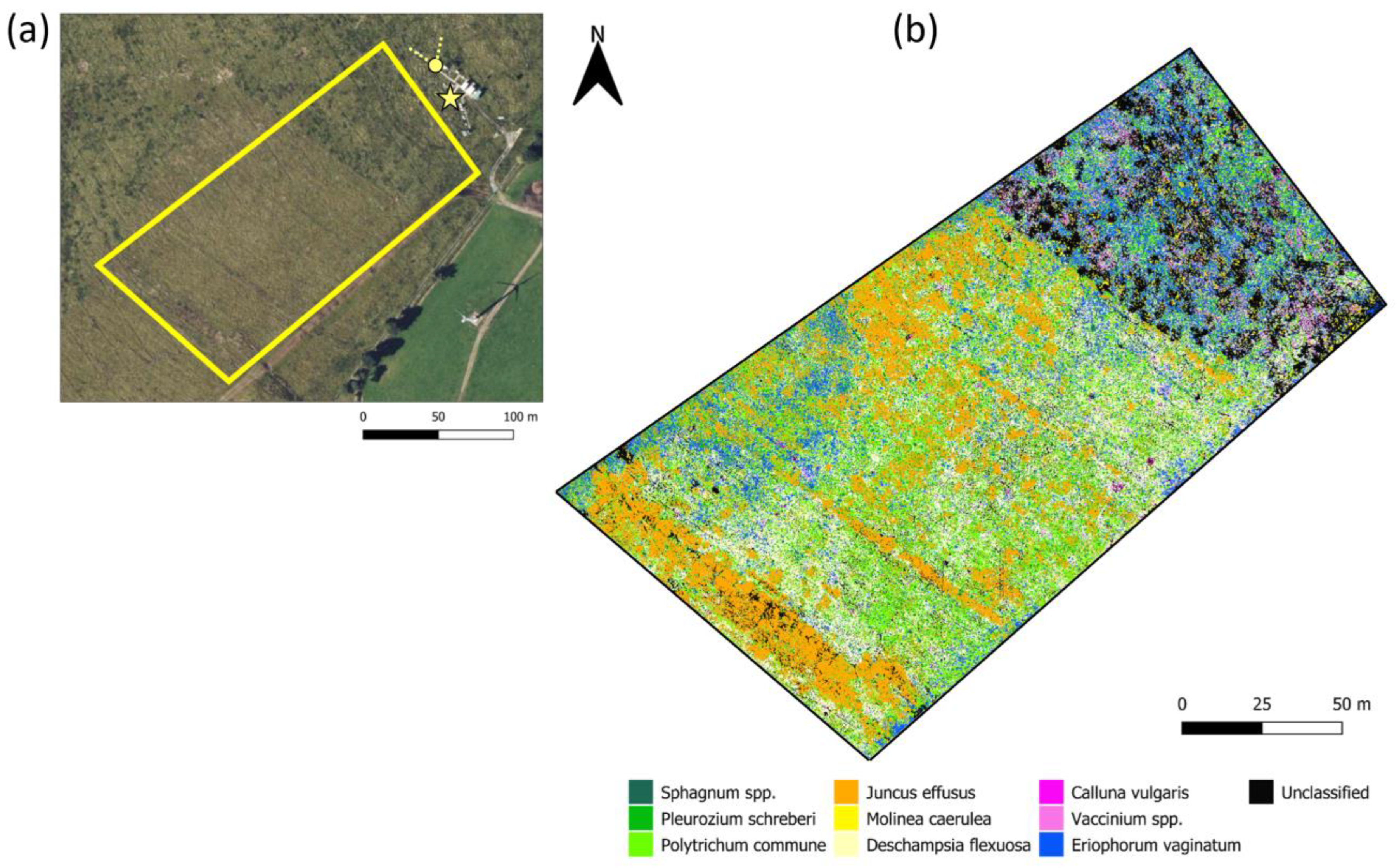
2.1. Study Area

Auchencorth Moss is a low-lying ombrotrophic peatland, located in southeast Scotland (55°47′33 N, 3°14′37 W; 267 m a.s.l.). Shown in Figure 1, the site covers an area of around 1000 ha, with extensive homogeneous fetch over blanket bog to the south, west, and north. A series of regular, parallel ditches indicate the area was historically drained (>100 years ago), although these are now overgrown with vegetation. The peatland has naturally returned to a rewetted state and is currently used for low-density sheep grazing (<1 ha⁻¹). The main soil types in the catchment area are histosols (85%), followed by gleysols (9%), humic gleysols (3%) and cambisols (3%), although the presence of these soil types is mainly limited towards the catchment edge [66].

The site experiences a temperate maritime climate (Köppen–Geiger classification, Ref. [67]), consisting of mild winters with infrequent snowfall, and warm temperatures during the summer months. Mean annual air temperature and total annual precipitation at the site are 7.7 ± 0.6 °C and 963 ± 176 mm, respectively (all values for the period 2002–2017 unless otherwise stated). The site is generally wet, with average daily water table depth (WTD) close to the surface (WTD = 0.9 ± 2.6 cm since recording started in 2007, where positive values indicate a water-table below the surface). WTD displays seasonal variability, and daily values over the long-term measurement record range from −8.5 to 50 cm, reaching their lowest during summer months. The site has mostly functioned as a net sink for CO₂ since 2002, with an average annual uptake of −1.16 ± 0.8 mol CO₂ m⁻² y⁻¹ (for 2002–2023; range: −9.88 ± 2.9 mol CO₂ m⁻² y⁻¹ to 6.14 ± 2.5 mol CO₂ m⁻² y⁻¹).

A regular hummock-hollow micro-topography characterises Auchencorth Moss, typical of many peatlands. Raised hummocks (ca. 40 cm diameter, 30 cm tall) are dominated by a mixture of pleurocarpous mosses (e.g., Pleurozium schreberi, Rhytidiadelphus squarrosus, Hylocomium splendens) and vascular vegetation (e.g., Eriophorum vaginatum, Deschampsia flexuosa, Juncus effusus), whereas hollow microsites (due to their lower elevation) are generally wetter, dominated by mosses (e.g., Sphagnum spp., Polytrichum commune) and some grasses.

2.2. UAV Data

2.2.1. Data Collection

UAV surveys were conducted over the 2018, 2019 and 2021 growing seasons (April to October) using a custom-built hexacopter developed by the Airborne Research and Innovation facility (University of Edinburgh), based around the Tarot T680 Pro airframe (Wenzhou Tarot Aviation Technology Co., Wenzhou, China) and a 3DR Pixhawk flight controller running ArduPilot firmware (http://www.ardupilot.org, accessed on 15 October 2017). Due to the global pandemic, no sampling was conducted during 2020. Repeat surveys were flown over a 0.05 km² area (see Figure 1), following a fixed flight path with 80% front- and side-lap, programmed using the Mission Planner software (v1.3.5, ArduPilot). Analysis of historical data identified this as the dominant source area for CO₂ fluxes measured at the site, allowing for a comparison of greenness and flux data.

Surveying was limited to days with specific meteorological conditions in an attempt to collect the best-quality imagery [68,69]. These were days with: (i) low wind-speeds (<10 m s⁻¹) to reduce blur and limit movement of the vegetation canopy; and (ii) stable meteorological conditions (e.g., consistent clear skies or overcast conditions) to reduce effects of variable scene illumination. Furthermore, all UAV surveys were conducted within 2 h of solar noon to limit the impact of shadow on the collected imagery.

Figure 1. Study site overview. Panel (a) shows an aerial image of Auchencorth Moss alongside the UAV survey area (yellow box), with the location of the meteorological measurement mast (star), flux measurement tower and phenocam (circle) as well as its field of view (dotted lines) shown for reference. Panel (b) shows the employed species-level classification of the UAV survey area (see [70]). Map tile (a) by the Microsoft^® Bing™ Maps Platform API (Microsoft Corporation, Redmond, WA, USA), under General Rights and Restrictions for Prints. Data by OpenStreetMap, under ODbL.

Figure 1. Study site overview. Panel (a) shows an aerial image of Auchencorth Moss alongside the UAV survey area (yellow box), with the location of the meteorological measurement mast (star), flux measurement tower and phenocam (circle) as well as its field of view (dotted lines) shown for reference. Panel (b) shows the employed species-level classification of the UAV survey area (see [70]). Map tile (a) by the Microsoft^® Bing™ Maps Platform API (Microsoft Corporation, Redmond, WA, USA), under General Rights and Restrictions for Prints. Data by OpenStreetMap, under ODbL.

Multispectral data were collected using a Parrot Sequoia camera (Parrot Drones SAS, Paris, France) mounted on the UAV to acquire images in the green, red, red-edge, and near infra-red (NIR) bands (see

Table 1. Spectral information for the four Parrot Sequoia bands.

Band Name	Central Band Wavelength ± Width (nm)
Green	550 ± 40
Red	660 ± 40
Red-Edge	735 ± 10
Near Infra-Red	790 ± 40

). This camera consists of two components: (i) a downward-facing lens, which captures imagery of the surveyed scene; and (ii) a skyward-facing incident light sensor (Parrot Sequoia Sunshine Sensor), which automatically corrects measured reflectance by recording changes in incoming irradiance. Before and after each flight, spectral calibration data were collected by taking an image over a panel of known reflectance (50%, SphereOptics GmbH, Herrsching, Germany).

Prior to conducting the first survey in 2018, a series of permanent markers were placed within the chosen survey area. These consisted of 10 Ground Control Points (GCPs) to allow captured imagery to be geo-referenced, and five Check Points (CPs) to calculate the geolocation accuracy of produced maps. The exact location of each marker was measured using a high-precision Global Navigation Satellite System (GNSS; GPS500, Leica Geosystems AG, St. Gallen, Switzerland) to an accuracy of <2 cm. All markers were regularly monitored throughout the growing season and cleared of overgrowing vegetation.

2.2.2. Data Processing

Images from each flight were processed using the ‘Ag Multispectral’ template in thePix4D software (v4.4.12, Pix4D S.A., Prilly, Switzerland). First, key-points in the images were matched based on the programmed flight path. This model was then geo-referenced based on the known GCP coordinates and manual image verification before radiometric calibration was conducted. The resulting output was a separate reflectance map for each of the four bands, with an average GSD of 2.8 ± 0.1 cm (mean ± standard deviation). Map geolocation accuracy was assessed by calculating the Root Mean Square Error (RMSE) of the five CPs in the imagery. RMSE values were 1.25 cm, and 1.37 cm in the x- and y-direction, respectively. Due to a fault with the sunshine sensor, processed imagery for the period June to September 2018 was omitted from further analysis, leaving a total of 26 image sets.

2.2.3. Classification Map

We employed a vegetation classification map of the study area (see [70]) to examine differences in phenology of the dominant species at Auchencorth Moss. This classification is presented in Figure 1b, and maps the areal distribution and cover of individual species at the site with a GSD of 2.8 cm and overall classification accuracy of 69%. In the present study, we restricted our examination to 9 of the 11 mapped classes (see

Table 2. Dominant species at the site which were included for analysis.

Plant Functional Type	Dominant Species
Shrub	Calluna vulgaris Vaccinium spp. (V. myrtillus, V. oxycoccus)
Bryophyte (moss)	Polytrichum commune Sphagnum spp. Pleurozium schreberi
Grasses	Deschampsia flexuosa Molinia caerulea
Rush	Juncus effusus
Sedge	Eriophorum vaginatum

). These classes had a patch size over twice the GSD of the UAV imagery, and hence their phenology was more likely to be captured by the multispectral surveys.

2.2.4. Extraction of Species-Level VIs

Combining the processed UAV imagery for each survey date and vegetation classification map, a selection of VIs were calculated (see

Table 3. Overview of the vegetation indices (VIs) calculated from the multispectral Parrot Sequoia data. The notation, ρ, denotes reflectance in each band and an asterisk (*) indicates where a given VI ranges from −1 to +1.

Vegetation Index (VI)	Abbreviation	Equation	Description
Red-Edge Chlorophyll	REChl	${\displaystyle \frac{{\rho }_{NIR}}{{\rho }_{RedEdge}}}-1$	Indicator of photosynthetic activity of vegetation canopy
Green Chlorophyll	gChl	${\displaystyle \frac{{\rho }_{NIR}}{{\rho }_{green}}}-1$	Used to estimate leaf chlorophyll content
Red Chlorophyll	rChl	${\displaystyle \frac{{\rho }_{NIR}}{{\rho }_{red}}}-1$	Used to identify senescence and areas of yellowing vegetation
Normalised Difference	NDVI *	${\displaystyle \frac{{\rho }_{NIR}-{\rho }_{red}}{{\rho }_{NIR}+{\rho }_{red}}}$	Sensitive to structural and physiological properties. Used to estimate leaf area index
Normalised Difference Red-Edge	reNDVI1 *	${\displaystyle \frac{{\rho }_{NIR}-{\rho }_{RedEdge}}{{\rho }_{NIR}+{\rho }_{RedEdge}}}$	Modification of the NDVI utilising the red-edge band
Normalised Difference Red-Edge/red	reNDVI2 *	${\displaystyle \frac{{\rho }_{RedEdge}-{\rho }_{red}}{{\rho }_{RedEdge}+{\rho }_{red}}}$	Modification of the NDVI utilising the red-edge and red bands
Green Normalised Difference	gNDVI *	${\displaystyle \frac{{\rho }_{NIR}-{\rho }_{green}}{{\rho }_{NIR}+{\rho }_{green}}}$	Sensitive to chlorophyll content and has a higher point of saturation than the NDVI
Normalised Green/Red Difference	NGRDI *	${\displaystyle \frac{{\rho }_{green}-{\rho }_{red}}{{\rho }_{green}+{\rho }_{red}}}$	Modification of the NDVI employing only reflectance in the visible (green and red) bands

) for: (i) the survey area as a whole (i.e., an average of all image pixels); and (ii) each individual species inside the survey area (i.e., an average of pixels belonging to each mapped class). These data were employed as a proxy of the phenology and physiological status of the vegetation canopy. Finally, the impact of shadow on the calculated VIs was examined, defined using a fixed threshold in a green-red pan band (one standard deviation below the mean). A comparison of VIs calculated using all pixels (shadow, mixed, illuminated) and those calculated with illuminated pixels only identified no significant difference in VIs calculated using these two approaches (two-sample t-test, equal variances, p < 0.05). As such, VIs used in our subsequent analysis span shadow, mixed, and illuminated pixels.

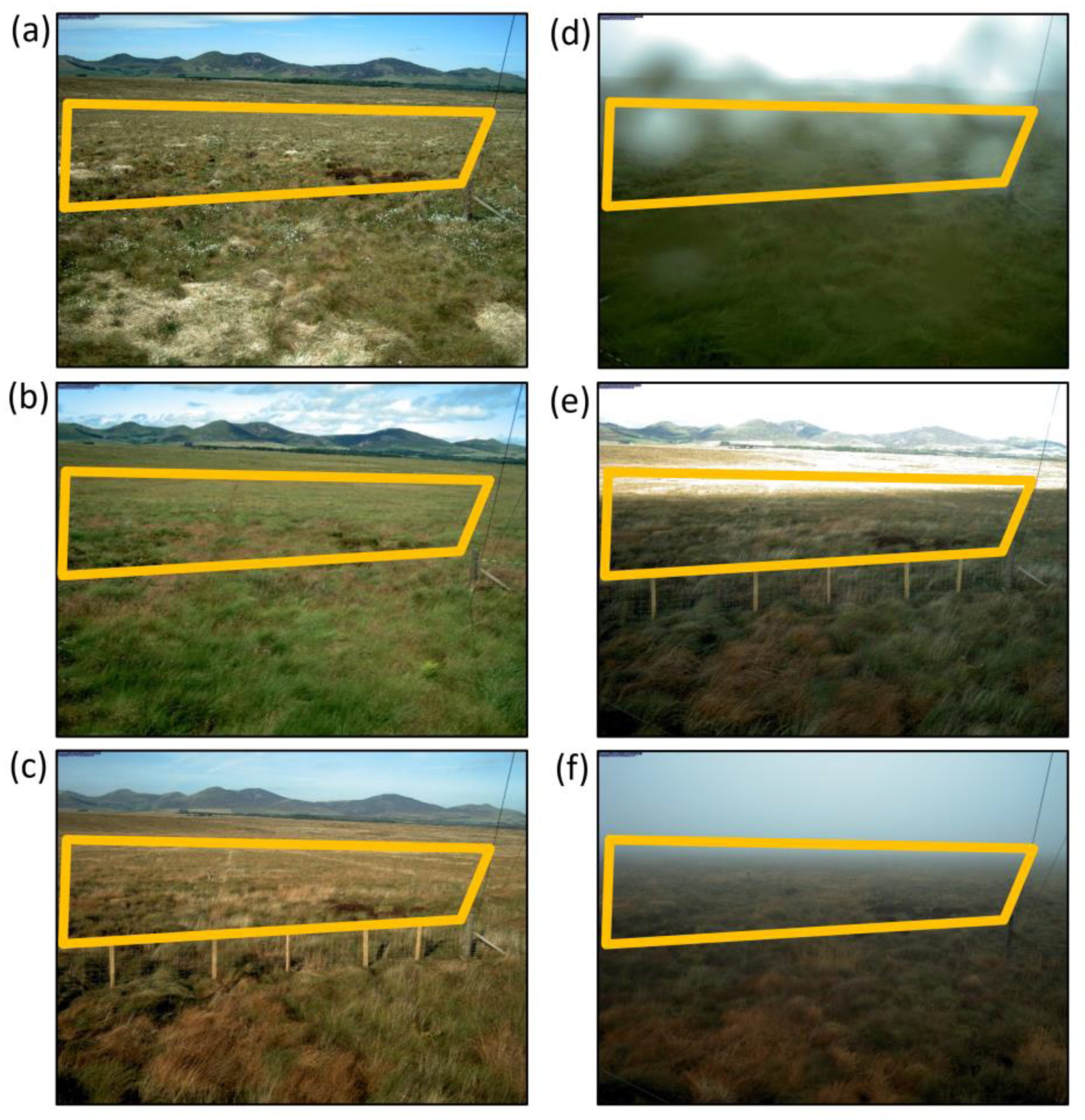
2.3. Phenocam Imagery

Data from a Stardot camera (CAM-SEC5IR, Stardot Technologies, Buena Park, CA, USA) were employed as a near-continuous time-series of green-leaf phenology from its installation in July 2018 until the end of 2021. This phenocam was mounted next to the flux measurement tower (see Figure 1a) at a 3.29 m height, pointing northward (343° N) and inclined downward at a 10° angle. Camera settings adhere to the ICOS phenocam protocol [71], with automatic exposure and a fixed white balance, which is known to improve consistency in the brightness of images taken under variable illumination conditions [72]. Captured RGB images were 5 megapixels in size (2592 × 1944 pixels) and stored as 24-bit JPEG files. We restricted our analysis to imagery collected at midday (12:00 UTC), as this coincided with the average time of the UAV image acquisition. Technical problems with the phenocam setup resulted in some periods of missing data, the largest being in July 2019 (15 days: 10 June–25 June 2019) and August–September 2019 (29 days: 13 August–11 September 2019).

The phenocam imagery was screened for quality. Hereby, images were visually assessed to identify: (i) water condensation on the camera housing; (ii) grazing sheep in the ROI; (iii) snow-cover; or (iv) images with poor illumination conditions (foggy, cloud shadows, sun glint; see Figure 2). All images captured by the above screening were removed from subsequent analysis. RGB images were then processed using the open-source R package, Phenopix [73].

We selected a single region of interest (ROI) outside of the flux measurement compound (see Figure 2) for which colour information in each band was extracted. In each image, the Green Chromatic Coordinate (G_cc) was calculated as the average ‘greenness’ normalised to the total brightness across all bands:

$$G_{cc}={\displaystyle \frac{G_{DN}}{(R_{DN}+G_{DN}+B_{DN})}}$$

(1)

where R, G, and B refer to the red, green and blue bands, respectively, and DN denotes the average digital number (i.e., brightness) of pixels inside the ROI for each band. The G_cc was used as a proxy of phenological development and physiological status of the vegetation canopy. For gaps in the phenocam dataset ≤ 5 days, the data were smoothed using the 90th percentile of G_cc values over three-day moving windows to reduce the impact of variable illumination conditions on the time-series [74]. For the present analysis, gaps > 5 days were not filled, as doing so led to misleading trends at phenological breakpoints, particularly for the large gaps present in the 2019 time-series.

A double logistic model was fitted to the smoothed G_cc time-series to estimate phenological development of the vegetation canopy. Goodness of fit from a selection of models was examined based on their Root Mean Square Error (RMSE; see [73]), and the double logistic model of Gu et al. [75] was employed as this had the lowest RMSE. Finally, changes in slope of the G_cc time-series were used to estimate transition dates of green-leaf phenology, e.g., green-up, peak season, and green-down. This study adopts the phenophase method of Gu et al. [75], in which transition dates for green-up, peak growing season, and green-down are determined by using local extremes of the first-order derivative.

2.4. CO₂ Flux Measurements and Supporting Meteorological Data

2.4.1. Instrumentation

Fluxes of CO₂ were measured continuously using the eddy-covariance (EC) technique and reported for 30-min averaging intervals [76,77,78]. The EC system at Auchencorth Moss has been in operation since 2002 [79], and currently consists of: (i) a closed-path infrared gas analyser (LI-COR 7000, LI-COR Environmental, Inc., Lincoln, NE, USA) measuring water vapour and CO₂ concentrations at 10 Hz (effective height 3.5 m, 20-m long inlet tube, outside diameter 1/4″); and (ii) a 3D ultrasonic anemometer (WindMaster Pro installed at a 3.6-m height was used until June 2019, and then replaced by a HS-50 installed at a 4.1-m height (both Gill Instruments, Lymington, UK)) operating at 20 Hz. Both setups have the same separation (30 cm vertical; 20 cm horizontal) from the inlet of the sampling line and all data were logged to a PC using an in-house LabView^TM program (National Instruments, Austin, TX, USA). In addition to EC measurements, the site is supported by an adjacent meteorological station (see Figure 1; ref. [80]), providing a comprehensive suite of meteorological observations. These measurements include temperature (fine wire type-E thermocouple), water-table depth (WTD, Druck PDCR 1830, Druck Ltd, Leicester, UK), photosynthetically active radiation (PAR, SKP215, Skye Instruments Ltd., Llandrindod, UK) and rainfall (tipping bucket rain gauge). Reference in the text to average meteorological conditions describes long-term values for the period 2002–2017 for all variables except WTD, for which recording began in 2007. Finally, multiple dry spells were observed over the study period, defined here as periods longer than 7 days with WTD > 5 cm below the surface.

2.4.2. Flux Calculation and Quality Screening

Standard EC quality control (Vickers and Mahrt [81]) was applied to CO₂ and H₂O concentrations and wind/turbulence data, as summarised in

Table 4. Outline of EC quality control criteria used in this study.

(1) Data completeness

Check the number of raw data points (N) per 30-min flux averaging period ≥90% of the possible total (i.e., N ≥ 1620 for 10 Hz data)

(2) Raw data spikes

Data excluded if spikes (i.e., values > ± 2 standard deviations from the mean) in vertical wind velocity, CO2 mole fraction, or water-vapour (H2O) mole fraction > 1% total number of data points per 30-min flux averaging period (i.e., ≥18 for 10 Hz data)

(3) Sufficient turbulence

Discard measurements with insufficient turbulence, defined by a friction velocity (u*) threshold [83]

(4) Stationarity

Check that the time-series is in steady state [84]

(5) Flux within sensible range for site

Discard half-hourly CO2 fluxes which fall outside the range ± 30 µ mol CO2 m−2 s−1

. Fluxes were then calculated using the EddyPro software (v7.0.6, LI-COR Biosciences, Inc., Lincoln, NE, USA) and screened to check they were within realistic range for the site. Finally, processed fluxes were quality flagged as part of a 3-point scale [82], where ‘0’ indicates the best-quality fluxes, and ‘2’ indicates the lowest-quality estimates. The latter were discarded from all further analyses.

2.4.3. Flux Partitioning and Gapfilling

The online tool (available at https://bgc.iwww.mpg.de/5622399/REddyProc, accessed on 21 May 2022) developed at the Max Plank Institute for Biogeochemistry (Jena, Germany [85,86]) was used to partition half-hourly NEE fluxes and to fill data gaps resulting from: (i) equipment failure; and (ii) data that did not fulfil the quality requirements in Table 4. Gapfilled data were used to calculate the annual cumulative NEE budgets (as the sum of all half-hourly periods) only, and their associated uncertainty was calculated as the root sum of squares of random uncertainty estimated from the gapfilling analysis for each half-hour period [87].

For the flux partitioning, daytime and missing night-time Reco were modelled based on the temperature response of night-time CO₂ flux data, because these do not contain a photosynthetic uptake component [85,88]. Half-hourly GPP was then calculated as the difference between NEE and Reco. The 90th percentile of daily GPP (GPP90) was used as an indicator of the maximum daily photosynthetic uptake of CO₂ rather than daily averages or totals for example, to reduce the impact of gaps in the dataset. For example, half-hourly periods of missing data (particularly if occurring during daytime) could otherwise bias daily averages of GPP (especially if they are not randomly distributed), or result in lower daily sums of GPP as an artefact of these data gaps

2.5. Statistical Analysis

Statistical analysis was used to examine the strength of the relationship between phenology and GPP over different phenological stages and measurement years. As the data were generally not normally distributed, a Spearman’s rank order correlation (r_s) was employed for all correlation analyses. This exploration of the data involved correlation analysis between single potential predictor variables (G_cc, UAV-derived VIs) and GPP90.

3. Results

3.1. Overview of the Study Period (Hydrometeorological Conditions and CO₂ Balance)

The four years examined were characterized by a number of weather events, which affected both vegetation phenology and physiology, as well as ecosystem functioning. The year 2018 was the most unusual year with respect to the long-term record. Cold conditions and late snowfall during spring led to a delayed start to the growing season, and were followed by a European-wide summer heat and drought event [89,90]. Monthly air temperatures in June and July were consistently above the long-term average, and the site experienced a dry spell (defined as a period longer than 7 days with WTD more than 5 cm below the surface) of over two months. During this period WTD remained below 10 cm for 77 days (28 June to 12 September 2018), and reached a minimum of 47 cm (Figure 3). From visual field observation, this dry spell resulted in the desiccation of vegetation and early senescence. This year was also unique in terms of its CO₂ budget. Coinciding with the warm, dry conditions, the year 2018 had a positive NEE (7.92 ± 0.5 mol CO₂ m⁻² y⁻¹), which is in contrast to the long-term sink function observed at the site [79,91]. Unusually, daily cumulative NEE did not cross the zero line at any point during this year, and instead remained consistently positive.

The year 2019 was characterised by more normal conditions with respect to the long-term (2002–2017) average. This year experienced a warm start, with monthly Tair in February 2019 being almost twice the average, and daily mean Tair was consistently above zero from early February (day of year (DOY) 35). It follows that the growing season also commenced early during this year, with green-up in late April (see

Table 5. Phenological stages for the study years estimated using the phenocam data. Shown are the estimated start and end DOY for green-up, peak growing season, green-down, and the complete growing season (i.e., start of green-up to end of green-down). The overall length of each period is shown in brackets. Note: no estimation of phenological breakpoints was conducted for the year 2018, because the time series of images available after camera installation (July 2018) was too short to estimate greenness trajectory over the growing season.

Year	Green-Up	Peak Growing Season	Green-Down	Complete Growing Season
2018	-	-	-	-
2019	DOY 119–156 (37 days)	DOY 156–269 (113 days)	DOY 269–321 (52 days)	DOY 119–321 (202 days)
2020	DOY 127–186 (59 days)	DOY 186–253 (67 days)	DOY 253–317 (64 days)	DOY 127–317 (190 days)
2021	DOY 135–171 (36 days)	DOY 171–254 (83 days)	DOY 254–329 (75 days)	DOY 135–329 (194 days)

). All months were wetter than average from April onwards, although there were a few dry spells, the most notable of which occurred on DOY 105–128 (23 days, mid-April to early May; Figure 3). Summer WTD was closer to the surface than in 2018, with mean WTD in July for example being close to average (WTD anomaly for July 2019 = + 3.7 cm, vs. + 30.7 cm for July 2018; both with respect to the 2007–2017 average), and Tair for the rest of the year was within average range for the site. Zero-crossing of cumulative NEE (i.e., when cumulative NEE first became negative), occurred on DOY 166, and over this year the peatland functioned as a net sink of atmospheric CO₂ (annual budget = −2.73 ± 0.6 mol CO₂ m⁻² y⁻¹).

The year 2020 had a dry start to the growing season and was affected by the longest dry spell in the study period (84 days: 7 April–29 June 2020; Figure 3). This year also exhibited the shortest growing season, characterised by a prolonged green-up period (>20 days longer than estimated for the other years) and a short peak (ca. 60% shorter than for other years; see Table 5). The ecosystem functioned as a net source of CO₂ to the atmosphere (annual NEE = 4.04 ± 0.5 mol CO₂ m⁻² y⁻¹) and there was a delay in the zero-crossing date of cumulative NEE, which did not occur until the end of July (for 2019 and 2021, this occurred in mid-June).

Finally, the year 2021 experienced a cooler than average spring (1.4 °C below the long-term average, March–May), and was affected by multiple dry spells during summer and autumn (Figure 3). In terms of phenological development, 2021 was notably different to the rest of the study period. This year displayed an asymmetrical greenness curve, characterized by a delayed, but rapid greening; and a more gradual, prolonged senescence period (Figure 4, Table 5). Greenness values peaked shortly after the transition to the peak growing season, before declining towards the end of the growing season in tandem with frequent dry spells. The annual CO₂ budget for this year was close to, and not statistically different from, zero (NEE = 0.03 ± 0.6 mol CO₂ m⁻² y⁻¹).

3.2. Monitoring Vegetation Phenology

The two phenology datasets (phenocam, UAV) differed considerably in their spatial, temporal, and spectral resolution, and are described in detail below. Note that the term ‘greenness’ is used to describe both the UAV-derived VIs (Table 3) and phenocam-derived G_cc (Equation (1)).

3.2.1. Phenocam Data

The phenocam data provide a near-continuous time-series of vegetation phenology from mid-2018 until the end of 2021. Although the G_cc is a simple index and not spectrally calibrated, it was able to capture a clear seasonal trend in greenness at the site (see Figure 4). Four phenological phases were identified: (1) green-up, characterised by a steep rise in greenness during spring as the vegetation canopy begins to develop; (2) a peak growing season, where greenness values plateau during the summer once the vegetation canopy is fully developed; (3) green-down, characterised by a rapid reduction in greenness as the canopy starts to senesce; and (4) a dormant phase, represented by relatively stable, low greenness values either side of the growing season. Day-to-day variability was observed in the time-series, particularly when seasonal changes in greenness were low (e.g., during the shoulder seasons). Here, noise in the dataset was observed to exceed temporal trends in greenness.

3.2.2. UAV Data

The spectrally calibrated UAV data, despite their coarser temporal resolution (bi-weekly to monthly), were able to capture trends in vegetation phenology. Time-series of UAV-derived VIs averaged over the study area were generally consistent with the phenocam data (Figure 4), and a strong correlation was identified between phenocam- and UAV-derived greenness for all calculated VIs (see Figure 5, r_s = 0.77–0.86, p < 0.01). However, peak greenness values in 2019 and 2021 were notably different. Here the UAV-derived VIs indicated a similar greenness over the two years, whereas phenocam-derived G_cc indicated a greater peak greenness during the 2021 growing season (maximum G_cc = 0.44, Figure 4).

3.2.3. Capturing Spatial and Temporal Variability Within the Growing Season

Phenocam-derived G_cc was calculated as an average for the entire ROI, hence smoothing out the spatial variability observed in the imagery (Figure 2). In contrast, the spatially referenced UAV-derived VIs revealed a strong heterogeneity in greening across the survey area. This heterogeneity can be seen in Figure 6, which maps the pixel-wise change in greenness between surveys conducted in the early (14 May 2021) and peak growing season (3 August 2021). Although, greening was observed across the scene, the area to the northeast exhibited a more pronounced greening than the rest of the survey area. These pixels correspond to areas with a dominant vegetation cover of the deciduous grass species, M. caerulea.

We extracted VIs for each species by overlaying the UAV survey data and species-level classification map (see Figure 1). Overall, we found that the shrubs C. vulgaris and Vaccinium spp. and the grass, M. caerulea, displayed the largest seasonal amplitude (i.e., growing season peak to trough, see Figure 7) in greenness for the calculated VIs. In contrast, mosses (P. schreberi, Sphagnum spp.) and the rush, J. effusus, exhibited the smallest seasonal amplitude and lowest peak greenness values of all species examined. Towards the start and end of the growing season, we observed that variability in the VIs at the species-level was relatively small (Figure 7). However, heterogeneity in greenness across the individual species increased substantially over the summer months once the canopy had developed.

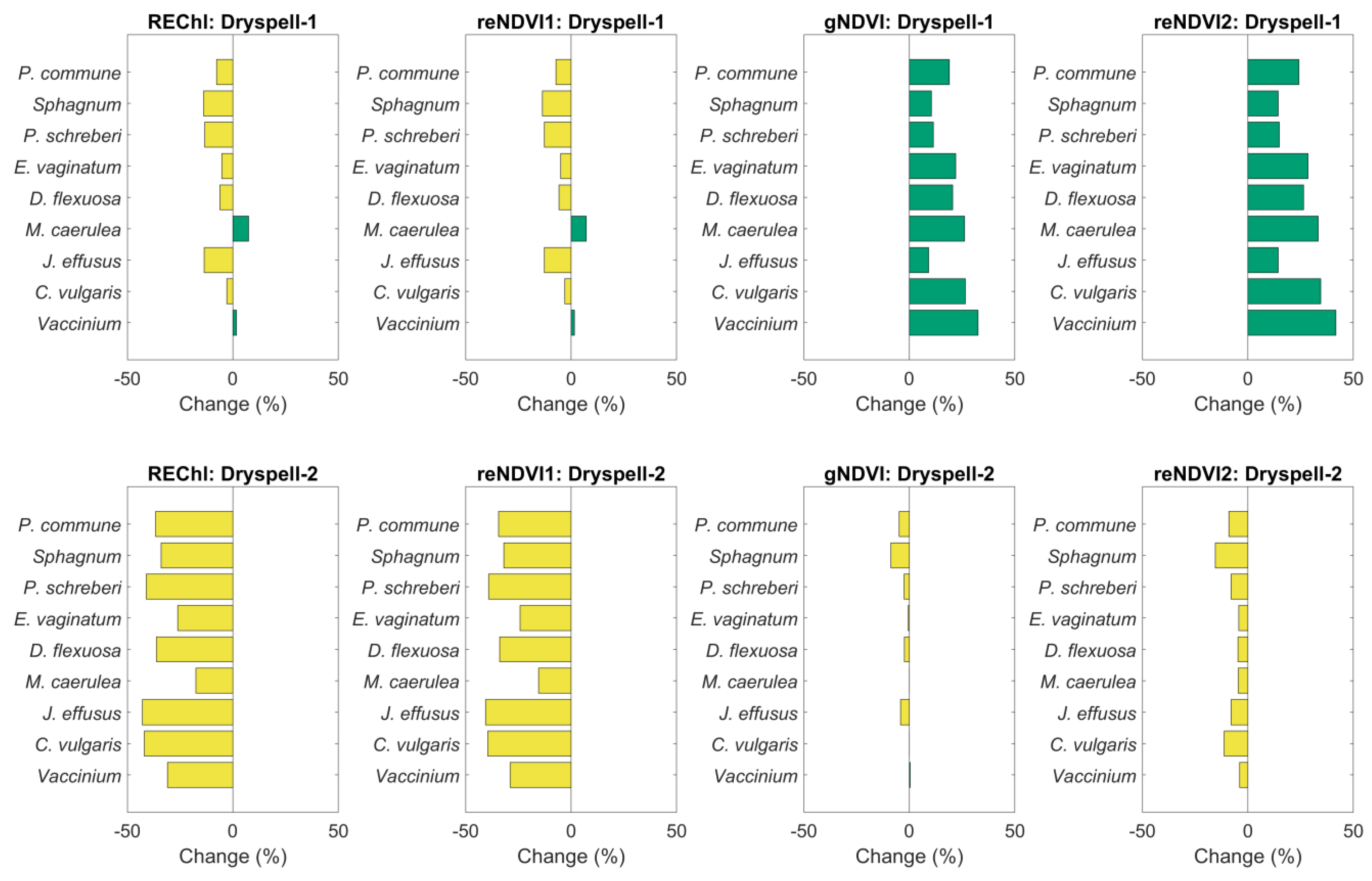
3.2.4. Sensitivity of the Phenological Datasets to Drought

Changes in greenness captured by UAV surveys in 2021 were examined over two dry spells. The first of these dry spells, ‘Dryspell-1’, occurred during green-up, extending from DOY 158–193; and the second, ‘Dryspell-2’, occurred during the peak growing season from DOY 200–223 (see Figure 7). We identified differences in: (i) the sensitivity of the various UAV-derived VIs; and (ii) the species-level response to the dry conditions.

As shown in Figure 8, for Dryspell-1 no reduction in greenness for any species was apparent when examining the VIs gNDVI and reNDVI2 (Figure 8, upper row). In contrast, we observed a substantial reduction in greenness for the VIs REChl and reNDVI1. For these indices, the maximum observed reduction in greenness for individual species was ca. 13% of their seasonal cycle, except for M. caerulea which displayed a slight greening throughout the dry spell. In contrast, during Dryspell-2 all indices displayed more sensitivity to drought, with a reduction in greenness observed in all cases except for M. caerulea and Vaccinium spp. when using the gNDVI (Figure 8, bottom row). For the indices REChl and reNDVI1, reductions in the greenness of pixels containing J. effusus, P. schreberi, and C. vulgaris were substantial (ca. 40% of their seasonal amplitude). In contrast, gNDVI and reNDVI2 were less sensitive, with maximum reductions in greenness observed for pixels dominated by Sphagnum spp. (ca. 9% and 15% of seasonal amplitude for the gNDVI and reNDVI2, respectively).

3.3. Seasonal and Inter-Annual Variability in the Relationship Between GPP and Phenology

Both the phenocam- and UAV-derived VIs were found to exhibit a strong correlation with GPP90. Correlation coefficients were >0.70 (r_s, p < 0.01) for all indices except the NGRDI, for which correlation was moderate (r_s = 0.57, p < 0.05). Variability in the strength of the relationship between species-level VIs and GPP90 was low. Using the index reNDVI1 as an example, correlation between GPP90 and reNDVI1 for the survey area was 0.78 (r_s, p < 0.01) and species values ranged from r_s = 0.72 (Sphagnum spp.) to r_s = 0.78 (C. vulgaris; p < 0.01 for all).

The phenocam dataset, with its high temporal coverage, facilitated examination of the above relationships in more detail. For the complete time-series (all years combined), changes in canopy greenness were observed to follow the same seasonal cycle as daily GPP90, and these two variables displayed a strong correlation (r_s = 0.88, p < 0.01). This bulk analysis, however, masks a large amount of seasonal variability, as illustrated in Figure 9. For example, during the peak growing season when the canopy was fully developed, the relationship between daily GPP90 and G_cc was not statistically significant for any year. The strongest relationships between greenness and GPP90 were observed during green-down and green-up (Figure 9). One discrepancy was the weak correlation between GPP90 and G_cc observed in the 2019 green-up (r_s = 0.39, p < 0.05). These results indicate an inter-annual and seasonal variability in the relationship between observed vegetation greenness and GPP at Auchencorth Moss.

4. Discussion

4.1. Monitoring Vegetation Phenology

Monitoring vegetation remotely (e.g., satellite, phenocam, UAV) is key to understanding phenological controls on carbon fluxes. The two phenological datasets employed in this study contrasted in their spatial, temporal, and spectral resolutions. The main strengths and weaknesses of each are outlined below, alongside a discussion of some key problems to consider when comparing across phenology datasets.

4.1.1. Phenocam Data

The phenocam imagery at Auchencorth Moss had a number of limitations for monitoring phenology. Firstly, the combined effect of camera inclination, the patchy nature of vegetation, and the strong micro-topography at the site made it difficult to examine greenness trajectories of the individual species. Although not conducted with imagery from our instrument setup, pixel-level analysis of phenocam imagery is possible and has been performed across a range of ecosystems to highlight spatial variability in vegetation phenology [42,53,73]. Secondly, the phenocam imagery used in the present study was not spectrally calibrated as the UAV data were. Brightness values for each band were variable across images and influenced by weather conditions during image capture. In our study, we conducted a visual inspection to screen poor-quality images from analysis (i.e., those affected by sun-glint, lens flare, variable scene illumination conditions, see Figure 2). This level of quality control is however rare in phenocam studies, where quality filtering is not standardised and a range of approaches are used [72,92,93]. Despite the adoption of the recommended ‘fixed white balance’ camera setting and the 90th percentile of 3-day G_cc values [74], the lack of spectral calibration and limited quality control of phenocam data mean that the calculated index (i.e., G_cc) has poor accuracy and cannot be reliably compared across sites or between discrete points in time. This limits analysis to broad phenological trends over periods of weeks, rather than direct comparison between days, where differences in illumination and meteorology during image capture likely exceed changes in greenness. Here. it is important that protocols (e.g., the use of reference panels; [72,93]) are developed surrounding the calibration of phenocam imagery and that a standardised, robust approach for quality filtering the collected imagery is developed.

Despite these caveats, phenocams are valuable tools for monitoring peatland phenology. In this study, phenocam-derived G_cc: (i) captured the seasonal trend in greenness at the site; and (ii) displayed a strong correlation with spectrally calibrated UAV data. The near-continuous temporal coverage and automated monitoring facilitated by phenocams allow for large amounts of data collection, which are particularly valuable for estimating the timing of phenological stages and monitoring change [34,35]. Furthermore, phenocams are often installed alongside EC setups [43], and as such, can provide important datasets to study the impact of phenology on inter-annual variability in CO₂ flux (e.g., ref. [94]). Improving the understanding of changes in phenology on peatland carbon balance will be key to predicting the long-term response of these ecosystems to climate change.

4.1.2. UAV Data

A high temporal resolution can be challenging to achieve with UAV surveys due to weather constraints. However, UAV data, when calibrated correctly and following a robust workflow, do provide spatially geo-referenced data of high spectral resolution and quality. The multispectral Parrot Sequoia camera setup employed in the present study acquired data in both the Red-Edge and NIR bands, which are more sensitive to physiological changes than bands in the visible spectrum. Analysis found that UAV-derived VIs centred on these bands (e.g., reNDVI1) were more sensitive to the impacts of abiotic change on the canopy. During dry spells, we observed reductions in UAV-derived VIs equating to around 40% of the seasonal amplitude in greenness, which were not visible in the phenocam data. Incorporating data from the short-wave infrared (SWIR) region may improve our ability to study the impact of drought events on vegetation, and such VIs have been successfully used to detect moisture stress in peatland environments, both as a whole and in particular species such as Sphagnum [95,96]. The use of additional VIs may improve the correlation between phenology and flux datasets, although this could not be tested with our presented setup. Finally, the future use of UAVs in peatland phenology research at a range of sites could improve understanding of the impact of short- (e.g., response to weather events) and long-term environmental change (e.g., response to climate change) on peatland vegetation.

4.1.3. Problems Comparing Phenological Datasets

Studies utilising phenological data from multiple sensors (e.g., comparing phenocam with UAV or satellite data) face a number of challenges. Firstly, the accurate comparison of datasets relies on the assumption that all sensors are observing the same vegetation phenology [56,97,98]. The two camera systems employed in the present study (phenocam, multispectral) had different and non-overlapping fields of view. The phenocam was mounted next to the EC tower (Figure 1a) and viewed vegetation to the north (oriented in line with phenocam protocol; [71]). In contrast, the multispectral sensor on the UAV acquired data over the predominant flux footprint area south-west of the EC tower. Despite these differences, based on expert knowledge of vegetation at the site, including extensive quadrat surveys for ICOS and other long-term monitoring activities [99], vegetation composition captured by the phenocam was assumed to be representative of the UAV survey area. Although treated with caution, the similar temporal trends in greenness of the two datasets suggest that vegetation communities monitored by both setups were comparable (see Figure 4).

Secondly, as vegetation canopies are non-Lambertian surfaces, viewing geometry has a strong impact on the signal measured by the sensor and any calculated VIs [100,101,102]. In the present study, the phenocam had an oblique viewing angle, whereas the UAV imagery was collected at nadir. The size of this impact on calculated VIs can be large. A study by Epiphanio and Huete [101], for example, found that NDVI calculated from measurements conducted with a viewing angle (as opposed to nadir) differed from their counterparts by as much as 50%. Studies comparing phenocam and remote sensing data also find that differences in viewing geometry lead to disparity in calculated phenological transition dates [98,103]. Phenocams, for example, may observe a more rapid senescence of vegetation than satellite data, as their oblique viewing angle enables them to better capture senescing flowers and grass stems compared to the nadir view of aerial imagery [104]. Although the present study did not compare phenological transition dates from the two datasets, this is an important aspect to consider in future work.

Finally, monitoring vegetation phenology from above (i.e., from nadir with the UAV, or from a viewing angle as with the phenocam) in ecosystems with complex multi storey canopies (e.g., peatlands, grasslands) can be problematic, for example because of shading, and the fact that a number of species (e.g., Nardus stricta, M. caerulea) green structurally from the bottom up. These structural differences can create a time lag between flux- and remotely sensed phenology datasets, as the latter will only register greening of the upper canopy. In an alpine grassland ecosystem, Migliavacca et al. [105] estimated the size of this lag to be around one week. Although in the present study, we observed strong correlations between GPP and phenocam-derived G_cc, viewing geometry has an important influence on the relationship between VIs and CO₂ fluxes, particularly during the green-up stage.

4.2. Links Between Vegetation Greenness and Ecosystem Functioning

Using four years of phenocam imagery and UAV data at the site, peatland vegetation phenology was found to be a strong predictor of GPP. Both phenocam-derived G_cc and UAV-derived VIs (particularly those employing the red-edge band, e.g., the reNDVI1) displayed strong correlations with GPP estimates, despite notable differences in the quality of the two phenological datasets. This strong relationship between GPP and phenocam-derived greenness is in agreement with observations from a number of studies [53,94,106,107,108].

In the present study, phenocam-derived greenness displayed the strongest correlation with GPP during green-up and green-down. In contrast, during the peak growing season when the vegetation canopy was fully developed, the relationship between G_cc and GPP was not statistically significant (p > 0.05). This finding indicates that meteorological conditions, rather than vegetation greenness likely control GPP during the peak growing season. Such strong seasonal variability in the drivers of CO₂ flux has been observed at a number of peatland sites [53,94,109]. Although phenology acts as a dominant control over peatland carbon dynamics during the transition seasons (i.e., when the vegetation canopy is developing), abiotic conditions such as temperature and WTD play a key role in regulating CO₂ exchange during the peak growing season [53,94,109]. Interactions between peatland phenology, weather and GPP are, however, complex. In a regional study of European peatlands, for example, Koebsch et al. [94] identified phenology as a key predictor of variability in photosynthetic CO₂ uptake at the seasonal level, and showed that temperature and radiation affected GPP indirectly, by influencing plant phenology. Such regional studies provide valuable insights that can be used to better characterise the role of vegetation phenology in terrestrial ecosystem models (e.g., ref. [110]).

4.3. Impact of Dry Spells

The present study highlighted the strong impact of weather anomalies on peatland vegetation and ecosystem functioning. We observed that years with prolonged or frequent dry spells functioned as a net source of CO₂ to the atmosphere, which is in contrast with the long-term net uptake measured at the site [79,91]. Numerous studies have linked drought conditions to a short-term reduction in peatland C uptake [17,33,79]. The associated lowering of WTD, which is a key control on GPP [91,111], can induce vegetation stress and limit CO₂ uptake by canopy photosynthesis (e.g., due to stomatal closure). In particular, our results have highlighted the importance of the timing and duration of dry spells. When dry conditions occurred during green-up (as in the year 2020), we observed a slower development of the vegetation canopy, which causes a substantial delay in cumulative NEE zero-crossing date. Consequently, the peak growing season begins later and is shorter than normal, meaning we observe a reduced period of optimum canopy development and maximum rates of photosynthesis. Changes in the timing and duration of plant canopy development likely made a substantial contribution to the positive annual NEE budget recorded during our study in the year 2020 (i.e., net loss of CO₂). In contrast, the favourable hydrometeorological conditions during green-up 2021 allowed the canopy to green strongly and rapidly, meaning that the vegetation canopy was fully developed earlier, with a high photosynthetic capacity. Here, we hypothesise that the frequent dry spells experienced during the summer and autumn of this year induced early senescence. The importance of timing on the impact of drought events has been reported previously by Lund et al. [17] for a temperate Swedish peatland. The authors found that a short, severe drought during the peak growing season, when the vegetation canopy was fully developed, had no significant impact on GPP. However, a longer drought period during spring green-up (when the canopy was developing), resulted in a reduction in GPP rates. Studies suggest that during this stage of canopy development, GPP shows the strongest sensitivity and is the least resilient to drought [17,32]. Similar results have been found in response to heatwaves, with delayed greening observed in an alpine grassland and a 40% reduction in phenocam canopy greenness [42]; which is of similar magnitude to what the present study observed with the UAV data for Dryspell-2.

Finally, the community-level response to drought in peatland ecosystems is influenced by species composition (e.g., refs. [112,113]). Vascular plants, with their developed root systems, are generally more tolerant to the effects of periodic drought than Sphagnum spp., for example, which have no root systems (e.g., ref. [114]). In the present study, we employed the spatially referenced UAV data to highlight the differing response of the mapped species to dry conditions (Figure 7 and Figure 8). We found that M. caerulea and E. vaginatum with their deep root systems [115,116] appeared less sensitive (i.e., exhibited a smaller or no reduction in greenness) to the dry conditions compared to species with shallow (e.g., J. effusus [117]) or no roots (e.g., Sphagnum spp., P. commune). Although not possible with our employed setup, pixel-level analysis can also be conducted on phenocam imagery, and used to examine variability across plant functional types (e.g., Ref. [42]). These two monitoring approaches hence allow fine-scale heterogeneity in species response to drought to be quantified, and can be used to detect changes in ecosystem functioning not possible with the coarser resolution of satellite data. Such research is key for monitoring the response of peatland ecosystems to future change.

5. Conclusions

Vegetation phenology plays a strong role in the inter-annual variability of the peatland carbon balance [108,109,118], and will be affected by both long-term climate change and an associated increase in the frequency of extreme weather events [30]. As such, phenological monitoring is key to improving predictions of the future fate of peatland carbon stocks under climate change. However, the remoteness of many peatland ecosystems means that traditional phenological datasets are limited. Furthermore, due to the pronounced spatial heterogeneity of peatlands, satellite data products are unable to accurately capture variability in their phenology [62].

The present study examined the use of phenocam imagery and the novel approach of multi-temporal UAV surveying to monitor the phenology of peatland vegetation over a number of growing seasons. Both methods were suitable for characterising peatland phenology, although they differed in terms of their relative merits and weaknesses. The high temporal resolution of phenocam data (daily) was invaluable for identifying the different stages of phenological development. Such high temporal coverage was not feasible with manual UAV surveys, although these provided us with discrete time points of rich data to supplement the limited spatial and spectral resolution provided by phenocam imagery. We found that collection of spectral data in the red-edge and NIR bands was advantageous, in that VIs employing these bands were more sensitive to dry spells. Furthermore, we demonstrated the potential of UAV surveys for monitoring spatial heterogeneity in the phenology of peatland vegetation, which can be difficult to achieve with phenocam data (e.g., depending on site characteristics, camera viewing angle). Both datasets displayed a strong correlation with peatland GPP. For the UAV data, we found that VIs utilising the red-edge band (e.g., the reNDVI1) were best able to predict GPP at the site, partly because these indices were most sensitive to physiological changes such as drought. However, analysis of the high temporal resolution phenocam dataset was able to highlight a large amount of inter-annual and seasonal variability in the strength of this relationship.

The years examined in the present study were unusual with respect to the long-term measurement record at the site, with frequent dry spells and a tendency for the peatland to function as a net source of CO₂. Our findings suggest that the seasonal timing of future weather anomalies will be a key factor determining their impact on the peatland carbon balance. Continued long-term monitoring of peatland ecosystems and their vegetation is crucial to improving our understanding of the current drivers of peatland CO₂ dynamics and how these may change in the future.

References

1. Keenan, T.F.; Williams, C.A. The Terrestrial Carbon Sink. Annu. Rev. Environ. Resour. 2018, 43, 219–243. [Google Scholar] [CrossRef]
2. D’Arrigo, R.; Jacoby, G.C.; Fung, I.Z. Boreal Forests and Atmosphere–Biosphere Exchange of Carbon Dioxide. Nature 1987, 329, 321–323. [Google Scholar] [CrossRef]
3. Hall, C.A.S.; Ekdahl, C.A.; Wartenberg, D.E. A Fifteen-Year Record of Biotic Metabolism in the Northern Hemisphere. Nature 1975, 255, 136–138. [Google Scholar] [CrossRef]
4. Lieth, H. Phenology in Productivity Studies. In Analysis of Temperate Forest Ecosystems; Reichle, D.E., Ed.; Springer: Berlin/Heidelberg, Germany; New York, NY, USA, 1970; pp. 29–46. [Google Scholar]
5. Richardson, A.D.; Keenan, T.F.; Migliavacca, M.; Ryu, Y.; Sonnentag, O.; Toomey, M. Climate Change, Phenology, and Phenological Control of Vegetation Feedbacks to the Climate System. Agric. For. Meteorol. 2013, 169, 156–173. [Google Scholar] [CrossRef]
6. Buitenwerf, R.; Rose, L.; Higgins, S.I. Three Decades of Multi-Dimensional Change in Global Leaf Phenology. Nat. Clim. Chang. 2015, 5, 364–368. [Google Scholar] [CrossRef]
7. Cleland, E.E.; Chuine, I.; Menzel, A.; Mooney, H.A.; Schwartz, M.D. Shifting Plant Phenology in Response to Global Change. Trends Ecol. Evol. 2007, 22, 357–365. [Google Scholar] [CrossRef]
8. Menzel, A.; Yuan, Y.; Matiu, M.; Sparks, T.; Scheifinger, H.; Gehrig, R.; Estrella, N. Climate Change Fingerprints in Recent European Plant Phenology. Glob. Change Biol. 2020, 26, 2599–2612. [Google Scholar] [CrossRef]
9. Parmesan, C.; Yohe, G. A Globally Coherent Fingerprint of Climate Change Impacts across Natural Systems. Nature 2003, 421, 37–42. [Google Scholar] [CrossRef]
10. Walther, G.R.; Post, E.; Convey, P.; Menzel, A.; Parmesan, C.; Beebee, T.J.C.; Fromentin, J.M.; Hoegh-Guldberg, O.; Bairlein, F. Ecological Responses to Recent Climate Change. Nature 2002, 416, 389–395. [Google Scholar] [CrossRef]
11. Badeck, F.W.; Bondeau, A.; Böttcher, K.; Doktor, D.; Lucht, W.; Schaber, J.; Sitch, S. Responses of Spring Phenology to Climate Change. New Phytol. 2004, 162, 295–309. [Google Scholar] [CrossRef]
12. Jeong, S. Autumn Greening in a Warming Climate. Nat. Clim. Chang. 2020, 10, 712–713. [Google Scholar] [CrossRef]
13. Jeong, S.J.; Ho, C.H.; Gim, H.J.; Brown, M.E. Phenology Shifts at Start vs. End of Growing Season in Temperate Vegetation over the Northern Hemisphere for the Period 1982–2008. Glob. Change Biol. 2011, 17, 2385–2399. [Google Scholar] [CrossRef]
14. Peñuelas, J.; Rutishauser, T.; Filella, I. Phenology Feedbacks on Climate Change. Science 2009, 324, 887–888. [Google Scholar] [CrossRef] [PubMed]
15. Seneviratne, S.I.; Zhang, X.; Adnan, M.; Badi, W.; Dereczynski, C.; Di Luca, A.; Ghosh, S.; Iskandar, I.; Kossin, J.; Lewis, S.; et al. Weather and Climate Extreme Events in a Changing Climate. In Climate Change 2021: The Physical Science Basis. Contribution of Working Group I to the Sixth Assessment Report of the Intergovernmental Panel on Climate Change; Masson-Delmotte, V., Zhai, P., Pirani, A., Connors, S.L., Péan, C., Berger, S., Caud, N., Chen, Y., Goldfarb, L., Gomis, M.I., Huang, M., et al., Eds.; Cambridge University Press: Cambridge, UK; New York, NY, USA, 2021; pp. 1513–1766. [Google Scholar]
16. Alm, J.; Schulman, L.; Walden, J.; Nykänen, H.; Martikainen, P.J.; Silvola, J. Carbon Balance of a Boreal Bog during a Year with an Exceptionally Dry Summer. Ecology 1999, 80, 161–174. [Google Scholar] [CrossRef]
17. Lund, M.; Christensen, T.R.; Lindroth, A.; Schubert, P. Effects of Drought Conditions on the Carbon Dioxide Dynamics in a Temperate Peatland. Environ. Res. Lett. 2012, 7, 045704. [Google Scholar] [CrossRef]
18. Keeling, C.D.; Chin, J.F.S.; Whorf, T.P. Increased Activity of Northern Vegetation Inferred from Atmospheric CO2 Measurements. Nature 1996, 382, 146–149. [Google Scholar] [CrossRef]
19. Piao, S.; Liu, Q.; Chen, A.; Janssens, I.A.; Fu, Y.; Dai, J.; Liu, L.; Lian, X.; Shen, M.; Zhu, X. Plant Phenology and Global Climate Change: Current Progresses and Challenges. Glob. Change Biol. 2019, 25, 1922–1940. [Google Scholar] [CrossRef]
20. Gorham, E. Northern Peatlands: Role in the Carbon Cycle and Probable Responses to Climatic Warming. Ecol. Appl. 1991, 1, 182–195. [Google Scholar] [CrossRef]
21. Yu, Z.C. Northern Peatland Carbon Stocks and Dynamics: A Review. Biogeosciences 2012, 9, 4071–4085. [Google Scholar] [CrossRef]
22. Limpens, J.; Berendse, F.; Blodau, C.; Canadell, J.G.; Freeman, C.; Holden, J.; Roulet, N.; Rydin, H.; Schaepman-Strub, G. Peatlands and the Carbon Cycle: From Local Processes to Global Implications—A Synthesis. Biogeosciences 2008, 5, 1475–1491. [Google Scholar] [CrossRef]
23. Tarnocai, C.; Stolbovoy, V. Northern Peatlands: Their Characteristics, Development and Sensitivity to Climate Change. Dev. Earth Surf. Process. 2006, 9, 17–51. [Google Scholar] [CrossRef]
24. Callaghan, T.V.; Bergholm, F.; Christensen, T.R.; Jonasson, C.; Kokfelt, U.; Johansson, M. A New Climate Era in the Sub-Arctic: Accelerating Climate Changes and Multiple Impacts. Geophys. Res. Lett. 2010, 37, L14705. [Google Scholar] [CrossRef]
25. Hoegh-Guldberg, O.; Jacob, D.; Taylor, M.; Bindi, M.; Brown, S.; Camilloni, I.; Diedhiou, A.; Djalante, R.; Ebi, K.L.; Engelbrecht, F.; et al. Impacts of 1.5 °C Global Warming on Natural and Human Systems. In Global Warming of 1.5 °C. An IPCC Special Report on the Impacts of Global Warming of 1.5 °C Above Pre-Industrial Levels and Related Global Greenhouse Gas Emission Pathways, in the Context of Strengthening the Global Response to the Threat of Climate Change; IPCC; Masson-Delmotte, V., Zhai, P., Pörtner, H.-O., Roberts, D., Skea, J., Shukla, P.R., Pirani, A., Moufouma-Okia, W., Péan, C., Pidcock, R., et al., Eds.; Cambridge University Press: Cambridge, UK; New York, NY, USA, 2018; pp. 175–312. [Google Scholar] [CrossRef]
26. Dise, N.B. Peatland Response to Global Change. Science 2009, 326, 810–811. [Google Scholar] [CrossRef]
27. Gonsamo, A.; Chen, J.M.; Ooi, Y.W. Peak Season Plant Activity Shift towards Spring Is Reflected by Increasing Carbon Uptake by Extratropical Ecosystems. Glob. Change Biol. 2018, 24, 2117–2128. [Google Scholar] [CrossRef] [PubMed]
28. Gu, L.; Post, W.M.; Baldocchi, D.; Andy Black, T.; Verma, S.B.; Vesala, T.; Wofsy, S.C. Phenology of Vegetation Photosynthesis. In Phenology: An Integrative Environmental Science. Tasks for Vegetation Science; Schwartz, M.D., Ed.; Springer: Dordrecht, The Netherlands, 2003; Volume 39, pp. 467–485. [Google Scholar]
29. Peñuelas, J.; Filella, I. Responses to a Warming World. Science 2001, 294, 793–795. [Google Scholar] [CrossRef]
30. Antala, M.; Juszczak, R.; van der Tol, C.; Rastogi, A. Impact of Climate Change-Induced Alterations in Peatland Vegetation Phenology and Composition on Carbon Balance. Sci. Total Environ. 2022, 827, 154294. [Google Scholar] [CrossRef] [PubMed]
31. Piao, S.; Friedlingstein, P.; Ciais, P.; Viovy, N.; Demarty, J. Growing Season Extension and Its Impact on Terrestrial Carbon Cycle in the Northern Hemisphere over the Past 2 Decades. Glob. Biogeochem. Cycles 2007, 21, GB3018. [Google Scholar] [CrossRef]
32. Barel, J.M.; Moulia, V.; Hamard, S.; Sytiuk, A.; Jassey, V.E.J. Come Rain, Come Shine: Peatland Carbon Dynamics Shift Under Extreme Precipitation. Front. Environ. Sci. 2021, 9, 233. [Google Scholar] [CrossRef]
33. Lafleur, P.M.; Roulet, N.T.; Bubier, J.L.; Frolking, S.; Moore, T.R. Interannual Variability in the Peatland-Atmosphere Carbon Dioxide Exchange at an Ombrotrophic Bog. Glob. Biogeochem. Cycles 2003, 17, 1036. [Google Scholar] [CrossRef]
34. Brown, T.B.; Hultine, K.R.; Steltzer, H.; Denny, E.G.; Denslow, M.W.; Granados, J.; Henderson, S.; Moore, D.; Nagai, S.; Sanclements, M.; et al. Using Phenocams to Monitor Our Changing Earth: Toward a Global Phenocam Network. Front. Ecol. Environ. 2016, 14, 84–93. [Google Scholar] [CrossRef]
35. Richardson, A.D. Tracking Seasonal Rhythms of Plants in Diverse Ecosystems with Digital Camera Imagery. New Phytol. 2019, 222, 1742–1750. [Google Scholar] [CrossRef]
36. Richardson, A.D. PhenoCam: An Evolving, Open-Source Tool to Study the Temporal and Spatial Variability of Ecosystem-Scale Phenology. Agric. For. Meteorol. 2023, 342, 109751. [Google Scholar] [CrossRef]
37. Arndt, K.A.; Santos, M.J.; Ustin, S.; Davidson, S.J.; Stow, D.; Oechel, W.C.; Tran, T.T.P.; Graybill, B.; Zona, D. Arctic Greening Associated with Lengthening Growing Seasons in Northern Alaska. Environ. Res. Lett. 2019, 14, 125018. [Google Scholar] [CrossRef]
38. Arroyo-Mora, J.P.; Kalacska, M.; Soffer, R.; Ifimov, G.; Leblanc, G.; Schaaf, E.S.; Lucanus, O. Evaluation of Phenospectral Dynamics with Sentinel-2A Using a Bottom-up Approach in a Northern Ombrotrophic Peatland. Remote Sens. Environ. 2018, 216, 544–560. [Google Scholar] [CrossRef]
39. Kross, A.S.E.; Roulet, N.T.; Moore, T.R.; Lafleur, P.M.; Humphreys, E.R.; Seaquist, J.W.; Flanagan, L.B.; Aurela, M. Phenology and Its Role in Carbon Dioxide Exchange Processes in Northern Peatlands. J. Geophys. Res. Biogeosci. 2014, 119, 1370–1384. [Google Scholar] [CrossRef]
40. Bannari, A.; Morin, D.; Bonn, F.; Huete, A.R. A Review of Vegetation Indices. Remote Sens. Rev. 1995, 13, 95–120. [Google Scholar] [CrossRef]
41. Zhang, X.; Friedl, M.A.; Schaaf, C.B.; Strahler, A.H.; Hodges, J.C.F.; Gao, F.; Reed, B.C.; Huete, A. Monitoring Vegetation Phenology Using MODIS. Remote Sens. Environ. 2003, 84, 471–475. [Google Scholar] [CrossRef]
42. Cremonese, E.; Filippa, G.; Galvagno, M.; Siniscalco, C.; Oddi, L.; Morra di Cella, U.; Migliavacca, M. Heat Wave Hinders Green Wave: The Impact of Climate Extreme on the Phenology of a Mountain Grassland. Agric. For. Meteorol. 2017, 247, 320–330. [Google Scholar] [CrossRef]
43. Hufkens, K.; Filippa, G.; Cremonese, E.; Migliavacca, M.; D’Odorico, P.; Peichl, M.; Gielen, B.; Hörtnagl, L.; Soudani, K.; Papale, D.; et al. Assimilating Phenology Datasets Automatically across ICOS Ecosystem Stations. Int. Agrophysics 2018, 32, 677–687. [Google Scholar] [CrossRef]
44. Kross, A.; Seaquist, J.W.; Roulet, N.T.; Fernandes, R.; Sonnentag, O. Estimating Carbon Dioxide Exchange Rates at Contrasting Northern Peatlands Using MODIS Satellite Data. Remote Sens. Environ. 2013, 137, 234–243. [Google Scholar] [CrossRef]
45. Dixon Hamil, K.A.; Iannone, B.V.; Huang, W.K.; Fei, S.; Zhang, H. Cross-Scale Contradictions in Ecological Relationships. Landsc. Ecol. 2016, 31, 7–18. [Google Scholar] [CrossRef]
46. Newman, E.A.; Breckheimer, I.K.; Park, D.S. Disentangling the Effects of Climate Change, Landscape Heterogeneity, and Scale on Phenological Metrics. bioRxiv 2021. [Google Scholar] [CrossRef]
47. Park, D.S.; Newman, E.A.; Breckheimer, I.K. Scale Gaps in Landscape Phenology: Challenges and Opportunities. Trends Ecol. Evol. 2021, 36, 709–721. [Google Scholar] [CrossRef] [PubMed]
48. Zhang, X.; Wang, J.; Gao, F.; Liu, Y.; Schaaf, C.; Friedl, M.; Yu, Y.; Jayavelu, S.; Gray, J.; Liu, L.; et al. Exploration of Scaling Effects on Coarse Resolution Land Surface Phenology. Remote Sens. Environ. 2017, 190, 318–330. [Google Scholar] [CrossRef]
49. Jelinski, D.E.; Wu, J. The Modifiable Areal Unit Problem and Implications for Landscape Ecology. Landsc. Ecol. 1996, 11, 129–140. [Google Scholar] [CrossRef]
50. Woodcock, C.E.; Strahler, A.H. The Factor of Scale in Remote Sensing. Remote Sens. Environ. 1987, 21, 311–332. [Google Scholar] [CrossRef]
51. Fisher, J.I.; Mustard, J.F.; Vadeboncoeur, M.A. Green Leaf Phenology at Landsat Resolution: Scaling from the Field to the Satellite. Remote Sens. Environ. 2006, 100, 265–279. [Google Scholar] [CrossRef]
52. Xie, Y.; Wilson, A.M. Change Point Estimation of Deciduous Forest Land Surface Phenology. Remote Sens. Environ. 2020, 240, 111698. [Google Scholar] [CrossRef]
53. Linkosalmi, M.; Tuovinen, J.-P.; Nevalainen, O.; Peltoniemi, M.; Tanis, C.M.; Arslan, A.N.; Rainne, J.; Lohila, A.; Laurila, T.; Aurela, M. Tracking Vegetation Phenology of Pristine Northern Boreal Peatlands by Combining Digital Photography with CO2 Flux and Remote Sensing Data. Biogeosciences 2022, 19, 4747–4765. [Google Scholar] [CrossRef]
54. Davidson, S.J.; Goud, E.M.; Malhotra, A.; Estey, C.O.; Korsah, P.; Strack, M. Linear Disturbances Shift Boreal Peatland Plant Communities Toward Earlier Peak Greenness. J. Geophys. Res. Biogeosci. 2021, 126, e2021JG006403. [Google Scholar] [CrossRef]
55. Anderson, K.; Gaston, K.J. Lightweight Unmanned Aerial Vehicles Will Revolutionize Spatial Ecology. Front. Ecol. Environ. 2013, 11, 138–146. [Google Scholar] [CrossRef]
56. Berra, E.F.; Gaulton, R.; Barr, S. Assessing Spring Phenology of a Temperate Woodland: A Multiscale Comparison of Ground, Unmanned Aerial Vehicle and Landsat Satellite Observations. Remote Sens. Environ. 2019, 223, 229–242. [Google Scholar] [CrossRef]
57. Klosterman, S.; Melaas, E.; Wang, J.; Martinez, A.; Frederick, S.; O’Keefe, J.; Orwig, D.A.; Wang, Z.; Sun, Q.; Schaaf, C.; et al. Fine-Scale Perspectives on Landscape Phenology from Unmanned Aerial Vehicle (UAV) Photography. Agric. For. Meteorol. 2018, 248, 397–407. [Google Scholar] [CrossRef]
58. Berra, E.F.; Gaulton, R.; Barr, S. Use of a Digital Camera Onboard a UAV to Monitor Spring Phenology at Individual Tree Level. In Proceedings of the 2016 IEEE International Geoscience and Remote Sensing Symposium (IGARSS), Beijing, China, 10–15 July 2016; pp. 3496–3499. [Google Scholar] [CrossRef]
59. Fawcett, D.; Bennie, J.; Anderson, K. Monitoring Spring Phenology of Individual Tree Crowns Using Drone-Acquired NDVI Data. Remote Sens. Ecol. Conserv. 2021, 7, 227–244. [Google Scholar] [CrossRef]
60. Burkart, A.; Hecht, V.L.; Kraska, T.; Rascher, U. Phenological Analysis of Unmanned Aerial Vehicle Based Time Series of Barley Imagery with High Temporal Resolution. Precis. Agric. 2018, 19, 134–146. [Google Scholar] [CrossRef]
61. Räsänen, A.; Aurela, M.; Juutinen, S.; Kumpula, T.; Lohila, A.; Penttilä, T.; Virtanen, T. Detecting Northern Peatland Vegetation Patterns at Ultra-High Spatial Resolution. Remote Sens. Ecol. Conserv. 2020, 6, 457–471. [Google Scholar] [CrossRef]
62. Assmann, J.J.; Myers-Smith, I.H.; Kerby, J.T.; Cunliffe, A.M.; Daskalova, G.N. Drone Data Reveal Heterogeneity in Tundra Greenness and Phenology Not Captured by Satellites. Environ. Res. Lett. 2020, 15, 125002. [Google Scholar] [CrossRef]
63. Lees, K.J.; Khomik, M.; Quaife, T.; Clark, J.M.; Hill, T.; Klein, D.; Ritson, J.; Artz, R.R.E. Assessing the Reliability of Peatland GPP Measurements by Remote Sensing: From Plot to Landscape Scale. Sci. Total Environ. 2021, 766, 142613. [Google Scholar] [CrossRef]
64. Liu, Y.; Wu, C. Understanding the Role of Phenology and Summer Physiology in Controlling Net Ecosystem Production: A Multiscale Comparison of Satellite, PhenoCam and Eddy Covariance Data. Environ. Res. Lett. 2020, 15, 104086. [Google Scholar] [CrossRef]
65. Richardson, A.D.; Hufkens, K.; Milliman, T.; Frolking, S. Intercomparison of Phenological Transition Dates Derived from the PhenoCam Dataset V1.0 and MODIS Satellite Remote Sensing. Sci. Rep. 2018, 8, 5679. [Google Scholar] [CrossRef] [PubMed]
66. Billett, M.F.; Palmer, S.M.; Hope, D.; Deacon, C.; Storeton-West, R.; Hargreaves, K.J.; Flechard, C.; Fowler, D. Linking Land-Atmosphere-Stream Carbon Fluxes in a Lowland Peatland System. Glob. Biogeochem. Cycles 2004, 18, GB1024. [Google Scholar] [CrossRef]
67. Beck, H.E.; Zimmermann, N.E.; McVicar, T.R.; Vergopolan, N.; Berg, A.; Wood, E.F. Present and Future Köppen-Geiger Climate Classification Maps at 1-Km Resolution. Sci. Data 2018, 5, 1–12. [Google Scholar] [CrossRef]
68. Assmann, J.J.; Kerby, J.T.; Cunliffe, A.M.; Myers-Smith, I.H. Vegetation Monitoring Using Multispectral Sensors—Best Practices and Lessons Learned from High Latitudes. J. Unmanned Veh. Syst. 2019, 7, 54–75. [Google Scholar] [CrossRef]
69. Stow, D.; Nichol, C.J.; Wade, T.; Assmann, J.J.; Simpson, G.; Helfter, C. Illumination Geometry and Flying Height Influence Surface Reflectance and NDVI Derived from Multispectral UAS Imagery. Drones 2019, 3, 55. [Google Scholar] [CrossRef]
70. Simpson, G.; Nichol, C.J.; Wade, T.; Helfter, C.; Hamilton, A.; Gibson-Poole, S. Species-Level Classification of Peatland Vegetation Using Ultra-High-Resolution UAV Imagery. Drones 2024, 8, 97. [Google Scholar] [CrossRef]
71. Wingate, L.; Cremonese, E.; Migliavacca, M.; Brown, T.; D’Odorico, R.; Peichl, M.; Gielen, B.; Hortnagl, L. ICOS Protocol—Phenocamera: Automated Phenology Monitoring (Version: 3); ICOS Ecosystem Thematic Centre: Viterbo, Italy, 2015; Available online: https://european-webcam-network.net/data/ICOS_Phenocamera_WG_Protocol_final.pdf (accessed on 5 April 2020).
72. Richardson, A.D.; Braswell, B.H.; Hollinger, D.Y.; Jenkins, J.P.; Ollinger, S.V. Near-Surface Remote Sensing of Spatial and Temporal Variation in Canopy Phenology. Ecol. Appl. 2009, 19, 1417–1428. [Google Scholar] [CrossRef]
73. Filippa, G.; Cremonese, E.; Migliavacca, M.; Galvagno, M.; Forkel, M.; Wingate, L.; Tomelleri, E.; Morra di Cella, U.; Richardson, A.D. Phenopix: A R Package for Image-Based Vegetation Phenology. Agric. For. Meteorol. 2016, 220, 141–150. [Google Scholar] [CrossRef]
74. Sonnentag, O.; Hufkens, K.; Teshera-Sterne, C.; Young, A.M.; Friedl, M.; Braswell, B.H.; Milliman, T.; O’Keefe, J.; Richardson, A.D. Digital Repeat Photography for Phenological Research in Forest Ecosystems. Agric. For. Meteorol. 2012, 152, 159–177. [Google Scholar] [CrossRef]
75. Gu, L.; Post, W.M.; Baldocchi, D.D.; Black, T.A.; Suyker, A.E.; Verma, S.B.; Vesala, T.; Wofsy, S.C. Characterizing the Seasonal Dynamics of Plant Community Photosynthesis across a Range of Vegetation Types. In Phenology of Ecosystem Processes: Applications in Global Change Research; Noormets, A., Ed.; Springer: New York, NY, USA, 2009; ISBN 9781441900258. [Google Scholar]
76. Aubinet, M.; Vesala, T.; Papale, D. Eddy Covariance: A Practical Guide to Measurement and Data Analysis, 1st ed.; Aubinet, M., Vesala, T., Papale, D., Eds.; Springer Atmospheric Sciences: Berlin/Heidelberg, Germany, 2012; ISBN 978-94-007-2350-4. [Google Scholar]
77. Baldocchi, D.; Valentini, R.; Running, S.; Oechel, W.; Dahlman, R. Strategies for Measuring and Modelling Carbon Dioxide and Water Vapour Fluxes over Terrestrial Ecosystems. Glob. Change Biol. 1996, 2, 159–168. [Google Scholar] [CrossRef]
78. Baldocchi, D.D. Assessing the Eddy Covariance Technique for Evaluating Carbon Dioxide Exchange Rates of Ecosystems: Past, Present and Future. Glob. Change Biol. 2003, 9, 479–492. [Google Scholar] [CrossRef]
79. Helfter, C.; Campbell, C.; Dinsmore, K.J.; Drewer, J.; Coyle, M.; Anderson, M.; Skiba, U.; Nemitz, E.; Billett, M.F.; Sutton, M.A. Drivers of Long-Term Variability in CO2 Net Ecosystem Exchange in a Temperate Peatland. Biogeosciences 2015, 12, 1799–1811. [Google Scholar] [CrossRef]
80. UKCEH; Coyle, M.; Roberts, E.; Jones, M.; Leeson, S.; Mullinger, N.; Simmons, I.; Van Dijk, N.; Kentisbeer, J.; Leith, I.; et al. Auchencorth Moss Atmospheric Observatory (AU): Annual Half-Hourly Meteorology since 1995, Near Edinburgh, UK. Available online: https://catalogue.ceda.ac.uk/uuid/8e6cbb111cfd41a19c92aadcb2d040fd/ (accessed on 14 March 2022).
81. Vickers, D.; Mahrt, L. Quality Control and Flux Sampling Problems for Tower and Aircraft Data. J. Atmos. Ocean. Technol. 1997, 14, 512–526. [Google Scholar] [CrossRef]
82. Mauder, M.; Foken, T. Documentation and Instruction Manual of the Eddy-Covariance Software Package TK2. Universität Bayreuth, Abt. Mikrometeorologie: Bayreuth, Germany, 2004. [Google Scholar]
83. Papale, D.; Reichstein, M.; Aubinet, M.; Canfora, E.; Bernhofer, C.; Kutsch, W.; Longdoz, B.; Rambal, S.; Valentini, R.; Vesala, T.; et al. Towards a Standardized Processing of Net Ecosystem Exchange Measured with Eddy Covariance Technique: Algorithms and Uncertainty Estimation. Biogeosciences 2006, 3, 571–583. [Google Scholar] [CrossRef]
84. Foken, T.; Wichura, B. Tools for Quality Assessment of Surface-Based Flux Measurements. Agric. For. Meteorol. 1996, 78, 83–105. [Google Scholar] [CrossRef]
85. Reichstein, M.; Falge, E.; Baldocchi, D.; Papale, D.; Aubinet, M.; Berbigier, P.; Bernhofer, C.; Buchmann, N.; Gilmanov, T.; Granier, A.; et al. On the Separation of Net Ecosystem Exchange into Assimilation and Ecosystem Respiration: Review and Improved Algorithm. Glob. Change Biol. 2005, 11, 1424–1439. [Google Scholar] [CrossRef]
86. Wutzler, T.; Lucas-Moffat, A.; Migliavacca, M.; Knauer, J.; Sickel, K.; Šigut, L.; Menzer, O.; Reichstein, M. Basic and Extensible Post-Processing of Eddy Covariance Flux Data with REddyProc. Biogeosciences 2018, 15, 5015–5030. [Google Scholar] [CrossRef]
87. Richardson, A.D.; Hollinger, D.Y. A Method to Estimate the Additional Uncertainty in Gap-Filled NEE Resulting from Long Gaps in the CO2 Flux Record. Agric. For. Meteorol. 2007, 147, 199–208. [Google Scholar] [CrossRef]
88. Lloyd, J.; Taylor, J.A. On the Temperature Dependence of Soil Respiration. Funct. Ecol. 1994, 8, 315. [Google Scholar] [CrossRef]
89. McCarthy, M.; Christidis, N.; Dunstone, N.; Fereday, D.; Kay, G.; Klein-Tank, A.; Lowe, J.; Petch, J.; Scaife, A.; Stott, P. Drivers of the UK Summer Heatwave of 2018. Weather 2019, 74, 390–396. [Google Scholar] [CrossRef]
90. Turner, S.; Barker, L.J.; Hannaford, J.; Muchan, K.; Parry, S.; Sefton, C. The 2018/2019 Drought in the UK: A Hydrological Appraisal. Weather 2021, 76, 248–253. [Google Scholar] [CrossRef]
91. Evans, C.D.; Peacock, M.; Baird, A.J.; Artz, R.R.E.; Burden, A.; Callaghan, N.; Chapman, P.J.; Cooper, H.M.; Coyle, M.; Craig, E.; et al. Overriding Water Table Control on Managed Peatland Greenhouse Gas Emissions. Nature 2021, 593, 548–552. [Google Scholar] [CrossRef]
92. Ahrends, H.E.; Brügger, R.; Stöckli, R.; Schenk, J.; Michna, P.; Jeanneret, F.; Wanner, H.; Eugster, W.; Ahrends, C.; Brügger, R.; et al. Quantitative Phenological Observations of a Mixed Beech Forest in Northern Switzerland with Digital Photography. J. Geophys. Res. Biogeosci. 2008, 113, 4004. [Google Scholar] [CrossRef]
93. Ide, R.; Oguma, H. Use of Digital Cameras for Phenological Observations. Ecol. Inform. 2010, 5, 339–347. [Google Scholar] [CrossRef]
94. Koebsch, F.; Sonnentag, O.; Järveoja, J.; Peltoniemi, M.; Alekseychik, P.; Aurela, M.; Arslan, A.N.; Dinsmore, K.; Gianelle, D.; Helfter, C.; et al. Refining the Role of Phenology in Regulating Gross Ecosystem Productivity across European Peatlands. Glob. Change Biol. 2020, 26, 876–887. [Google Scholar] [CrossRef] [PubMed]
95. Arroyo-Mora, J.P.; Kalacska, M.; Lucanus, O.; Soffer, R.; Leblanc, G. Spectro-Spatial Relationship between UAV Derived High Resolution DEM and SWIR Hyperspectral Data: Application to an Ombrotrophic Peatland. In Proceedings of the SPIE 10421, Remote Sensing for Agriculture, Ecosystems, and Hydrology XIX, SPIE, Warsaw, Poland, 2 November 2017; p. 104210P. [Google Scholar]
96. Harris, A.; Bryant, R.G.; Baird, A.J. Mapping the Effects of Water Stress on Sphagnum: Preliminary Observations Using Airborne Remote Sensing. Remote Sens. Environ. 2006, 100, 363–378. [Google Scholar] [CrossRef]
97. Hufkens, K.; Friedl, M.; Sonnentag, O.; Braswell, B.H.; Milliman, T.; Richardson, A.D. Linking Near-Surface and Satellite Remote Sensing Measurements of Deciduous Broadleaf Forest Phenology. Remote Sens. Environ. 2012, 117, 307–321. [Google Scholar] [CrossRef]
98. Liu, Y.; Hill, M.J.; Zhang, X.; Wang, Z.; Richardson, A.D.; Hufkens, K.; Filippa, G.; Baldocchi, D.D.; Ma, S.; Verfaillie, J.; et al. Using Data from Landsat, MODIS, VIIRS and PhenoCams to Monitor the Phenology of California Oak/Grass Savanna and Open Grassland across Spatial Scales. Agric. For. Meteorol. 2017, 237–238, 311–325. [Google Scholar] [CrossRef]
99. Papale, D.; Nicolini, G. ICOS Ecosystem Instructions for Setting Up the Spatial Sampling Scheme (Version 20170802); ICOS Ecosystem Thematic Centre: Viterbo, Italy, 2016. [Google Scholar] [CrossRef]
100. Deering, D.W.; Middleton, E.M.; Irons, J.R.; Blad, B.L.; Walter-Shea, E.A.; Hays, C.L.; Walthall, C.; Eck, T.F.; Ahmad, S.P.; Banerjee, B.P. Prairie Grassland Bidirectional Reflectances Measured by Different Instruments at the FIFE Site. J. Geophys. Res. Atmos. 1992, 97, 18887–18903. [Google Scholar] [CrossRef]
101. Epiphanio, J.C.N.; Huete, A.R. Dependence of NDVI and SAVI on Sun/Sensor Geometry and Its Effect on FAPAR Relationships in Alfalfa. Remote Sens. Environ. 1995, 51, 351–360. [Google Scholar] [CrossRef]
102. Woolley, J.T. Reflectance and Transmittance of Light by Leaves. Plant Physiol. 1971, 47, 656–662. [Google Scholar] [CrossRef] [PubMed]
103. Keenan, T.F.; Darby, B.; Felts, E.; Sonnentag, O.; Friedl, M.A.; Hufkens, K.; O’Keefe, J.; Klosterman, S.; Munger, J.W.; Toomey, M.; et al. Tracking Forest Phenology and Seasonal Physiology Using Digital Repeat Photography: A Critical Assessment. Ecol. Appl. 2014, 24, 1478–1489. [Google Scholar] [CrossRef] [PubMed]
104. Vrieling, A.; Meroni, M.; Darvishzadeh, R.; Skidmore, A.K.; Wang, T.; Zurita-Milla, R.; Oosterbeek, K.; O’Connor, B.; Paganini, M. Vegetation Phenology from Sentinel-2 and Field Cameras for a Dutch Barrier Island. Remote Sens. Environ. 2018, 215, 517–529. [Google Scholar] [CrossRef]
105. Migliavacca, M.; Galvagno, M.; Cremonese, E.; Rossini, M.; Meroni, M.; Sonnentag, O.; Cogliati, S.; Manca, G.; Diotri, F.; Busetto, L.; et al. Using Digital Repeat Photography and Eddy Covariance Data to Model Grassland Phenology and Photosynthetic CO2 Uptake. Agric. For. Meteorol. 2011, 151, 1325–1337. [Google Scholar] [CrossRef]
106. Järveoja, J.; Nilsson, M.B.; Gažovič, M.; Crill, P.M.; Peichl, M. Partitioning of the Net CO2 Exchange Using an Automated Chamber System Reveals Plant Phenology as Key Control of Production and Respiration Fluxes in a Boreal Peatland. Glob. Change Biol. 2018, 24, 3436–3451. [Google Scholar] [CrossRef]
107. Knox, S.H.; Dronova, I.; Sturtevant, C.; Oikawa, P.Y.; Matthes, J.H.; Verfaillie, J.; Baldocchi, D. Using Digital Camera and Landsat Imagery with Eddy Covariance Data to Model Gross Primary Production in Restored Wetlands. Agric. For. Meteorol. 2017, 237–238, 233–245. [Google Scholar] [CrossRef]
108. Linkosalmi, M.; Aurela, M.; Tuovinen, J.P.; Peltoniemi, M.; Tanis, C.M.; Arslan, A.N.; Kolari, P.; Böttcher, K.; Aalto, T.; Rainne, J.; et al. Digital Photography for Assessing the Link between Vegetation Phenology and CO2 Exchange in Two Contrasting Northern Ecosystems. Geosci. Instrum. Methods Data Syst. 2016, 5, 417–426. [Google Scholar] [CrossRef]
109. Peichl, M.; Gažovič, M.; Vermeij, I.; De Goede, E.; Sonnentag, O.; Limpens, J.; Nilsson, M.B. Peatland Vegetation Composition and Phenology Drive the Seasonal Trajectory of Maximum Gross Primary Production. Sci. Rep. 2018, 8, 8012. [Google Scholar] [CrossRef]
110. Richardson, A.D.; Anderson, R.S.; Arain, M.A.; Barr, A.G.; Bohrer, G.; Chen, G.; Chen, J.M.; Ciais, P.; Davis, K.J.; Desai, A.R.; et al. Terrestrial Biosphere Models Need Better Representation of Vegetation Phenology: Results from the North American Carbon Program Site Synthesis. Glob. Change Biol. 2012, 18, 566–584. [Google Scholar] [CrossRef]
111. Strachan, I.B.; Pelletier, L.; Bonneville, M.C. Inter-Annual Variability in Water Table Depth Controls Net Ecosystem Carbon Dioxide Exchange in a Boreal Bog. Biogeochemistry 2016, 127, 99–111. [Google Scholar] [CrossRef]
112. Johnson, D.; Vachon, J.; Britton, A.J.; Helliwell, R.C. Drought Alters Carbon Fluxes in Alpine Snowbed Ecosystems through Contrasting Impacts on Graminoids and Forbs. New Phytol. 2011, 190, 740–749. [Google Scholar] [CrossRef]
113. Kuiper, J.J.; Mooij, W.M.; Bragazza, L.; Robroek, B.J.M. Plant Functional Types Define Magnitude of Drought Response in Peatland CO2 Exchange. Ecology 2014, 95, 123–131. [Google Scholar] [CrossRef] [PubMed]
114. Kokkonen, N.; Laine, A.M.; Korrensalo, A.; Nijp, J.; Limpens, J.; Mehtätalo, L.; Männistö, E.; Tuittila, E.S. A Deepened Water Table Increases the Vulnerability of Peat Mosses to Periodic Drought. J. Ecol. 2024, 112, 1210–1224. [Google Scholar] [CrossRef]
115. Taylor, K.; Rowland, A.P.; Jones, H.E. Molinia caerulea (L.) Moench. J. Ecol. 2001, 89, 126–144. [Google Scholar] [CrossRef]
116. Wein, R.W. Eriophorum Vaginatum L. J. Ecol. 1973, 61, 601–615. [Google Scholar] [CrossRef]
117. Richards, P.W.; Clapham, A.R. Juncus Effusus L. (Juncus Communis β Effusus E. Mey). J. Ecol. 1941, 29, 375–380. [Google Scholar] [CrossRef]
118. Peichl, M.; Sonnentag, O.; Nilsson, M.B. Bringing Color into the Picture: Using Digital Repeat Photography to Investigate Phenology Controls of the Carbon Dioxide Exchange in a Boreal Mire. Ecosystems 2015, 18, 115–131. [Google Scholar] [CrossRef]
Figure 2. Example phenocam imagery from Auchencorth Moss captured at 12:00 UTC. The selected region of interest (ROI) selected for this study is outlined in yellow. The left-hand side from top to bottom shows imagery taken during the 2019 green-up (subplot (a)), peak season (b), and green-down (c). Displayed on the right-hand side are images that did not pass quality control screening (i.e., raindrops on the camera housing (subplot (d)), variable scene illumination (e) and fog (f)). Note: (i) the bottom half of the image below the ROI is inside the fenced measurement compound, and hence not considered representative of the natural vegetation; and (ii) that the camera viewing angle in combination with a strong micro-topography and presence of tall grasses means it is not possible to see hollow microsites, although hummocks are clearly visible.
Remotesensing 17 00526 g002
Figure 3. Overview of hydrometeorological conditions over the study period: 2018, 2019, 2020 and 2021 (from top to bottom). Shown are: daily cumulative precipitation (bars); daily water-table depth (WTD, lines; positive values indicate a water table below the ground surface); and ‘dry spells’ (yellow shaded areas, defined as periods > 1 week with WTD > 5 cm below the surface).
Remotesensing 17 00526 g003
Figure 4. Time-series of daily phenocam-Gcc (black line and circles) averaged over the ROI, and UAV-derived VIs for the flight survey area (coloured markers). Displayed on the x-axis are the calendar months for each measurement year; note that the seasonal amplitude of UAV-derived VIs has been normalised between 0 and 1 to facilitate comparison of their temporal trends.
Remotesensing 17 00526 g004
Figure 5. Correlation between UAV-derived VIs averaged across the scene, and daily phenocam-derived greenness (Gcc) averaged across the ROI. Shown at the top of each of the displayed subplots is the Spearman’s rank correlation coefficient, rs, and its associated statistical significance. ** indicates p < 0.01, and n = 26 (i.e., the number of days on which UAV imagery was collected) for all of the eight subplots displayed.
Remotesensing 17 00526 g005
Figure 6. UAV-derived reNDVI1 difference map. Shown is the percentage difference in reNDVI1 from 14 May to 3 August 2021. Negative values indicate a reduction in greenness from May to August, whereas positive values indicate an increase in greenness.
Remotesensing 17 00526 g006
Figure 7. Time-series of species-level reNDVI1 over the growing season from the UAV surveys conducted in 2021. Shown are dry spells (yellow shaded areas), daily GPP90 from the EC data (grey), and reNDVI1 for each of the dominant species in the survey area (coloured lines and markers).
Remotesensing 17 00526 g007
Figure 8. Change in selected VIs over Dryspell-1 and Dryspell-2 for each dominant species. Shown is the percentage change with respect to the seasonal amplitude for each VI (i.e., the maximum- minus the minimum species-averaged value during the year). Positive values (green) indicate an increase in greenness, whereas negative values (yellow) denote a reduction in greenness. Dryspell-1 plots (upper row) show change in species-level VIs from the flights on DOY 168–153; Dryspell-2 plots (bottom row) show VI change from flights on DOY 215–204.
Remotesensing 17 00526 g008
Figure 9. Correlation between daily phenocam Gcc and GPP90 for the years 2019, 2020 and 2021 (top to bottom). Plots from left to right show data for: the complete growing season; green-up; peak growing season; and green-down. Shown at the bottom of each plot is the Spearman’s rank correlation coefficient, rs (Gcc, GPP90) and its statistical significance: ** indicates p < 0.01; * indicates p < 0.05; else p ≥ 0.05.
Remotesensing 17 00526 g009