Towards the Optimization of TanSat-2: Assessment of a Large-Swath Methane Measurement

Abstract

To evaluate the potential of an upcoming large-swath satellite for estimating surface methane (CH₄) fluxes at a weekly scale, we report the results from a series of observing system simulation experiments (OSSEs) that use an established modeling framework that includes the GEOS-Chem 3D atmospheric transport model and an ensemble Kalman filter. These experiments focus on the sensitivity of CH₄ flux estimates to systematic errors ($\mu$) and random errors ($\sigma$) in the column average methane (XCH₄) measurements. Our control test (INV_CTL) demonstrates that with median errors ($\mu$ = 1.0 ± 0.9 ppb and $\sigma$ = 6.9 ± 1.6 ppb) in XCH₄ measurements over a 1000 km swath, global CH₄ fluxes can be estimated with an accuracy of 5.1 ± 1.7%, with regional accuracies ranging from 3.8% to 21.6% across TransCom sub-continental regions. The northern hemisphere mid-latitudes show greater reliability and consistency across varying $\mu$ and $\sigma$ levels, while tropical and boreal regions exhibit higher sensitivity due to limited high-quality observations. In $\sigma$-sensitive regions, such as the North American boreal zone, expanding the swath width from 1000 km to 3000 km significantly reduces discrepancies, while such adjustments provide limited improvements for $\mu$-sensitive regions like North Africa. For TanSat-2 mission, with its elliptical medium Earth orbit and 1500 km swath width, the global total estimates achieved an accuracy of 3.1 ± 2.2%. Enhancing the swath width or implementing a dual-satellite configuration is proposed to further improve TanSat-2 inversion performance.

1. Introduction

The unprecedented atmospheric methane (CH₄) growth rates observed in 2020 and 2021 have increased global concern for their underlying cause [1,2]. Satellite observations of dry-column methane mixing ratios (XCH₄) from shortwave infrared (SWIR) solar backscatter radiation, with their high density and extensive global coverage, provide vital data essential for understanding the recent global CH₄ budget [3,4]. These remote sensing data are also critical for accessing CH₄ emission reductions required to meet the Global Methane Pledge objective and the 1.5–2 °C target of the Paris Agreement [5].

Global and regional observation of CH₄ from space began with the SCanning Imaging Absorption spectroMeter for Atmospheric CHartographY [6] (SCIAMACHY, 2003–2014, 30 × 60 km pixels) and continued with the subsequent launch of Greenhouse gases Observing SATellite 1/2 [7,8] (GOSAT1/2, 2009–present and 2018–present, 10 km circular pixels separated by about 270 km). Its extended record has been crucial in providing insights into interannual variations in global and regional CH₄ emissions over recent decades [9,10,11,12,13]. Notably, in tropical regions where surface measurements are sparse, GOSAT-based CH₄ inversion has, for the first time, revealed strong seasonal correlations with sea surface temperature [14]. The Tropospheric Monitoring Instrument (TROPOMI) on board the Sentinel 5 Precursor (S5-P) satellite [15], with its high spatial resolution and dense sampling capabilities (2018–present, 5.5 × 7 km² pixels, has significantly advanced CH₄ quantification at finer regional scales, such as in oil and gas production fields [16,17,18] and urban landfills [19]. The recently launched MethaneSAT (March 2024), with a pixel size of ~130 × 400 m², is expected to further enhance the monitoring of CH₄ hotspots [20]. Building on the first Chinese greenhouse gas monitoring satellite mission (TanSat) [21,22,23,24,25,26,27,28], the second-generation TanSat-2 mission (S1), scheduled for launch in 2025, will feature a wide across-track swath and fine footprint measurement capability and high a measurement precision aim of 8 ppb for XCH₄. Together with other upcoming satellites, such as GOSAT-GW, Sentinel-5, and CO2M, these missions will contribute to advancing scientific research on the global and regional CH₄ budget, supporting CH₄ emissions mitigations.

Currently, total annual CH₄ emissions derived from inversions are generally consistent at the global scale, being estimated at 575 (553–586) Tg CH₄ yr⁻¹ for the 2010–2019 decade [29]. However, significant discrepancies exist in regional emission patterns due to noticeable error, especially biases in retrieval play a critical role. Unlike uniform global biases, which can be corrected through simple subtraction, the uneven distributed systematic bias is far more challenging to reduce. Correction methods may introduce additional, unquantified uncertainties due to their limited ability to accurately characterize the spatiotemporal patterns of these biases [30], potentially leading to artifact features that could be misattributed to methane emissions. For instance, recent TROPOMI XCH₄ measurements, despite providing global daily coverage, have been affected by biases related to SWIR surface albedo and coarse aerosol particles, limiting their effectiveness for flux inversion in certain regions [15,31,32,33]. This highlights the importance of assessing the potential of upcoming satellite missions to improve the accuracy and precision of CH₄ inversion before launch, or at least identifying regions where the inverted flux is reliable versus where it remains sensitive to errors.

Observing system simulation experiments (OSSEs) are a set of cost-effective sensitivity experiments in which the “true” state of the atmosphere is fully known, allowing for exploration without concerns about the accuracy of verification fields [34]. When evaluating new observation platforms, OSSEs can effectively account for the spatiotemporal distribution of measurement-related errors across satellite orbits, allowing for a comprehensive assessment of their impacts on the inverted flux. Based on an existed GEOS-Chem + ensemble Kalman filter (EnKF) inversion framework, we designed a series of OSSEs to evaluate the theoretical capability of satellite (e.g., TanSat-2) to infer global and regional CH₄ fluxes in weekly scale (Section 2). We defined two indices to represent the accuracy and precision of the inverted CH₄ flux, referred to as the “true” flux. Then, the sensitivity of the global and regional surface flux to variations in XCH₄ retrieval errors and satellite obits are evaluated in Section 3. Finally, we present our results and provide recommendations for the configuration of upcoming satellite missions (Section 4), presenting our conclusion in Section 5.

2. Data and Methods

2.1. Satellite Measurement Configuration

This section outlines the XCH₄ error configuration and the satellite orbit setup used in our OSSEs.

2.1.1. Pseudo XCH₄ Measurements Setup

Errors in XCH₄ retrievals can be categorized as either random or systematic. Systematic errors ($\mu$) originate from calibration-related biases, such as spectral drift or sensor degradation [35], and from atmospheric interference. These include misinterpretation of surface albedo spectral features, inaccurate characterization of clouds and aerosols, and stray light contamination from nearby reflective surfaces [36,37]. Random noise ($\sigma$) arises from factors such as instrument noise, environmental variability, signal interference, and noise introduced during data processing [38,39,40].

To represent pseudo- XCH₄ retrievals (${\mathit{y}}_{\mathit{o}\mathit{b}\mathit{s}}$), we introduce a random increment following a normal distribution (${\mathit{y}}^{\mathit{\prime }}~ \mathit{N}\left(\mu ,{\sigma }^2\right)$) to the “true” flux-generated XCH₄ values (${\mathit{y}}_{\mathit{t}\mathit{r}\mathit{u}\mathit{e}}$):

$$\begin{array}{ll}{\mathit{y}}_{\mathit{o}\mathit{b}\mathit{s}}& ={\mathit{y}}_{\mathit{t}\mathit{r}\mathit{u}\mathit{e}}+{\mathit{y}}^{\mathit{\prime }}\\ & ={\mathit{y}}_{\mathit{t}\mathit{r}\mathit{u}\mathit{e}}+Rand\left( {\displaystyle \frac{1}{\sqrt{2\pi }\sigma }}\exp \left(-{\displaystyle \frac{{\left(\mathit{Y}\mathit{\prime }-\mu \right)}^2}{2{\sigma }^2}}\right)\right)\end{array}$$

(1)

Figure 1 shows the probability distributions of global $\mu$, $\sigma$, and ${\mathit{y}}^{\mathit{\prime }}$ on 1 July 2017. The $\mu$ were estimated using spatiotemporal distributions of cloud and aerosol from the MERRA-2 v5.12.4 dataset (M2T1NXAER and M2T3NVCLD). To streamline the calculation process, a linear relationship was defined between bias and the total optical depth (τ) of aerosols and clouds. The bias is expressed as μ = α ∙ (20 ∙ τ) in ppb, indicating that the μ reaches 20 ppb when τ equals 1.0. For σ, we considered the effects of measurement geometry and surface albedo using MERRA-2 data (M2TUNXRAD), referenced to a nadir measurement with a baseline $\sigma$ level of 8 ppb, which varies by 2 ppb for solar zenith angles ranging from 0° to 70°. In all OSSE experiments, we applied an AOD@550 nm threshold of <0.5 for both land and ocean pseudo scenes to replicate the spatial coverage constraints of actual satellite observations.

In

Table 1. Summary of previous comparisons between satellite XCH₄ products and TCCON measured XCH₄ recordings.

Reference Dataset	Period	TCCON Version	Mean Bias 1 (ppb)	Relative Bias 1 (ppb)	Precision 1 (ppb)	Reference
GOSAT OCFP/SRFP 2	2009.04–2011.04	GGG2014	0.4/−2.5	6.0/3.0	18.1/14.9	Dils et al. (2014) [41]
GOSAT OCPR/SRPR 2	2009.04–2011.04	GGG2014	7.0/3.1	2.7/4.2	14.0/14.6	Dils et al. (2014) [41]
Ensemble satellite-derived XCH4_EMMA data 3,6 (SCIAMCHY and GOSAT)	2003–2018	GGG2014	−2.0	5.0	17.4	Reuter et al. (2020) [42]
GOSAT-UoL proxy v9.0 4	2009.04–2019.12	GGG2014	0.0	3.89	13.72	Parker et al. (2020) [43]
GOSAT-UoL proxy v9.0 5	2019	GGG2014	−1.0	2.9	/	Qu et al. (2021) [32]
TROPOMI-SRON v1.03 5	2019	GGG2014	−2.7	6.7	/	Qu et al. (2021) [32]
TROPOMI-SRON uncorrected	2018.03–2020.12	GGG2014	−14.6	9.5	12.7	Lorente et al. (2023) [44]
TROPOMI-SRON v19_446	2018.03–2020.12	GGG2014	−5.3	5.1	11.9	Lorente et al. (2023) [44]
TROPOMI-WFMD v1.8 6	2017.10–2022.04	GGG2014	/	5.2	12.4	Schneising et al. (2023) [33]
A blended TROPOMI and GOSAT 7	2018–2021	GGG2020	−2.9	4.4	11.9	Balasus et al. (2023) [31]

¹ Mean bias and relative bias denote the mean values and standards deviation for station-to-station biases when compared to TCCON sites XCH₄ observations. Precision corresponds to the standard deviation of co-located satellite—TCCON XCH₄ pairs. ² Full-physics and proxy versions of the UoL (OCFP and OCPR) and SRON (SRFP and SRPR) retrievals are described in detail by Dils et al. (2014) [41]. ³ Detailed descriptions of data products are provided in Table 2 in Reuter et al. (2020) [42]. ⁴ A global bias of 9.06 ppb has been removed from the GOAST data. ⁵ Validation was conducted after correcting for differences in retrievals of prior vertical profiles and averaging kernels using the GEOS-Chem chemical transport model on a 2° × 2.5° grid. ⁶ The relative bias combines both spatial station-to-station biases and seasonal biases. ⁷ GOSAT data from Parker et al. (2020) [43] include only observations flagged with a quality value of 0. TROPOMI data from Lorente et al. (2023) [44] include only albedo bias-corrected data (“methane-mixing_ratio_bias_corrected”) with a quality assurance value of 1.

, we summarized the comparison results between the various satellite XCH₄ products and TCCON XCH₄ observations reported in previous studies. Excluding uncorrected TROPOMI observations, global mean biases range from 1.0 to 7.0 ppb, with spatially variable biases spanning 2.7 to 6.7 ppb. The precision for these products fluctuate around 12 ppb. To explore the potential of advanced detectors on upcoming satellites like TanSat-2, which targets an XCH₄ precision of 8 ppb, we designed a control inversion test (INV_CTL) using pseudo XCH₄ measurements with systematic and random errors of $\mu$ = 1.0 ± 0.9 and $\sigma$ = 6.9 ± 1.6, as shown in Figure 1 (distribution provided in Figure S1). The INV_CTL was conducted with a weekly temporal resolution and a swath width of 1000 km (

Table 2. Configurations of pseudo-XCH₄ observations for OSSEs.

Experiments	Swath Width (km)	Temporal Resolution	Observation Error		${\mathit{y}}_{\mathit{o}\mathit{b}\mathit{s}}-{\mathit{y}}_{\mathit{t}\mathit{r}\mathit{u}\mathit{e}}$ (ppb)
			$\mathit{\mu }$ (ppb)	$\mathit{\sigma }$ (ppb)
INV_CTL	1000	1-week	1.0 ± 0.9	6.9 ± 1.6	1.0 ± 7.1
INV1_mon	/ 1	1-month	/	/	/
INV2_no_bias	/	/	0.0 ± 0.0	/	0.0 ± 7.1
INV2_low_bias	/	/	0.5 ± 0.5	/	0.5 ± 7.1
INV2_high_bias	/	/	2.1 ± 1.8	/	2.1 ± 7.3
INV2_ext_bias	/	/	4.1 ± 3.6	/	4.1 ± 7.9
INV3_low_unc	/	/	/	1.7 ± 0.4	1.0 ± 2.0
INV3_re_low_unc	/	/	/	3.4 ± 0.8	1.0 ± 3.7
INV3_high_unc	/	/	/	10.3 ± 2.5	1.0 ± 10.7
INV3_ext_unc	/	/	/	13.8 ± 3.3	1.0 ± 14.2
INV4_sw_500	500	/	1.0 ± 0.9	6.9 ± 1.6	1.0 ± 7.1
INV4_sw_3k	3000	/	1.1 ± 0.9	7.1 ± 1.4	1.1 ± 7.3
INV5_elliptical_1.5k	1500		1.3 ± 1.0	6.9 ± 1.6	1.5 ± 7.1

¹ / represent the same configuration with it in INV_CTL.

). To assess whether this sampling density supports weekly inversions, we also performed a test with a monthly temporal resolution (INV1_mon).

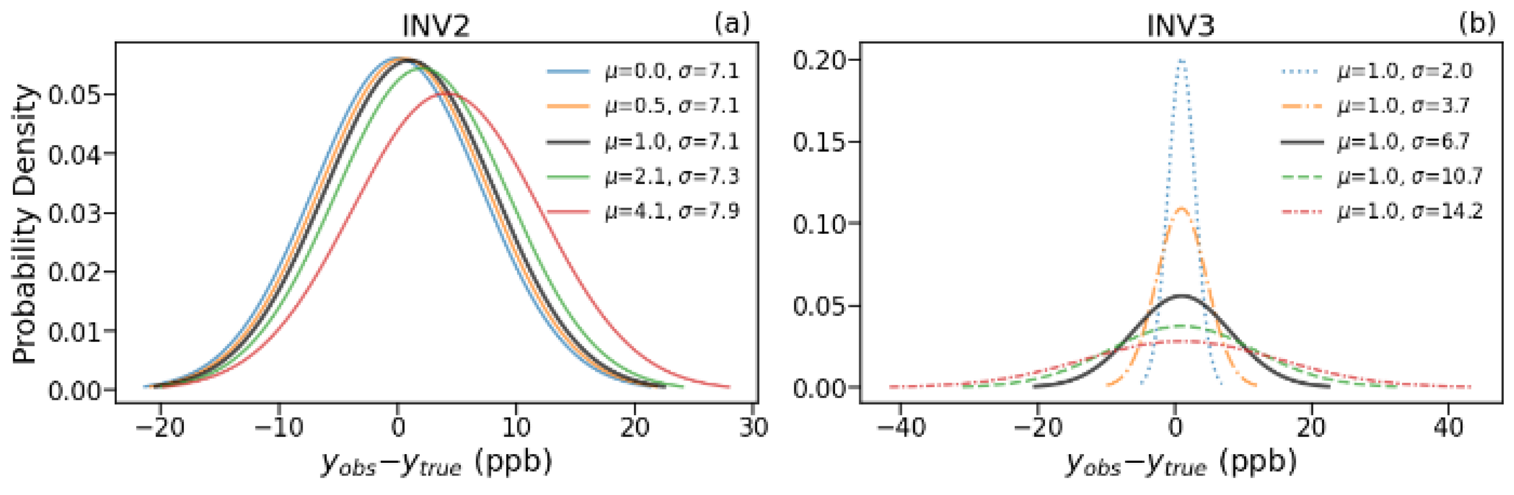
2.1.2. XCH₄ Error Scenarios

To quantify the sensitivity of the inverted CH₄ flux to $\mu$ in XCH₄ retrievals, we generated four global $\mu$ scenarios by applying factors of 0.0, 0.5, 2.0, and 4.0 to the median $\mu$ value of 1.0 ± 0.9 ppb in INV_CTL (Figure 2a). Specifically, an ideal scenario with no bias was assumed and denoted as the perfect calibration case (INV2_no_bias). The other scenarios include low (0.5 ± 0.5 ppb), high (2.1 ± 1.8 ppb), and extremely high bias (4.1 ± 3.6 ppb), respectively (Table 2). The ${\mathit{y}}^{\mathit{\prime }}$ values sampled to match valid TCCON recordings in 2017 are shown in Table S1.

The global $\sigma$ levels were adjusted using scaling factors ranging from 0.25 to 2.0 to meet different precision requirements, as evaluated in the INV3 test. This adjustment results in ${\mathit{y}}_{\mathit{o}\mathit{b}\mathit{s}}$ have biases of 1.0 ± 2.0, 1.0 ± 3.7, 1.0 ± 10.7, and 1.0 ± 14.2 ppb compared to ${\mathit{y}}_{\mathit{t}\mathit{r}\mathit{u}\mathit{e}}$, as shown in Figure 2b.

2.1.3. Large-Swath Orbits and Tansat-2 Elliptical Orbit

Currently, satellites in operation, such as GOSAT1/2, have a swath width of less than 1000 km and a spatial resolution of approximately 10 km per pixel [7,8]. The S5p-TROPOMI, with a pixel resolution of 7 km × 5.5 km, has a swath width of 2600 km [15]. All these satellites operate in a sun-synchronous orbit. At the experimental stage of this study, TanSat-2 is planned for an elliptical medium Earth orbit (MEO) with a swath width of 1500 km and a pixel size of 2 km × 2 km (Figure 3d and Table S1). Equipped with a hyperspectral grading spectrometer, TanSat-2 will cover multiple spectral bands, including the O₂-A band (0.747–0.777 μm), O₂-B band (0.672–0.702 μm), the CO₂ weak band (1.590–1.620 μm), the CH₄ band (1.63–1.67 μm), and the CO₂ strong band (1.990–2.095 μm), as well as an ultraviolet–visible band (0.4–0.5 μm) for NO₂ measurement. In this study, we assume the same pixel size of 2 km × 2 km to evaluate the performance of XCH₄ measurements with swath widths of 500 km, 1000 km, and 3000 km under a sun-synchronous orbit (Figure 3a–c) in INV4. Additionally, the performance of TanSat-2 mission is assessed in INV5.

2.2. Observation System Simulation Experiments

The XCH₄ OSSEs framework used in this study is illustrated in Figure 4. The observation operator ($\mathit{H}$) is composed of three key components: transport, sampling, and integration. For the transport process (${\mathit{H}}_{transport}$), we utilized the GEOS-Chem [45] (v12.5.0, http://www.geos-chem.org (accessed on 13 November 2019)) to establish the relationship between surface fluxes and 3D atmospheric CH₄ fields. GEOS-Chem driven by MERRA-2 meteorological re-analysis fields from the Global Modeling and Assimilation Office of NASA [46]. The “true” flux (${\mathit{X}}^t$) includes emissions from the coil mining, oil, and gas industries, livestock, rice, landfills, biomass burning, and wetland, with detailed descriptions provided in Zhu et al. (2022) [47]. Subsequently, the CH₄ fields were sampled to 2D vertical profiles based on satellite scene positions (${\mathit{H}}_{sampling}$). Finally, we integrated CH₄ profiles to column-averaged concentration XCH₄ (${\mathit{H}}_{integration}$) using GOSAT climatological average kernels [43]. The pseudo-XCH₄ retrievals ${\mathit{y}}_{\mathit{o}\mathit{b}\mathit{s}}$ were then generated based using Formula (1), as described in the previous section.

We enlarge the “true” fluxes by 80% to create the a priori fluxes (${\mathit{X}}^f=1.8 {\mathit{X}}^t$), with 70% flux errors, which we used to generate model simulations ($\mathit{H}\left({\mathit{X}}^f\right)$) [48]. The a posteriori CH₄ flux$( {\mathit{X}}^a$) and the a posteriori error covariance (${\mathit{P}}^a$) are calculated using difference between ${\mathit{y}}_{\mathit{o}\mathit{b}\mathit{s}}$ and $\mathit{H}\left({\mathit{X}}^f\right)$, as well as their uncertainties using the EnKF method [47,48,49]:

$${\mathit{X}}^a={\mathit{X}}^f+\mathit{K}\left({\mathit{y}}_{obs}-\mathit{H}\left({\mathit{X}}^f\right)\right)$$

(2)

$$\mathit{K}={\mathit{P}}^f{\mathit{H}}^T{\left(\mathit{H}{\mathit{P}}^f{\mathit{H}}^T+\mathit{R}\right)}^{-1}$$

(3)

$${\mathit{P}}^a=\left(\mathit{I}-\mathit{K}\mathit{H}\right){\mathit{P}}^f$$

(4)

For the a priori error covariance matrix (${\mathit{P}}^f$), we introduce an ensemble of perturbation states $\Delta {\mathit{X}}^f=\left[\Delta c_1^f, \Delta c_2^f, \dots ,\Delta c_{ne}^f \right]$ to approximate ${\mathit{P}}^f$ (${\mathit{P}}^f\approx \Delta {\mathit{X}}^f{(\Delta {\mathit{X}}^f)}^{\mathit{T}}$). Spatial correlations are incorporated using an exponentially decaying function based on the distance between emission grids, with a correlation length of 500 km. The sub-regions for the perturbed emissions are defined based on 11 TransCom-3 land regions [50] and are shown in Figure S2a. The temporal resolution is one week, and a lag window of four weeks is applied in the INV_CTL test.

The $\mathit{R}$ matrix accounts for all errors in mismatches between measurements and simulations, including both measurements and model errors. In our OSSEs, we focus exclusively on XCH₄ measurements errors, assuming no model errors. Moreover,$\mu$ in ${\mathit{y}}_{\mathit{o}\mathit{b}\mathit{s}}$ can theoretically be corrected through post-processing and calibration adjustments prior to inversion. Therefore, random error $\sigma$ is considered as $\mathit{R}$. The analysis was conducted during the year 2017, though all inversion tests span from October 2016 to April 2018 to mitigate edge effects.

We defined the relative error ($Fc$) to quantify the accuracy of the a posteriori estimates as follows:

$$Fc={\displaystyle \frac{\left|{\mathit{X}}^a-{\mathit{X}}^t\right|}{{\mathit{X}}^t}}\times 100\%$$

(5)

An error reduction metric ($\gamma$) is used to evaluate the improvement in uncertainty between the a priori and a posteriori fluxes.

$$\gamma =1-{\displaystyle \frac{{\mathsf{\sigma }}^a}{{\mathsf{\sigma }}^f}}$$

(6)

Here, ${\mathsf{\sigma }}^f$ and ${\mathsf{\sigma }}^a$ denote the variances of the a priori and a posteriori estimates, corresponding to the diagonal elements of the error covariance matrices ${\mathit{P}}^f$ and ${\mathit{P}}^a$, respectively. A higher $\gamma$ value indicates a greater reduction in the uncertainty of CH₄ emissions achieved through the assimilation of satellite data.

3. Results

3.1. Control Experiment

In the INV_CTL test, the globally inverted CH₄ emission achieves an accuracy of 5.1 ± 1.7% (mean ± standard deviation) relative to the “true” state (Figure 5 and Figure S3), with 86.6 ± 11.2% of the a priori uncertainties reduced. Results over the mid-latitudes (30–60°) show improved performance compared to other latitudes, achieving an $Fc$ of 1.9 ± 1.6% and a $\gamma$ of 0.7 ± 0.1. Across the 11 sub-continental regions defined in the TransCom-3 experiment [50] (Figure S2b), we found the $Fc$ values, excluding Australia, range from 3.8% to 21.6% (Figure S4).

3.2. Monthly and Weekly a Posteriori Flux Estimates

When compared to the monthly inversion results in the INV1_mon test, we found that increasing the temporal resolution improved accuracy across most regions (Figure 6). The most notable enhancement occurred in tropical South America, where $Fc$ dropped by 11.8% (INV_CTL: 1.5%; INV1_mon: 13.3%). A similar improvement was observed in temperate North America, where $Fc$ decreased from 9.6% in INV1_mon to 0.8% in INV_CTL. In temperate Eurasia, the inverted CH₄ flux exhibited consistently high accuracy in both INV1_mon (3.2%) and INV_CTL (4.2%) tests.

Over the northern hemisphere (NH), at high latitudes, the accuracy of weekly a posteriori results improved by 0.6%, 10.0%, and 4.9% in boreal North America, Europe, and boreal Eurasia, respectively, compared to their monthly results. However, in North Africa and South Africa, increasing the temporal resolution reduced inversion accuracy, likely due to the limited availability of high-quality XCH₄ observations (Figure S5). In Australia, the inversion results remained unreliable even at the monthly scale, reflecting challenges associated with detecting low CH₄ emissions.

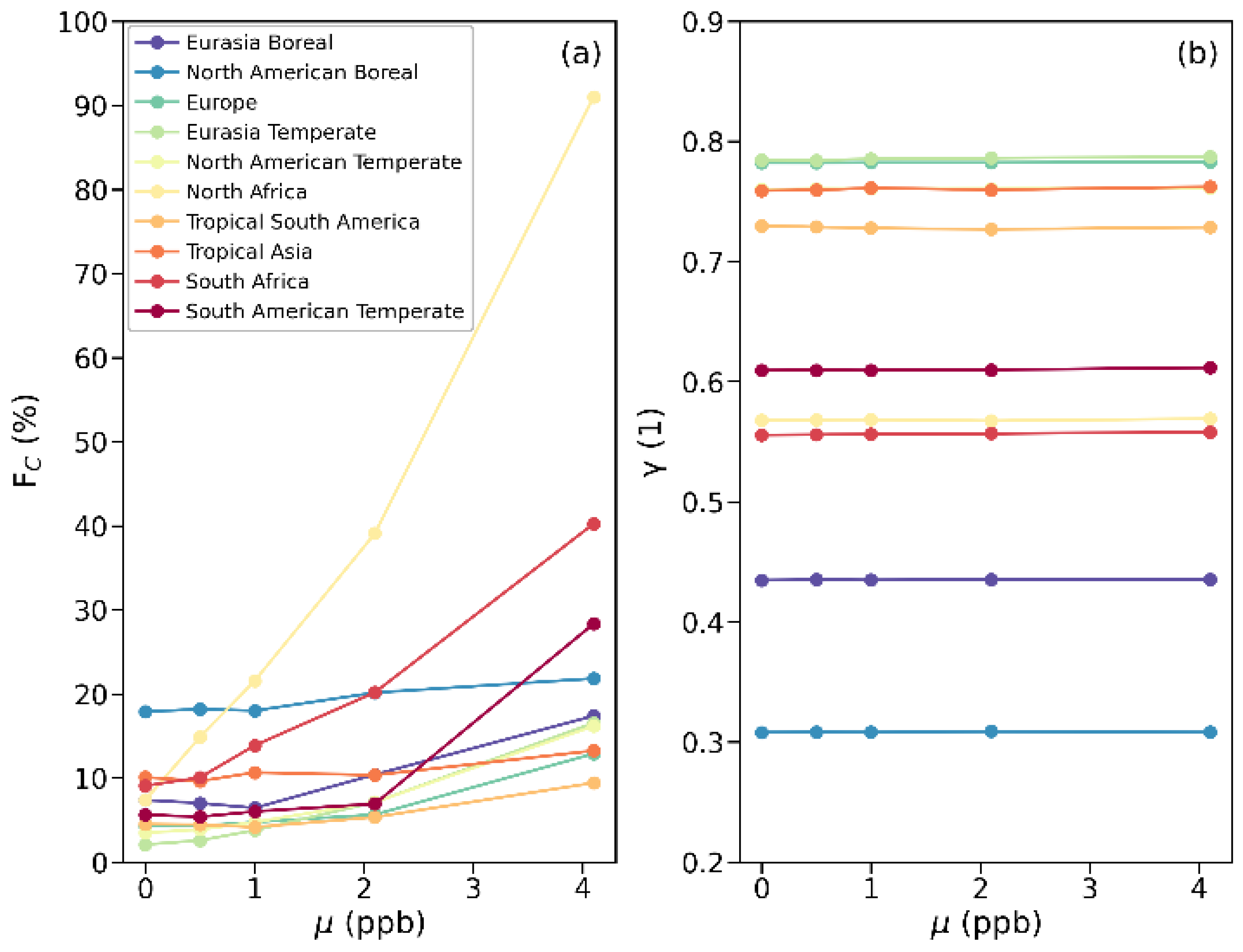
3.3. Sensitivity of a Posteriori Flux Estimates to Systematic Errors

In the INV2 test, we evaluated five bias scenarios, with $\mu$ being 0.0 ± 0.0, 0.5 ± 0.5, 1.0 ± 0.9, 2.1 ± 1.8, and 4.1 ± 3.6 ppb, and analyzed the variations in $Fc$ and $\gamma$ (Figure 7). Under the ideal condition of no bias ($\mu$ = 0.0 ± 0.0 ppb), the global total inverted CH₄ emissions achieved an accuracy of 3.4%. The temperate Eurasia and temperate North America regions exhibited the highest levels of accuracy, with $Fc$ values of 2.1% and 3.5%, respectively. Except for the boreal North America and Australia regions, all other regions achieved accuracies within 10%. When the $\mu$ values increase by a level of 4.2 ± 3.6 ppb, discrepancies exceeding 10% were observed in most regions except for tropical South America. At this extreme bias level, the global total estimate showed a 12.9% discrepancy relative to the “true” state.

In North Africa, biases are 2.7 times the global mean, with $\mu$ values as high as 10.5 ± 2.5 ppb under the extreme bias scenario. This rendered the inverted flux highly unreliable (Fc > 90%). The accuracy declines by 20.4% for every 1 ppb increase in the global $\mu$ levels. Previous studies identified significant differences of over 20 ppb between TROPOMI and GOSAT across North Africa [31,32]. Our results suggest that these discrepancies may stem not only from TROPOMI’s albedo issues but also from XCH₄ biases associated with the impact of clouds and aerosols.

In temperate South American, the $Fc$ remained below 7% for global $\mu$ levels less than 2.1 ± 1.8 ppb but increased dramatically to 28.3% when it increased by 4.1 ± 3.6 ppb. The slope of Fc to bias higher 2.1 ± 1.8 ppb are 17 times of those below 2.1 ± 1.8 ppb. The error in a posteriori CH₄ flux is independent of $\mu$ levels, with lower $\gamma$ values across high-latitudes regions due to data unavailability during the cold season (Figure 7b).

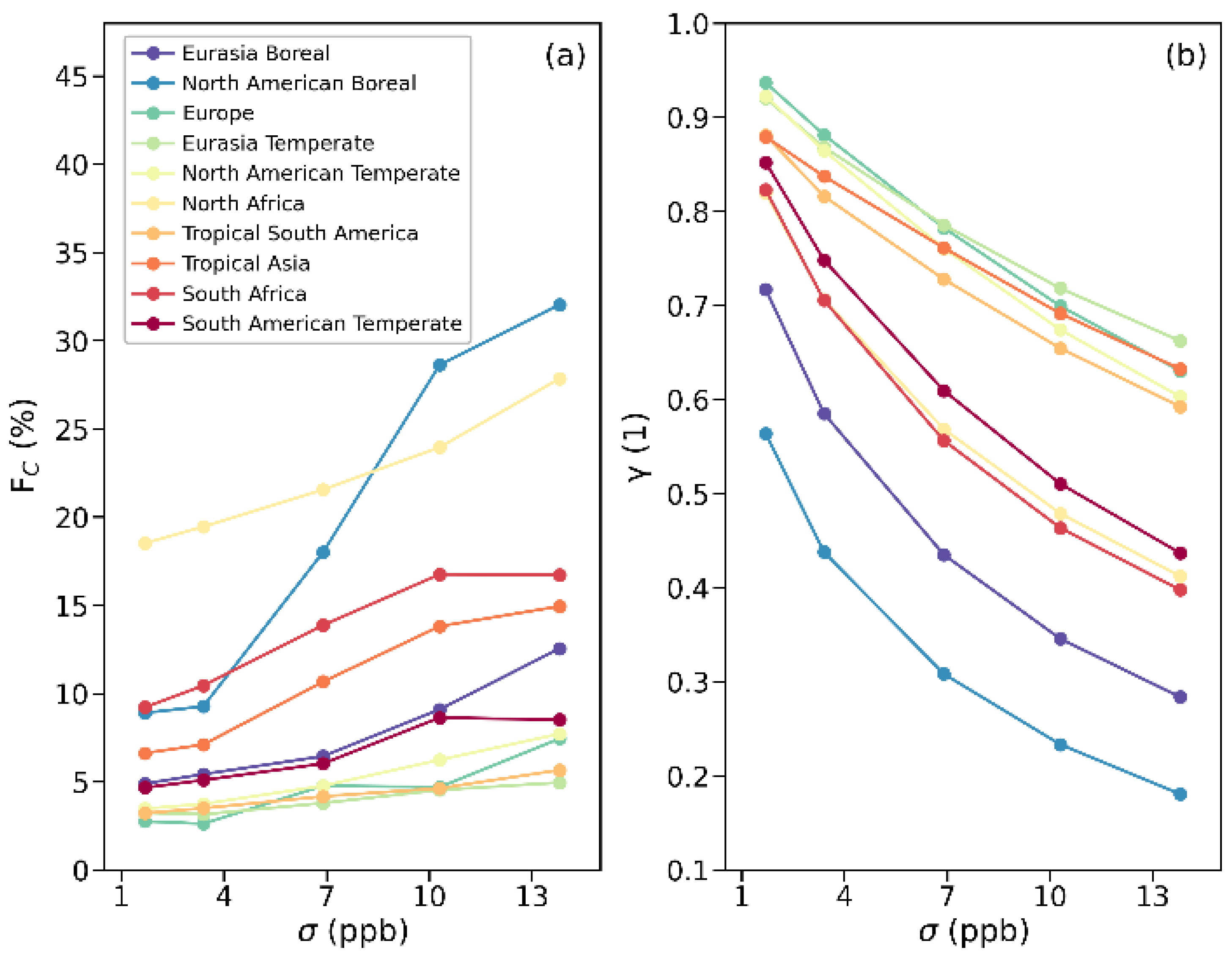
3.4. Sensitivity of Inverted Fluxes to Random Errors

Figure 8 depicts the $Fc$ and $\gamma$ variation with global $\sigma$ levels based on the setup in INV3 test. The accuracy and precision of a posteriori CH₄ flux estimates decrease as $\sigma$ increase across all regions. The boreal North American region exhibits the highest sensitivity, with $Fc$ increasing by 2.1% and $\gamma$ decreasing by 3.0% for every 1 ppb in global $\sigma$ levels. Under an extreme scenario, where $\sigma$ levels are 13.8 ± 3.2 ppb, the inverted fluxes deviate from the “true” state by 32.0%, with only 18.1% a priori uncertainties reduced. The $\sigma$ levels are less than half the precision threshold of 34 ppb proposed by Dils et al. (2014) [41] and Buchwitz et al. (2015) [35], suggesting that weekly inversion requires satellite observations with higher precision.

In North Africa, where biases are higher than in other regions, the a posteriori results show an 18.5% discrepancy from the “true” state, even under a low $\sigma$ scenario of 1.7 ± 0.4 ppb. This divergence increases to 27.8% under the extreme $\sigma$ scenario. In contrast, the inverted CH₄ fluxes in Europe, temperate Eurasia, temperate North America, and tropical South America demonstrate greater reliability, with $Fc$ values below 8% and $\gamma$ exceeding 0.6 under various $\sigma$ scenarios. We found that these regions also exhibit higher accuracy under varying $\mu$ levels, indicating that satellite observations with a swath width of 1000 km can provide sufficient and high-quality information for these areas.

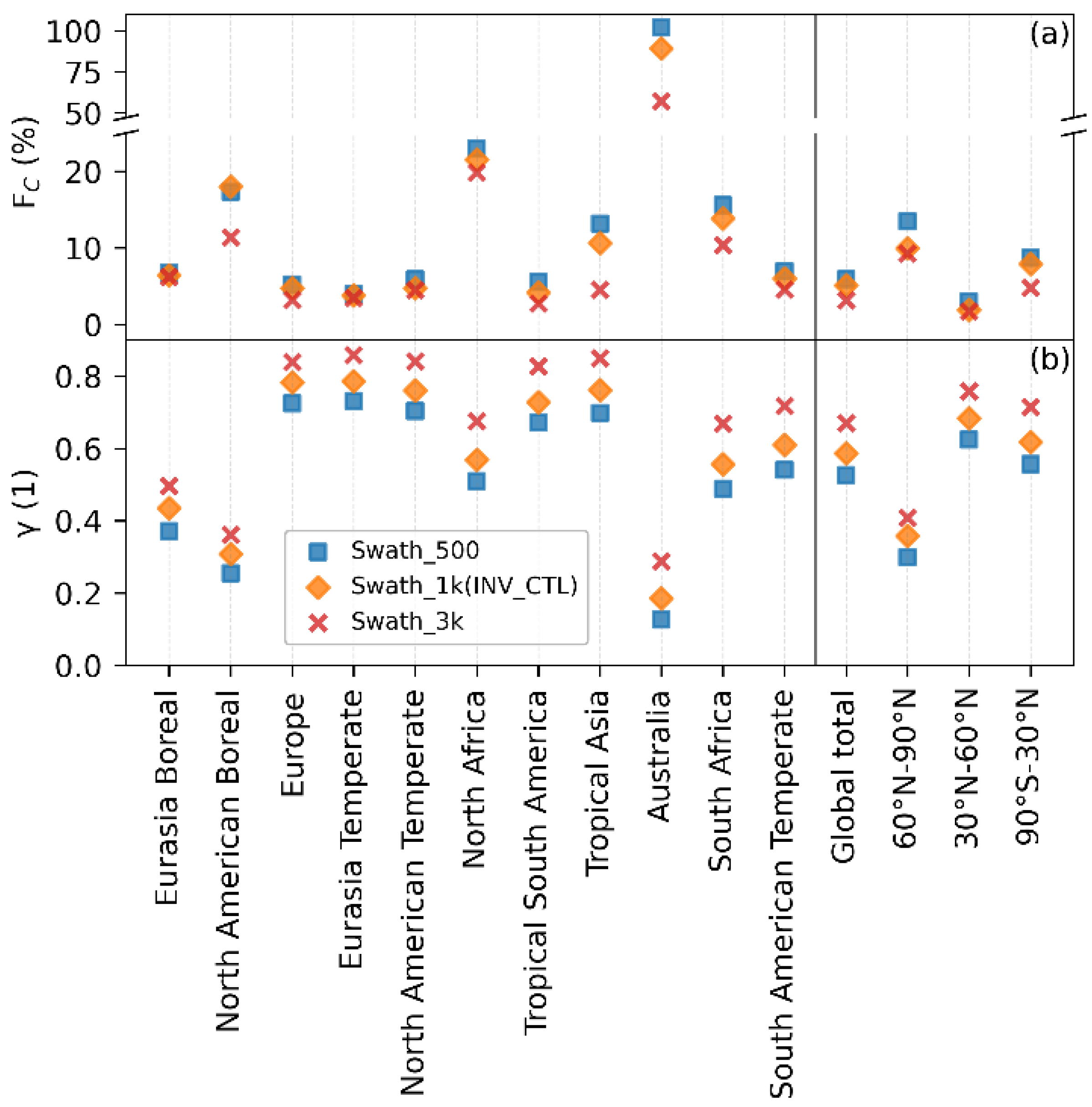
3.5. Sensitivity of Inverted Fluxes to Swath Width

In the INV4 test, we assess the impact of XCH₄ spatial coverage by comparing satellite swaths of 500 km (Swath_500) and 3000 km (Swath_3k) to the 1000 km swath used in INV_CTL (Figure 3a–c). We found that increasing satellite swath generally enhances the accuracy of inverted fluxes and reduces uncertainties across all regions. Under a scenario with $\mu$ = 1.0 ± 0.9 ppb and $\sigma$ = 6.9 ± 1.6 ppb, the global $Fc$ values are 5.9%, 5.1%, and 3.2% for the Swath_500, INV_CTL, and Swath_3k tests, respectively (Figure 9).

In regions with higher accuracy under varying $\mu$ and $\sigma$ levels, such as temperate ($Fc$ = 3.8%) Eurasia and temperate North America ($Fc$ = 5.0%), the $Fc$ values are resilient to changes in swath widths, consistent with the findings of Feng et al. (2009) [48]. In the boreal North American region, the most $\sigma$-sensitive region (Figure 8), $Fc$ in the Swath_3k test, decreased to 11.4%, compared to approximately 18% in the Swath_500 and INV_CTL tests. A similar improvement is observed in tropical Asia, another $\sigma$-sensitive region. However, for $\mu$-sensitive regions like North Africa (Figure 7), enhanced spatial coverage provides limited improvement for its a posteriori flux accuracy. In Australia, although significant improvements are observed in the Swath_3k test, discrepancies in the inverted flux still exceed 50%, accompanied by large uncertainties.

To summarize, the accuracy of inverted flux in boreal and tropical regions exhibit greater sensitivity to swath width as these regions suffer from a lower number of high-quality samples compared to the NH mid-latitudes.

3.6. Elliptical Medium Earth Orbit for TanSat-2

In the INV5 test, we compared the performance of TanSat-2 configured with elliptical orbits with a swath width of 1500 km to the INV_CTL results, which were based on sun-synchronous orbits with a swath width of 1000 km (Figure 10). The global total CH₄ flux, inverted using the TanSat-2 configuration, achieved an accuracy of 3.1 ± 2.2%, slightly outperforming the INV_CTL test. At the sub-continental scale, the discrepancies between regional inverted CH₄ fluxes and the “true” flux were 2.9 ± 3.6% higher than those observed in INV_CTL.

We attribute these discrepancies primarily to the ~13% reduction in the number of observations under the elliptical MEO compared to that in INV_CTL. For example, there was almost no coverage over the temperate North American region on 1 July 2017 due to the asymmetrical and skewed coverage pattern of the elliptical orbit (Figure 3d). Another contributing factor is the higher bias in pseudo-XCH₄ observations under the TanSat-2 configuration, which was 1.5 ± 7.1 ppb, compared to 1.0 ± 7.1 ppb in INV_CTL (Table 2). Despite this, the finer 2 km × 2 km pixel resolution of TanSat-2 offers advantages for detecting point sources (e.g., super-emitters such as coal mines and gas fields) and for performing finer regional or city-scale emission inversions [51]. At the global and sub-continental scales, we propose enhancing the swath width or adopting a dual-satellite configuration to improve inversion performance.

4. Discussion

Accurately quantifying methane emissions is a prerequisite for effective mitigation, particularly at regional scales where discrepancies are more pronounced than global estimates [11,29]. Even small biases—especially those that are spatially variable—in satellite retrievals can significantly affect the accuracy of flux inversions. For instance, when comparing the TROPOMI and GOSAT XCH₄ products, the standard deviation of their differences reaches 9–17 ppb (Table S1), leading to inconsistencies in regional CH₄ flux estimates [32]. While albedo-related biases have been identified for TROPOMI, aerosols and clouds are also critical factors contributing to these discrepancies. Assuming a linear relationship between XCH₄ bias and the total optical depth of aerosols and clouds, we conducted inversion tests across five bias scenarios (0.0 ± 0.0 to 4.1 ± 3.6 ppb; INV2). Our results show that global inverted CH₄ flux discrepancies increase by ~2.3% (~11 TgCH₄ yr⁻¹) per ppb, with regional accuracies ranging from 3.8% to 21.6% across TransCom sub-continental regions. We suggest increasing the information content on aerosol properties, through improvements in spectral resolution, signal-to-noise ratio (e.g., TanSat-2), and coordinated aerosol measurements (e.g., MAP onboard CO2M), to mitigate biases induced by multi-scattering effects.

When sampling global bias scenarios at valid TCCON recordings, the mean bias closely matches the global mean values (Table S1), thereby confirming the reliability ofth global bias correction method applied to raw satellite observations. However, the relative bias sampled at TCCON sites (0.8–2.3 ppb) is significantly underestimated compared to the global scale (7.1–7.9 ppb). Previous studies reported that the relative bias for GOSAT ranged from 2.7 to 6.0 ppb, with proxy methods yielding biases below 4 ppb. For TROPOMI, the relative bias reached 9.5 ppb, which was reduced to 4.4–6.7 ppb after correction (Table 1) but with a different spatial pattern (Figure S6). Our findings suggest that evaluations of GOSAT and TROPOMI using TCCON data may be overly optimistic. We recommend expanding validation across diverse environments to enhance the robustness of satellite XCH₄ retrievals for current and future missions.

Random errors in satellite measurements directly impact the precision of inverted CH₄ fluxes. These errors can be mitigated by increasing observation density, either through wider orbit swaths or by integrating data from multiple satellite products [31,42]. Our results show that expanding the swath width from 1000 km to 3000 km enhances flux accuracy in σ-sensitive regions (e.g., boreal North American). However, this improvement is limited in μ-sensitive regions. Given the growing availability of remote sensing data and the critical role of retrieval bias, we recommend prioritizing instrument accuracy improvements over expanding observation coverage within a fixed budget.

Tropical regions are major sources of CH₄ emissions, with a pronounced upward trend being observed in recent years [2,12,52,53,54]. However, persistent cloud cover and widespread aerosols often hinder SWIR backscattered sunlight observations, emphasizing the need for alternative orbits and ground-based measurements [55,56]. The LUCCN system, a newly developed ground-based UAV-coordinated network less affected by cloud cover, shows promise for monitoring finer regions and point sources [57,58]. At high latitudes, particularly over permafrost areas, site measurementss have identified a growing trend in CH₄ emissions, highlighting significant emission potentials under amplified warming [59,60]. These findings underscore the necessity for enhanced observational efforts, such as the pre-launch MERLIN mission, as well as the development of effective data integration techniques to harmonize measurements from various observation platforms [31,42].

In actual inversions, observation errors extended beyond the instrument errors evaluated here, including uncertainties in the observation operator, which interpret fluxes into concentrations through the transport model. In this study, only errors associated with aerosols and clouds are considered, while additional atmospheric factors that could potentially influence the results are not addressed. These additional uncertainties may degrade the performance of satellite measurements when applied to real data. It is important to emphasize that various inversion configurations could also impact the result though this aspect falls beyond the scope of this study. Thus, a comprehensive assessment of both measurement and modeling errors will be crucial in future studies.

5. Conclusions

We conducted a series of OSSEs using a GEOS-Chem + EnKF-based inversion framework to evaluate the potential of XCH₄ detection by upcoming large-swath satellites (e.g., TanSat-2) for weekly CH₄ flux inversions. Our scene-dependent analysis incorporated spatiotemporal variations in systematic ($\mu$) and random ($\sigma$) XCH₄ errors, informed by aerosol and cloud cover data from MERRA-2 reanalysis. In the INV_CTL test, with median errors ($\mu$ = 1.0 ± 0.9 ppb and $\sigma$ = 6.9 ± 1.6 ppb) over a 1000 km swath on sun-synchronous orbits, the global inverted CH₄ flux achieved an accuracy of 5.1 ± 1.7%, reducing a priori uncertainties by 86.6 ± 11.2%. We identified relationships between inverted CH₄ flux accuracy/precision and global $\mu$ and $\sigma$ levels, finding robust results in NH mid-latitudes but greater sensitivity in tropical and boreal regions due to limited high-quality observations. Inverted results in boreal regions exhibit higher sensitivity to $\sigma$, primarily due to limited observational coverage. In contrast, measurements in the tropical regions are more susceptible to biases, which further compromises the accuracy of the inverted fluxes. Therefore, expanding swath width mitigates discrepancies in $\sigma$-sensitive regions, while $\mu$-sensitive regions require alternative improvement strategies. For TanSat-2 in an elliptical orbit, global total estimates achieved an accuracy of 3.1 ± 2.2%. Our analysis highlights key links between various satellite configurations and precision thresholds for emission estimates, offering valuable guidance for upcoming XCH₄ satellite missions such as GOSAT-GW, Sentinel-5, and CO2M.

References

1. Peng, S.; Lin, X.; Thompson, R.L.; Xi, Y.; Liu, G.; Hauglustaine, D.; Lan, X.; Poulter, B.; Ramonet, M.; Saunois, M.; et al. Wetland Emission and Atmospheric Sink Changes Explain Methane Growth in 2020. Nature 2022, 612, 477–482. [Google Scholar] [CrossRef]
2. Feng, L.; Palmer, P.I.; Parker, R.J.; Lunt, M.F.; Bösch, H. Methane Emissions Are Predominantly Responsible for Record-Breaking Atmospheric Methane Growth Rates in 2020 and 2021. Atmos. Chem. Phys. 2023, 23, 4863–4880. [Google Scholar] [CrossRef]
3. Palmer, P.I.; Feng, L.; Lunt, M.F.; Parker, R.J.; Bösch, H.; Lan, X.; Lorente, A.; Borsdorff, T. The Added Value of Satellite Observations of Methane Forunderstanding the Contemporary Methane Budget. Philos. Trans. R. Soc. A Math. Phys. Eng. Sci. 2021, 379, 20210106. [Google Scholar] [CrossRef]
4. Jacob, D.J.; Varon, D.J.; Cusworth, D.H.; Dennison, P.E.; Frankenberg, C.; Gautam, R.; Guanter, L.; Kelley, J.; McKeever, J.; Ott, L.E.; et al. Quantifying Methane Emissions from the Global Scale down to Point Sources Using Satellite Observations of Atmospheric Methane. Atmos. Chem. Phys. 2022, 22, 9617–9646. [Google Scholar] [CrossRef]
5. UNEP. United Nations Environment Programme/Climate and Clean Air Coalition. Global Methane Assessment: 2030 Baseline Report; UNEP: Nariobi, Kenya, 2022. [Google Scholar]
6. Bovensmann, H.; Burrows, J.P.; Buchwitz, M.; Frerick, J.; Noël, S.; Rozanov, V.V.; Chance, K.V.; Goede, A.P.H. SCIAMACHY: Mission Objectives and Measurement Modes. J. Atmos. Sci. 1999, 56, 127–150. [Google Scholar] [CrossRef]
7. Yokota, T.; Yoshida, Y.; Eguchi, N.; Ota, Y.; Tanaka, T.; Watanabe, H.; Maksyutov, S. Global Concentrations of CO2 and CH4 Retrieved from GOSAT: First Preliminary Results. Sola 2009, 5, 160–163. [Google Scholar] [CrossRef]
8. Imasu, R.; Matsunaga, T.; Nakajima, M.; Yoshida, Y.; Shiomi, K.; Morino, I.; Saitoh, N.; Niwa, Y.; Someya, Y.; Oishi, Y.; et al. Greenhouse Gases Observing SATellite 2 (GOSAT-2): Mission Overview. Prog. Earth Planet. Sci. 2023, 10, 33. [Google Scholar] [CrossRef]
9. Lu, X.; Jacob, D.J.; Zhang, Y.; Maasakkers, J.D.; Sulprizio, M.P.; Shen, L.; Qu, Z.; Scarpelli, T.R.; Nesser, H.; Yantosca, R.M.; et al. Global Methane Budget and Trend, 2010–2017: Complementarity of Inverse Analyses Using in Situ (GLOBALVIEWplus CH4 ObsPack) and Satellite (GOSAT) Observations. Atmos. Chem. Phys. 2021, 21, 4637–4657. [Google Scholar] [CrossRef]
10. Qu, Z.; Jacob, D.J.; Bloom, A.A.; Worden, J.R.; Parker, R.J.; Boesch, H. Inverse Modeling of 2010–2022 Satellite Observations Shows That Inundation of the Wet Tropics Drove the 2020–2022 Methane Surge. Proc. Natl. Acad. Sci. USA 2024, 121, e2402730121. [Google Scholar] [CrossRef] [PubMed]
11. Stavert, A.; Saunois, M.; Canadell, J.; Poulter, B.; Jackson, R.; Regnier, P.; Lauerwald, R.; Raymond, P.; Allen, G.; Patra, P.; et al. Regional Trends and Drivers of the Global Methane Budget. Glob. Chang. Biol. 2022, 28, 182–200. [Google Scholar] [CrossRef]
12. Yin, Y.; Chevallier, F.; Ciais, P.; Bousquet, P.; Saunois, M.; Zheng, B.; Worden, J.; Bloom, A.A.; Parker, R.J.; Jacob, D.J.; et al. Accelerating Methane Growth Rate from 2010 to 2017: Leading Contributions from the Tropics and East Asia. Atmos. Chem. Phys. 2021, 21, 12631–12647. [Google Scholar] [CrossRef]
13. Zhang, Y.; Jacob, D.J.; Lu, X.; Maasakkers, J.D.; Scarpelli, T.R.; Sheng, J.-X.; Shen, L.; Qu, Z.; Sulprizio, M.P.; Chang, J.; et al. Attribution of the Accelerating Increase in Atmospheric Methane during 2010–2018 by Inverse Analysis of GOSAT Observations. Atmos. Chem. Phys. 2021, 21, 3643–3666. [Google Scholar] [CrossRef]
14. Feng, L.; Palmer, P.I.; Zhu, S.; Parker, R.J.; Liu, Y. Tropical Methane Emissions Explain Large Fraction of Recent Changes in Global Atmospheric Methane Growth Rate. Nat. Commun. 2022, 13, 1378. [Google Scholar] [CrossRef]
15. Lorente, A.; Borsdorff, T.; Butz, A.; Hasekamp, O.; aan de Brugh, J.; Schneider, A.; Wu, L.; Hase, F.; Kivi, R.; Wunch, D.; et al. Methane Retrieved from TROPOMI: Improvement of the Data Product and Validation of the First 2 Years of Measurements. Atmos. Meas. Tech. 2021, 14, 665–684. [Google Scholar] [CrossRef]
16. Gao, M.; Xing, Z.; Vollrath, C.; Hugenholtz, C.H.; Barchyn, T.E. Global Observational Coverage of Onshore Oil and Gas Methane Sources with TROPOMI. Sci. Rep. 2023, 13, 16759. [Google Scholar] [CrossRef] [PubMed]
17. Shen, L.; Jacob, D.J.; Gautam, R.; Omara, M.; Scarpelli, T.R.; Lorente, A.; Zavala-Araiza, D.; Lu, X.; Chen, Z.; Lin, J. National Quantifications of Methane Emissions from Fuel Exploitation Using High Resolution Inversions of Satellite Observations. Nat. Commun. 2023, 14, 4948. [Google Scholar] [CrossRef] [PubMed]
18. Zhang, Y.; Gautam, R.; Pandey, S.; Omara, M.; Maasakkers, J.D.; Sadavarte, P.; Lyon, D.; Nesser, H.; Sulprizio, M.P.; Varon, D.J.; et al. Quantifying Methane Emissions from the Largest Oil-Producing Basin in the United States from Space. Sci. Adv. 2020, 6, eaaz5120. [Google Scholar] [CrossRef] [PubMed]
19. Nesser, H.; Jacob, D.J.; Maasakkers, J.D.; Lorente, A.; Chen, Z.; Lu, X.; Shen, L.; Qu, Z.; Sulprizio, M.P.; Winter, M.; et al. High-Resolution US Methane Emissions Inferred from an Inversion of 2019 TROPOMI Satellite Data: Contributions from Individual States, Urban Areas, and Landfills. Atmos. Chem. Phys. 2024, 24, 5069–5091. [Google Scholar] [CrossRef]
20. Hamburg, S.; Gautam, R.; Zavala-Araiza, D. MethaneSAT—A New Tool Purpose-Built to Measure Oil and Gas Methane Emissions from Space. In Proceedings of the Abu Dhabi International Petroleum Exhibition and Conference, Abu Dhabi, United Arab Emirates, 31 October 2022; SPE: Abu Dhabi, United Arab Emirates, 2022; p. D011S007R002. [Google Scholar]
21. Liu, Y.; Wang, J.; Yao, L.; Chen, X.; Cai, Z.; Yang, D.; Yin, Z.; Gu, S.; Tian, L.; Lu, N.; et al. The TanSat Mission: Preliminary Global Observations. Sci. Bull. 2018, 63, 1200–1207. [Google Scholar] [CrossRef]
22. Yang, D.; Liu, Y.; Cai, Z.; Chen, X.; Yao, L.; Lu, D. First Global Carbon Dioxide Maps Produced from TanSat Measurements. Adv. Atmos. Sci. 2018, 35, 621–623. [Google Scholar] [CrossRef]
23. Ran, Y. TanSat: A New Star in Global Carbon Monitoring from China. Sci. Bull. 2019, 64, 284–285. [Google Scholar] [CrossRef] [PubMed]
24. Yang, D.; Boesch, H.; Liu, Y.; Somkuti, P.; Cai, Z.; Chen, X.; Di Noia, A.; Lin, C.; Lu, N.; Lyu, D.; et al. Toward High Precision XCO2 Retrievals From TanSat Observations: Retrieval Improvement and Validation Against TCCON Measurements. J. Geophys. Res. Atmos. 2020, 125, e2020JD032794. [Google Scholar] [CrossRef] [PubMed]
25. Yang, D.; Liu, Y.; Boesch, H.; Yao, L.; Di Noia, A.; Cai, Z.; Lu, N.; Lyu, D.; Wang, M.; Wang, J.; et al. A New TanSat XCO2 Global Product towards Climate Studies. Adv. Atmos. Sci. 2021, 38, 8–11. [Google Scholar] [CrossRef]
26. Yao, L.; Yang, D.; Liu, Y.; Wang, J.; Liu, L.; Du, S.; Cai, Z.; Lu, N.; Lyu, D.; Wang, M.; et al. A New Global Solar-Induced Chlorophyll Fluorescence (SIF) Data Product from TanSat Measurements. Adv. Atmos. Sci. 2021, 38, 341–345. [Google Scholar] [CrossRef]
27. Wang, H.; Jiang, F.; Liu, Y.; Yang, D.; Wu, M.; He, W.; Wang, J.; Wang, J.; Ju, W.; Chen, J.M. Global Terrestrial Ecosystem Carbon Flux Inferred from TanSat XCO2 Retrievals. J. Remote Sens. 2022, 2022, 9816536. [Google Scholar] [CrossRef]
28. Yang, D.; Hakkarainen, J.; Liu, Y.; Ialongo, I.; Cai, Z.; Tamminen, J. Detection of Anthropogenic CO2 Emission Signatures with TanSat CO2 and with Copernicus Sentinel-5 Precursor (S5P) NO2 Measurements: First Results. Adv. Atmos. Sci. 2023, 40, 1–5. [Google Scholar] [CrossRef] [PubMed]
29. Saunois, M.; Martinez, A.; Poulter, B.; Zhang, Z.; Raymond, P.; Regnier, P.; Canadell, J.G.; Jackson, R.B.; Patra, P.K.; Bousquet, P.; et al. Global Methane Budget 2000–2020. In Earth System Science Data Discussions; Copernicus Publications: Göttingen, Germany, 2024; pp. 1–147. [Google Scholar] [CrossRef]
30. Houweling, S.; Bergamaschi, P.; Chevallier, F.; Heimann, M.; Kaminski, T.; Krol, M.; Michalak, A.M.; Patra, P. Global Inverse Modeling of CH4 Sources and Sinks: An Overview of Methods. Atmos. Chem. Phys. 2017, 17, 235–256. [Google Scholar] [CrossRef]
31. Balasus, N.; Jacob, D.J.; Lorente, A.; Maasakkers, J.D.; Parker, R.J.; Boesch, H.; Chen, Z.; Kelp, M.M.; Nesser, H.; Varon, D.J. A Blended TROPOMI+GOSAT Satellite Data Product for Atmospheric Methane Using Machine Learning to Correct Retrieval Biases. Atmos. Meas. Tech. 2023, 16, 3787–3807. [Google Scholar] [CrossRef]
32. Qu, Z.; Jacob, D.J.; Shen, L.; Lu, X.; Zhang, Y.; Scarpelli, T.R.; Nesser, H.; Sulprizio, M.P.; Maasakkers, J.D.; Bloom, A.A.; et al. Global Distribution of Methane Emissions: A Comparative Inverse Analysis of Observations from the TROPOMI and GOSAT Satellite Instruments. Atmos. Chem. Phys. 2021, 21, 14159–14175. [Google Scholar] [CrossRef]
33. Schneising, O.; Buchwitz, M.; Hachmeister, J.; Vanselow, S.; Reuter, M.; Buschmann, M.; Bovensmann, H.; Burrows, J.P. Advances in Retrieving XCH4 and XCO from Sentinel-5 Precursor: Improvements in the Scientific TROPOMI/WFMD Algorithm. Atmos. Meas. Tech. 2023, 16, 669–694. [Google Scholar] [CrossRef]
34. Chevallier, F.; Bréon, F.; Rayner, P.J. Contribution of the Orbiting Carbon Observatory to the Estimation of CO2 Sources and Sinks: Theoretical Study in a Variational Data Assimilation Framework. J. Geophys. Res. 2007, 112, 2006JD007375. [Google Scholar] [CrossRef]
35. Buchwitz, M.; Reuter, M.; Schneising, O.; Boesch, H.; Guerlet, S.; Dils, B.; Aben, I.; Armante, R.; Bergamaschi, P.; Blumenstock, T.; et al. The Greenhouse Gas Climate Change Initiative (GHG-CCI): Comparison and Quality Assessment of near-Surface-Sensitive Satellite-Derived CO2 and CH4 Global Data Sets. Remote Sens. Environ. 2015, 162, 344–362. [Google Scholar] [CrossRef]
36. Aben, I.; Hasekamp, O.; Hartmann, W. Uncertainties in the Space-Based Measurements of CO2 Columns Due to Scattering in the Earth’s Atmosphere. J. Quant. Spectrosc. Radiat. Transf. 2007, 104, 450–459. [Google Scholar] [CrossRef]
37. Butz, A.; Hasekamp, O.P.; Frankenberg, C.; Vidot, J.; Aben, I. CH4 Retrievals from Space-based Solar Backscatter Measurements: Performance Evaluation against Simulated Aerosol and Cirrus Loaded Scenes. J. Geophys. Res. 2010, 115, 2010JD014514. [Google Scholar] [CrossRef]
38. Chander, G.; Hewison, T.J.; Fox, N.; Wu, X.; Xiong, X.; Blackwell, W.J. Overview of Intercalibration of Satellite Instruments. IEEE Trans. Geosci. Remote Sens. 2013, 51, 1056–1080. [Google Scholar] [CrossRef]
39. von Clarmann, T.; Degenstein, D.A.; Livesey, N.J.; Bender, S.; Braverman, A.; Butz, A.; Compernolle, S.; Damadeo, R.; Dueck, S.; Eriksson, P.; et al. Overview: Estimating and Reporting Uncertainties in Remotely Sensed Atmospheric Composition and Temperature. Atmos. Meas. Tech. 2020, 13, 4393–4436. [Google Scholar] [CrossRef]
40. Kiefer, M.; von Clarmann, T.; Funke, B.; García-Comas, M.; Glatthor, N.; Grabowski, U.; Kellmann, S.; Kleinert, A.; Laeng, A.; Linden, A.; et al. IMK/IAA MIPAS Temperature Retrieval Version 8: Nominal Measurements. Atmos. Meas. Tech. 2021, 14, 4111–4138. [Google Scholar] [CrossRef]
41. Dils, B.; Buchwitz, M.; Reuter, M.; Schneising, O.; Boesch, H.; Parker, R.; Guerlet, S.; Aben, I.; Blumenstock, T.; Burrows, J.P.; et al. The Greenhouse Gas Climate Change Initiative (GHG-CCI): Comparative Validation of GHG-CCI SCIAMACHY/ENVISAT and TANSO-FTS/GOSAT CO2 and CH4 Retrieval Algorithm Products with Measurements from the TCCON. Atmos. Meas. Tech. 2014, 7, 1723–1744. [Google Scholar] [CrossRef]
42. Reuter, M.; Buchwitz, M.; Schneising, O.; Noël, S.; Bovensmann, H.; Burrows, J.P.; Boesch, H.; Di Noia, A.; Anand, J.; Parker, R.J.; et al. Ensemble-Based Satellite-Derived Carbon Dioxide and Methane Column-Averaged Dry-Air Mole Fraction Data Sets (2003–2018) for Carbon and Climate Applications. Atmos. Meas. Tech. 2020, 13, 789–819. [Google Scholar] [CrossRef]
43. Parker, R.J.; Webb, A.; Boesch, H.; Somkuti, P.; Barrio Guillo, R.; Di Noia, A.; Kalaitzi, N.; Anand, J.S.; Bergamaschi, P.; Chevallier, F.; et al. A Decade of GOSAT Proxy Satellite CH4 Observations. Earth System Science Data 2020, 12, 3383–3412. [Google Scholar] [CrossRef]
44. Lorente, A.; Borsdorff, T.; Martinez-Velarte, M.C.; Landgraf, J. Accounting for Surface Reflectance Spectral Features in TROPOMI Methane Retrievals. Atmos. Meas. Tech. 2023, 16, 1597–1608. [Google Scholar] [CrossRef]
45. The International GEOS-Chem User Community Geoschem/Geos-Chem: GEOS-Chem 12.5.0 2019. Available online: https://zenodo.org/records/3403111 (accessed on 13 November 2019).
46. Gelaro, R.; McCarty, W.; Suárez, M.J.; Todling, R.; Molod, A.; Takacs, L.; Randles, C.A.; Darmenov, A.; Bosilovich, M.G.; Reichle, R.; et al. The Modern-Era Retrospective Analysis for Research and Applications, Version 2 (MERRA-2). J. Clim. 2017, 30, 5419–5454. [Google Scholar] [CrossRef] [PubMed]
47. Zhu, S.; Feng, L.; Liu, Y.; Wang, J.; Yang, D. Decadal Methane Emission Trend Inferred from Proxy GOSAT XCH4 Retrievals: Impacts of Transport Model Spatial Resolution. Adv. Atmos. Sci. 2022, 39, 1343–1359. [Google Scholar] [CrossRef]
48. Feng, L.; Palmer, P.; Boesch, H.; Dance, S. Estimating Surface CO2 Fluxes from Space-Borne CO2 Dry Air Mole Fraction Observations Using an Ensemble Kalman Filter. Atmos. Chem. Phys. 2009, 9, 2619–2633. [Google Scholar] [CrossRef]
49. Feng, L.; Palmer, P.I.; Bösch, H.; Parker, R.J.; Webb, A.J.; Correia, C.S.C.; Deutscher, N.M.; Domingues, L.G.; Feist, D.G.; Gatti, L.V.; et al. Consistent Regional Fluxes of CH4 and CO2 Inferred from GOSAT Proxy XCH4: XCO2 Retrievals, 2010–2014. Atmos. Chem. Phys. 2017, 17, 4781–4797. [Google Scholar] [CrossRef]
50. Gurney, K.; Law, R.; Denning, S.; Rayner, P.; Baker, D.; Bousquet, P.; Bruhwiler, L.; Chen, Y.-H.; Ciais, P.; Fan, S.-M.; et al. Towards Robust Regional Estimates of CO2 Sources and Sinks Using Atmospheric Transport Models. Nature 2002, 415, 626–630. [Google Scholar] [CrossRef]
51. Wu, K.; Yang, D.; Liu, Y.; Cai, Z.; Zhou, M.; Feng, L.; Palmer, P.I. Evaluating the Ability of the Pre-Launch TanSat-2 Satellite to Quantify Urban CO2 Emissions. Remote Sens. 2023, 15, 4904. [Google Scholar] [CrossRef]
52. Lunt, M.F.; Palmer, P.I.; Feng, L.; Taylor, C.M.; Boesch, H.; Parker, R.J. An Increase in Methane Emissions from Tropical Africa between 2010 and 2016 Inferred from Satellite Data. Atmos. Chem. Phys. 2019, 19, 14721–14740. [Google Scholar] [CrossRef]
53. Lunt, M.F.; Palmer, P.I.; Lorente, A.; Borsdorff, T.; Landgraf, J.; Parker, R.J.; Boesch, H. Rain-Fed Pulses of Methane from East Africa during 2018–2019 Contributed to Atmospheric Growth Rate. Environ. Res. Lett. 2021, 16, 024021. [Google Scholar] [CrossRef]
54. Zhang, Z.; Poulter, B.; Feldman, A.; Ying, Q.; Ciais, P.; Peng, S.; Li, X. Recent Intensification of Wetland Methane Feedback. Nat. Clim. Chang. 2023, 13, 430–433. [Google Scholar] [CrossRef]
55. Merbold, L.; Scholes, R.; Acosta, M.; Beck, J.; Bombelli, A.; Fiedler, B.; Grieco, E.; Helmschrot, J.; Hugo, W.; Kasurinen, V.; et al. Opportunities for an African Greenhouse Gas Observation System. Reg. Environ. Chang. 2021, 21, 104. [Google Scholar] [CrossRef]
56. Nickless, A.; Scholes, R.J.; Vermeulen, A.; Beck, J.; Lopez-Ballesteros, A.; Ardö, J.; Karstens, U.; Rigby, M.L.; Kasurinen, V.; Pantazatou, K.; et al. Greenhouse Gas Observation Network Design for Africa. Tellus B 2020, 72, 1–30. [Google Scholar] [CrossRef]
57. Yang, D.; Zhao, T.; Yao, L.; Guo, D.; Fan, M.; Ren, X.; Li, M.; Wu, K.; Wang, J.; Cai, Z.; et al. Toward Establishing a Low-Cost UAV Coordinated Carbon Observation Network (LUCCN): First Integrated Campaign in China. Adv. Atmos. Sci. 2024, 41, 1–7. [Google Scholar] [CrossRef]
58. Zhao, T.; Yang, D.; Guo, D.; Wang, Y.; Yao, L.; Ren, X.; Fan, M.; Cai, Z.; Wu, K.; Liu, Y. Low-Cost UAV Coordinated Carbon Observation Network: Carbon Dioxide Measurement with Multiple UAVs. Atmos. Environ. 2024, 332, 120609. [Google Scholar] [CrossRef]
59. Rößger, N.; Sachs, T.; Wille, C.; Boike, J.; Kutzbach, L. Seasonal Increase of Methane Emissions Linked to Warming in Siberian Tundra. Nat. Clim. Chang. 2022, 12, 1031–1036. [Google Scholar] [CrossRef]
60. Smith, S.; O’Neill, B.; Isaksen, K.; Noetzli, J.; Romanovsky, V. The Changing Thermal State of Permafrost. Nat. Rev. Earth Environ. 2022, 3, 10–23. [Google Scholar] [CrossRef]
Figure 1. Probability distribution of retravelled XCH4 systematic errors, μ (a), random errors, σ (b), and difference y between pseudo and the “true” XCH4 observation (c) on 1 July 2017.
Remotesensing 17 00543 g001
Figure 2. Probability distribution of the XCH4 increments   y added to y t r u e in INV2 tests (a) with various systematic errors ( μ = 0.0, 0.5, 1.0, 2.1, and 4.1 ppb) and in INV3 tests (b) with various random errors ( σ = 2.0, 3.7, 6.7, 10.7, and 14.2 ppb) from 1 January to 31 December 2017. The black lines in the panels (a,b) denote the scenario of INV_CTL test.
Remotesensing 17 00543 g002
Figure 3. The number of cloud- and aerosol-free scenes (AOD@550nm < 0.5) on 1 July 2017, averaged on a 2° × 2.5° (latitude × longitude) grid for sun-synchronous orbits with swath widths of 500 km (a), 1000 km (b), and 3000 km (c), as well as for the TanSat-2 elliptical MEO with a swath width of 1500 km (d) in INV4 and INV5 tests.
Remotesensing 17 00543 g003
Figure 4. Schematic of OSSEs. The left column (blue arrows) outlines the generation of pseudo-observations ( y o b s ) using the observation operator ( H ), which maps the “true” flux ( X t ) to observed XCH4. R represents observation error. The right column (green arrows) denotes the model forecast process based on the a priori estimate ( X f ), which is 80% larger than X t , along with the associated error. The middle column (black arrows) represents the iterative assimilation process based on the EnKF algorithm to generate the a posteriori estimate ( X a ) and its uncertainties ( P a ). The black boxes indicate variables, and the shaded areas denote calculation processes within the OSSEs.
Remotesensing 17 00543 g004
Figure 5. CH4 emission variations are depicted for the global total (a), regions south of 30° N (b), between 30° N and 60° N (c), and north of 60° N (d) under the INV_CTL test, incorporating median systematic and random errors (1.0 ± 7.0 ppb) in XCH4 retrievals. The blue line represents the a priori emissions, the orange line denotes the a posteriori emissions, and the black line illustrates the “true” emissions. Shaded areas around the blue and orange lines reflect the uncertainties associated with the a priori and a posteriori emissions, respectively.
Remotesensing 17 00543 g005
Figure 6. Annual CH4 emissions for 11 Transcom land regions, comparing a priori estimates (blue), weekly (orange, INV_CTL), and monthly (green, INV1_mon) a posteriori estimates, and the “true” emissions (red line) (a). The corresponding F c values from the INV_CTL (orange diamond) and INV1_mon (green cross) inversion tests are shown in panel (b).
Remotesensing 17 00543 g006
Figure 7. Accuracy and precision of the inverted CH₄ fluxes under five scenarios with varying global systematic error levels: zero ( μ = 0.0 ± 0.0 ppb), low ( μ = 0.5 ± 0.5 ppb), median ( μ = 1.0 ± 0.9 ppb), high ( μ = 2.1 ± 1.8 ppb), and extreme ( μ = 4.1 ± 3.6 ppb), as defined in the INV2 test. Panels (a,b) display the weekly weighted mean F c (%) and weekly mean γ (1) values across TransCom-3 land regions, excluding Australia.
Remotesensing 17 00543 g007
Figure 8. Accuracy and precision of the inverted CH₄ fluxes under five scenarios with varying global random error levels: low ( σ = 1.7 ± 0.4 ppb), slightly low ( σ = 3.4 ± 0.8 ppb), median ( σ = 6.9 ± 1.6 ppb), high ( σ = 10.3 ± 2.5 ppb), and extreme ( σ = 13.8 ± 3.2 ppb), as defined in the INV3 test. Panels (a,b) display the weekly weighted mean F c (%) and weekly mean γ (1) values across TransCom-3 land regions, excluding Australia.
Remotesensing 17 00543 g008
Figure 9. Accuracy and precision of the inverted CH₄ flux under satellite swaths widths of 500 km (blue square), 1000 km (orange diamond), and 3000 km (red cross), as defined in the INV4 test. Panel (a) illustrates the weighted mean F c (%) across the 11 TransCom-3 land regions, as well as global and latitudinal zones. Panel (b) presents the weekly mean γ (1) values.
Remotesensing 17 00543 g009
Figure 10. Accuracy and precision of the inverted CH₄ flux under TanSat-2 elliptical MEO with a swath width of 1500 km (green cross) and CTL_INV, configured with a swath width of 1000 km under sun-synchronous orbits (orange diamond), as defined in the INV5 test. Panel (a) illustrates the weighted mean F c (%) across the 11 TransCom-3 land regions, as well as global and latitudinal zones. Panel (b) presents the weekly mean γ (1) values.
Remotesensing 17 00543 g010