Abstract
To address the limitations of Global Navigation Satellite Systems (GNSSs), such as vulnerability to electromagnetic interference and weak ground signal power, signal of opportunity (SOP) provided by low Earth orbit (LEO) satellites can serve as a backup positioning method. By simulating a LEO constellation, the impact of satellite visibility, Doppler geometric dilution of precision (DGDOP), and positioning accuracy was explored. Considering positioning errors such as satellite clock drift rate, ionospheric delay rate, tropospheric delay rate, and Earth rotation effects, the instantaneous positioning performance with satellite orbital errors and satellite velocity errors of different magnitudes was simulated. The results show that satellite visibility and DGDOP are negatively correlated. In a typical atmospheric environment with orbital errors of 10 m and satellite velocity errors of 0.1 m/s, positioning accuracy within 30 m can be achieved. This confirms that Doppler-based positioning with LEO satellites can be used as a backup method for GNSSs.
1. Introduction
Presently, a Global Navigation Satellite System (GNSS) consisting of a Global Positioning System (GPS), Global Navigation Satellite System (GLONASS), Galileo Global Navigation Satellite System (Galileo), BeiDou Navigation Satellite System (BDS) has been established internationally [1]. However, the navigation signal from GNSS has low power when the signal reaches the Earth surface, making it susceptible to interference, obstruction, and deception during transmission. Especially in areas with severe obstructions, there may be a lack of signal or weak signal phenomenon, which makes it difficult to meet the application requirements in modern complex electromagnetic environments [2]. Low Earth orbit (LEO) satellites typically pertain to satellites that operate within an orbital altitude ranging from 300 to 1500 km. Compared with a medium earth orbit satellite, a LEO satellite has advantages in providing a reliable signal of opportunity (SOP) for positioning and navigation due to lower orbital altitude, stronger ground signal reception, larger number of satellites, wider coverage range, and stable transmission performance [3]. This positioning technique has the ability of serving as a backup solution for a GNSS.
In recent years, the advancements in “one rocket multiple satellites” launch technology and batch low-cost satellite manufacturing have led to the emergence of numerous new LEO constellations worldwide. Representative examples include Starlink, OneWeb, Iridium, Globalstar, and Orbcomm. In addition to these, there are also Boeing LEO constellation and telecommunication satellite companies. With the advancement of integrated connectivity, there exists immense potential for the utilization of tens of thousands of LEO satellites in delivering positioning, navigation, and timing (PNT) services. The methods for achieving PNT services with LEO constellations can be primarily divided into two types: one is using SOP signals for positioning. The advantage of this method is that it does not require knowledge of the LEO satellite signal structure and instead directly measures Doppler frequency shifts. However, due to limitations in observation geometry strength and the accuracy of observation values, the positioning accuracy is not very high. The other method involves LEO satellites transmitting positioning signals. Its advantage is high positioning accuracy, but it requires users to decode the signals and depends on ground systems to calculate the LEO satellite orbits and clock offsets [4]. Currently, broadcasting navigation signals from LEO satellites is difficult. The first reason is the poor medium- to long-term stability of LEO satellite clocks. The second reason is that GNSS atomic clocks, due to their power consumption, size, weight, and cost, are not suitable for LEO satellites. The third reason is that some LEO constellations do not yet support broadcasting pseudo range signals. Additionally, the Doppler measurement values of LEO satellites are much larger than those of GNSSs [5]. Therefore, SOP positioning using Doppler frequency shifts has become an important research direction.
The use of SOP for positioning can be primarily divided into two aspects. One approach is to use only the SOP from LEO satellites for Doppler positioning. In reference [6], the positioning error is around 200 m to 500 m, while reference [7] improved the single-satellite Doppler algorithm, reducing the positioning error to approximately 20 m. References [8,9,10,11] achieved Doppler positioning through the measured signals of LEO satellites such as Starlink, Orbcomm, Iridium NEXT, and Globalstar, achieving positioning accuracy at the tens-of-meters level [8,9,10,11]. The other approach is to use LEO satellites to enhance GNSS positioning, which is expected to address the long initialization time and improve positioning accuracy. Reference [12] studied the combination of GPS and the Satellite Timing and Location (STL) system for positioning, and the results show that combined positioning can reduce the convergence time for initial positioning. Additionally, reference [13] indicated that the convergence performance of LEO satellites in enhancing GNSS precise point positioning is more pronounced in high-latitude regions. Reference [14] analyzed the performance of BDS enhancement using the Iridium NEXT system and two LEO constellations—”Hongyan” and “Weili Space”. The results indicate that different LEO constellations provide varying degrees of enhancement capabilities.
Indeed, satellite orbit is influenced not only by Earth’s central gravity but also by non-central forces, lunar and solar gravity, atmospheric drag, solar radiation pressure, Earth and ocean tides, general relativity effects, and coordinate perturbations [15]. Furthermore, most LEO constellations are still under construction, making precise satellite ephemeris difficult to obtain. Simulation tests often rely on Two-line Element (TLE) sets and Simplified General Perturbations model 4 (SGP4) [16]. However, if TLE files are not updated in time, the satellite position error can reach several kilometers, and velocity errors can be several meters per second.
To analyze the impact of satellite ephemeris errors, an experiment was conducted simulating a constellation of 300 satellites. Currently, it is rare to observe more than seven LEO satellites simultaneously. To achieve instantaneous positioning, five arbitrary locations were selected globally to evaluate the instantaneous Doppler positioning performance. First, the article derives the Doppler shift positioning model, calculates the number of visible satellites, and introduces the Doppler geometric dilution of precision (DGDOP) as a factor for evaluating Doppler positioning performance. Then, simulations are conducted to analyze errors such as satellite clock drift, ionospheric delay rate, tropospheric delay rate, and the Earth rotation effect. The objective is to further explore the impact of satellite orbital errors, such as satellite velocity errors on the positioning results. Finally, the article analyzes the Doppler positioning performance under different levels of these errors.
2. Doppler Positioning Mathematical Model
Doppler positioning is a method of determining the receiver location by measuring the frequency difference between the signal received by the receiver and the signal transmitted by the satellite. When the user calculates the Doppler frequency from multiple LEO satellites, the user position is determined by the intersection of the conical surface formed by these satellites as the vertices. This conical surface is also known as the equidoppler conical surface. The Doppler shift calculation formula is typically given by:
where denotes Doppler frequency offset, denotes the frequency of the signal received by the receiver, denotes satellite transmission frequency, = [, , ] denotes satellite velocity vector, = [, , ] denotes receiver velocity vector, = [, , ] denotes satellite position vector, = [, , ] denotes receiver position vector, and c is the speed of light. Based on the above equation, the Doppler shift is related to the velocity of the LEO satellite and the receiver. Therefore, by calculating the time derivative of the pseudo range observation equation, the observation equation for Doppler positioning is obtained, given by the following formula:
where denotes pseudo range rate, denotes satellite clock error rate, denotes receiver clock error rate, denotes ionospheric delay rate, denotes tropospheric delay rate, denotes earth rotation effect error rate, and denotes the observation noise of pseudo range rate. In this paper, the positioning calculation is performed for a stationary receiver. The Taylor series expansion of the equation at point = [, , , , , , ], keeping the first-order term for linearization, gives the following formula:
where is the partial derivative of with respect to , is the partial derivative of with respect to , is the partial derivative of with respect to , is the partial derivative of with respect to , is the partial derivative of with respect to , is the partial derivative of with respect to , and denotes high-order infinitesimals. Meanwhile, ===0 will be omitted in the following formula.
When the receiver simultaneously receives signals from multiple satellites, by combining multiple observation equations, the state update matrix can be obtained:
where denotes number of iterations, denotes the estimated value of obtained from the -th iteration, denotes residual vector, and denotes the difference vector between the true value and the predicted value of the Doppler frequency shift of the satellite signal received by the user. According to the least squares method, the formula is:
The calculated is used to correct the previous step estimated solution , and the updated estimated solution becomes = + . This updated value is then substituted into the next iteration for computation, and the iteration continues until the Euclidean norm of is smaller than a set threshold. At this point, the iteration is terminated, and the final user 3D coordinates and receiver frequency offset are given by .
In satellite positioning, the DOP (dilution of precision) value is commonly used to assess positioning accuracy. The DOP value reflects the amplification factor of measurement errors due to the geometric configuration of the satellites [17]. In Doppler positioning, the weight coefficient matrix is calculated based on the coefficient matrix as follows:
Therefore, the DGDOP is
3. Doppler Positioning Error Simulation Strategy
The error simulation strategy in Doppler observations is to first calculate the errors caused by satellite clock bias, ionospheric delay, tropospheric delay, Earth rotation effects, and other factors. Based on this, for each observation epoch, the rate of change of these errors is computed. The rate of change represents the errors in Doppler positioning.
3.1. Satellite Clock Bias
LEO satellites commonly use chip-level atomic clocks, and their errors primarily arise from frequency instability [18]. Frequency stability is typically measured using Allan variance. For a typical chip-level atomic clock, the Allan variance at a 1 s integration time is generally around . The formula is:
In the formula, is the clock bias at time , is the clock bias at time , is Gaussian white noise with a mean of 0 and variance of 1, is the sampling time interval, and represents the frequency stability.
3.2. Ionospheric Error
The ionosphere extends from approximately 60 km to 1000 km in altitude. When signals pass through the ionosphere, the signal path bends, and the propagation speed changes, leading to deviations in Doppler measurements [19]. The orbital altitude of LEO satellites ranges from 300 to 1500 km, making the two-dimensional model simulation unsuitable [20]. For ionospheric error simulation, a time-varying, three-dimensional NeQuickG model is used. The NeQuickG model, developed by the Salam International Centre for Theoretical Physics and Graz University (Trieste, Italy and Graz, Austria), is a three-dimensional, time-varying ionospheric electron density model [21]. It can calculate the electron density distribution and the ionospheric delay between any two given points. The formula is [22]:
In the formula, ranges from 0 to 400; , , and can be provided by the navigation message; is the corrected magnetic declination for the user location; is the true magnetic declination at the station; and is the latitude of the station.
3.3. Tropospheric Error
When satellite signals pass through the troposphere, neutral atoms and molecules in the troposphere cause a refractive effect on the electromagnetic signals. The simulation strategy is to use the improved Saastamoinen model to simulate the tropospheric path delay. The formula is [15]:
In the formula, is the satellite zenith angle, is the station temperature (in Kelvin), is the atmospheric pressure (in mbar), is the local vapor pressure (in mbar), and are correction terms that depend on station altitude and satellite zenith angle , and is the tropospheric path delay (in meters). represents:
The formula for converting Celsius to Kelvin is:
In the above model, atmospheric pressure, temperature, and humidity can be either measured values or derived from a standard atmospheric model. In the absence of measured values, the standard atmospheric model is used, with the following values: , , , .
3.4. Earth Rotation Effect
All errors related to Earth’s rotation are referred to as Sagnac errors [23]. Assuming the signal transmission time from the satellite emission time to the receiver reception time is , during the signal transmission, if the receiver moves to position , the signal transmission distance, as observed from a non-rotating coordinate system, can be expressed as:
In the formula, represents the signal transmission time, is the geocentric vector of the receiver, is the velocity vector of the receiver, and is the geocentric vector of the LEO satellite. Thus, the correction to the transmission path due to Earth’s rotation (Sagnac effect) can be expressed as:
This can be further simplified as:
The transmission time has been obtained through iteration, and the Sagnac correction has been automatically accounted for. At this point, the velocity vector is:
In the equation, is the velocity component of the receiver caused by Earth’s rotation; is the dynamic velocity vector of the receiver relative to the Earth’s surface.
4. Experiment Design
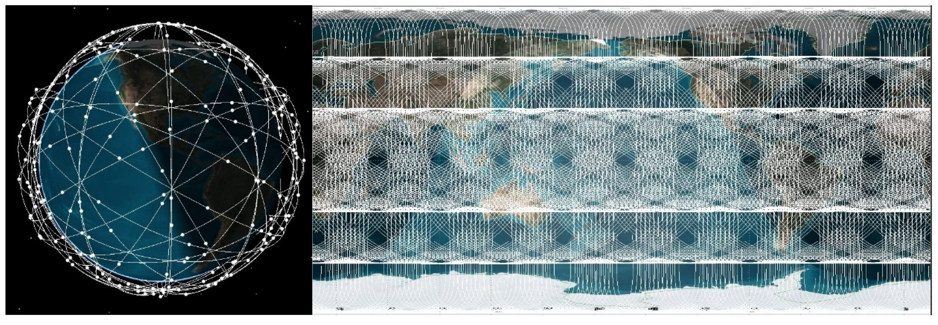
The experiment involved designing a LEO satellite constellation. It is designed to have three unique orbital altitudes, three dissimilar orbital inclinations, enabling it to achieve worldwide coverage. The constellation parameters are shown in Table 1. The simulation results of the satellite constellation are presented in Figure 1. The experiment selects the L-band with the aim of evaluating the Doppler positioning performance of low Earth orbit satellites in the L-band, in order to provide a basis for LEO-enhanced GNSS or combined LEO and GNSS positioning.

Table 1.
Main parameters of designed constellations.
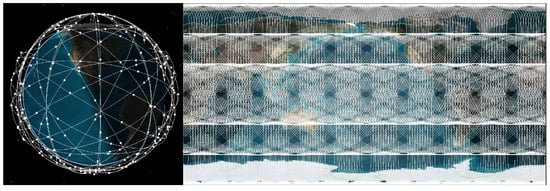
Figure 1.
3D and 2D views of the constellation.
The experiment selected five arbitrary locations at low, medium, and high latitudes, as shown in Table 2, as observation points. The elevation angle was set to 10°, and the observation duration was 12 h with a time interval of 1 min. The experiment analyzed the impact of different error magnitudes on Doppler positioning performance, including orbital errors and satellite velocity errors. The evaluation metrics chosen were the root mean square error (RMSE) and standard deviation of the positioning results in the X, Y, and Z directions, as well as the three-dimensional positioning results. RMSE was used to assess the difference between predicted and true values, representing the accuracy of the positioning results. The standard deviation indicates the degree of dispersion of the positioning errors. The Doppler positioning error simulation strategy is shown in Table 3.
Table 2.
Location of reference points.
Table 3.
Doppler localization error simulation strategy.
5. Results and Discussion
5.1. Number of Visible Satellites and DGDOP
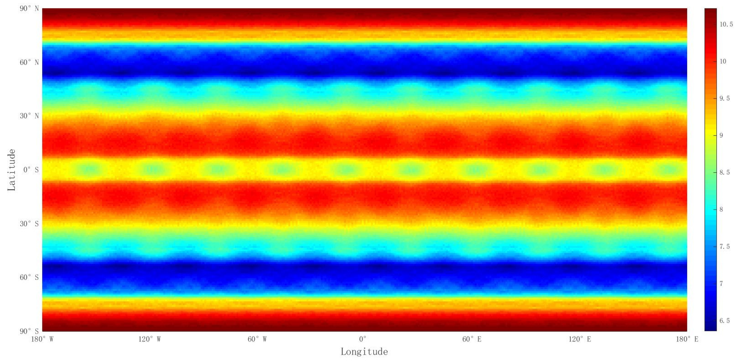
The experiment analyzed the variation of the global visible satellite count, with the results shown in Figure 2. The analysis revealed that, with an elevation angle of 10°, a maximum of about 10 satellites can be observed, while a minimum of 6 satellites can be observed. Within latitudes of 30° north and south, the visible satellite count ranges from 9 to 10. At latitudes of 60° north and south, the visible satellite count is around 6, while in the polar regions, the visible satellite count exceeds 10. Therefore, the constellation meets the positioning condition for instantaneous positioning, requiring the observation of at least four satellites.
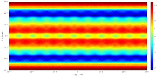
Figure 2.
Global average satellite visibility.
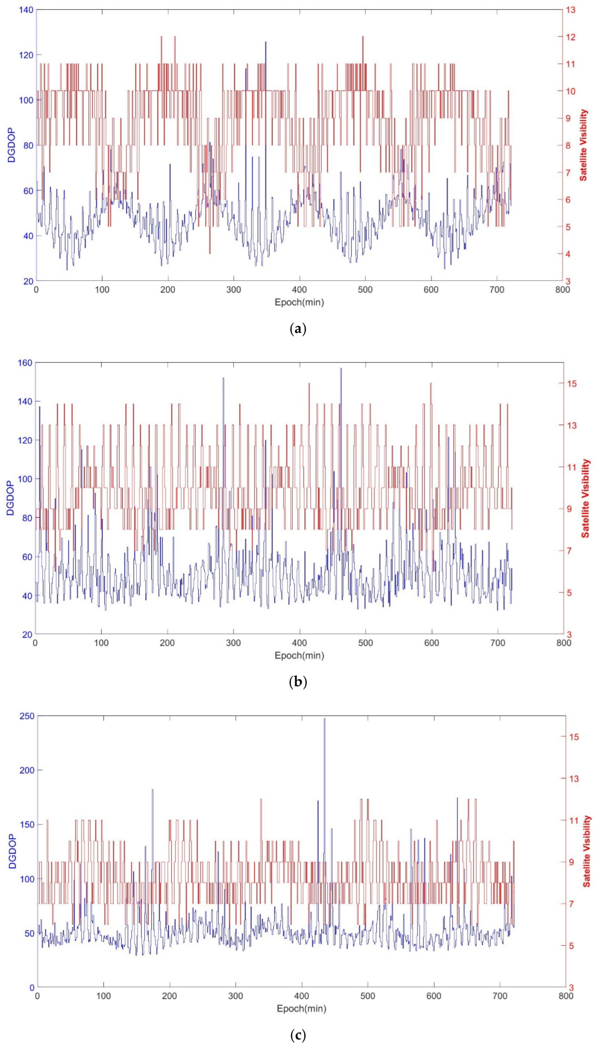
The experiment analyzed the average satellite visibility and average DGDOP values at five different locations, with the specific results shown in Figure 3 and Table 4. The average DGDOP value at Location 1 was 48.16, with a standard deviation of 10.91, and the average satellite visibility was 8.8; at Location 2, the average DGDOP value was 52.00, with a standard deviation of 14.78, and the average satellite visibility was 9.8; at Location 3, the average DGDOP value was 52.60, with a standard deviation of 18.84, and the average satellite visibility was 8.2; at Location 4, the average DGDOP value was 41.47, with a standard deviation of 18.3, and the average satellite visibility was 6.8; at Location 5, the average DGDOP value was 40.26, with a standard deviation of 12.46, and the average satellite visibility was 9.9. Through the analysis, it was found that DGDOP can be influenced by individual low-quality satellites, leading to the phenomenon where DGDOP increases as the number of visible satellites increases. From the overall data trend, it was observed that satellite visibility and DGDOP are negatively correlated, meaning that as the number of visible satellites decreases, DGDOP increases, and vice versa.
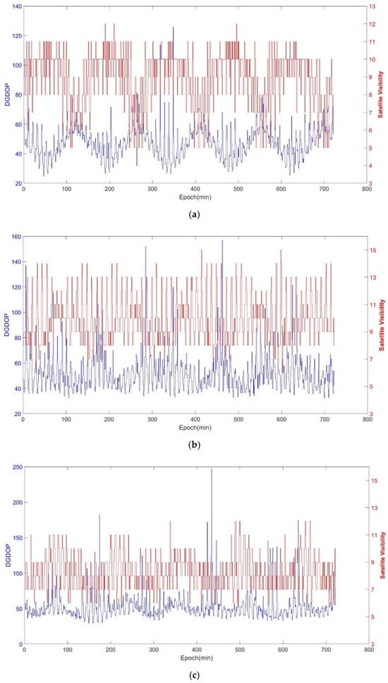
Figure 3.
Satellite visibility and DGDOP at 5 different locations. (a) Satellite visibility and DGDOP at Location 1; (b) satellite visibility and DGDOP at Location 2; (c) satellite visibility and DGDOP at Location 3; (d) satellite visibility and DGDOP at Location 4; (e) satellite visibility and DGDOP at Location 5.
Table 4.
DGDOP and average satellite visibility at different reference points.
5.2. The Impact of Satellite Orbit Errors on Positioning
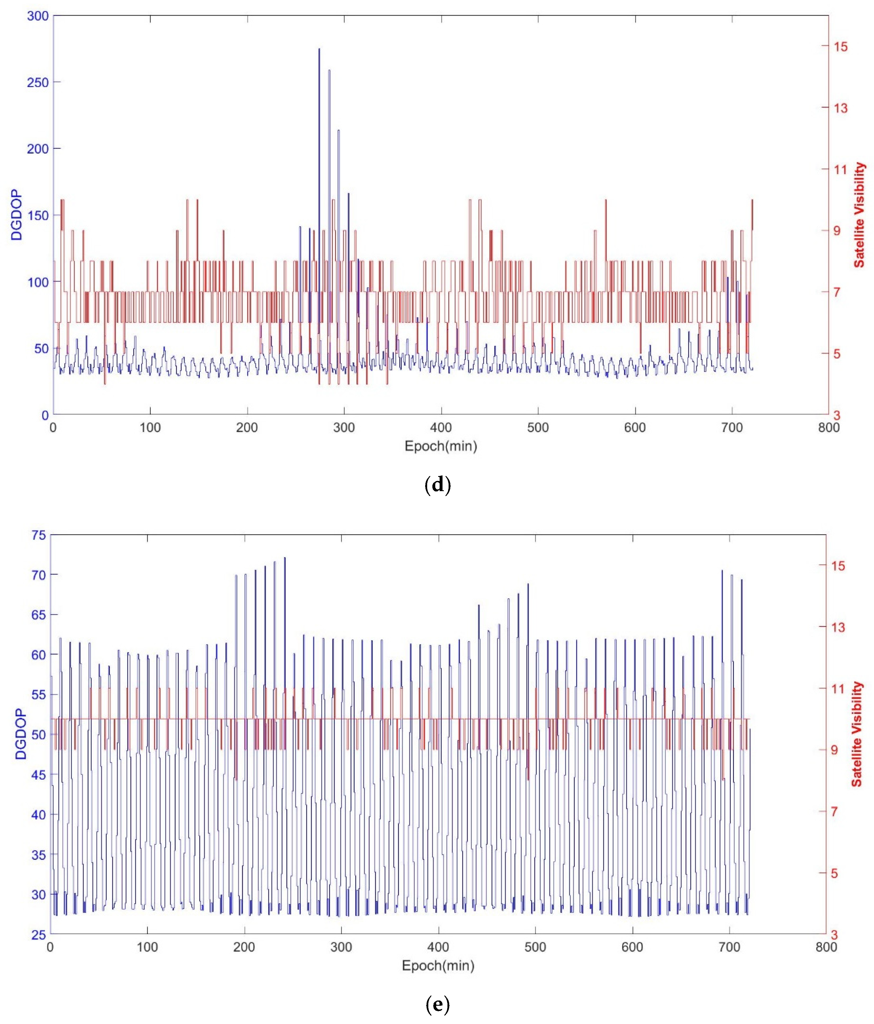
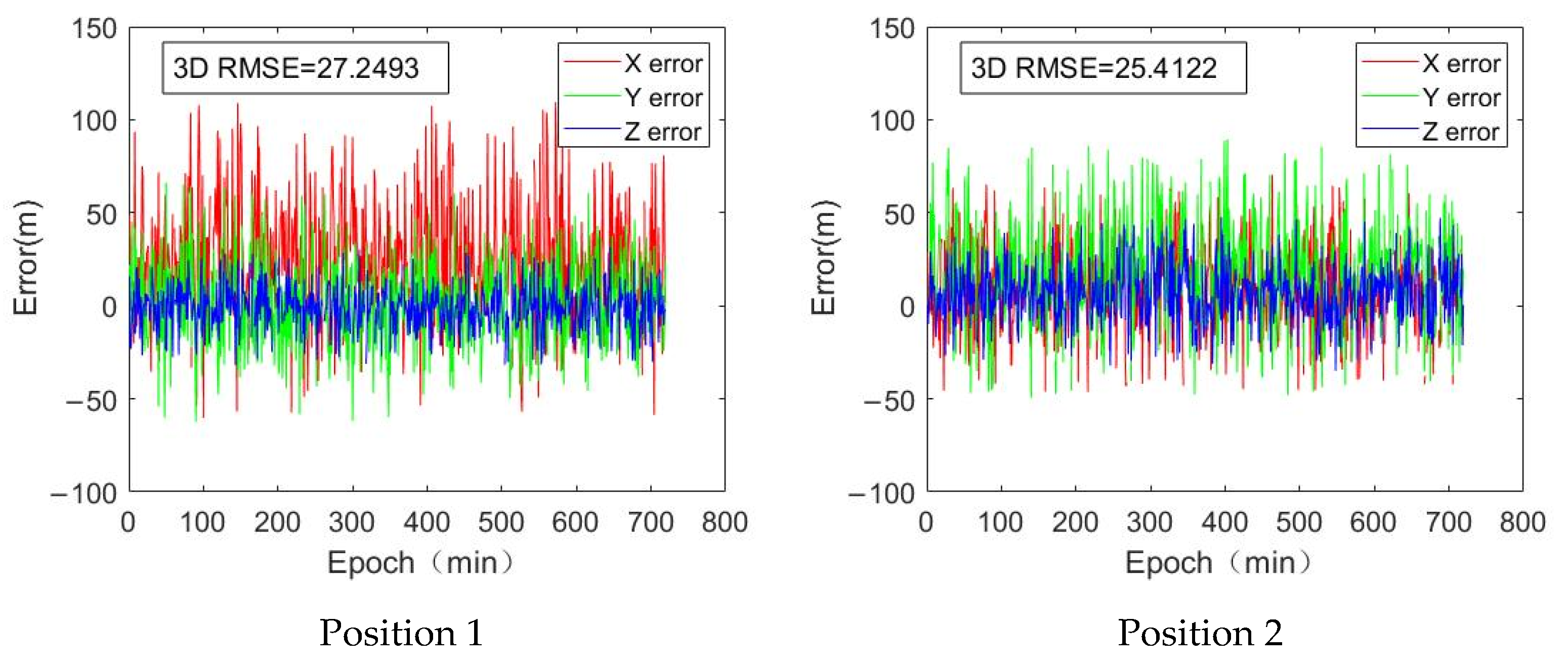
To analyze the impact of satellite orbital errors and satellite velocity errors on positioning results, the reference data with an elevation angle greater than 10°, zero orbital error, and zero satellite velocity error were first analyzed, with the specific results shown in Figure 4. The analysis revealed that in high-latitude regions, the 3D RMSE is lower, indicating better positioning accuracy. In mid- to low-latitude regions, the greater number of visible satellites there are, the better the positioning results.
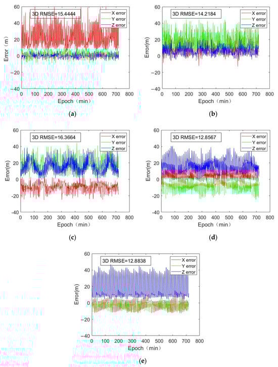
Figure 4.
Positioning results with no orbital error and no velocity error. (a) Position 1; (b) Position 2; (c) Position 3; (d) Position 4; (e) Position 5.
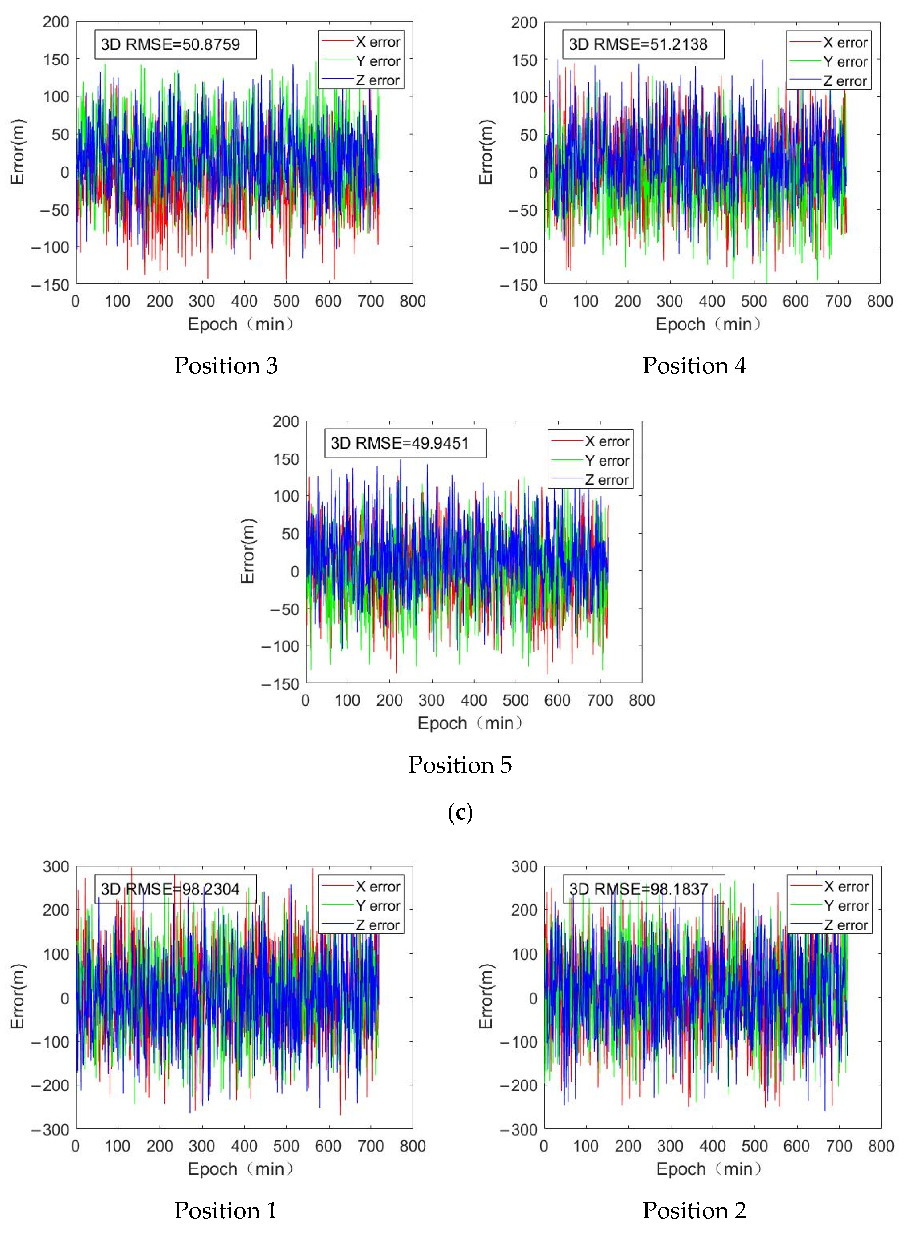
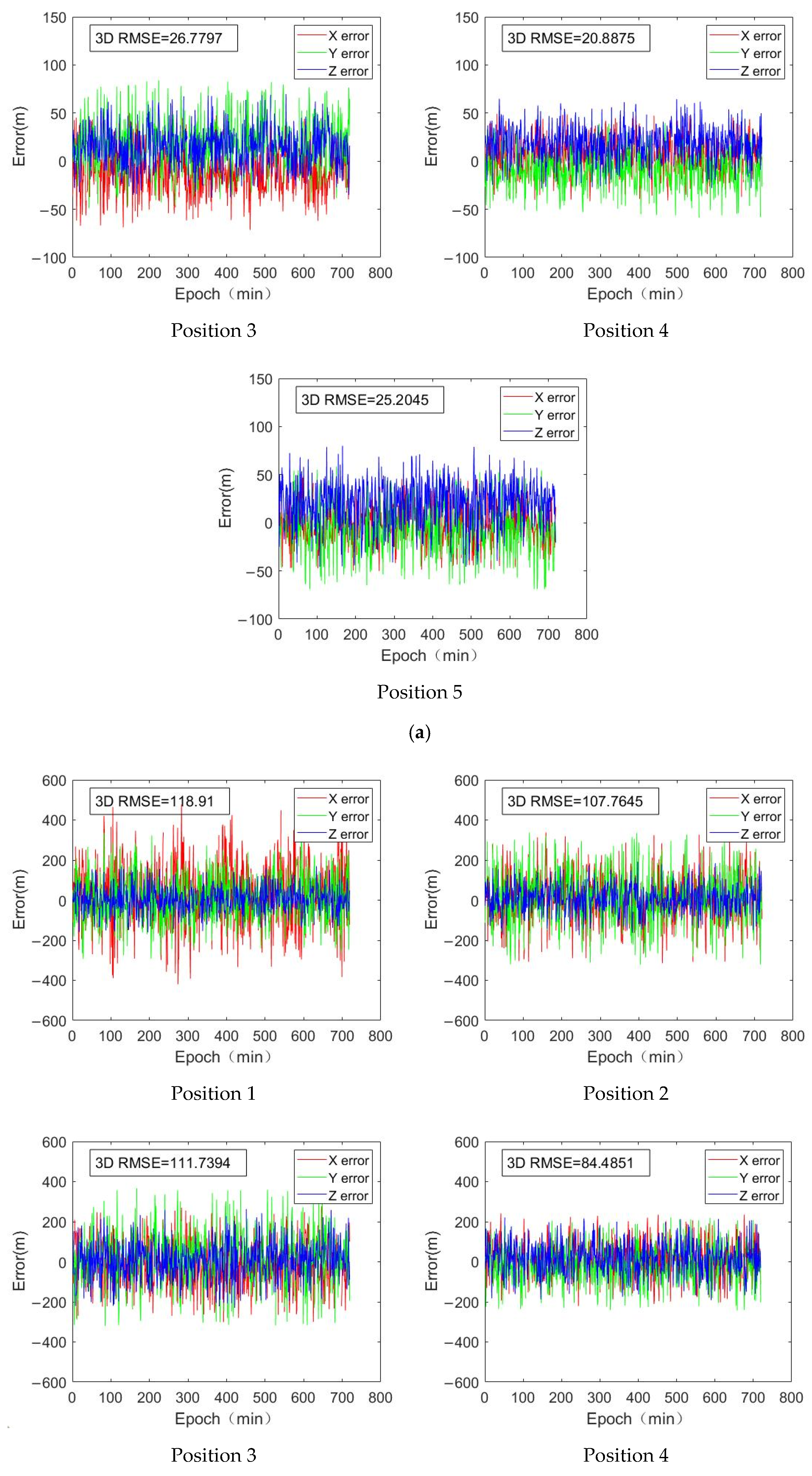
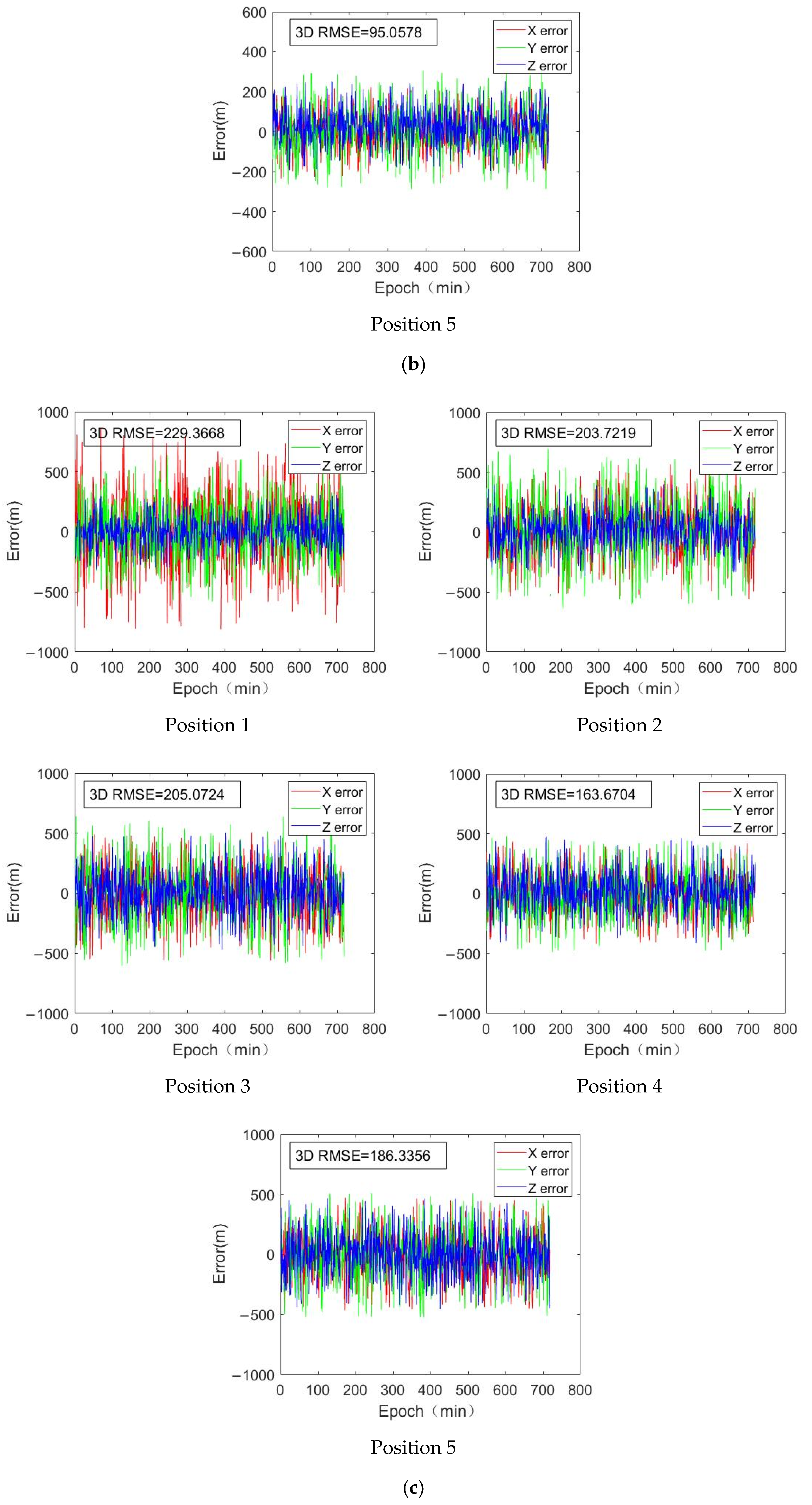
To analyze the impact of orbital errors on positioning results, orbital errors with a mean of 0 and standard deviations of 5 m, 10 m, 50 m, and 100 m, following a normal distribution, were introduced for each satellite during the solution process. In the positioning process, the effects of satellite clock drift, ionospheric error rates, tropospheric error rates, and Earth rotation effects on the errors were also considered. The specific results are shown in Figure 5. The analysis revealed that when the orbital error is within the 10 m range, the 3D RMSE error does not change significantly compared to the reference data with zero orbital error, and the errors remain within 20 m. However, when the orbital errors are 50 m and 100 m, the 3D RMSE errors are approximately 50 m and 100 m, respectively. Additionally, the position of the satellite does not have a significant effect on the positioning results. From this, it can be concluded that when the orbital error is small, its impact on the positioning results is not significant. As the orbital error increases, it becomes the dominant source of error. Therefore, one way to improve positioning accuracy is to control the orbital error of LEO satellites within a 10 m range, which can provide better observational precision.
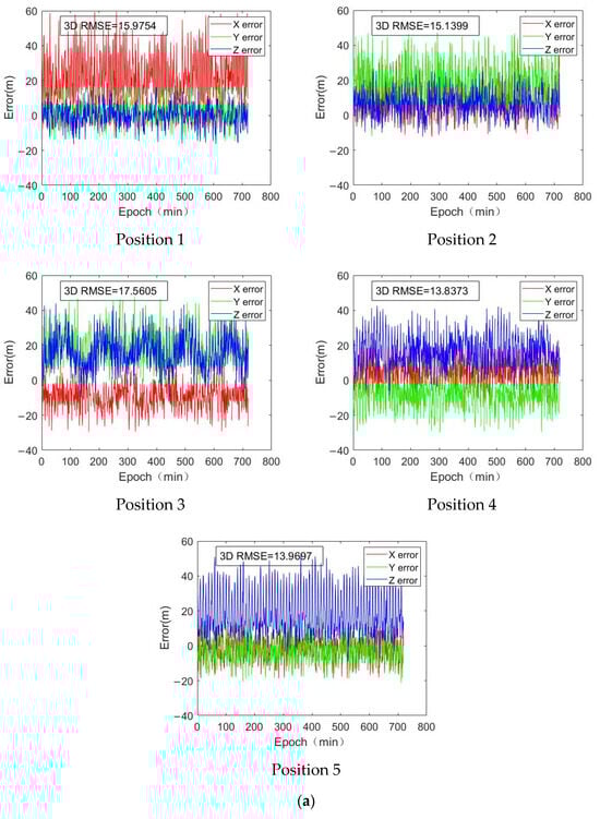
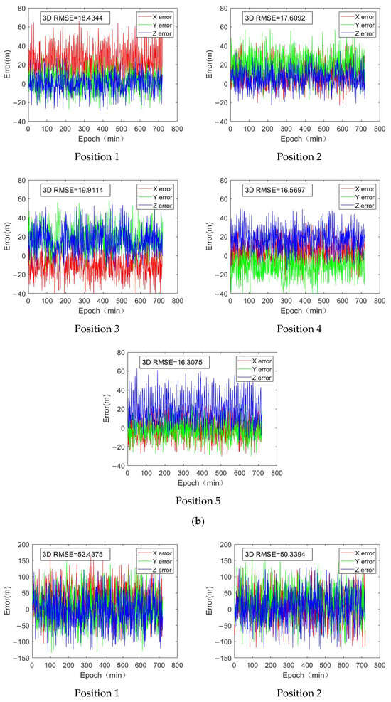

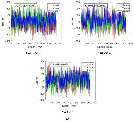
Figure 5.
Positioning results with orbital errors of different magnitudes. (a) The satellite orbital error is 5 m; (b) the satellite orbital error is 10 m; (c) the satellite orbital error is 50 m; (d) the satellite orbital error is 100 m.
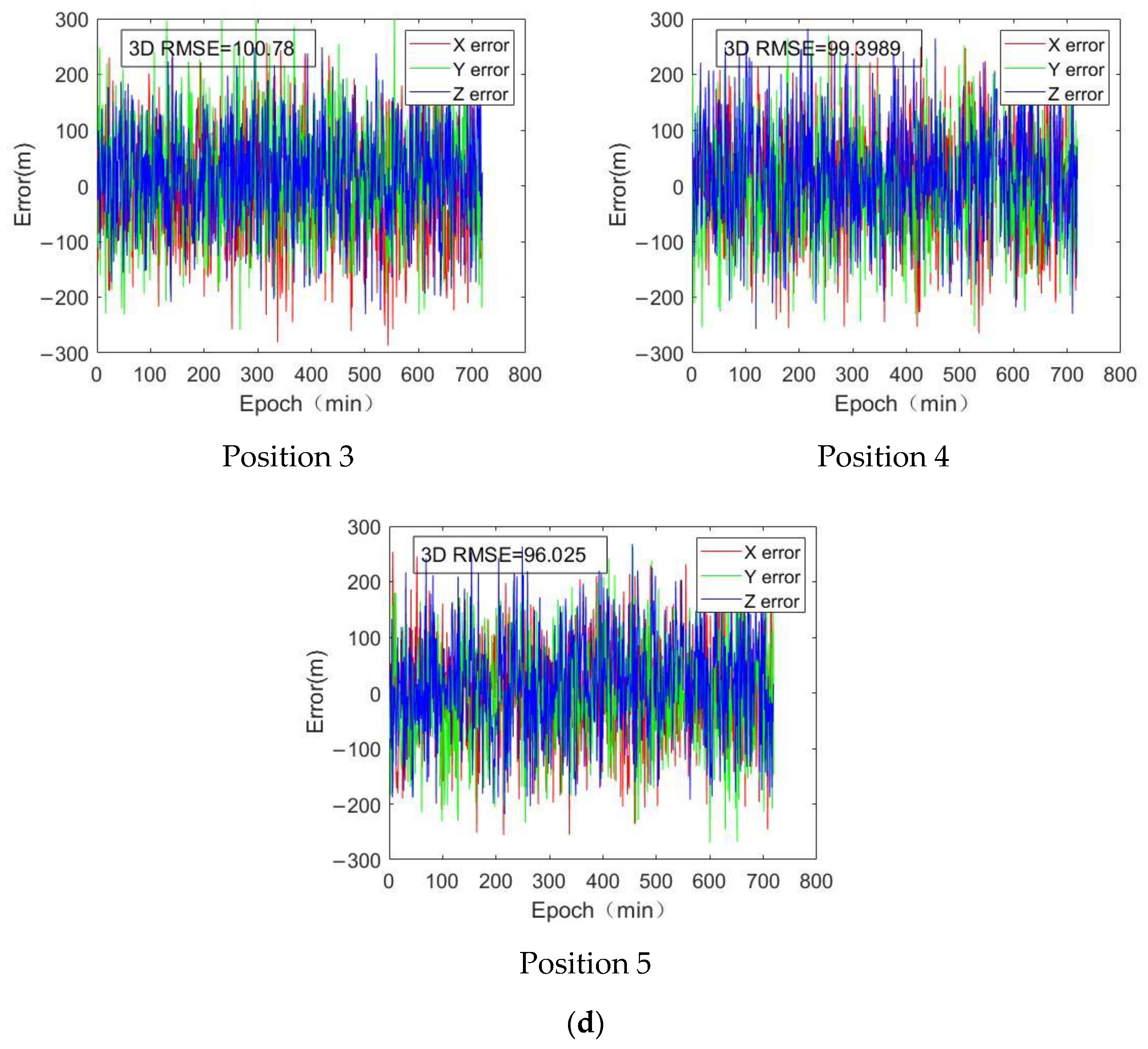
5.3. The Impact of Satellite Velocity on Positioning
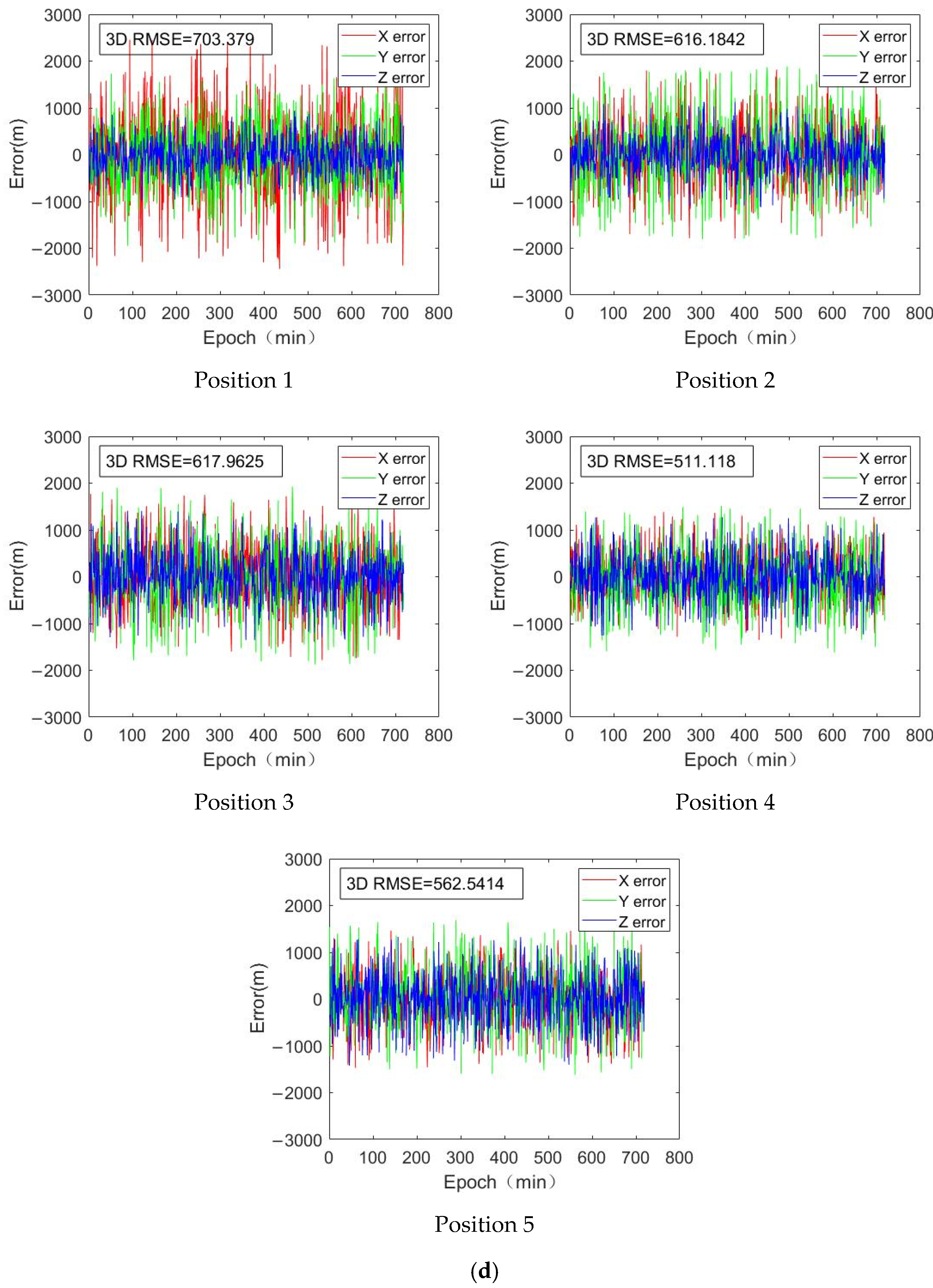
To analyze the impact of satellite velocity on positioning results, velocity errors with a mean of 0 and standard deviations of 0.1 m/s, 0.5 m/s, 1 m/s, and 3 m/s, following a normal distribution, were introduced for each satellite during the solution process. In the positioning process, the effects of satellite clock drift, ionospheric error rates, tropospheric error rates, and Earth rotation effects on the errors were also considered. The specific results are shown in Figure 6. The analysis found that satellite velocity errors have a significant impact on positioning results. When the satellite velocity error is within 0.5 m/s, the 3D RMSE error is within 100 m. However, when the satellite velocity error increases to 1 m/s and 3 m/s, the 3D error increases to approximately 200 m and 600 m, respectively. In high-latitude regions, the positioning accuracy is slightly better than in mid- and low-latitude regions. It can be observed that when the satellite velocity error is less than 0.1 m/s, the impact on the positioning result is negligible. As the satellite velocity increases, the impact on positioning results becomes more severe. Therefore, one way to improve positioning accuracy is to control the satellite velocity error of LEO satellites within a range of 0.1 m/s.
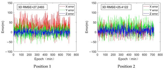
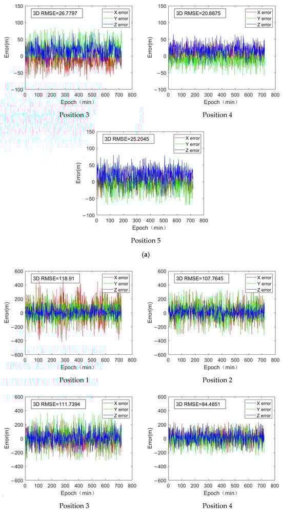

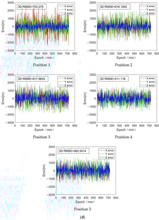
Figure 6.
Positioning results with satellite velocity errors of different magnitudes. (a) The satellite velocity error is 0.1 m/s; (b) the satellite velocity error is 0.5 m/s; (c) the satellite velocity error is 1 m/s; (d) the satellite velocity error is 3 m/s.
5.4. Normal Positioning Error
Based on the above analysis, to achieve a Doppler instantaneous positioning error within 50 m and meet the daily positioning requirements, the LEO satellite orbit error should be controlled within 10 m, and the LEO satellite velocity error should be controlled within 0.1 m/s. The positioning results are shown in Table 5. From the table, it can be observed that the positioning error in the X-direction is approximately between 20 and 41 m, with a standard deviation ranging from 20 to 34 m. The positioning error in the Y-direction is between 23 and 35 m, with a standard deviation ranging from 24 to 30 m. The positioning error in the Z-direction is between 15 and 31 m, with a standard deviation ranging from 16 to 26 m. The 3D RMSE indicates a positioning accuracy of within 30 m.
Table 5.
Positioning results for different reference points.
6. Conclusions
This paper derives the mathematical principles of Doppler-based instantaneous positioning and DGDOP, and provides models for satellite clock drift rate, ionospheric delay rate, tropospheric delay rate, and Earth rotation effect error rate. It then analyzes the relationship between the number of visible satellites and DGDOP, revealing a negative correlation between the two. Based on this, the effects of orbital errors and satellite velocity errors at different magnitudes on positioning performance are compared. It is verified that under normal atmospheric conditions with an orbital error of 10 m and a satellite velocity error of 0.1 m/s, positioning accuracy of within 30 m can be achieved. With the continuous development of LEO satellites, which can provide a large number of opportunity signals, positioning capabilities will continue to improve, demonstrating that Doppler-based positioning with LEO satellites can serve as a backup to GNSS.
Author Contributions
Methodology, M.C. and W.L. (Wanli Li); Software, Y.S.; Formal analysis, X.S.; Investigation, Y.L. and J.Y.; Data curation, W.L. (Wei Lv); Writing—original draft, X.L.; Supervision, W.Z. All authors have read and agreed to the published version of the manuscript.
Funding
This research was funded by [School Education and Teaching Research Project] grant number [JXYJ2024032].
Data Availability Statement
The original contributions presented in this study are included in the article. Further inquiries can be directed to the corresponding author.
Conflicts of Interest
The authors declare no conflict of interest.
References
- Liu, Z.; Xia, F.; Xu, C. Modeling and Simulation of GNSS Navigation Messages Based on MWORKS. Softw. Guide 2023, 10, 11–18+253. [Google Scholar]
- Ge, Y.; Xue, L.; Li, J. Analysis of the development trends of US Army PNT capabilities. Navig. Position. Timing 2019, 6, 12–18. [Google Scholar]
- Liu, H.; Fang, S.; Fan, Y.; Ma, S. Review of navigation via signals of opportunity. J. Ordnance Equip. Eng. 2022, 7, 78–86+158. [Google Scholar]
- Li, M.; Huang, T.; Li, W.; Zhao, Q. Overview of Low Earth Orbit (LEO) Navigation Augmentation Technology. J. Geomat. 2024, 49. [Google Scholar] [CrossRef]
- Guo, F.; Yang, Y.; Ma, F.; Zhu, Y.; Liu, H.; Zhang, X. Instantaneous velocity determination and positioning using Doppler shift from a LEO constellation. Satell. Navig. 2023, 4, 9. [Google Scholar] [CrossRef]
- Liu, Z.; Zhang, Y.; Zhang, X.; Cheng, Y. Research and Simulation of Single Star Positioning Algorithm Based on Low Earth Orbit Satellite. In Proceedings of the China Satellite Navigation Academic Annual Conference, Harbin, China, 23–25 May 2018. [Google Scholar]
- Deng, Z.; Gao, H.; Wang, L. Mutiple-scene Doppler Locating Method forLEO Satellite Navigation System. Radio Eng. 2017, 47, 49–53. [Google Scholar]
- Qin, H.; Zhang, Y.; Shi, G.; Wang, D. Doppler positioning technology based on Globalstar signals of opportunity. J. Beijing Univ. Aeronaut. Astronaut. 2023, 1–10. [Google Scholar] [CrossRef]
- Qin, H.; Tan, Z.; Cong, L.; Zhao, C. Positioning technology based on IRIDIUM signals of opportunity. J. Beijing Univ. Aeronaut. Astronaut. 2019, 9, 1691–1699. [Google Scholar] [CrossRef]
- Qin, H.; Tan, Z.; Cong, L.; Zhao, C. Positioning technology based on ORBCOMM signals of opportunity. J. Beijing Univ. Aeronaut. Astronaut. 2020, 11, 1999–2006. [Google Scholar] [CrossRef]
- Qin, H.; Zhang, Y. Positioning technology based on starlink signal of opportunity. J. Navig. Position. 2023, 1, 67–73. [Google Scholar] [CrossRef]
- Liang, J. Investigation on Iridium STL Positioning Method. Doctoral Dissertation, Huazhong University of Science and Technology, Wuhan, China, 2018. [Google Scholar]
- Fan, H. Effect of Low Earth Orbit Enhancement Constellation on GNSS Precise Point Positioning. Doctoral Dissertation, Taiyuan University of Technology, Taiyuan, China, 2023. [Google Scholar]
- Jiang, X.; Chen, X.; Ma, M.; Wang, Y.; Liang, R.; Yang, Z. Comparative Evaluation of Navigation Enhancement Performanceof Typical LEO Satellite Systems; GNSS World of China: Beijing, China, 2021. [Google Scholar]
- Xu, G.; Xu, Y. GPS Theory, Algorithms and Applications; Tsinghua University Press: Beijing, China, 2017. [Google Scholar]
- Khairallah, N.; Kassas, Z.M. Ephemeris closed-loop tracking of LEO satellites with pseudorange and Doppler measurements. In Proceedings of the 34th international technical meeting of the satellite division of the Institute of Navigation (ION GNSS+ 2021), St. Louis, MO, USA, 20–24 September 2021; pp. 2544–2555. [Google Scholar]
- Zhou, Q. Beidou Navigation Enhancement Simulation Research Based on LEO Constellation. Doctoral Dissertation, Shandong University of Technology, Zibo, China, 2022. [Google Scholar]
- Hein, G.W. Status, perspectives and trends of satellite navigation. Satell. Navig. 2020, 1, 1–12. [Google Scholar] [CrossRef] [PubMed]
- Xie, X. Analysis and discussion on the use of NBCORS system RTK technology for real estate surveying. Zhejiang Land Resour. 2015, 7, 2. [Google Scholar]
- Zhang, Y.; Li, Z.; Shi, C.; Jing, G. Doppler Positioning Performance of LEO Mega Constellation. Space-Integr.-Ground Inf. Netw. 2024, 5, 84–94. [Google Scholar]
- Bao, R.; Tang, C.; Hu, X.; Zhou, S.; Cao, Y.; Yang, Y. Study on the Accuracy Evaluation of BeiDou Broadcast Ionospheric Model. J. Beijing Univ. Aeronaut. Astronaut. 2023. [Google Scholar] [CrossRef]
- Nava, B.; Coisson, P.; Radicella, S.M. A new version of the nequick ionosphere electron density model. J. Atmos. Sol.-Terr. Phys. 2008, 70, 1856–1862. [Google Scholar] [CrossRef]
- Yu, X. The Key Technology Research on the High Precise Monitoring Management for Vehicle safety Operation Based on GNSS. Doctoral Dissertation, China University of Mining and Technology, Xuzhou, China, 2017. [Google Scholar]


Disclaimer/Publisher’s Note: The statements, opinions and data contained in all publications are solely those of the individual author(s) and contributor(s) and not of MDPI and/or the editor(s). MDPI and/or the editor(s) disclaim responsibility for any injury to people or property resulting from any ideas, methods, instructions or products referred to in the content. |
© 2025 by the authors. Licensee MDPI, Basel, Switzerland. This article is an open access article distributed under the terms and conditions of the Creative Commons Attribution (CC BY) license (https://creativecommons.org/licenses/by/4.0/).