Abstract
Evapotranspiration (ET) plays a crucial role in the surface water cycle and energy balance, and accurate ET estimation is essential for study in various domains, including agricultural irrigation, drought monitoring, and water resource management. Remote sensing (RS) technology presents an efficient approach for estimating ET at regional scales; however, existing RS retrieval algorithms for ET are intricate and necessitate a multitude of parameters. The land surface temperature–vegetation index (LST-VI) space method and statistical regression by machine learning (ML) offer the benefits of simplicity and straightforward implementation. This study endeavors to identify the optimal long-term sequence LST-VI space method and ML for ET estimation under conditions of limited observed variables, (LST, VI, and near-surface air temperature). A comparative analysis of their performance is undertaken using ground-based flux observations and MOD16 ET data. The findings can be summarized as follows: (1) Long-term remote sensing data can furnish a more comprehensive background field for the LST-VI space, achieving superior fitting accuracy for wet and dry edges, thereby enabling precise ET estimation with the following metrics: correlation coefficient (r) = 0.68, root mean square error (RMSE) = 0.76 mm/d, mean absolute error (MAE) = 0.49 mm/d, and mean bias error (MBE) = −0.14 mm. (2) ML generally produces more accurate ET estimates, with the Random Forest Regressor (RFR) demonstrating the highest accuracy: r = 0.79, RMSE = 0.61 mm/d, MAE = 0.42 mm/d, and MBE = −0.02 mm. (3) Both ET estimates derived from the LST-VI space and ML exhibit spatial distribution characteristics comparable to those of MOD16 ET data, further attesting to the efficacy of these two algorithms. Nevertheless, when compared to MOD16 data, both approaches exhibit varying degrees of underestimation. The results of this study can contribute to water resource management and offer a fresh perspective on remote sensing estimation methods for ET.
1. Introduction
Evapotranspiration (ET) denotes the process by which water is transferred from surface soil or vegetation into the atmosphere. It is estimated that approximately 60–70% of precipitation ultimately returns to the atmosphere through evapotranspiration, and this process consumes roughly 50% of the available radiant energy at the surface, commonly referred to as latent heat flux (LE) [1,2,3]. T Consequently, evapotranspiration constitutes a vital component of the surface water and energy balances, exerting a significant influence on the distribution of precipitation and radiant energy. Accurate and efficient monitoring of evapotranspiration is imperative for gaining insights into surface hydrological processes and the dynamics of the surface water cycle [4]. Moreover, evapotranspiration serves as a crucial indicator of vegetation water demand and is essential for drought monitoring. By comprehending the spatiotemporal distribution characteristics of evapotranspiration, drought early warning can be effectively implemented, and the supply and demand of surface water can be quantified. This holds immense significance for enhancing water resource management, optimizing farmland irrigation practices, and improving water use efficiency [5]. Direct observation of evapotranspiration is often challenging, and methods such as eddy covariance technology, lysimeters, scintillometers, and Bowen ratio energy balance observation systems are primarily employed for in situ observations of evapotranspiration [6,7]. Although these methods offer good accuracy and are well-established, they are limited to point-scale observations, which are spatially discontinuous and unable to capture regional-scale spatial variability. Furthermore, their high costs make them impractical for large-area studies [8]. Remote sensing technology, with its advantages of extensive observation coverage and high efficiency, provides a means for monitoring evapotranspiration that is both spatially and temporally continuous and cost-effective.
In recent years, retrieval algorithms for evapotranspiration utilizing remote sensing observations have undergone continuous development. These algorithms predominantly encompass the one-source energy balance model, the two-source energy balance model, the Penman–Monteith model, the feature space method, and empirical regression methods. These methodologies have found widespread application, each one possessing its unique advantages and limitations [9,10,11,12,13,14,15]. The energy balance model, in particular, estimates evapotranspiration by first calculating the components of net radiation flux, namely sensible heat flux and soil heat flux, and subsequently determining the latent heat flux utilized for water evaporation. The one-source energy balance model treats the surface as uniform vegetation without distinguishing it from bare soil, such as in the SEBAL [14], SSEB [16], METRIC [17], and SEBS models [18], whereas the two-source energy balance model distinguishes between surface vegetation and bare soil, calculating resistances separately to estimate evapotranspiration, such as in the ALEXI [19] and TSEB models [20]. The Penman–Monteith model estimates evapotranspiration based on the Penman–Monteith equation, such as in the MOD16 model [21]. These models are all grounded in solid theoretical foundations, and in recent years, numerous studies have applied these algorithms and compared their accuracy differences [22,23,24,25,26]. However, no consensus has been reached on which model is superior, emphasizing the need to consider specific environmental characteristics when choosing an appropriate model for estimating ET [27]. The selection process must take into account factors such as land cover types, climate conditions, data availability, and the inherent limitations of each model. It should be noted that energy balance models have complex calculation processes, require numerous parameters, and are computationally inefficient. The Penman–Monteith model also requires many meteorological parameters, limiting its applicability in regions with sparse observational data.
The feature space method leverages the triangular or trapezoidal feature space, constructed by surface temperature and vegetation cover, to delineate the wet and dry limits (the upper and lower confines of the feature space) of the target region. This approach facilitates the estimation of evapotranspiration and the differentiation between vegetation transpiration and soil evaporation, while circumventing the uncertainties inherent in the intricate calculations of aerodynamic and surface resistances [28]. Owing to its simplicity and efficiency, the feature space method has gained widespread development and application, and its accuracy has been well established [12,29,30]. Essentially, the feature space constitutes a triangular or trapezoidal area enclosed by surface temperature and vegetation cover or the vegetation index within a two-dimensional coordinate system. The upper and lower boundaries of this feature space, known as the wet and dry edges, can be determined through fitting or theoretical derivation [28]. These edges represent the maximum and minimum surface temperatures at a specific vegetation cover or index, corresponding to conditions of extreme dryness and complete saturation, respectively. Subsequently, the water and thermal status of the target pixel can be determined based on its relative position in the feature space [28], effectively circumventing the challenge of accurately calculating surface impedance under partial vegetation cover, thereby demonstrating significant advantages [29,31]. In addition, Tang et al. [32,33] further proposed the concept of a critical edge based on the wet edge and dry edge to distinguish between the effects of soil surface moisture and root zone moisture, and this concept has been widely applied [34,35]. This two-dimensional feature space is widely used in studies such as soil moisture estimation and evapotranspiration retrieval [36,37]. However, whether the feature space can accurately describe the extreme temperatures of a target area under certain atmospheric forcing conditions largely depends on the appropriateness of the target area (i.e., the background field) size, which introduces uncertainties into the feature space [38]. Some studies have utilized the difference between air temperature and land surface temperature in place of land surface temperature to construct feature spaces, thereby reducing to some extent the impact of spatial variations in air temperature within the study area on the results [39,40]. Cheng et al. [41] proposed the construction of a three-dimensional feature space comprising land surface temperature–vegetation index–air temperature, as an alternative to the traditional two-dimensional feature space, to mitigate the influence of differences in atmospheric forcing conditions. Additionally, some scholars have suggested using long-term remote sensing observation data to determine feature spaces and wet/dry edges, specifically by employing multitemporal observation data at the pixel scale to define feature spaces and wet/dry limits, enabling the feature spaces to encompass a more comprehensive range of soil water and thermal conditions [42,43,44,45]. However, studies have shown that due to differences in atmospheric forcing conditions over time, the correlation between surface temperature and surface moisture conditions based on long-term remote sensing observations is unstable, introducing errors into the derivation of surface evapotranspiration and soil moisture [28,46]. Nevertheless, long-term data provide new insights for determining the wet and dry edges, and there is still potential to improve the feature space by constructing a more accurate feature space through a combination of spatial and temporal domains [41].
The statistical regression method directly fits the empirical relationship between remote sensing information and ground-observed evapotranspiration. This method is simple to compute and, with the maturity of machine learning algorithms and big data processing, the accuracy of estimating evapotranspiration using statistical regression methods has gradually improved. For example, Carter et al. [47] compared the accuracy of estimating evapotranspiration using 10 machine learning algorithms combined with remote sensing data and found that the bootstrap aggregation (bagging) regression tree had the best accuracy (validation RMSE = 19.91 W/m2); Cheng et al. [48] compared estimations of evapotranspiration in the Haihe River Basin, China, using different types of input variables (vegetation growth, surface humidity, radiant energy, and other related variables) combined with machine learning algorithms. The results showed that more input variables led to a higher accuracy, with vegetation growth contributing the most to ET estimation. Previous studies using statistical regression methods to estimate ET have achieved high accuracies, but they often require numerous input variables, increasing the computational burden. Currently, few studies have discussed whether comparable accuracy can be achieved with reduced input variables.
This study focuses on the Beijing region and its surroundings in China, analyzing and comparing the accuracy of estimating evapotranspiration (ET) using the Long-Term Sequence Feature Space Method (LTSFSM) and statistical regression methods based on machine learning. The main objectives include the following: (1) exploring the most appropriate spatiotemporal domain size and the accuracy of ET estimation using the LTSFSM with limited input variables; (2) comparing the ET estimation accuracy of different machine learning algorithms under limited input variables to determine the optimal algorithm; and (3) comparing the spatial distribution trends of ET estimated by different algorithms.
2. Study Area and Data Collection
2.1. Study Area
Beijing is located at the northwestern tip of the North China Plain, inland yet relatively near the Bohai Sea. Its geographical coordinates span from 115°24′E to 117°30′E longitude and from 39°28′N to 41°05′N latitude. The topography of Beijing slopes downwards from northwest to southeast, with mountains encircling it on three sides: the west, north, and northeast. To the west, the Western Mountains of the Taihang Mountain Range rise majestically, to the north lies the Jundu Mountain of the Yanshan Mountain Range, and to the southeast stretches the Beijing Plain, gently declining towards the Bohai Sea. Beijing boasts a variety of landforms, encompassing mountains, hills, alluvial fans, and piedmont plains. The mountainous regions mostly have an altitude ranging between 300 and 1500 m, while the plains generally lie at an altitude of 20 to 60 m. Beijing experiences a temperate monsoon climate characterized by distinct seasons and concurrent rainy and hot periods. Summers are marked by heat and rainfall, while winters are cold and dry. The annual mean temperature hovers between 10 and 12 °C, and the annual average precipitation exceeds 700 mm, with the bulk of the rainfall occurring in summer, particularly in July and August. Consequently, Beijing’s diverse topography and landforms give rise to considerable spatial variations in evaporation conditions. For this study, Beijing and its surrounding areas were selected as the research region, where atmospheric forcing conditions are relatively uniform, fulfilling the spatial domain requirements for estimating evapotranspiration using the feature space method.
2.2. Data Collection
2.2.1. Flux Observations
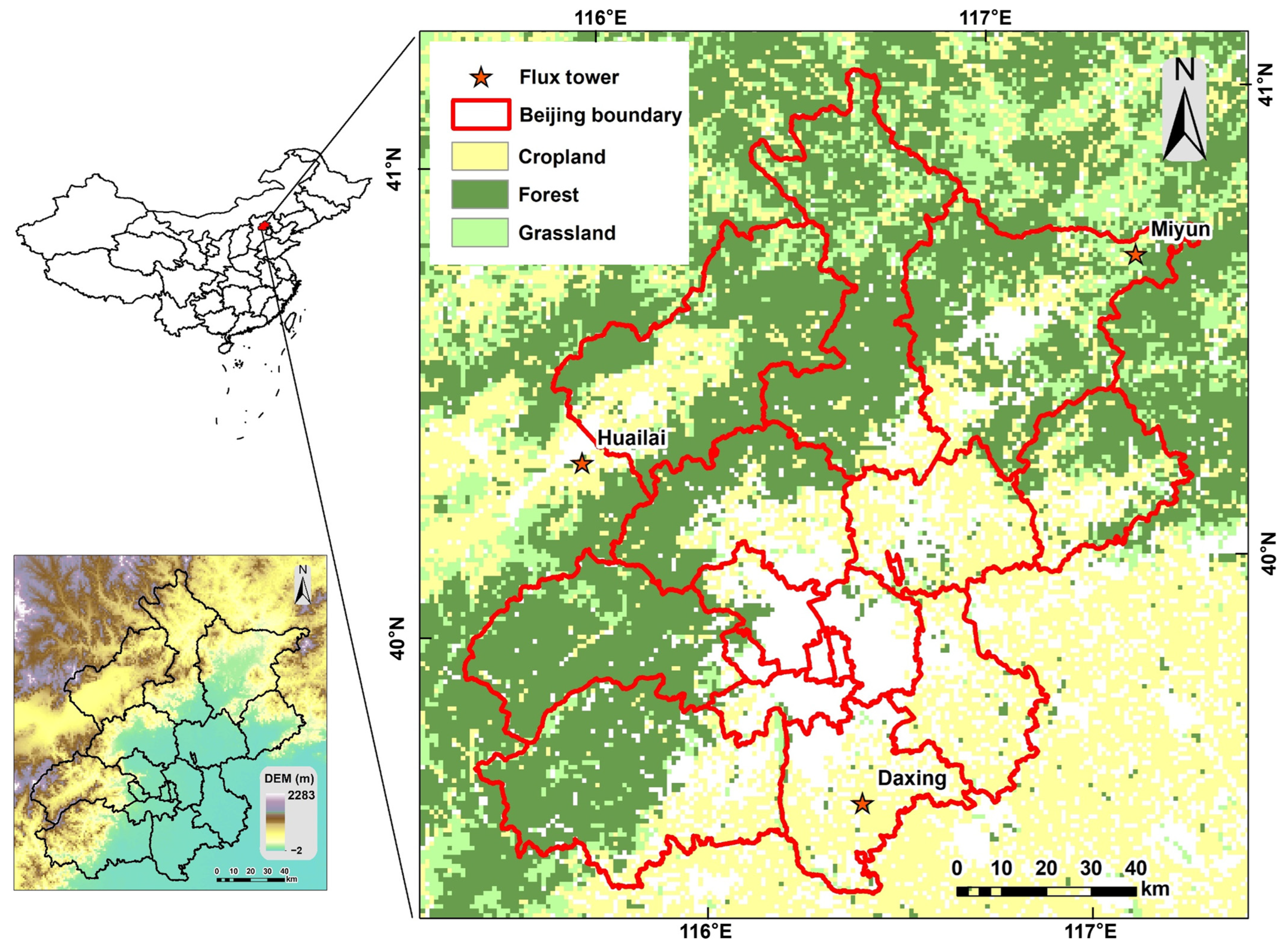
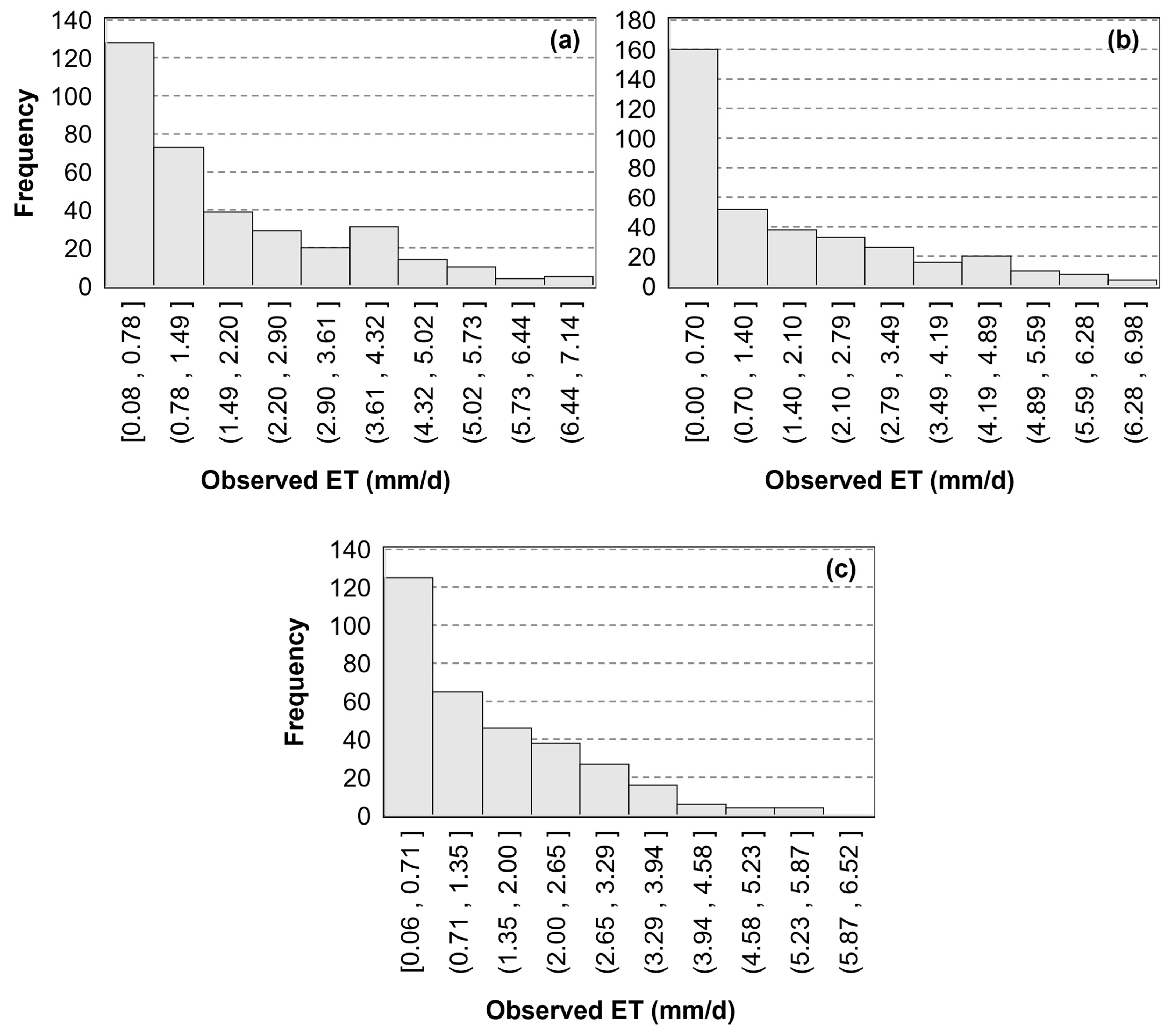
In this study, we utilized flux observation data (daily evapotranspiration) from three sites (Daxing, Huailai, and Miyun, obtained from ChinaFLUX (https://www.chinaflux.org/, accessed on 9 May 2022) for model development and validation (Table 1). The locations of these sites are shown in Figure 1. Daxing and Huailai were monitoring sites for agricultural ecosystems, primarily focusing on crop ecosystems with corn-wheat rotation. The observation periods for these sites were from 2008 to 2010 and 2016, respectively. Miyun was a monitoring site for forest ecosystems, with an observation period from 2008 to 2010. Due to the issue of energy imbalance in flux observations, we employed the Bowen ratio energy balance closure method to screen and correct the raw observed data, the details of which can be found in a study by Wang et al. [49]. Based on the geographical location of the flux towers and the observation period, the ET values from the corresponding pixel and date in the ET map simulated by the model were matched with the flux observations for validation. After screening and correction, a total of 1052 samples were available for this study, including 353 samples from the Daxing site, 332 samples from the Huailai site, and 367 samples from the Miyun site. The numerical distribution is shown in Figure 2. The observed mean daily evapotranspiration was 1.82 ± 1.63 mm/day at the Daxing site, 1.46 ± 1.26 mm/day at the Huailai site, and 1.64 ± 1.68 mm/day at the Miyun site.

Table 1.
Details of flux towers.

Figure 1.
Study area.

Figure 2.
Histogram of flux towers’ observed ET: (a) Daxing, (b) Huailai, and (c) Miyun.
2.2.2. Remote Sensing Data
In this study, the remote sensing data utilized for model input encompassed the Normalized Difference Vegetation Index (NDVI), land surface temperature (LST), daily average near-surface air temperature (NSATave), daily maximum near-surface air temperature (NSATmax), and daily minimum near-surface air temperature (NSATmin). The NDVI was calculated using MOD09 data at a daily resolution of 1 km (accessed at https://www.earthdata.nasa.gov/, accessed on 11 February 2025). The LST data were derived from a spatially and temporally continuous dataset of daytime surface temperatures generated by Zhang et al. [50,51,52] based on MODIS Terra satellite data, also at a daily scale and spatial resolution of 1 km (accessed from the Chinese National Qinghai–Tibet Plateau Scientific Data Center, (https://www.tpdc.ac.cn, accessed on 11 February 2025)). The near-surface air temperature data were sourced from the NSTADC (National Surface Air Temperature Daily Dataset for China), which was produced by Cheng et al. [53] using a combination of multivariate analysis and machine learning algorithms, providing daily average, maximum, and minimum near-surface air temperatures at a 1 km resolution (accessed at https://zenodo.org/records/10969448, accessed on 11 February 2025). The validity of these datasets has been demonstrated in their related studies [50,51,52,53].
Furthermore, we employed the MOD16 ET dataset, which is based on the Penman–Monteith model [54,55], to compare the simulation results of this study, allowing for an assessment of spatial distribution differences in ET under different algorithms.
3. Methodology
3.1. Long-Time-Series LST-VI Space Method
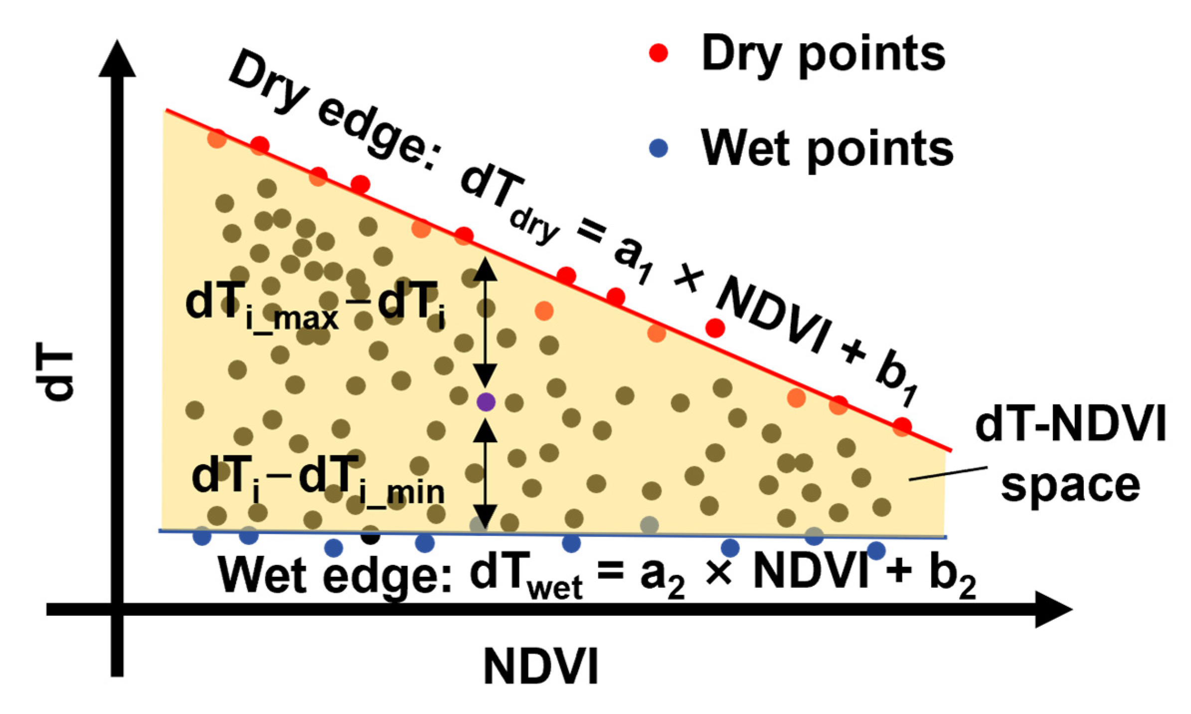
The feature space method determines the evaporation conditions of a target pixel based on its position in the feature space, as defined by its vegetation index and land surface temperature. In this study, the difference between land surface temperature and daily maximum near-surface air temperature (dT) was used as a substitute for land surface temperature to construct the feature space (Figure 3). The wet and dry edges of the feature space were fitted using dry pixels (red dots, Figure 3) and wet pixels (blue dots, Figure 3), respectively, according to the equation
where a1, b1, a2, and b2 are computed by linear fitting. Then, the evapotranspiration for the target pixel was calculated using the following equation:
where dTi_max, and dTi_min are the maximum and minimum dTs for the pixel i, which are determined by the dry and wet edges (Equations (1) and (2)). dTi is the dT of the pixel i. PET represents potential evapotranspiration, which was calculated using the Hargreaves–Samani (HS) model in this study due to its requirement for fewer parameters [56]:
where KT is the empirical coefficient, which is usually assumed to be 0.17, and Ra is the extraterrestrial radiation (MJ/m2). Traditional feature space methods are mostly based on a single-period image for calculation. However, the dT-NDVI feature space in this study attempted to compare the differences in feature spaces constructed from time series images of varying amounts.

Figure 3.
Sketch of dT-NDVI space. Note: the red lines indicate dry edges and blue lines indicate wet edges.
3.2. Machine Learning
In this study, a total of six machine learning algorithms were employed for fitting the correlation between input variables with the measured ET. The algorithms include the gradient boosting decision tree (GBDT), Random Forest Regression (RFR), partial least square regression (PLSR), K-Nearest Neighbors (KNN), backpropagation neural network (BPNN), and support vector regression (SVR). These machine learning algorithms have been widely applied in the field of remote sensing modeling, such as in soil moisture estimation [36,57], crop yield prediction [58,59], and vegetation leaf area index estimation [60,61], and they have proven to possess strong capabilities in nonlinear fitting and information mining. Therefore, this study attempted to analyze the accuracy of these algorithms in estimating ET when the input variables are limited.
(1) Gradient boosting decision tree (GBDT)
The core goal of the GBDT (gradient boosting decision tree) method is to train decision tree models using the gradient boosting strategy. The gradient boosting method updates model parameters based on the negative gradient direction of the loss function, iteratively adding new decision trees to minimize the loss function. In GBDT models, each decision tree attempts to correct the errors of the previous tree, thereby gradually improving the model’s predictive ability. The process is conducted as follows:
a. Estimate a constant value that minimizes the loss function as the initial model.
b. Calculate the negative gradient value of the loss function in the current model, which serves as an estimate of the residual.
c. Estimate the regions of the leaf nodes in the regression tree to fit the approximate values of the residuals.
d. Use linear search to estimate the values of the leaf node regions to minimize the loss function.
e. Update the decision tree.
f. Integrate the output results of all decision trees to obtain the final prediction.
(2) Random Forest Regression (RFR)
RFR is also an ensemble learning technique predominantly applied to regression problems. It leverages the power of multiple decision trees to enhance the precision and robustness of predictive outcomes. This is achieved by constructing a series of decision trees and then aggregating their predictions through averaging or majority voting. The Random Forest Regression algorithm encompasses the following key steps and characteristics:
a. Utilizing the bootstrap sampling technique, multiple sample sets are randomly drawn from the original training dataset, with each set maintaining the same size as the original.
b. For each of these sample sets, a decision tree is constructed. To foster diversity among the trees, randomness is introduced during the construction process. This includes, for instance, randomly selecting features for node splitting.
c. Each decision tree independently processes and predicts outcomes for new data points.
d. The final prediction is derived by averaging the results obtained from all individual decision trees, thereby harnessing the collective wisdom of the ensemble.
(3) Partial least square regression (PLSR)
Partial least squares (PLS) is a multivariate statistical method that combines Principal Component Analysis (PCA) with Ordinary Least Squares (OLS). It finds the optimal function match for a set of data by minimizing the sum of squared errors, and is used to analyze datasets containing multiple independent and dependent variables. The PLS method establishes a regression model by projecting the independent and dependent variables onto a new latent variable space. This new space maximizes the correlation between the latent variables of the independent and dependent variables, thereby effectively reducing the problem of multicollinearity and improving the predictive accuracy and interpretability of the model.
(4) K-Nearest Neighbors (KNN)
The KNN method fits the correlation by measuring the distance between different feature values. The term “K-Nearest Neighbors” refers to the concept that each sample can be represented by its k closest neighbors. The algorithm proceeds as follows:
a. Calculate the distance between the prediction data and each sample in the training dataset.
b. Sort these distances in ascending order.
c. Select the top k samples with the smallest distances as the “neighbors”.
d. Determine the categories of these k neighbors and their frequencies.
e. For classification problems, return the category with the highest frequency among the k neighbors as the prediction result. For regression problems, calculate the numerical average of the k neighbors and return it as the prediction result.
(5) Backpropagation neural network (BPNN)
The BPNN regression algorithm constitutes a multi-layer feedforward architecture that is trained utilizing the error backpropagation technique. This algorithm has found widespread application in diverse regression prediction scenarios. The principal stages of the BP neural network regression methodology are delineated as follows:
a. Network Initialization: The weights and biases connecting neurons across each layer are initialized in a random manner.
b. Forward Propagation of Input Signals: Input signals are propagated sequentially through the network, with the output of neurons at each layer being computed accordingly.
c. Error Calculation: The discrepancy between the network’s output and the desired output is quantified to determine the error.
d. Error Backpropagation: The error signal is propagated in reverse through the network, and adjustments are made to the weights and biases of neurons in each layer, guided by principles such as the gradient descent method or other pertinent optimization algorithms.
e. Iterative Training: The process encompassing steps (b) through (d) is iteratively executed until the preset maximum number of iterations is reached.
(6) Support vector regression (SVR)
The core goal of SVR is to map the input space and seek an optimal regression hyperplane in a high-dimensional space, such that as many data points as possible fall within the ε-tube surrounding the hyperplane, thereby achieving the goal of predicting continuous values. This hyperplane is positioned as close as possible to the data points and makes predictions within an allowable error range. The principal stages are as follows:
a. Data preprocessing, including feature selection, data normalization, etc.
b. Selecting an appropriate kernel function and setting parameters such as the regularization parameter and error tolerance.
c. Constructing an optimization problem using the training data and solving it to obtain optimal hyperplane parameters.
d. Mapping new input data into a high-dimensional space and using the trained model to make predictions.
In this study, we selected the variables used in the dT-NDVI space method as the inputs for the machine learning model, including NDVI, LST, NSATave, NSATmax, NSATmin, the day of the year (DOY), and the latitude of each pixel (Lat), and aimed to objectively compare the accuracy of two methods when the observed variables were limited. These variables are all widely used and have readily available data. Specifically, NDVI is extensively employed to characterize vegetation growth, which in turn influences evapotranspiration [62,63]; LST can reflect the moisture status of the surface to some extent [64]; NSAT represents atmospheric evaporation conditions [65]; and time (DOY) and location (Lat) can directly reflect the intensity of solar radiation [66]. These variables have been proven to be correlated with surface evapotranspiration to varying degrees. In addition, we determined the range of the main parameters for each machine learning algorithm by referring to relevant cases and identified the optimal parameter values (those with the highest accuracy without significantly increasing algorithm runtime) through trial and error. The main parameters of the six machine learning algorithms are shown in Table 2.
Table 2.
Main parameters of six machine learning algorithms.
In this study, a total of 1052 samples could be used, in which 80% of the samples were used for machine learning model training and the remaining 20% of the samples were used for validation; moreover, a five-fold cross validation was employed for the six algorithms’ validation.
3.3. Validation Metrics
In this study, there were four metrics: correlation coefficient (r), mean absolute error (MAE), mean bias error (MAE), and root mean square error (RMSE) were employed for models’ evaluation.
The whole flowchart can be presented as Figure 4.
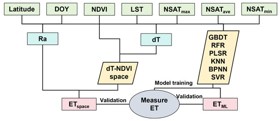
Figure 4.
The flowchart for estimating ET using the dT-NDVI method and machine learning methods.
4. Results
4.1. Validation of Long-Time-Series LST-VI Space Method
4.1.1. dT-NDVI Space Establishment
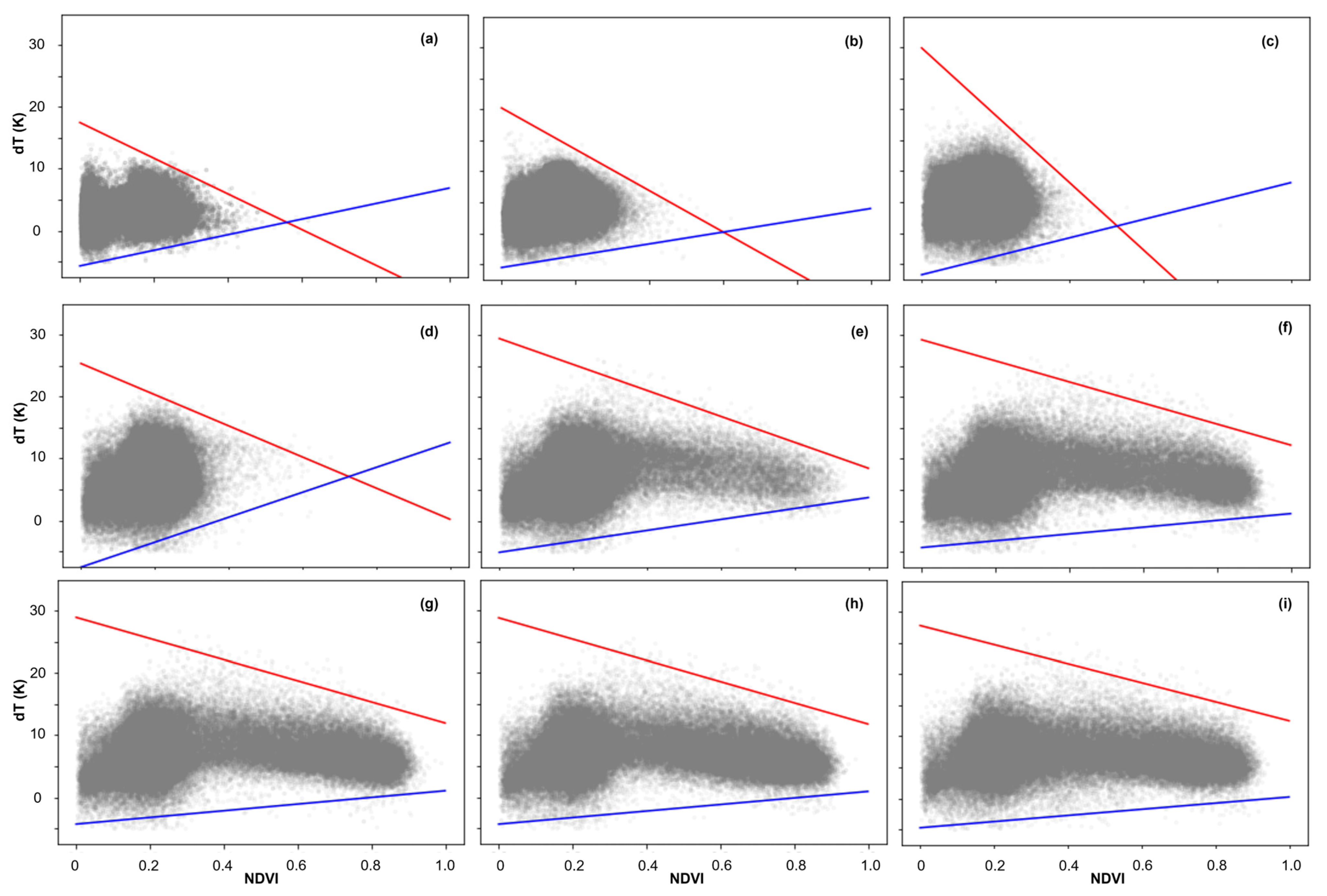
In this study, the dT-NDVI space evolves as the number of remote sensing images utilized changes, as depicted in Figure 5. The long-term series progressively increases with the number of images from DOY = 1 (Figure 5a) to DOY = 365 (Figure 5i). When fewer than 120 images are used, the dT-NDVI space adopts a triangular form, with NDVI values consistently remaining below 0.6 (Figure 5a–d). As the image count continues to rise, the upper NDVI limit ascends, and the dT-NDVI space gradually morphs into a trapezoidal shape (Figure 5e–i).
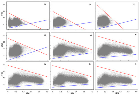
Figure 5.
The dT-NDVI space from different amounts of RS images: (a) 1 image; (b) 40 images; (c) 80 images; (d) 120 images; (e) 160 images; (f) 200 images; (g) 240 images; (h) 300 images; (i) 365 images. Note: the red lines indicate dry edges and blue lines indicate wet edges.
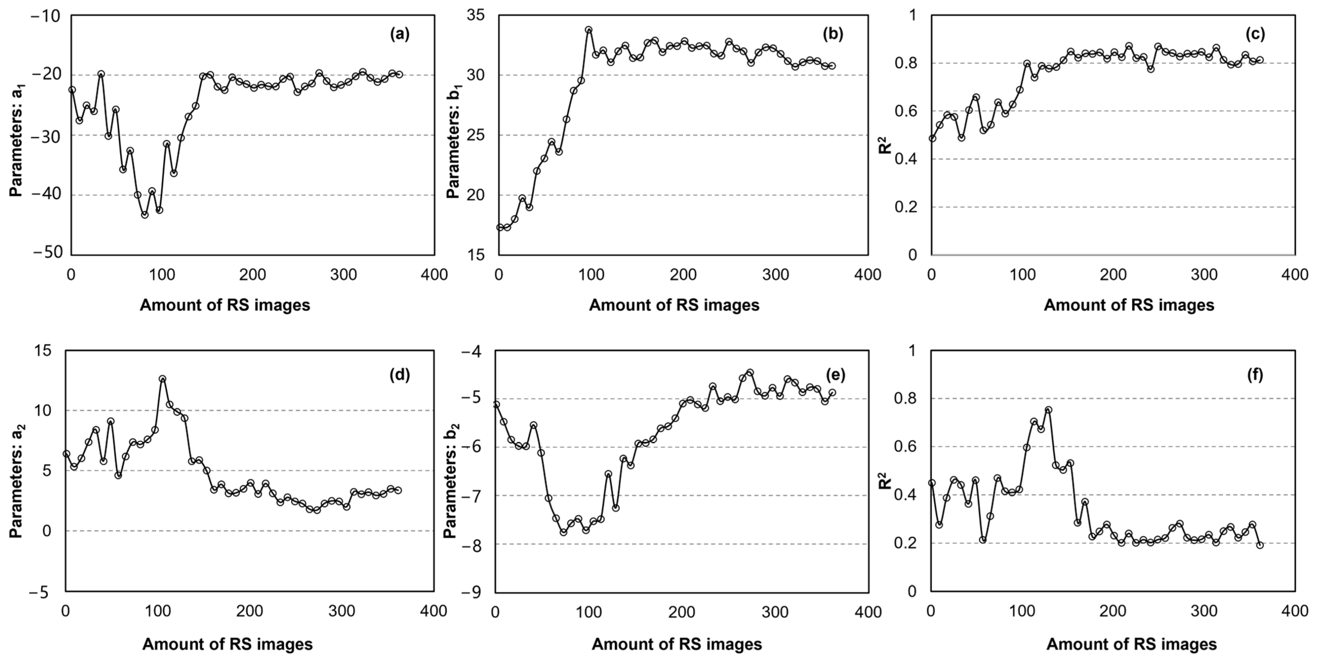
Figure 6 illustrates the variation in fitting parameters and accuracy in relation to the number of remote sensing images. For the dry edge (Figure 6a–c), a general decreasing trend is observed. After incorporating roughly 120 images, the fitting parameters stabilize, with a1 approximating −19 and b1 approximating 30, and the fitting accuracy also plateaus at an R2 of approximately 0.8. For the wet edge, the fitted line gradually shifts from an upward trend to a horizontal one. Following the use of approximately 160 images, a2 stabilizes at around 3 and b2 at around −5, with the fitting accuracy also stabilizing but at a lower R2, consistently below 0.3.
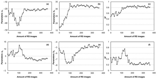
Figure 6.
Variation with amount of RS images of fitting parameters of dry edge—(a) a1, (b) b1, and accuracy (c) R2—and wet edge—(d) a1, (e) b1, and accuracy (f) R2.
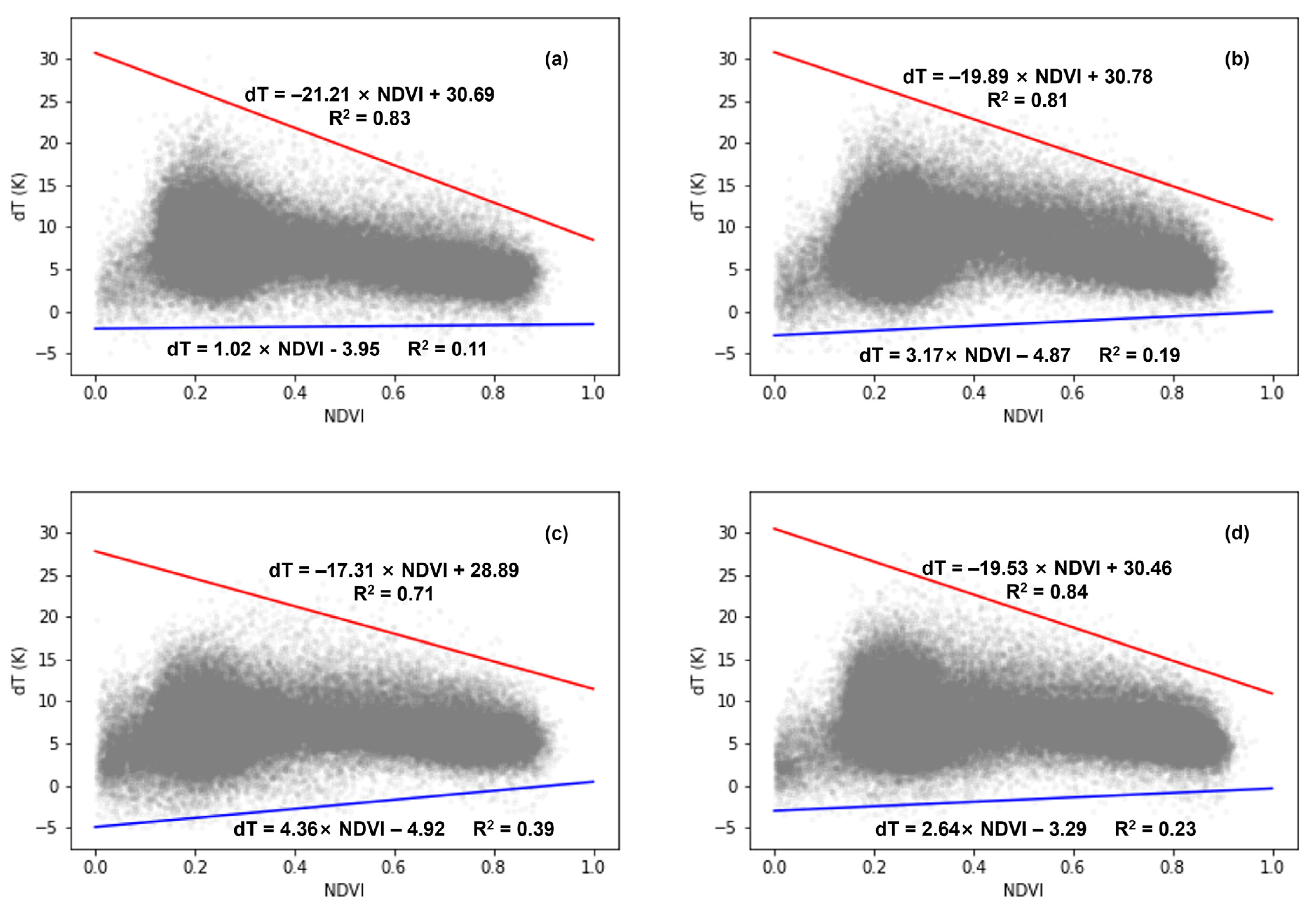
When comparing the dT-NDVI spatial patterns across different years using all the available images (Figure 7), a consistent trapezoidal shape is evident. The dry edges for the four years are in close proximity, with a1 ranging from −17.31 to −21.21 and b1 from 28.89 to 30.78. The fitting accuracy for the dry edge is high, with R2 values spanning from 0.71 to 0.83. Conversely, the fitting accuracy for the wet edge is relatively lower, with R2 values ranging from 0.11 to 0.39, albeit with similar parameters, where a2 ranges from 1.02 to 4.36 and b2 from −3.29 to −4.92. Overall, the dT-NDVI space constructed using long-term remote sensing data offers a more comprehensive portrayal of the extreme wet and dry conditions of vegetation and bare soil.
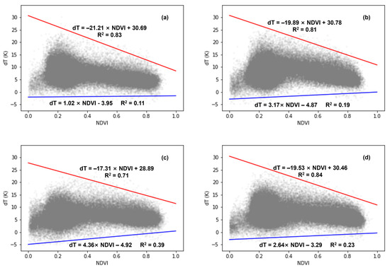
Figure 7.
The dT-NDVI space over different years: (a) 2008; (b) 2009; (c) 2010; (d) 2016. Note: the red lines indicate dry edges and blue lines indicate wet edges.
4.1.2. Accuracy of ET Estimation
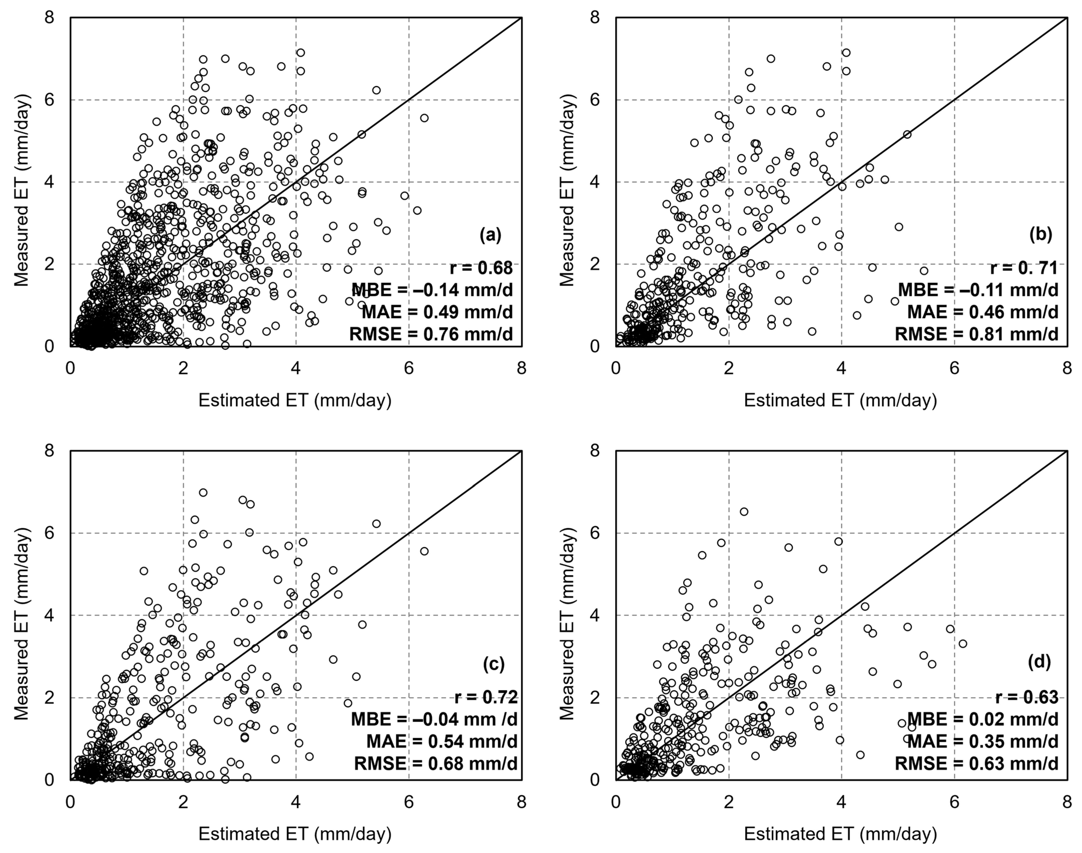
Figure 8 presents the results of ET estimation using the dT-NDVI space algorithm based on yearly long-time-series remote sensing images. The results revealed that the accuracy of ET estimation is characterized by a correlation coefficient (r) of 0.68, a root mean square error (RMSE) of 0.76 mm/d, a mean absolute error (MAE) of 0.49 mm/d, and a mean bias error (MBE) of −0.14 mm, indicating a slight underestimation (Figure 8a). Further comparisons were made of validation results from different sites: at DX, the validation results showed r = 0.71, RMSE = 0.81 mm/d, MAE = 0.46 mm/d, and MBE = −0.11 mm (Figure 8b); at HL, the results were r = 0.72, RMSE = 0.68 mm/d, MAE = 0.54 mm/d, and MBE = −0.04 mm (Figure 8c); and at MY, the results were r = 0.63, RMSE = 0.63 mm/d, MAE = 0.35 mm/d, and MBE = 0.02 mm (Figure 8d). The ET estimated based on the dT-NDVI spatial algorithm demonstrated better accuracy at forest sites compared to agricultural sites.

Figure 8.
The scatter of ET estimations based on the Ts-VI method: (a) all sites; (b) Daxing; (c) Huailai; (d) Miyun.
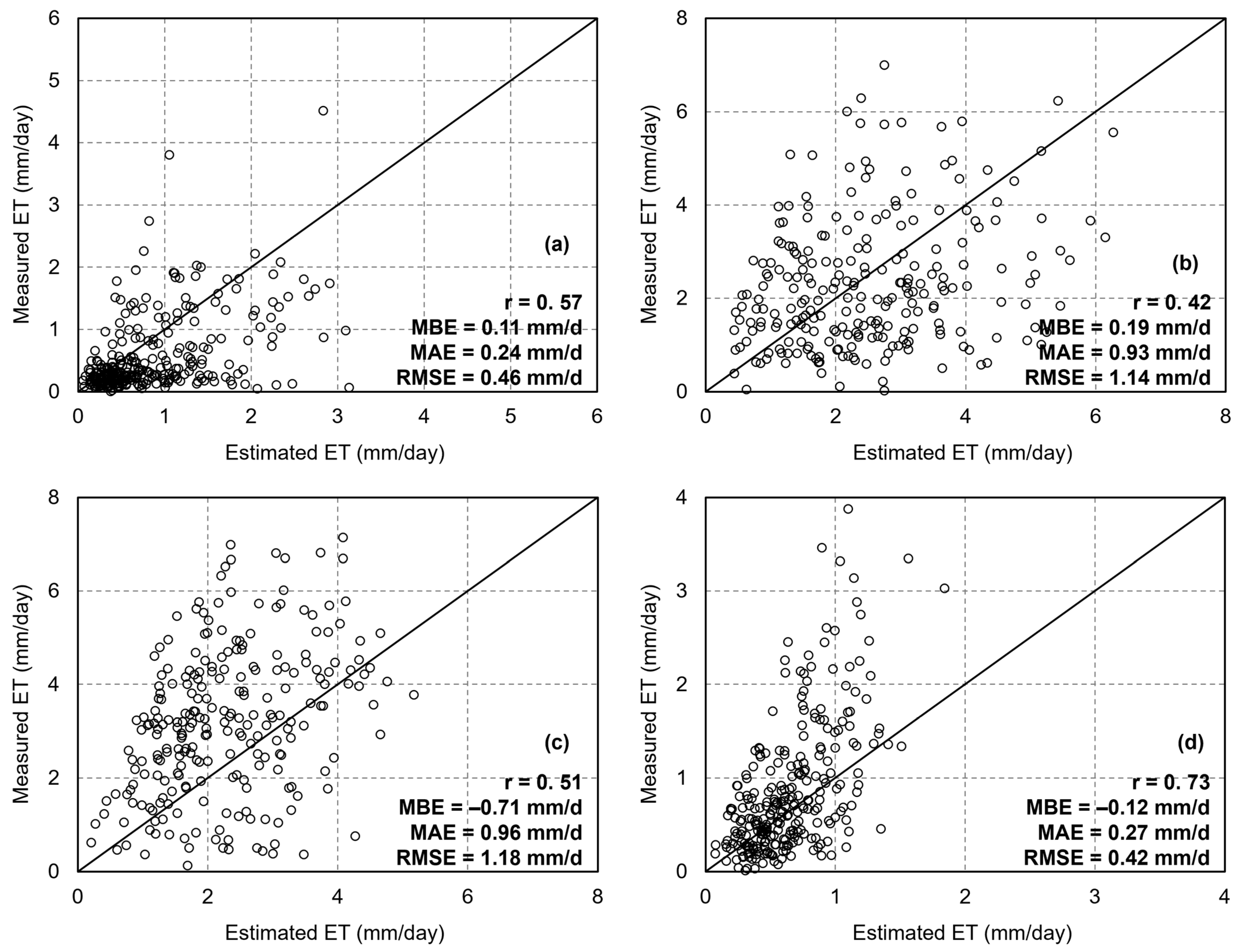
The accuracy of ET estimation across different seasons was also compared (Figure 9). For spring ET estimation, the dT-NDVI spatial algorithm achieved an accuracy of r = 0.57, RMSE = 0.16 mm/d, MAE = 0.14 mm/d, and MBE = 0.11 mm (Figure 9a); for summer, the accuracy was r = 0.42, RMSE = 1.14 mm/d, MAE = 0.93 mm/d, and MBE = 0.19 mm (Figure 9b); for autumn, the accuracy was r = 0.51, RMSE = 1.18 mm/d, MAE = 0.96 mm/d, and MBE = −0.71 mm (Figure 9c); and for winter, the accuracy was r = 0.73, RMSE = 0.42 mm/d, MAE = 0.27 mm/d, and MBE = −0.12 mm (Figure 9d). The dT-NDVI spatial method exhibited acceptable accuracy across all four seasons.

Figure 9.
The scatter of ET estimations based on the Ts-VI method in different seasons: (a) spring; (b) summer; (c) autumn; (d) winter.
4.2. Validation of Machine Learning Methods
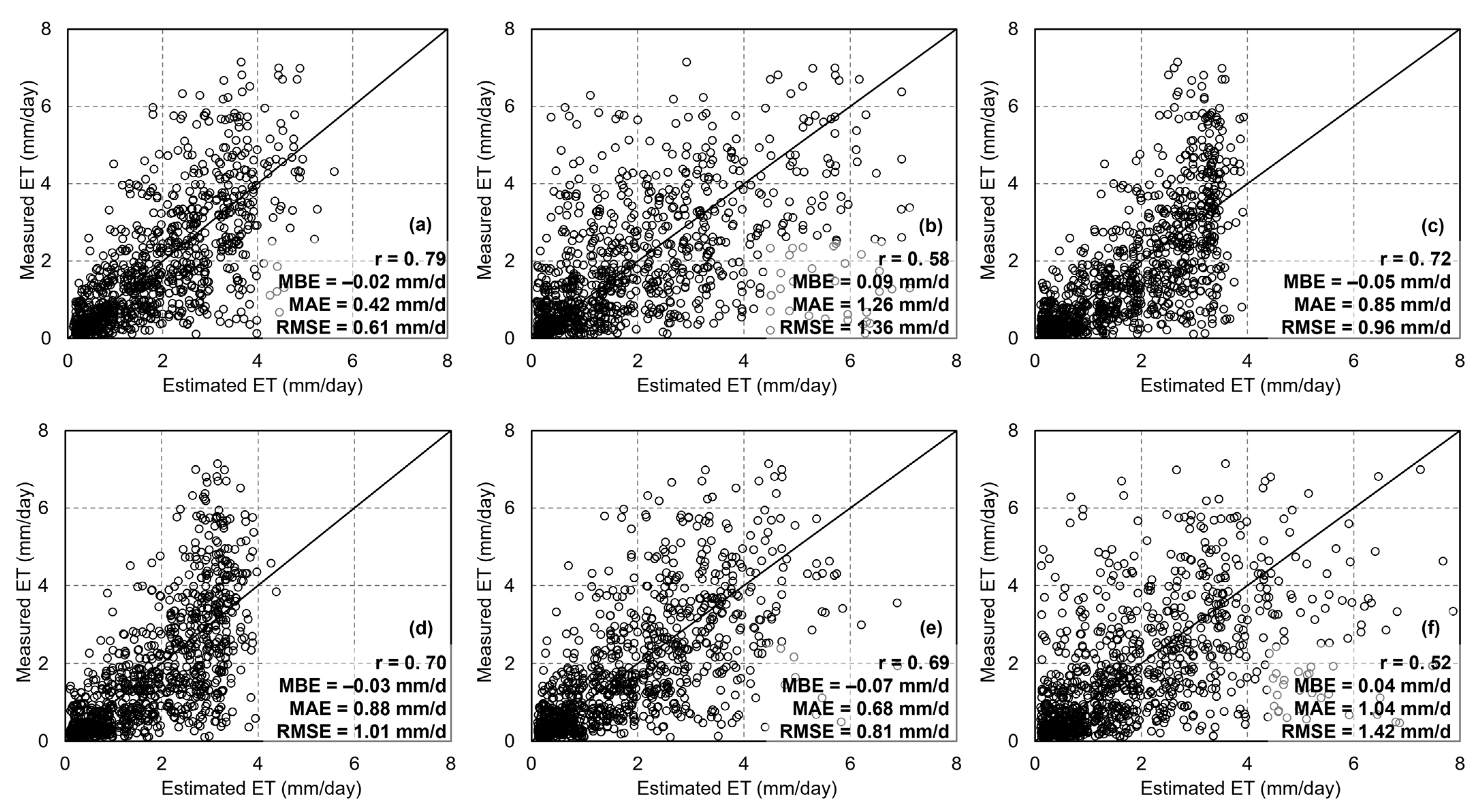
The five-fold cross-validation results for estimating ET using six machine learning algorithms are presented in Figure 10. Random Forest Regression (RFR) demonstrated the highest accuracy (r = 0.79, RMSE = 0.61 mm/d, MAE = 0.42 mm/d, and MBE = −0.02 mm, Figure 10a), followed by the BPN (r = 0.69, RMSE = 0.81 mm/d, MAE = 0.68 mm/d, and MBE = −0.07 mm, Figure 10e). Although the PLSR and KNN algorithms exhibited a certain level of accuracy, they both showed significant underestimation in high-value areas (Figure 10c,d), with accuracies of r = 0.72, RMSE = 0.96 mm/d, MAE = 0.85 mm/d, and MBE = −0.05 mm for PLSR, and r = 0.70, RMSE = 1.01 mm/d, MAE = 0.88 mm/d, and MBE = −0.03 mm for KNN. Despite being a typical ensemble learning algorithm like RFR, the GBDT method exhibited limited accuracy in estimating ET (r = 0.58, RMSE = 1.36 mm/d, MAE = 1.26 mm/d, and MBE = 0.09 mm, Figure 10b). Among the six machine learning algorithms, SVR performed the worst, with an accuracy of r = 0.52, RMSE = 1.42 mm/d, MAE = 1.04 mm/d, and MBE = 0.04 mm (Figure 10f). Overall, the performance of the machine learning algorithms was generally better than that of the dT-NDVI space-based method, with RFR being the most accurate algorithm.
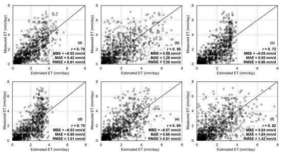
Figure 10.
The scatter of ET estimations using different algorithms: (a) Random Forest regression; (b) gradient boosting decision tree; (c) partial least square regression; (d) K-Nearest Neighbors; (e) backpropagation neural network; (f) support vector regression.
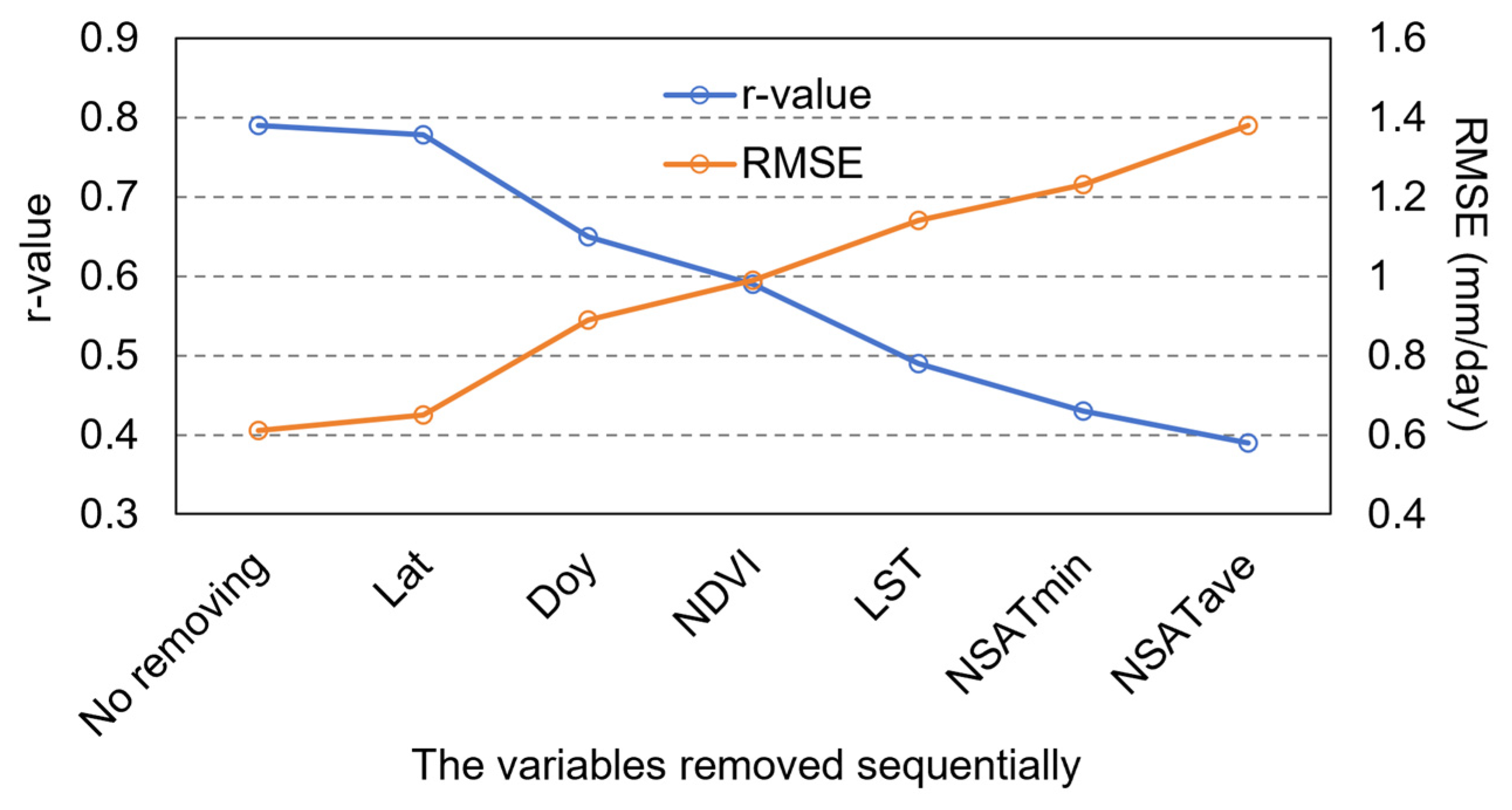
During the modeling process of the RFR, the importance of each input variable for estimating the target was assessed using the Gini index, as shown in Figure 11. The maximum near-surface air temperature exhibited the highest importance, followed by the average and minimum near-surface air temperatures. The importance of land surface temperature (LST) for ET estimation was lower than that of NSAT. The importance of NDVI, which represents vegetation growth, was lower than that of the four temperature variables. The importance of DOY and latitude was significantly lower compared to the other variables. Reducing the number of variable inputs into a machine learning model is one of the ways to improve model efficiency. We sequentially removed variables based on their importance, from lowest to highest, and analyzed the changes in accuracy. The results are shown in Figure 12. Besides latitude information (Lat), reducing the number of variable inputs gradually decreased the accuracy of ET estimation by the RFR. When only NSATmax (the most important variable) was used as input, the accuracy of ET estimation by RFR dropped to an r-value of 0.39 and an RMSE of 1.38 mm/day. Overall, compared to traditional energy balance models, the RFR model used in this study requires fewer input variables.
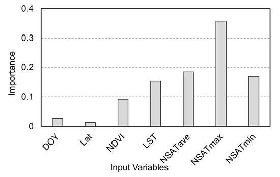
Figure 11.
The importance of different input variables in ET estimation using RFR.
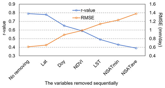
Figure 12.
The impact of reducing variable input on the accuracy of ET estimation by RFR.
Figure 13 presents the results of ET estimation using the RFR method at different sites: at DX, the validation results showed r = 0.73, RMSE = 0.68 mm/d, MAE = 0.41 mm/d, and MBE = −0.04 mm (Figure 13b); at HL, the results were r = 0.74, RMSE = 0.56 mm/d, MAE = 0.37 mm/d, and MBE = −0.01 mm (Figure 13c); and at MY, the results were r = 0.70, RMSE = 0.58 mm/d, MAE = 0.35 mm/d, and MBE = 0.01 mm (Figure 13d). The accuracy of the RFR algorithm is similar across different sites and higher than that of the dT-NDVI space method. Regarding the accuracy of the RFR algorithm across different seasons, the results show the following: for spring ET estimation, RFR achieved an accuracy of r = 0.79, RMSE = 0.19 mm/d, MAE = 0.15 mm/d, and MBE = 0.07 mm (Figure 14a); for summer, the accuracy was r = 0.71, RMSE = 0.71 mm/d, MAE = 0.51 mm/d, and MBE = −0.12 mm (Figure 14b); for autumn, the accuracy was r = 0.73, RMSE = 0.78 mm/d, MAE = 0.55 mm/d, and MBE = −0.22 mm (Figure 14c); and for winter, the accuracy was r = 0.69, RMSE = 0.42 mm/d, MAE = 0.25 mm/d, and MBE = 0.09 mm (Figure 14d). The RFR algorithm demonstrates a certain level of accuracy across all seasons. Compared to the dT-NDVI space method, it exhibits similar accuracy in spring and winter, whereas in summer and autumn, the RFR algorithm significantly outperforms the dT-NDVI space method in terms of accuracy. Overall, the RFR algorithm exhibits better and more stable accuracy in estimating ET across different scenarios compared to the dT-NDVI method.
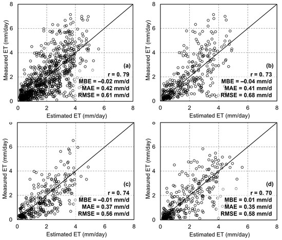
Figure 13.
The scatter of ET estimations based on RFR: (a) all sites; (b) Daxing; (c) Huailai; (d) Miyun.
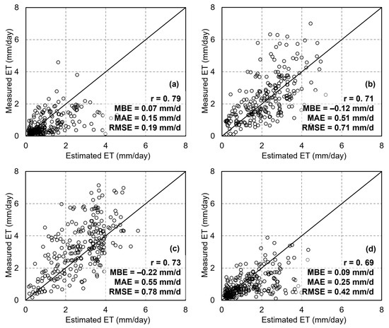
Figure 14.
The scatter of ET estimations based on RFR in different seasons: (a) spring; (b) summer; (c) autumn; (d) winter.
4.3. Spatial Analysis of ET Mapping
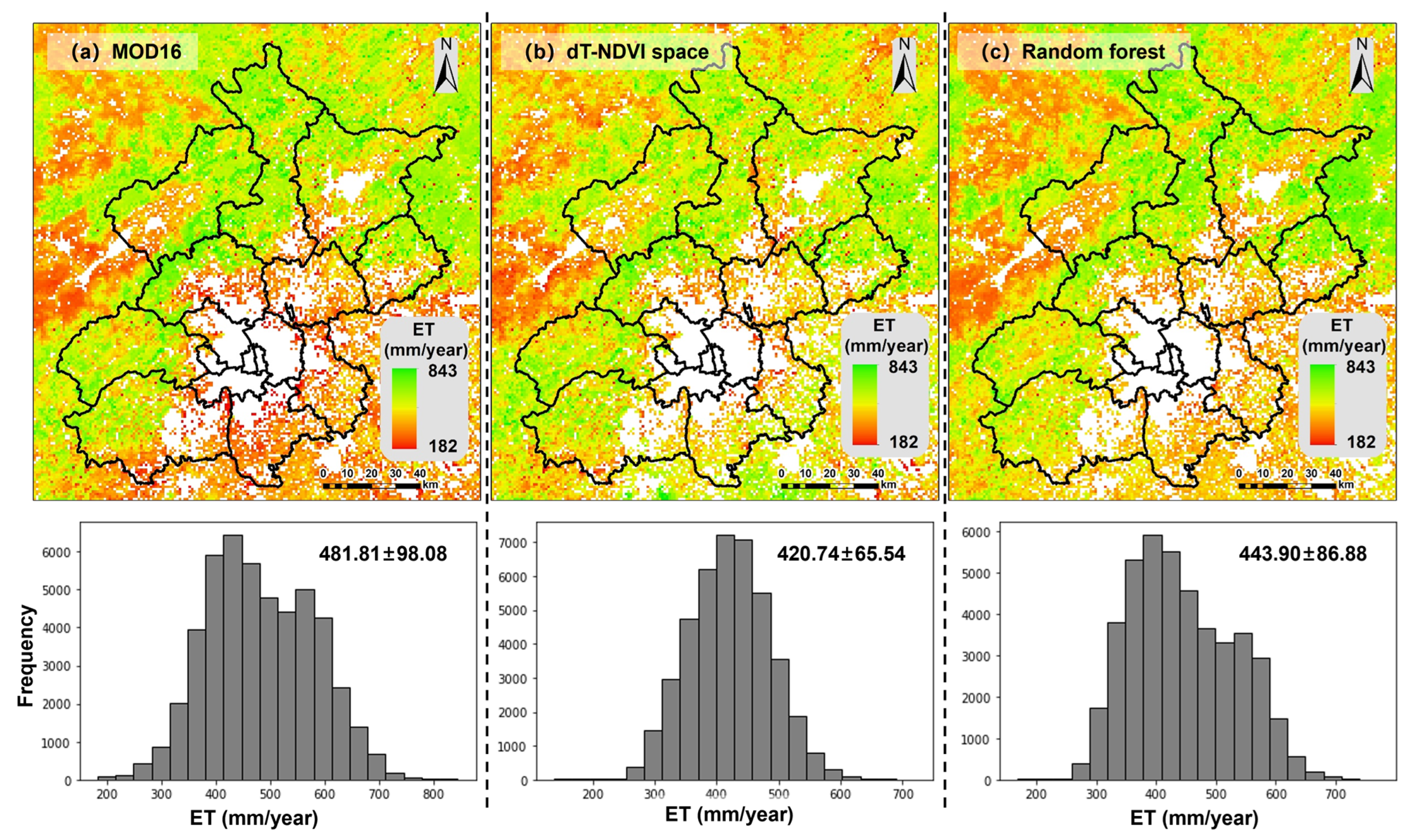
Figure 15 illustrates the spatial distribution of annual average evapotranspiration (ET) estimated by the algorithms based on the dT-NDVI space and Random Forest Regression (RFR), in comparison with MOD16 data. Overall, the three ET estimations exhibit similar spatial patterns, with higher values in the northwest and lower values in the southeast. Specifically, the algorithm based on the dT-NDVI space estimates an annual average ET of 420.74 ± 65.54 mm for the target region, while the RFR-based estimation yields an annual average ET of 443.90 ± 86.88 mm. Both results are lower than those provided by MOD16 (481.81 ± 98.08 mm), Moreover, this phenomenon is more pronounced in forestland (Figure 16b), where the estimated ET for the forest in the study area by MOD16 (551.33 ± 81.60 mm) is significantly higher than that estimated by RFR (489.94 ± 81.09 mm) and dT-NDVI space (443.37 ± 69.37 mm). In contrast, the ET estimates for cropland by the three methods are relatively close (Figure 16a, MOD16: 432.12 ± 67.06 mm; RFR: 409.45 ± 65.66 mm; dT-NDVI space: 399.39 ± 62.70 mm).
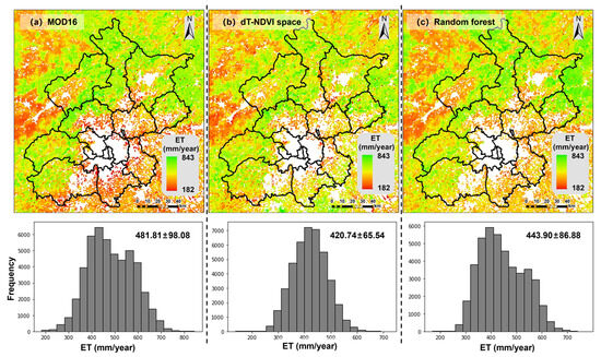
Figure 15.
The ET maps based on (a) MOD16, (b) the dT-NDVI space, and (c) Random Forest Regression.
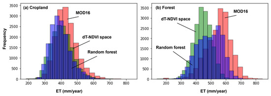
Figure 16.
The histogram of ET in (a) cropland and (b) forest.
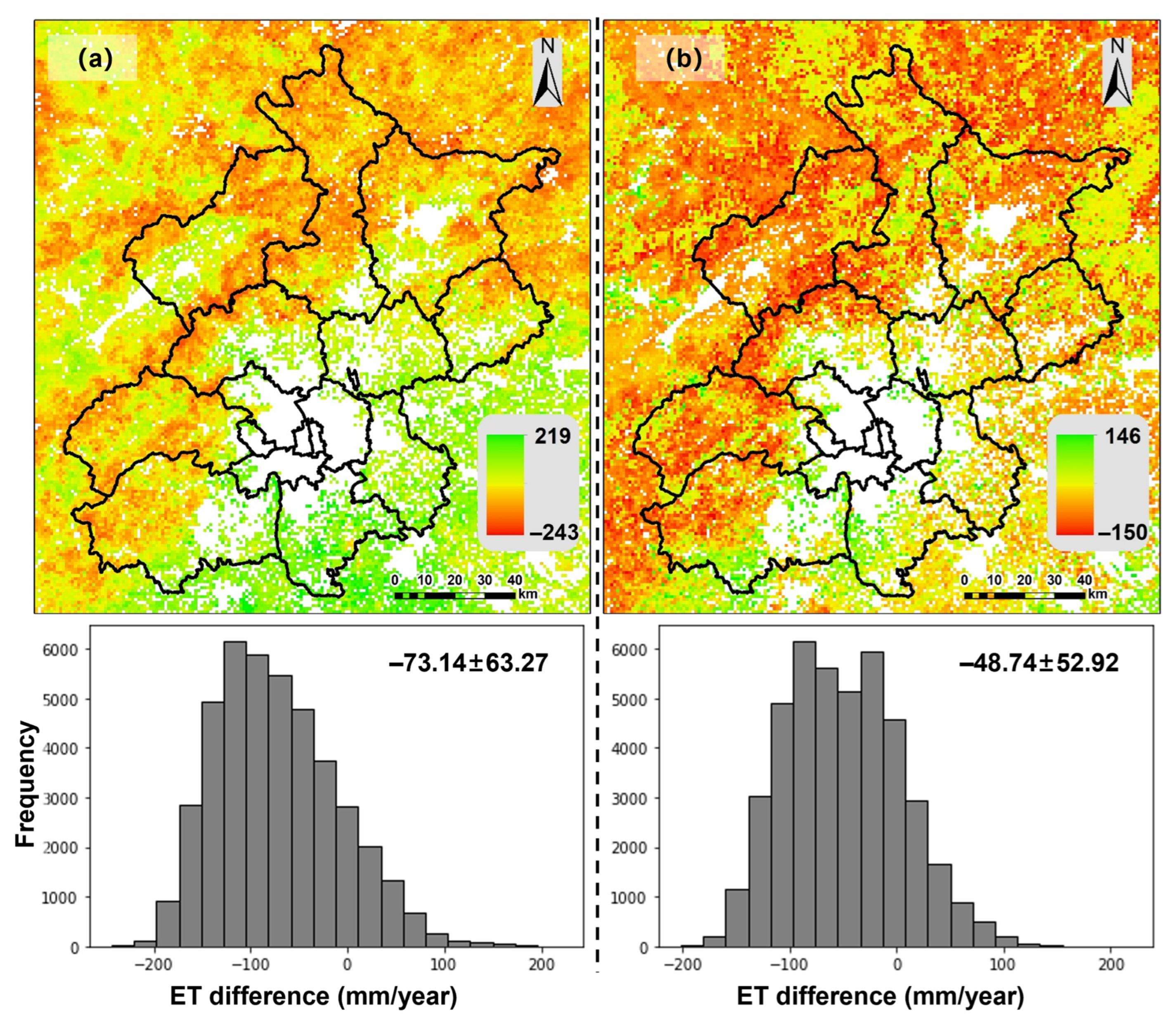
Figure 17 presents the distribution of differences between the annual average ET estimated by the dT-NDVI space-based algorithm and RFR, compared to MOD16. The ET estimated based on the dT-NDVI space is higher than MOD16 in the southeast region but lower in the northwest region, with an overall difference of −73.14 ± 63.27 mm compared to MOD16. Similarly, the ET estimated by RFR exhibits the same trend, being higher than MOD16 in the southeast and lower in the northwest. However, the overall difference is smaller compared to the dT-NDVI space-based estimation, with a difference of −48.74 ± 52.92 mm compared to MOD16.
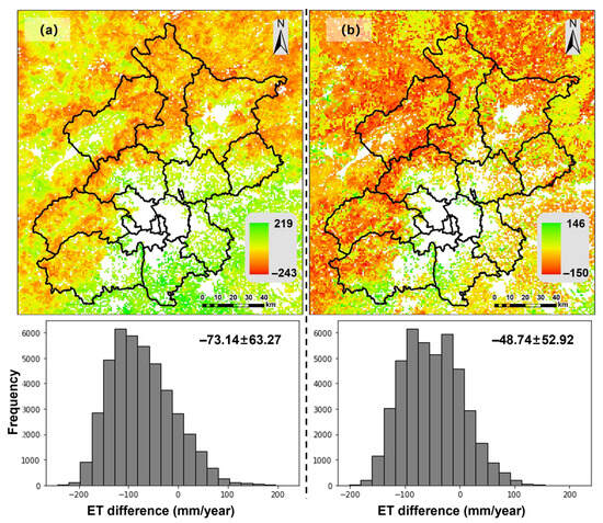
Figure 17.
The differences between the dT-NDVI space method-estimated ET (a) and RFR-estimated ET (b) and MOD16 ET, respectively.
5. Discussion
This study compared the accuracy of estimating evapotranspiration (ET) using the feature space method and six machine learning algorithms, and a thorough analysis was conducted on the temporal domain issues within the long-term-time-series feature space. The results indicate that the machine learning algorithm, Random Forest Regression (RFR), provides more accurate ET estimates. However, machine learning algorithms typically require a large number of prior samples to train the model, whereas the feature space method can directly estimate ET without prior samples and involves a simple calculation process. Therefore, the feature space method has more advantages in terms of broad application.
5.1. LST-NDVI Space Method
The basic assumption of the feature space is that under certain atmospheric forcing conditions, when vegetation cover or the vegetation index is fixed, surface temperature is determined by the soil or vegetation moisture content; conversely, when the soil or vegetation moisture content is fixed, surface temperature is determined by vegetation cover or the vegetation index [28]. The spatiotemporal variations in atmospheric forcing conditions can affect the reliability of the constructed feature space for the target area. Therefore, this study introduces air temperature and uses the difference between surface temperature and air temperature instead of surface temperature to construct the feature space [49,67]. Some studies have also proposed using air temperature as a separate dimension in the feature space to establish a three-dimensional feature space for estimating water conditions in the target area [41,68,69].
It is worth noting that the accuracy of the feature space in describing the extreme temperatures of the target area under certain atmospheric forcing conditions largely depends on the reasonableness of the target area’s scope (spatial domain), which introduces uncertainty into the feature space [38]. Cheng et al.’s [66] study on the wet and dry limits of the SEBAL model suggests that a range of 50 km × 50 km to 300 km × 300 km is a suitable spatial domain size. The target area in this study, approximately 230 km × 270 km, falls within this suitable range. For feature spaces established based on long-term remote sensing data, the temporal domain has rarely been discussed in previous studies. The results of this study (Figure 5) indicate that increasing the length of the remote sensing time series yields more stable wet/dry edge parameters compared to single-temporal remote sensing data, and the fitting parameters tend to stabilize after approximately 120 periods (Figure 6). This is because sufficient remote sensing data provides a more stable and comprehensive background field, allowing the feature space to adequately capture the extreme wet and dry conditions of bare soil and vegetation in the target area.
It is noteworthy that the feature space constructed through the scatter plot of dT (difference in temperature) and NDVI (Normalized Difference Vegetation Index) is susceptible to the influence of outliers, namely pseudo-wetness and -dryness points. As shown in Figure 18, these pseudo-points may arise from observation errors in the original remote sensing data (such as LST, NDVI, etc.) or deviations in the fitting of the wetness and dryness edges. Figure 6 illustrates that the dry edge in the feature space is fitted with high accuracy, whereas the accuracy of the wet edge is relatively unstable, which to some extent affects the estimation of ET (evapotranspiration). Nevertheless, the wet edge generally trends towards a horizontal line, and despite its low fitting accuracy, it has a relatively minor impact on ET estimation. Besides improving the accuracy of the original remote sensing data, some studies have proposed avoiding the influence of outliers by determining theoretical wetness and dryness limits [70,71]. However, this approach requires a substantial amount of meteorological observation data, thereby increasing the complexity of the feature space method. Furthermore, Hu et al. [72] suggested that the fitting accuracy of the wetness and dryness edges can be enhanced using nonlinear functions. However, the selection of nonlinear functions and their stability in ET estimation requires further study.
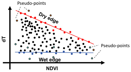
Figure 18.
Illustration of pseudo-wetness and dryness points in dT-NDVI space.
Additionally, potential evapotranspiration is a crucial factor in estimating ET using the feature space method. Although the Penman–Monteith model is widely used, it has the disadvantage of requiring numerous parameters. The Hargreaves–Samani (HS) model used in this study reduces the parameter requirements while maintaining a certain level of accuracy [56]. The results also indicate that the accuracy of the feature space method varies among different vegetation types, with forest sites exhibiting a slightly higher accuracy than agricultural ecosystem sites. Cheng et al.’s evaluation of the accuracy of the SEBAL model and the MOD16 model similarly revealed higher accuracy in the forestland [66]. For the feature space method, differences in water and thermal conditions among various vegetation types may be the primary reason for the accuracy discrepancies. Similarly, studies have indicated that there are significant differences in the correlations among land surface temperature, vegetation index, and air temperature across different vegetation types [73]. Therefore, some studies have proposed that feature spaces for different vegetation types should be constructed separately [28]. The study area, Beijing, China, is a typical semi-arid region. The wet and dry edges in the feature space essentially represent extreme drought and fully saturated conditions, which theoretically align well with semi-arid areas but are relatively less applicable to humid regions [66,74]. Hence, the applicability of the feature space method needs to be further enhanced from a theoretical perspective.
5.2. Machine Learning Method
Machine learning algorithms, benefiting from their powerful nonlinear fitting and data mining capabilities [36], have been widely applied to the construction of remote sensing models, such as crop yield estimation [75], crop growth assessment [76], and soil moisture estimation [77]. However, the applicability of different machine learning algorithms varies. The results of this study indicate that RFR provides the best ET estimates. As a typical ensemble learning algorithm, RFR obtains prediction results by averaging multiple decision trees, resulting in high model stability. Its excellent performance has also been demonstrated in other related studies [78,79]. Another ensemble learning algorithm, gradient boosting decision tree (GBDT), predicts results through a ’linear connection’ between decision trees, making the model susceptible to outliers [80]. The partial least square regression (PLSR) and K-Nearest Neighbors (KNN) algorithms perform poorly when dealing with complex nonlinear regression problems. Overall, while RFR demonstrates good accuracy, it is important to note that the portability of machine learning algorithms remains uncertain. Specifically, whether a trained model can be applied to other regions requires further investigation. Input variables are a crucial factor affecting the portability of machine learning models.
Input variables are critical factors that affect the portability and accuracy of machine learning models. In this study, only seven variables were selected as inputs for the model, which, compared to similar studies [48,81,82], has minimized model complexity and enhanced its efficiency to the greatest extent possible. Among these seven variables, NDVI is extensively employed to characterize vegetation growth [62,63]. However, traditional vegetation indices may be affected by spectral saturation effects, which can impair their ability to represent vegetation. Cheng et al. [74] utilized unmanned aerial vehicle (UAV)-borne LiDAR data to improve vegetation indices, significantly mitigating the impact of saturation effects. Nevertheless, for satellite remote sensing observations, further research is needed to develop vegetation indices with stronger resistance to saturation. LST can reflect the moisture status of the surface to some extent [64]. Both NDVI and LST have demonstrated a certain importance in estimating ET using RFR. NSAT represents atmospheric evaporation conditions [65], and the three NSAT metrics (maximum, average, and minimum values) exhibited the highest importance in RFR. Similarly, studies have shown that ET is most sensitive to air temperature [65], which is consistent with the findings of Cheng et al. [48]. This is because temperature provides key information such as radiative energy and surface moisture conditions. Theoretically, ET and air temperature interact with each other; as temperature rises, it promotes the transition of water from liquid to vapor, and water vapor has a cooling effect in the atmosphere [83]. Therefore, utilizing different types of temperature metrics (maximum, average, and minimum values) holds potential for improving ET estimation. Under extreme climate conditions, for the feature space method, the choice of method for calculating potential evapotranspiration may be critical to model accuracy [84], while for machine learning methods, sufficient observational samples under extreme conditions are needed to train a stable model. Time (day of year, DOY) and location (latitude, Lat) can directly reflect the intensity of solar radiation [66], but both variables showed relatively low importance, possibly because other variables (vegetation indices and temperatures) already encapsulate this information to some extent. Consequently, the accuracy of RFR remained high even after removing these two variables (Figure 12).
In summary, both machine learning methods and feature space methods can provide reliable ET estimates under conditions of limited observational variables. The feature space method is supported by certain physical mechanisms and does not require prior samples, offering greater potential for portability. Machine learning, on the other hand, can achieve higher accuracy but requires a large number of prior samples to train the model, and its applicability also carries uncertainties.
5.3. Comparison with Other Studies
Compared to the accuracy of other algorithms for estimating ET, for example, Cheng et al. [7] evaluated the accuracy of MOD16 ET data in China using tower observation data and found that the correlation coefficient (r) ranged from 0.69 to 0.95, with a root mean square error (RMSE) of 1.38–7.22 mm/8 days. Yang et al. [85] assessed the performance of GLEAM in China using data from eight flux towers and reported r-values ranging from 0.64 to 0.95 and RMSE values ranging from 7.72 to 29.76 mm/month. Furthermore, Li et al. [86] evaluated the performance of GLDAS in China using data from 12 flux towers and found that the r-value ranged from 0.73 to 0.98, with an RMSE of 14.93 to 35.17 mm/month. Cheng et al. [66] used eight flux towers’ observation data to evaluate the accuracy of SEBAL ET and MOD16 in China, with r and RMSE = 44.91% and 48.72%, respectively. Overall, these algorithms exhibit high accuracy but require numerous parameters, including data such as wind speed that are difficult to rasterize at a high resolution. In contrast, the two methods proposed in this study achieve comparable accuracy with only a few parameters, such as temperature and vegetation index.
5.4. Potential Errors and Prospectives
In summary, the two algorithms proposed in this study, the dT-NDVI feature space method and Random Forest Regression (RFR), can both effectively estimate ET with limited input variables. RFR provides more accurate estimates when prior samples are available, while the feature space method is suitable for situations where no prior samples are available. However, based on the validation results, these methods still exhibit considerable errors, which can be attributed to three main factors: (1) Regarding the models themselves, the assumptions underlying the dT-NDVI method and the pseudo-wet/dry pixel issues mentioned earlier are the primary sources of error. Although machine learning methods possess strong fitting capabilities, they rely on observed samples, and the completeness and absence of outliers in these samples can affect the accuracy of model training. (2) The inherent errors in input variables also contribute to the model’s inaccuracy, including uncertainties in the retrieval accuracy of land surface temperature and air temperature, as well as the ability of vegetation indices to represent vegetation growth status. (3) Uncertainties in the validation data, such as flux tower observations, which, despite being widely used as a benchmark for validating the accuracy of different models, still have errors ranging from 5% to 20% [87]. Additionally, the spatial coverage of flux tower observations is influenced by the height of sensor deployment and wind speed and direction, making it difficult to match with remote sensing pixels, especially for the coarse resolution (1 km × 1 km) used in this study [48]. Overall, there is still much to explore in the remote sensing estimation of evapotranspiration.
For the feature space method and machine learning method involved in this study, the following scientific questions identified in this study are worth further exploration: (1) Both the temporal and spatial domains can affect the feature space. Can the influence of these background fields be parameterized? (2) Given the differences in water and heat conditions among different vegetation types, what are the similarities and differences in the feature spaces of different vegetation types under the same background fields? (3) As an important input variable for the RFR algorithm, NSATs are simulated data based on remote sensing models rather than directly derived from remote sensing observations. How can an accurate NSAT dataset be constructed with limited input variables?
6. Conclusions
In this study, we evaluated the effectiveness of a long-time-series dT-NDVI space algorithm and machine learning algorithms in estimating evapotranspiration (ET) and its spatial distribution across Beijing and its surrounding regions in China, given a limited set of input variables. Validation was performed using ground flux observations, and the spatial distribution patterns of ET were compared against MOD16 ET data. The key findings of our study are as follows:
(1) Long-time-series remote sensing data offers a more comprehensive background for the dT-NDVI space, resulting in higher fitting accuracy for both wet and dry edges. This enables precise ET estimation with the following metrics: r = 0.68, RMSE = 0.76 mm/d, MAE = 0.49 mm/d, and MBE = −0.14 mm.
(2) Machine learning algorithms, particularly the Random Forest Regressor (RFR), generally provide more-accurate ET estimates. The RFR achieves the highest accuracy with the following metrics: r = 0.79, RMSE = 0.61 mm/d, MAE = 0.42 mm/d, and MBE = −0.02 mm.
(3) Both the ET estimates derived from the feature space algorithm and the machine learning algorithm exhibit spatial distribution patterns that are consistent with MOD16 ET data, further validating the effectiveness of these two approaches.
The findings of this study contribute to water resource management and offer a fresh perspective on remote sensing-based methods for ET estimation.
Author Contributions
Conceptualization, M.C. and D.S.; methodology, X.L.; software, H.Z.; validation, H.Z., Y.Q. and Y.R.; formal analysis, H.Z.; investigation, Z.Z.; resources, D.S.; data curation, Z.Z.; writing—original draft preparation, D.S.; writing—review and editing, M.C. and Y.L.; visualization, Z.Z.; supervision, M.C.; project administration, M.C.; funding acquisition, M.C. All authors have read and agreed to the published version of the manuscript.
Funding
This research was supported by the National Natural Science Foundation of China (Grant No. 42301366), the China Postdoctoral Science Foundation (Grant No. 2023M733001), and the Basic Research Program Natural Science Foundation of Jiangsu Province (Grant No. SBK2023043261).
Data Availability Statement
The raw data supporting the conclusions of this article will be made available by the authors on request.
Conflicts of Interest
The authors declare no conflict of interest.
References
- Zhang, K.; Chen, H.; Ma, N.; Shang, S.; Wang, Y.; Xu, Q.; Zhu, G. A global dataset of terrestrial evapotranspiration and soil moisture dynamics from 1982 to 2020. Sci. Data 2024, 11, 445. [Google Scholar] [CrossRef] [PubMed]
- Zhang, K.; Zhu, G.; Ma, J.; Yang, Y.; Shang, S.; Gu, C. Parameter Analysis and Estimates for the MODIS Evapotranspiration Algorithm and Multiscale Verification. Water Resour. Res. 2019, 55, 2211–2231. [Google Scholar] [CrossRef]
- Amani, S.; Shafizadeh-Moghadam, H. A review of machine learning models and influential factors for estimating evapotranspiration using remote sensing and ground-based data. Agric. Water Manag. 2023, 284, 108324. [Google Scholar] [CrossRef]
- Jaafar, H.H.; Sujud, L.H. High-resolution satellite imagery reveals a recent accelerating rate of increase in land evapotranspiration. Remote Sens. Environ. 2024, 315, 114489. [Google Scholar] [CrossRef]
- Li, J.; Li, Y.; Yin, L.; Zhao, Q. A novel composite drought index combining precipitation, temperature and evapotranspiration used for drought monitoring in the Huang-Huai-Hai Plain. Agric. Water Manag. 2024, 291, 108626. [Google Scholar] [CrossRef]
- Callejas-Rodelas, J.Á.; Knohl, A.; van Ramshorst, J.; Mammarella, I.; Markwitz, C. Comparison between lower-cost and conventional eddy covariance setups for CO2 and evapotranspiration measurements above monocropping and agroforestry systems. Agric. For. Meteorol. 2024, 354, 110086. [Google Scholar] [CrossRef]
- Cheng, M.; Jiao, X.; Jin, X.; Li, B.; Liu, K.; Shi, L. Satellite time series data reveal interannual and seasonal spatiotemporal evapotranspiration patterns in China in response to effect factors. Agric. Water Manag. 2021, 255, 107046. [Google Scholar] [CrossRef]
- Tran, B.N.; Van Der Kwast, J.; Seyoum, S.; Uijlenhoet, R.; Jewitt, G.; Mul, M. Uncertainty assessment of satellite remote-sensing-based evapotranspiration estimates: A systematic review of methods and gaps. Hydrol. Earth Syst. Sci. 2023, 27, 4505–4528. [Google Scholar] [CrossRef]
- Jaafar, H.H.; Ahmad, F.A. Time series trends of Landsat-based ET using automated calibration in METRIC and SEBAL: The Bekaa Valley, Lebanon. Remote Sens. Environ. 2020, 238, 111034. [Google Scholar] [CrossRef]
- Anderson, M.C.; Kustas, W.P.; Norman, J.M.; Diak, G.T.; Hain, C.R.; Gao, F.; Yang, Y.; Knipper, K.R.; Xue, J.; Yang, Y. A brief history of the thermal IR-based Two-Source Energy Balance (TSEB) model–diagnosing evapotranspiration from plant to global scales. Agric. For. Meteorol. 2024, 350, 109951. [Google Scholar] [CrossRef]
- Hu, X.; Shi, L.; Lin, G.; Lin, L. Comparison of physical-based, data-driven and hybrid modeling approaches for evapotranspiration estimation. J. Hydrol. 2021, 601, 126592. [Google Scholar] [CrossRef]
- Zhu, W.; Shi, X.; Wei, J. A universal triangle method for evapotranspiration estimation with MODIS products and routine meteorological observations: Algorithm development and global validation. Agric. Water Manag. 2024, 302, 109017. [Google Scholar] [CrossRef]
- Wang, S.; Wang, C.; Zhang, C.; Xue, J.; Wang, P.; Wang, X.; Wang, W.; Zhang, X.; Li, W.; Huang, G. A classification-based spatiotemporal adaptive fusion model for the evaluation of remotely sensed evapotranspiration in heterogeneous irrigated agricultural area. Remote Sens. Environ. 2022, 273, 112962. [Google Scholar] [CrossRef]
- Ma, Y.; Sun, S.; Li, C.; Zhao, J.; Li, Z.; Jia, C. Estimation of regional actual evapotranspiration based on the improved SEBAL model. J. Hydrol. 2023, 619, 129283. [Google Scholar] [CrossRef]
- Jiang, Y.; Tang, R.; Li, Z.-L. A framework of correcting the angular effect of land surface temperature on evapotranspiration estimation in single-source energy balance models. Remote Sens. Environ. 2022, 283, 113306. [Google Scholar] [CrossRef]
- Gowda, P.H.; Chávez, J.L.; Howell, T.A.; Marek, T.H.; New, L.L. Surface energy balance based evapotranspiration mapping in the Texas high plains. Sensors 2008, 8, 5186–5201. [Google Scholar] [CrossRef] [PubMed]
- Allen, R.G.; Tasumi, M.; Morse, A.; Trezza, R.; Wright, J.L.; Bastiaanssen, W.; Kramber, W.; Lorite, I.; Robison, C.W. Satellite-based energy balance for mapping evapotranspiration with internalized calibration (METRIC)—Applications. J. Irrig. Drain. Eng. 2007, 133, 395–406. [Google Scholar] [CrossRef]
- Su, Z. The Surface Energy Balance System (SEBS) for estimation of turbulent heat fluxes. Hydrol. Earth Syst. Sci. 2002, 6, 85–100. [Google Scholar] [CrossRef]
- Anderson, M.C.; Norman, J.M.; Mecikalski, J.R.; Torn, R.D.; Kustas, W.P.; Basara, J.B. A multiscale remote sensing model for disaggregating regional fluxes to micrometeorological scales. J. Hydrometeorol. 2004, 5, 343–363. [Google Scholar] [CrossRef]
- Norman, J.M.; Kustas, W.P.; Humes, K.S. Source approach for estimating soil and vegetation energy fluxes in observations of directional radiometric surface temperature. Agric. For. Meteorol. 1995, 77, 263–293. [Google Scholar] [CrossRef]
- Chang, Y.; Qin, D.; Ding, Y.; Zhao, Q.; Zhang, S. A modified MOD16 algorithm to estimate evapotranspiration over alpine meadow on the Tibetan Plateau, China. J. Hydrol. 2018, 561, 16–30. [Google Scholar] [CrossRef]
- Xie, Z.; Yao, Y.; Tang, Q.; Liu, M.; Fisher, J.B.; Chen, J.; Zhang, X.; Jia, K.; Li, Y.; Shang, K. Evaluation of seven satellite-based and two reanalysis global terrestrial evapotranspiration products. J. Hydrol. 2024, 630, 130649. [Google Scholar] [CrossRef]
- Li, X.; Xue, F.; Ding, J.; Xu, T.; Song, L.; Pang, Z.; Wang, J.; Xu, Z.; Ma, Y.; Lu, Z. A Hybrid Model Coupling Physical Constraints and Machine Learning to Estimate Daily Evapotranspiration in the Heihe River Basin. Remote Sens. 2024, 16, 2143. [Google Scholar] [CrossRef]
- Zoratipour, E.; Mohammadi, A.S.; Zoratipour, A. Evaluation of SEBS and SEBAL algorithms for estimating wheat evapotranspiration (case study: Central areas of Khuzestan province). Appl. Water Sci. 2023, 13, 137. [Google Scholar] [CrossRef]
- Kamyab, A.D.; Mokhtari, S.; Jafarinia, R. A comparative study in quantification of maize evapotranspiration for Iranian maize farm using SEBAL and METRIC-1 EEFLux algorithms. Acta Geophys. 2022, 70, 319–332. [Google Scholar] [CrossRef]
- Adem, E.; Boteva, S.; Zhang, L.; Elhag, M. Estimation of evapotranspiration based on METRIC and SEBAL model using remote sensing, near Al-Jouf, Saudi Arabia. Desalination Water Treat. 2023, 290, 94–103. [Google Scholar] [CrossRef]
- Derardja, B.; Khadra, R.; Abdelmoneim, A.A.; El-Shirbeny, M.A.; Valsamidis, T.; De Pasquale, V.; Deflorio, A.M.; Volden, E. Advancements in Remote Sensing for Evapotranspiration Estimation: A Comprehensive Review of Temperature-Based Models. Remote Sens. 2024, 16, 1927. [Google Scholar] [CrossRef]
- Tang, R.; Wang, S.; Jiang, Y.; Li, Z.; Liu, M.; Tang, B.; Wu, H. National Remote Sensing Bulletin. A review of retrieval of land surface evapotranspiration based on remotely sensed surface temperature versus vegetation index triangular/trapezoidal characteristic space. Nat. Remote Sens. Bull. 2021, 25, 65–82. [Google Scholar] [CrossRef]
- Nguyen, N.M.; Choi, M. Evapotranspiration partitioning and agricultural drought quantification with an optical trapezoidal framework. Agric. For. Meteorol. 2023, 338, 109520. [Google Scholar] [CrossRef]
- Hu, X.; Shi, L.; Lin, L.; Zhang, B.; Zha, Y. Optical-based and thermal-based surface conductance and actual evapotranspiration estimation, an evaluation study in the North China Plain. Agric. For. Meteorol. 2018, 263, 449–464. [Google Scholar] [CrossRef]
- Hasan, M.A.; Mia, M.B.; Khan, M.R.; Alam, M.J.; Chowdury, T.; Al Amin, M.; Ahmed, K.M.U. Temporal changes in land cover, land surface temperature, soil moisture, and evapotranspiration using remote sensing techniques—A case study of Kutupalong Rohingya Refugee Camp in Bangladesh. J. Geovisualization Spat. Anal. 2023, 7, 11. [Google Scholar] [CrossRef]
- Tang, R.; Li, Z.-L. An end-member-based two-source approach for estimating land surface evapotranspiration from remote sensing data. IEEE Trans. Geosci. Remote Sens. 2017, 55, 5818–5832. [Google Scholar] [CrossRef]
- Tang, R.; Li, Z.-L. Evaluation of two end-member-based models for regional land surface evapotranspiration estimation from MODIS data. Agric. For. Meteorol. 2015, 202, 69–82. [Google Scholar] [CrossRef]
- Guzinski, R.; Nieto, H.; Sandholt, I.; Karamitilios, G. Modelling high-resolution actual evapotranspiration through Sentinel-2 and Sentinel-3 data fusion. Remote Sens. 2020, 12, 1433. [Google Scholar] [CrossRef]
- Elkatoury, A.; Alazba, A.A.; Radwan, F.; Kayad, A.; Mossad, A. Evapotranspiration Estimation Assessment Using Various Satellite-Based Surface Energy Balance Models in Arid Climates. Earth Syst. Environ. 2024, 8, 1347–1369. [Google Scholar] [CrossRef]
- Cheng, M.; Jiao, X.; Liu, Y.; Shao, M.; Yu, X.; Bai, Y.; Wang, Z.; Wang, S.; Tuohuti, N.; Liu, S. Estimation of soil moisture content under high maize canopy coverage from UAV multimodal data and machine learning. Agric. Water Manag. 2022, 264, 107530. [Google Scholar] [CrossRef]
- Yin, B.; Li, Z.; Yue, R.; Lv, S.; Li, F. Monitoring drought in Guanzhong areas using temperature-vegetation drought index. Trans. Chin. Soc. Agric. Eng. 2024, 40, 111–119. [Google Scholar]
- Feng, J.; Wang, Z. A satellite-based energy balance algorithm with reference dry and wet limits. Int. J. Remote Sens. 2013, 34, 2925–2946. [Google Scholar] [CrossRef]
- Martínez Pérez, J.Á.; García-Galiano, S.G.; Martin-Gorriz, B.; Baille, A. Satellite-based method for estimating the spatial distribution of crop evapotranspiration: Sensitivity to the Priestley-Taylor coefficient. Remote Sens. 2017, 9, 611. [Google Scholar] [CrossRef]
- Przeździecki, K.; Zawadzki, J.J.; Urbaniak, M.; Ziemblińska, K.; Miatkowski, Z. Using temporal variability of land surface temperature and normalized vegetation index to estimate soil moisture condition on forest areas by means of remote sensing. Ecol. Indic. 2023, 148, 110088. [Google Scholar] [CrossRef]
- Cheng, M.; Sun, C.; Nie, C.; Liu, S.; Yu, X.; Bai, Y.; Liu, Y.; Meng, L.; Jia, X.; Liu, Y. Evaluation of UAV-based drought indices for crop water conditions monitoring: A case study of summer maize. Agric. Water Manag. 2023, 287, 108442. [Google Scholar] [CrossRef]
- Tang, R.; Li, Z.-L.; Liu, M.; Jiang, Y.; Peng, Z. A moisture-based triangle approach for estimating surface evaporative fraction with time-series of remotely sensed data. Remote Sens. Environ. 2022, 280, 113212. [Google Scholar] [CrossRef]
- Mohseni, F.; Mokhtarzade, M. A new soil moisture index driven from an adapted long-term temperature-vegetation scatter plot using MODIS data. J. Hydrol. 2020, 581, 124420. [Google Scholar] [CrossRef]
- Babaeian, E.; Sadeghi, M.; Franz, T.E.; Jones, S.; Tuller, M. Mapping soil moisture with the OPtical TRApezoid Model (OPTRAM) based on long-term MODIS observations. Remote Sens. Environ. 2018, 211, 425–440. [Google Scholar] [CrossRef]
- Zhu, W.; Jia, S.; Lv, A. A time domain solution of the Modified Temperature Vegetation Dryness Index (MTVDI) for continuous soil moisture monitoring. Remote Sens. Environ. 2017, 200, 1–17. [Google Scholar] [CrossRef]
- Zhu, W.; Jia, S.; Lv, A. A universal Ts-VI triangle method for the continuous retrieval of evaporative fraction from MODIS products. J. Geophys. Res. Atmos. 2017, 122, 10–206. [Google Scholar] [CrossRef]
- Carter, C.; Liang, S. Evaluation of ten machine learning methods for estimating terrestrial evapotranspiration from remote sensing. Int. J. Appl. Earth Obs. Geoinf. 2019, 78, 86–92. [Google Scholar] [CrossRef]
- Cheng, M.; Liu, K.; Liu, Z.; Xu, J.; Zhang, Z.; Sun, C. Combination of Multiple Variables and Machine Learning for Regional Cropland Water and Carbon Fluxes Estimation: A Case Study in the Haihe River Basin. Remote Sens. 2024, 16, 3280. [Google Scholar] [CrossRef]
- Wang, S.; Garcia, M.; Bauer-Gottwein, P.; Jakobsen, J.; Zarco-Tejada, P.J.; Bandini, F.; Paz, V.S.; Ibrom, A. High spatial resolution monitoring land surface energy, water and CO2 fluxes from an Unmanned Aerial System. Remote Sens. Environ. 2019, 229, 14–31. [Google Scholar] [CrossRef]
- Zhou, J.; Zhang, X.; Zhan, W.; Göttsche, F.-M.; Liu, S.; Olesen, F.-S.; Hu, W.; Dai, F. A thermal sampling depth correction method for land surface temperature estimation from satellite passive microwave observation over barren land. IEEE Trans. Geosci. Remote Sens. 2017, 55, 4743–4756. [Google Scholar] [CrossRef]
- Zhang, X.; Zhou, J.; Göttsche, F.-M.; Zhan, W.; Liu, S.; Cao, R. A method based on temporal component decomposition for estimating 1-km all-weather land surface temperature by merging satellite thermal infrared and passive microwave observations. IEEE Trans. Geosci. Remote Sens. 2019, 57, 4670–4691. [Google Scholar] [CrossRef]
- Zhang, X.; Zhou, J.; Liang, S.; Wang, D. A practical reanalysis data and thermal infrared remote sensing data merging (RTM) method for reconstruction of a 1-km all-weather land surface temperature. Remote Sens. Environ. 2021, 260, 112437. [Google Scholar] [CrossRef]
- Cheng, M.; Jin, X.; Sun, C.; Jiao, X.; Zhang, Z.; Liu, K. Nsatdc: Near Surface Air Temperature Dataset for China with High Temporal and Spatial Resolution Generated Using Random Forest and Multi-Source Data. SSRN 2024. Preprint. [Google Scholar] [CrossRef]
- Mu, Q.; Heinsch, F.A.; Zhao, M.; Running, S.W. Development of a global evapotranspiration algorithm based on MODIS and global meteorology data. Remote Sens. Environ. 2007, 111, 519–536. [Google Scholar] [CrossRef]
- Mu, Q.; Zhao, M.; Running, S.W. Improvements to a MODIS global terrestrial evapotranspiration algorithm. Remote Sens. Environ. 2011, 115, 1781–1800. [Google Scholar] [CrossRef]
- Song, Y.H.; Chung, E.-S.; Shahid, S. Global future potential evapotranspiration signal using Penman-Monteith and Hargreaves-Samani method by latitudes based on CMIP6. Atmos. Res. 2024, 304, 107367. [Google Scholar] [CrossRef]
- Ali, I.; Greifeneder, F.; Stamenkovic, J.; Neumann, M.; Notarnicola, C. Review of machine learning approaches for biomass and soil moisture retrievals from remote sensing data. Remote Sens. 2015, 7, 16398–16421. [Google Scholar] [CrossRef]
- Muruganantham, P.; Wibowo, S.; Grandhi, S.; Samrat, N.H.; Islam, N. A systematic literature review on crop yield prediction with deep learning and remote sensing. Remote Sens. 2022, 14, 1990. [Google Scholar] [CrossRef]
- Meraj, G.; Kanga, S.; Ambadkar, A.; Kumar, P.; Singh, S.K.; Farooq, M.; Johnson, B.A.; Rai, A.; Sahu, N. Assessing the yield of wheat using satellite remote sensing-based machine learning algorithms and simulation modeling. Remote Sens. 2022, 14, 3005. [Google Scholar] [CrossRef]
- Chen, Q.; Zheng, B.; Chenu, K.; Hu, P.; Chapman, S.C. Unsupervised plot-scale LAI phenotyping via UAV-based imaging, modelling, and machine learning. Plant Phenomics 2022, 2022, 9768253. [Google Scholar] [CrossRef]
- Chatterjee, S.; Baath, G.S.; Sapkota, B.R.; Flynn, K.C.; Smith, D.R. Enhancing LAI estimation using multispectral imagery and machine learning: A comparison between reflectance-based and vegetation indices-based approaches. Comput. Electron. Agric. 2025, 230, 109790. [Google Scholar] [CrossRef]
- Maselli, F.; Chiesi, M.; Angeli, L.; Fibbi, L.; Rapi, B.; Romani, M.; Sabatini, F.; Battista, P. An improved NDVI-based method to predict actual evapotranspiration of irrigated grasses and crops. Agric. Water Manag. 2020, 233, 106077. [Google Scholar] [CrossRef]
- Joiner, J.; Yoshida, Y.; Anderson, M.; Holmes, T.; Hain, C.; Reichle, R.; Koster, R.; Middleton, E.; Zeng, F.-W. Global relationships among traditional reflectance vegetation indices (NDVI and NDII), evapotranspiration (ET), and soil moisture variability on weekly timescales. Remote Sens. Environ. 2018, 219, 339–352. [Google Scholar] [CrossRef]
- Jiang, Y.; Weng, Q. Estimation of hourly and daily evapotranspiration and soil moisture using downscaled LST over various urban surfaces. GIScience Remote Sens. 2017, 54, 95–117. [Google Scholar] [CrossRef]
- Tabari, H.; Talaee, P.H. Sensitivity of evapotranspiration to climatic change in different climates. Glob. Planet. Chang. 2014, 115, 16–23. [Google Scholar] [CrossRef]
- Cheng, M.; Jiao, X.; Li, B.; Yu, X.; Shao, M.; Jin, X. Long time series of daily evapotranspiration in China based on the SEBAL model and multisource images and validation. Earth Syst. Sci. Data 2021, 13, 3995–4017. [Google Scholar] [CrossRef]
- Sebbar, B.-e.; Malbéteau, Y.; Khabba, S.; Bouchet, M.; Simonneaux, V.; Chehbouni, A.; Merlin, O. Estimating evapotranspiration in mountainous water-limited regions from thermal infrared data: Comparison of two approaches based on energy balance and evaporative fraction. Remote Sens. Environ. 2024, 315, 114481. [Google Scholar] [CrossRef]
- Chen, H.; Chen, H.; Zhang, S.; Chen, S.; Cen, F.; Zhao, Q.; Huang, X.; He, T.; Gao, Z. Comparison of CWSI and Ts-Ta-VIs in moisture monitoring of dryland crops (sorghum, maize) based on UAV remote sensing. J. Integr. Agric. 2024, 23, 2458–2475. [Google Scholar] [CrossRef]
- Zhu, S.; Cui, N.; Jin, H.; Jin, X.; Guo, L.; Jiang, S.; Wu, Z.; Lv, M.; Chen, F.; Liu, Q. Optimization of multi-dimensional indices for kiwifruit orchard soil moisture content estimation using UAV and ground multi-sensors. Agric. Water Manag. 2024, 294, 108705. [Google Scholar] [CrossRef]
- Tang, R.; Li, Z.-L.; Tang, B. An application of the Ts–VI triangle method with enhanced edges determination for evapotranspiration estimation from MODIS data in arid and semi-arid regions: Implementation and validation. Remote Sens. Environ. 2010, 114, 540–551. [Google Scholar] [CrossRef]
- de Tomás, A.; Nieto, H.; Guzinski, R.; Salas, J.; Sandholt, I.; Berliner, P. Validation and scale dependencies of the triangle method for the evaporative fraction estimation over heterogeneous areas. Remote Sens. Environ. 2014, 152, 493–511. [Google Scholar] [CrossRef]
- Hu, X.; Shi, L.; Lin, L.; Zha, Y. Nonlinear boundaries of land surface temperature–vegetation index space to estimate water deficit index and evaporation fraction. Agric. For. Meteorol. 2019, 279, 107736. [Google Scholar] [CrossRef]
- Marzban, F.; Sodoudi, S.; Preusker, R. The influence of land-cover type on the relationship between NDVI–LST and LST-T air. Int. J. Remote Sens. 2018, 39, 1377–1398. [Google Scholar] [CrossRef]
- Cheng, M.; Lu, X.; Liu, Z.; Yang, G.; Zhang, L.; Sun, B.; Wang, Z.; Zhang, Z.; Shang, M.; Sun, C. Accurate Characterization of Soil Moisture in Wheat Fields with an Improved Drought Index from Unmanned Aerial Vehicle Observations. Agronomy 2024, 14, 1783. [Google Scholar] [CrossRef]
- Van Klompenburg, T.; Kassahun, A.; Catal, C. Crop yield prediction using machine learning: A systematic literature review. Comput. Electron. Agric. 2020, 177, 105709. [Google Scholar] [CrossRef]
- Omer, G.; Mutanga, O.; Abdel-Rahman, E.M.; Adam, E. Empirical prediction of leaf area index (LAI) of endangered tree species in intact and fragmented indigenous forests ecosystems using WorldView-2 data and two robust machine learning algorithms. Remote Sens. 2016, 8, 324. [Google Scholar] [CrossRef]
- Cheng, M.; Li, B.; Jiao, X.; Huang, X.; Fan, H.; Lin, R.; Liu, K. Using multimodal remote sensing data to estimate regional-scale soil moisture content: A case study of Beijing, China. Agric. Water Manag. 2022, 260, 107298. [Google Scholar] [CrossRef]
- Sheykhmousa, M.; Mahdianpari, M.; Ghanbari, H.; Mohammadimanesh, F.; Ghamisi, P.; Homayouni, S. Support vector machine versus random forest for remote sensing image classification: A meta-analysis and systematic review. IEEE J. Sel. Top. Appl. Earth Obs. Remote Sens. 2020, 13, 6308–6325. [Google Scholar] [CrossRef]
- Loozen, Y.; Rebel, K.T.; de Jong, S.M.; Lu, M.; Ollinger, S.V.; Wassen, M.J.; Karssenberg, D. Mapping canopy nitrogen in European forests using remote sensing and environmental variables with the random forests method. Remote Sens. Environ. 2020, 247, 111933. [Google Scholar] [CrossRef]
- Cheng, M.; Penuelas, J.; McCabe, M.F.; Atzberger, C.; Jiao, X.; Wu, W.; Jin, X. Combining multi-indicators with machine-learning algorithms for maize yield early prediction at the county-level in China. Agric. For. Meteorol. 2022, 323, 109057. [Google Scholar] [CrossRef]
- Dou, X.; Yang, Y. Evapotranspiration estimation using four different machine learning approaches in different terrestrial ecosystems. Comput. Electron. Agric. 2018, 148, 95–106. [Google Scholar] [CrossRef]
- Granata, F. Evapotranspiration evaluation models based on machine learning algorithms—A comparative study. Agric. Water Manag. 2019, 217, 303–315. [Google Scholar] [CrossRef]
- Zou, Z.; Yang, Y.; Qiu, G.Y. Quantifying the evapotranspiration rate and its cooling effects of urban hedges based on three-temperature model and infrared remote sensing. Remote Sens. 2019, 11, 202. [Google Scholar] [CrossRef]
- Valipour, M.; Sefidkouhi, M.A.G.; Raeini, M. Selecting the best model to estimate potential evapotranspiration with respect to climate change and magnitudes of extreme events. Agric. Water Manag. 2017, 180, 50–60. [Google Scholar] [CrossRef]
- Yang, X.; Yong, B.; Ren, L.; Zhang, Y.; Long, D. Multi-scale validation of GLEAM evapotranspiration products over China via ChinaFLUX ET measurements. Int. J. Remote Sens. 2017, 38, 5688–5709. [Google Scholar] [CrossRef]
- Li, T.; Xia, J.; She, D.; Cheng, L.; Zou, L.; Liu, B. Quantifying the impacts of climate change and vegetation variation on actual evapotranspiration based on the Budyko hypothesis in North and South Panjiang Basin, China. Water 2020, 12, 508. [Google Scholar] [CrossRef]
- Wang, K.; Dickinson, R.E. A review of global terrestrial evapotranspiration: Observation, modeling, climatology, and climatic variability. Rev. Geophys. 2012, 50, RG2005. [Google Scholar] [CrossRef]


Disclaimer/Publisher’s Note: The statements, opinions and data contained in all publications are solely those of the individual author(s) and contributor(s) and not of MDPI and/or the editor(s). MDPI and/or the editor(s) disclaim responsibility for any injury to people or property resulting from any ideas, methods, instructions or products referred to in the content. |
© 2025 by the authors. Licensee MDPI, Basel, Switzerland. This article is an open access article distributed under the terms and conditions of the Creative Commons Attribution (CC BY) license (https://creativecommons.org/licenses/by/4.0/).