
LandNet: Combine CNN and Transformer to Learn Absolute Camera Pose for the Fixed-Wing Aircraft Approach and Landing


Abstract
1. Introduction
- Structure-Based Localization Methods: These methods leverage the 3D structure of the scene and camera geometry [23]. They establish correspondences between pixels in the image and 3D scene points by matching descriptors extracted from the test image with descriptors associated with the 3D points [24,25]. The camera pose is then calculated using algorithms such as Random Sample Consensus (RANSAC) and Perspective-n-Points (PnP) [26]. However, these methods struggle with thermal images due to their low resolution and uneven noise, which significantly affects performance.
- Image Retrieval-Based Methods: These methods estimate the camera pose by matching a query image with geo-tagged images from a pre-built database. While effective in some cases, these approaches have high storage requirements and can produce inaccurate results due to the high similarity of thermal images, which makes it challenging to distinguish between different scenes.
- Deep Regression-Based Methods: These methods utilize Convolutional Neural Networks (CNNs) to learn a mapping between input images and their corresponding poses. Early work such as PoseNet [27] regressed camera poses from a single image by adding a multi-layer perceptron (MLP) head to a GoogLeNet backbone. Subsequent methods, like PoseGAN [28], improved on this by incorporating geometric structures to enhance pose estimation. MS-Trans [29] introduced transformers with a complete encoder–decoder structure to regress camera poses across multiple scenes. TransBoNet [29] employed a transformer bottleneck to estimate the absolute camera pose. MapNet [30] incorporated relative geometric constraints to improve pose estimation, though this differs from our approach in several key aspects. ALNet [31] utilized a local discrepancy perception module and an adaptive channel attention module to refine pose estimation. Yoli Shavit [32] employed a transformer encoder for camera pose regression, while MambaLoc [32] introduced a selective state-space model for visual localization.
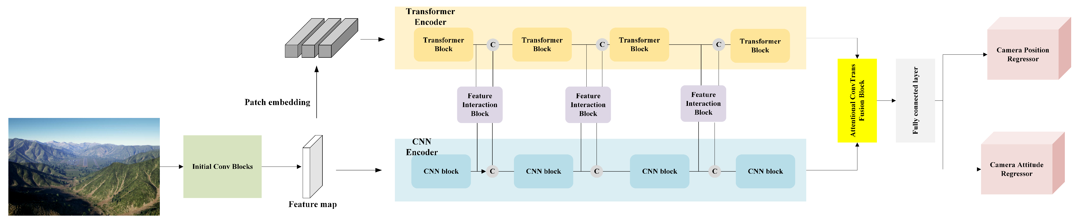
- We propose LandNet, a novel hybrid architecture combining Vision Transformer (ViT) and Convolutional Neural Networks (CNN) for 6-DoF camera relocalization using single images. LandNet is designed to efficiently generalize to large-scale environments, providing robustness for fixed-wing aircraft landing applications.
- We propose a Feature Interaction Block that fully leverages both spatial and temporal information to enhance image representations for absolute pose regression.
- An Attentional ConvTrans Fusion Block is designed to effectively integrate multi-scale and multi-level information to improve camera prediction.
- We evaluate the proposed LandNet using real flight data. The experimental results show that the method performs effectively in fixed-wing aircraft landing scenarios, especially in terms of the accuracy of the predicted orientation.
2. Preliminary Knowledge
2.1. Attitude Transformation
2.1.1. From Quaternion to Euler Angle
2.1.2. From Euler Angle to Quaternion
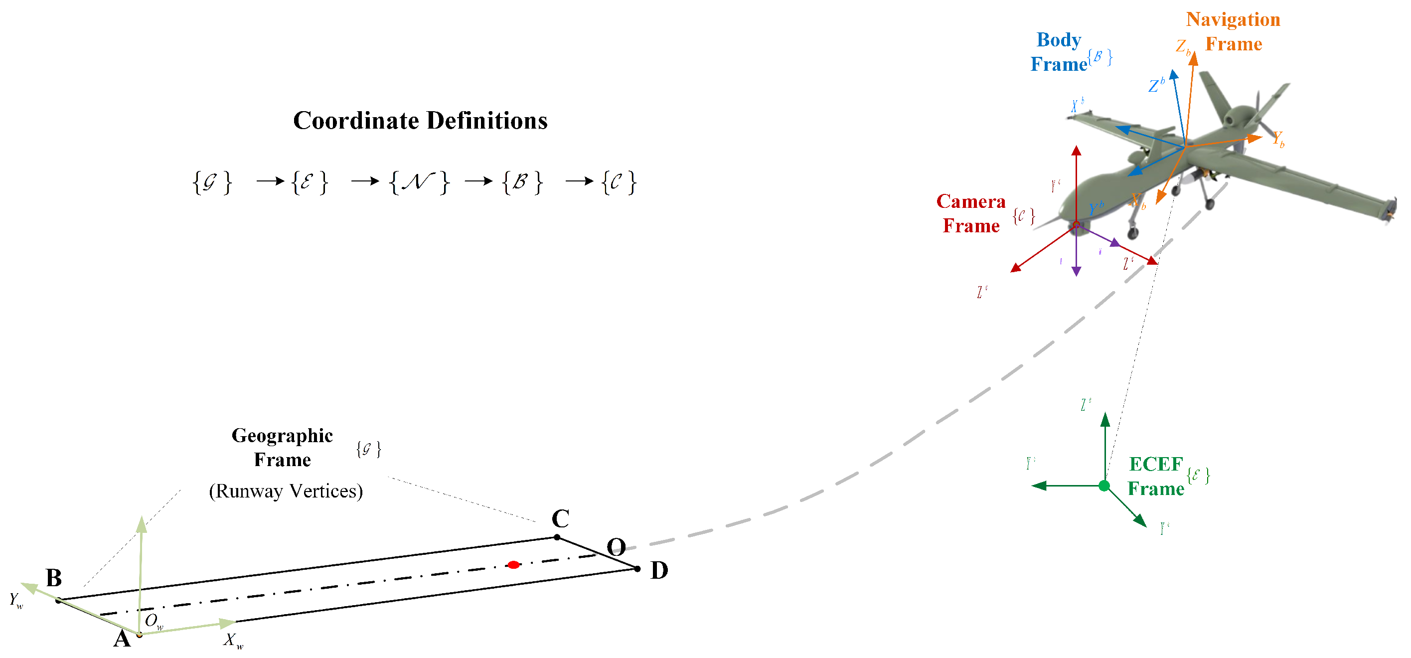
2.2. Coordinates Definitions
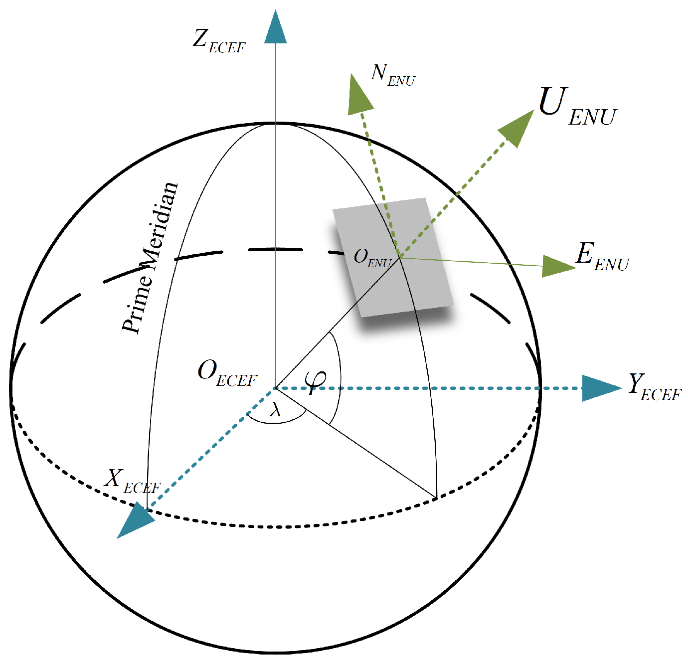
2.2.1. WGS84 to ECEF
2.2.2. ECEF to ENU
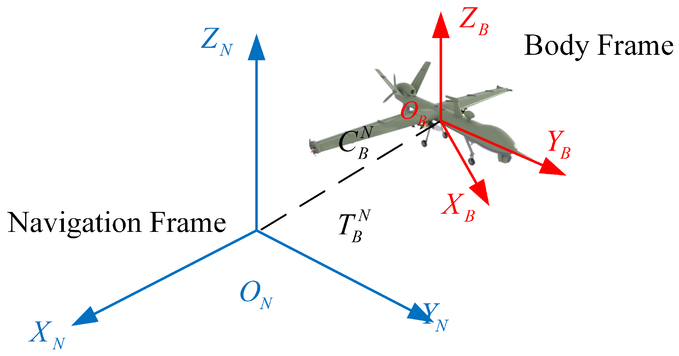
2.2.3. ENU to Body
2.2.4. Body to Camera
2.2.5. World Coordinate
2.3. Procedure for the Fixed-Wing Aircraft Landing
3. Methodology
3.1. Network Architecture
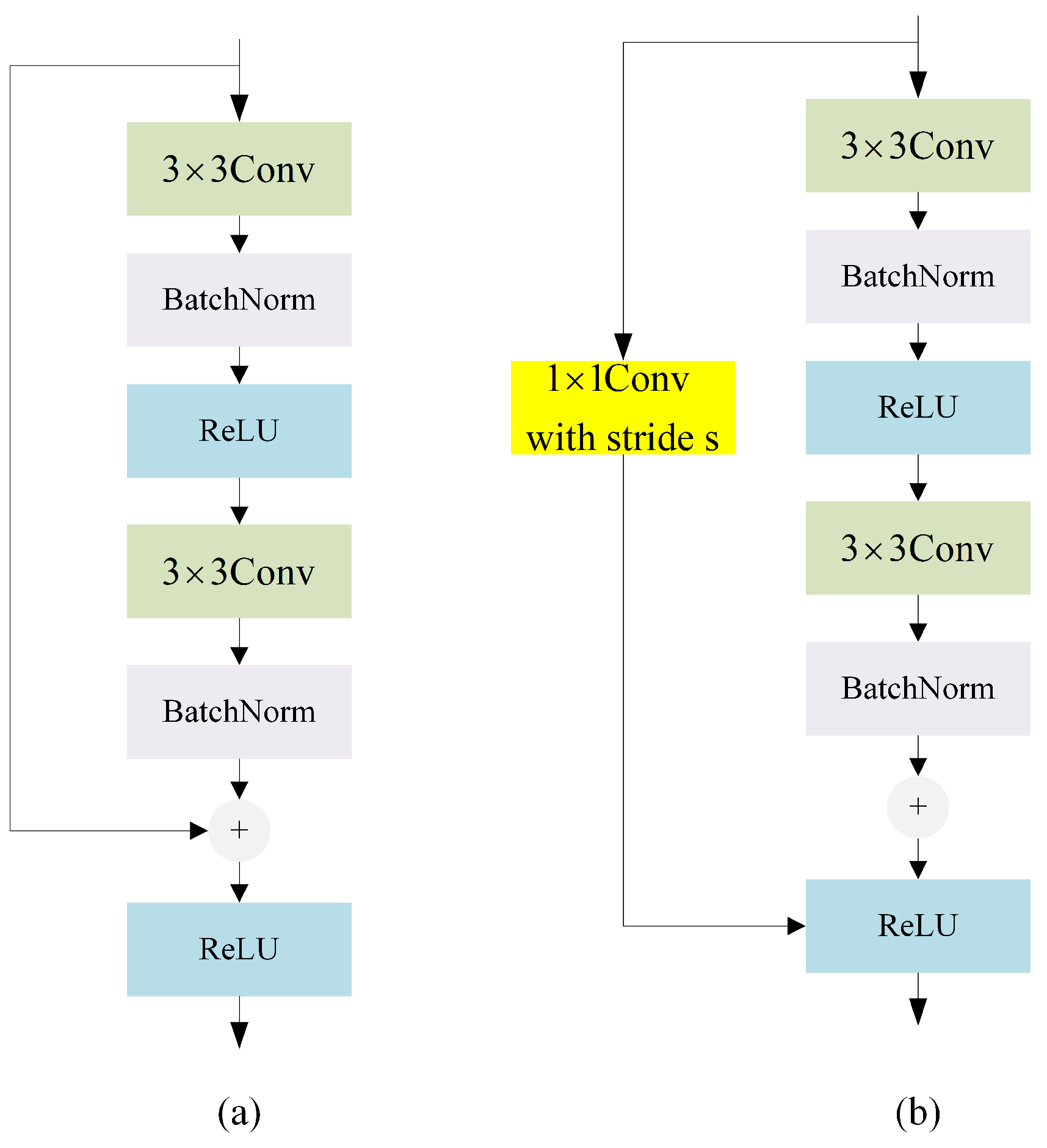
3.2. Initial Convolutional Blocks
3.3. CNN Encoder
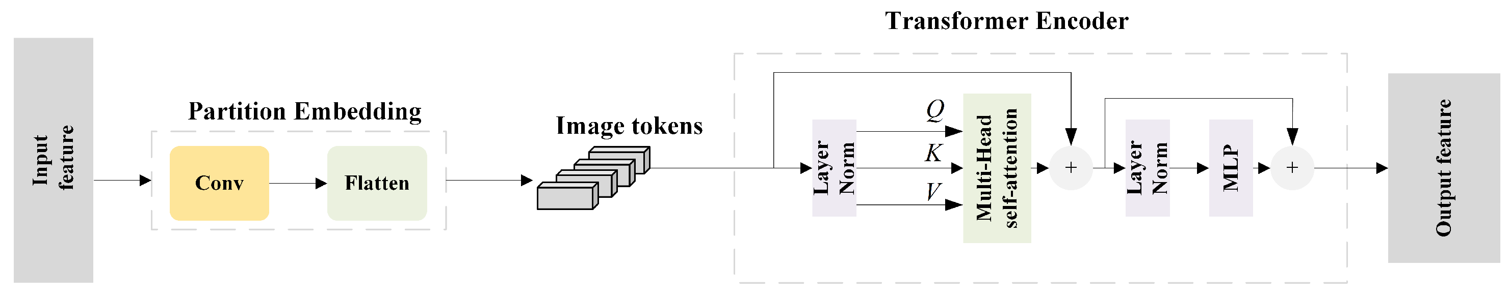
3.4. Transformer Encoder
3.5. Feature Interactive Block
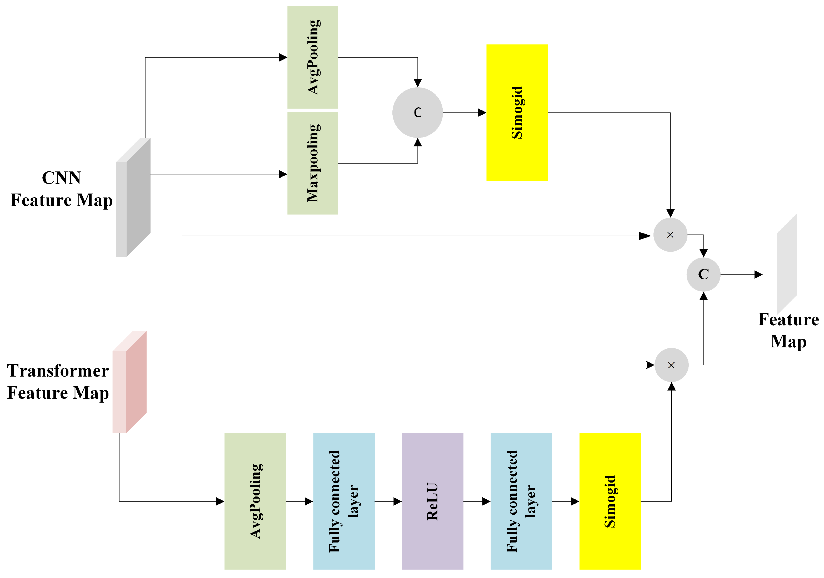
3.6. Attentional ConvTrans Fusion Block
3.7. Loss Function Design
4. Experiments
4.1. Datasets
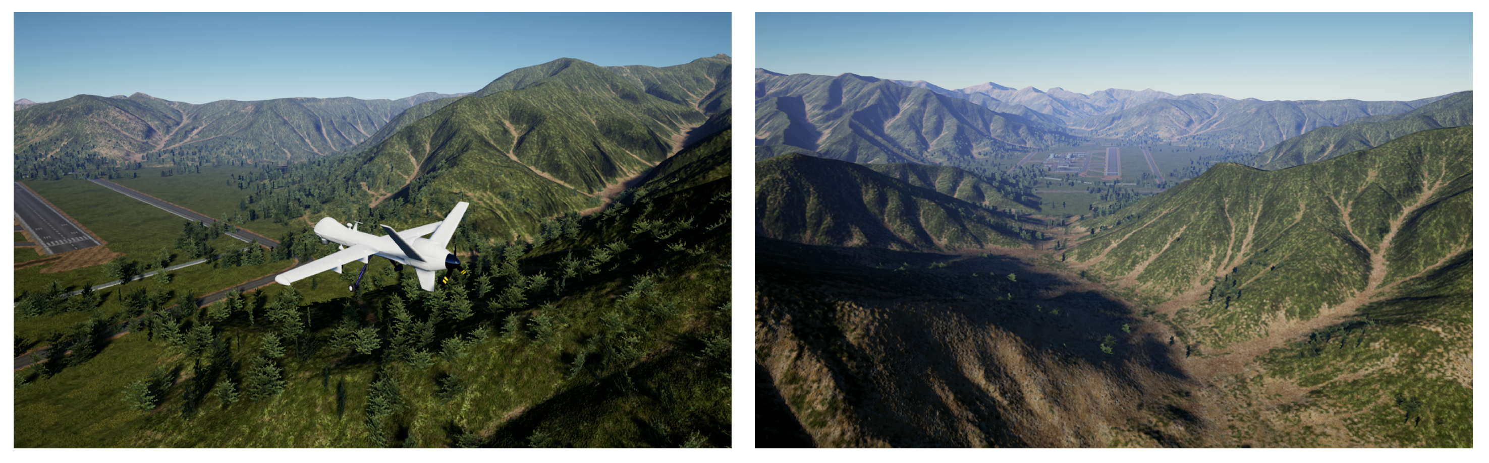
4.1.1. Simulation Data
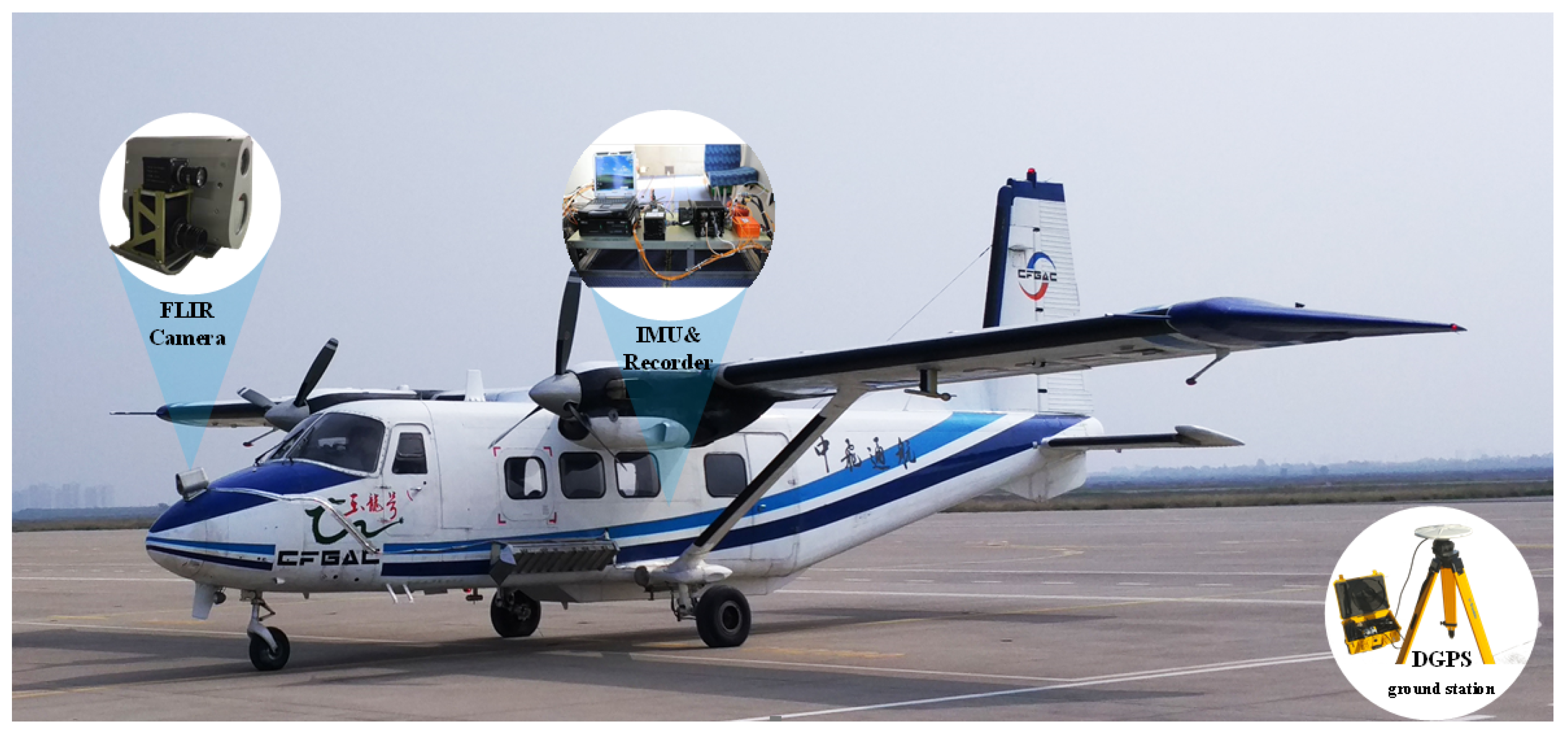
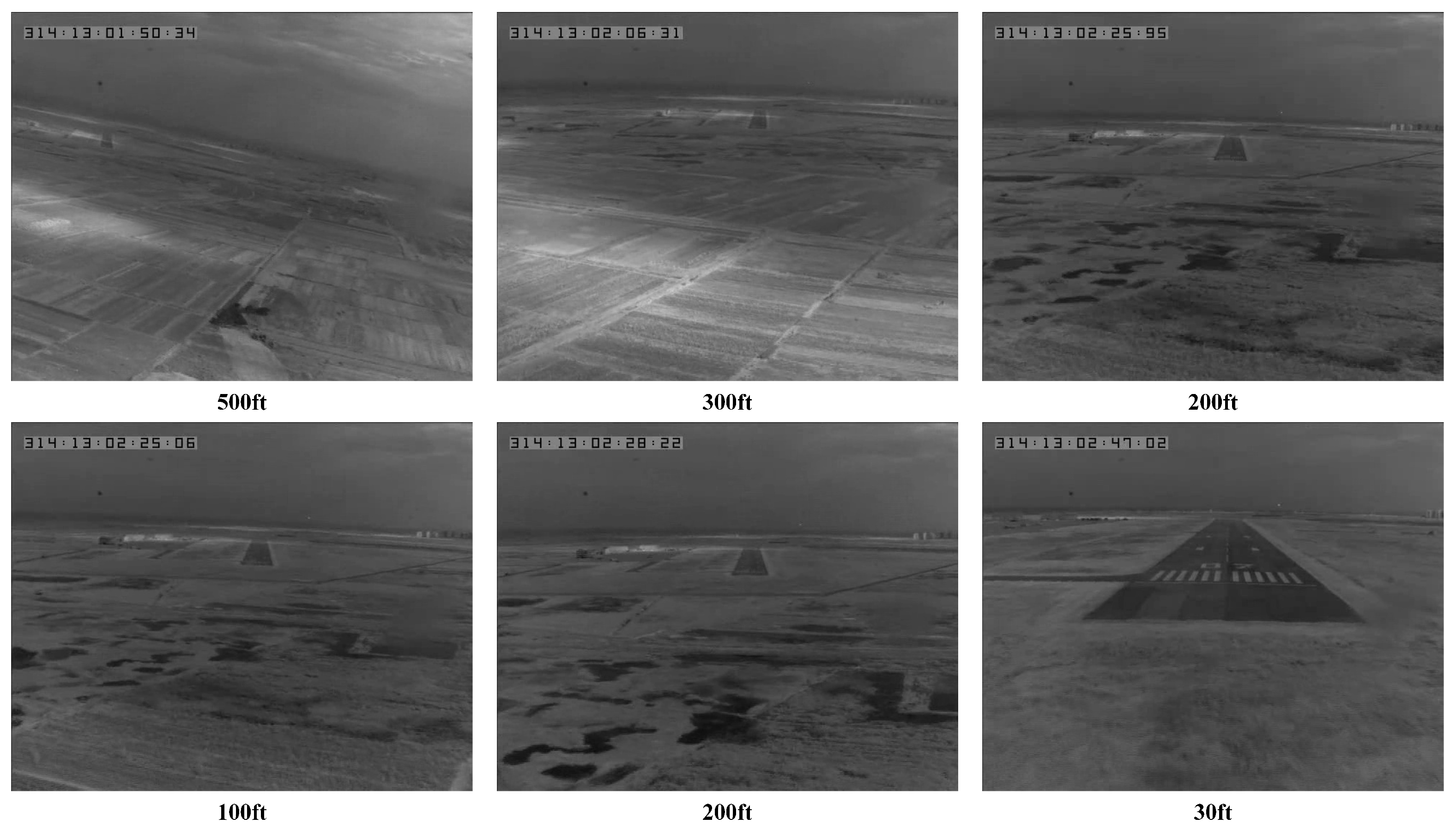
4.1.2. Flight Data Acquisition
4.2. Data Preparation
Data Processing
4.3. Training Details
4.4. Testing Metric Definitions
4.5. Experimental Results
4.5.1. Simulation Results
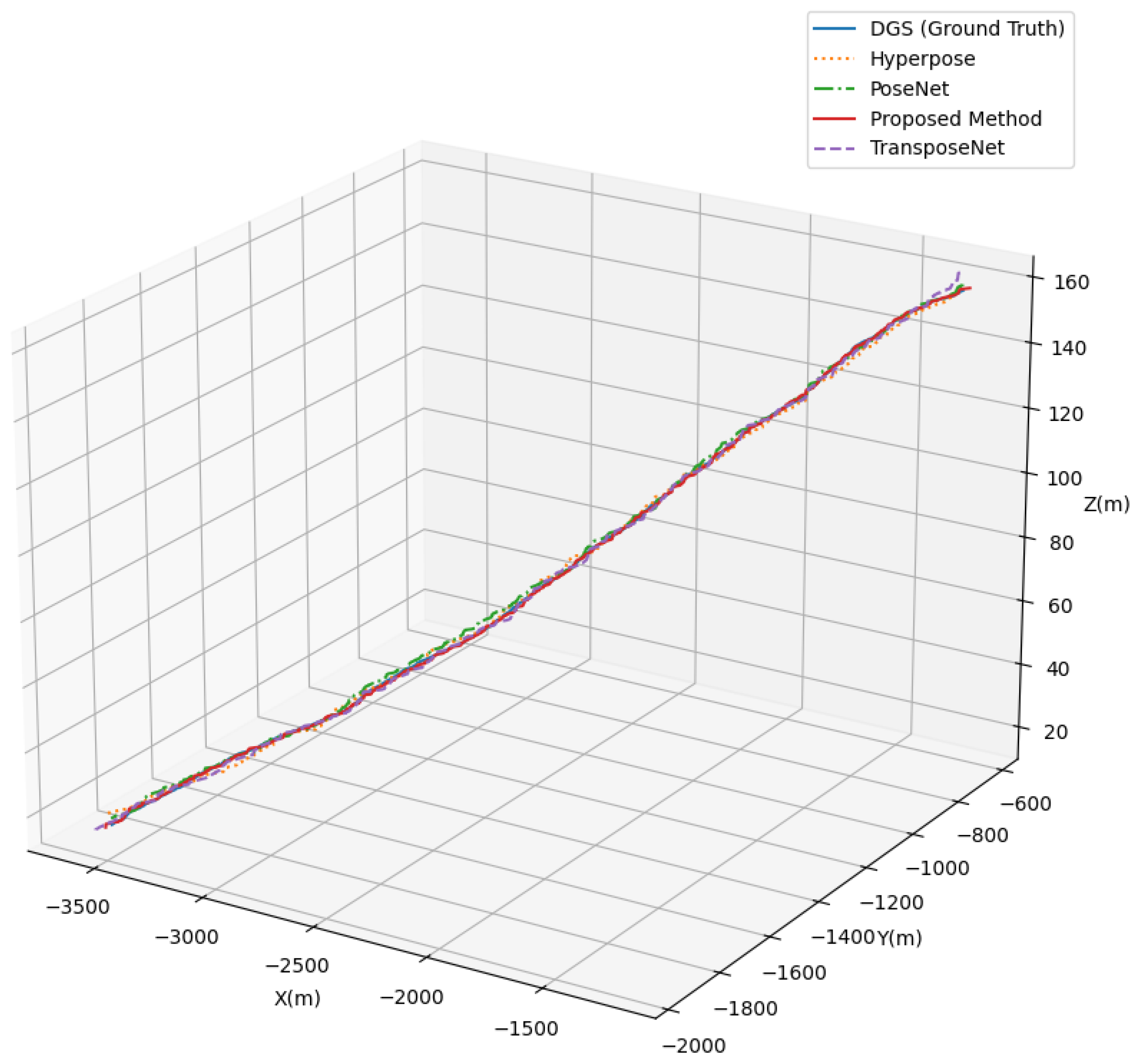
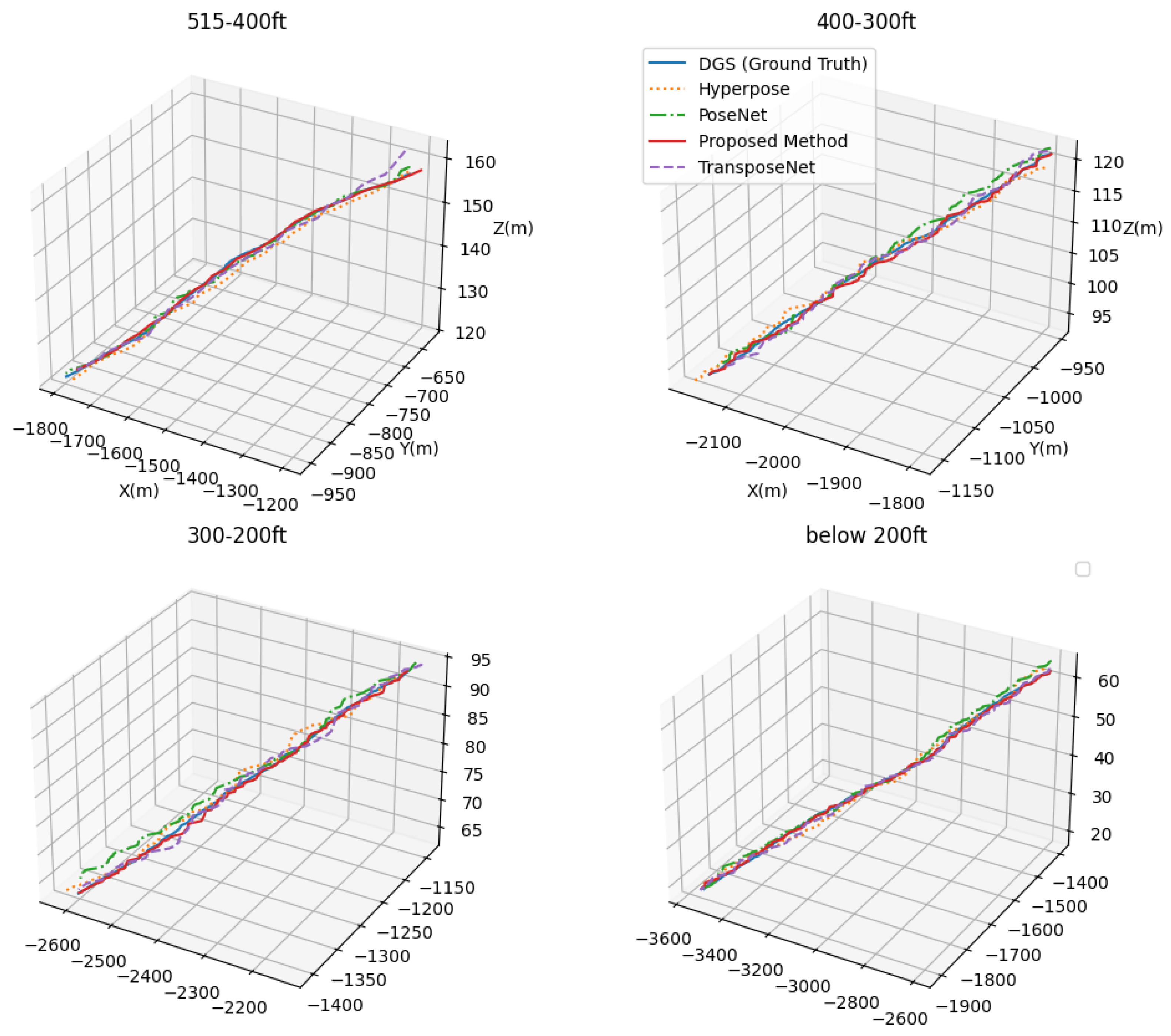
4.5.2. Results on Real-Flight Data
4.6. Ablation Study
4.6.1. Ablation on Parameter Inside CNN and the Transformer
4.6.2. Abaltion Study on FIB and ACFB Module
4.6.3. Sensitivity Study for and
5. Conclusions
Author Contributions
Funding
Data Availability Statement
Conflicts of Interest
Abbreviations
| 6DoF | Six-Degrees of Freedom |
| GNSS | Global Navigation Satellite System |
| INS | Inertial Navigation System |
| UAV | Unmanned Aerial Vehicle |
| DSO | Direct Sparse Odometry |
| VO | Visual Odometry |
| ECEF | Earth-Centered, Earth-Fixed frame |
| DA | Decision Altitude |
| CNNs | Convolutional Neural Networks |
References
- Zhang, Z.; Song, Y.; Huang, S.; Xiong, R.; Wang, Y. Toward consistent and efficient map-based visual-inertial localization: Theory framework and filter design. IEEE Trans. Robot. 2023, 39, 2892–2911. [Google Scholar] [CrossRef]
- Gallo, E.; Barrientos, A. Long-Distance GNSS-Denied Visual Inertial Navigation for Autonomous Fixed-Wing Unmanned Air Vehicles: SO (3) Manifold Filter Based on Virtual Vision Sensor. Aerospace 2023, 10, 708. [Google Scholar] [CrossRef]
- Lee, K.; Johnson, E.N. Latency compensated visual-inertial odometry for agile autonomous flight. Sensors 2020, 20, 2209. [Google Scholar] [CrossRef] [PubMed]
- Song, X.; Zhang, L.; Zhai, Z.; Yu, G. A Multimode Visual-Inertial Navigation Method for Fixed-wing Aircraft Approach and Landing in GPS-denied and Low Visibility Environments. In Proceedings of the 2019 IEEE/AIAA 38th Digital Avionics Systems Conference (DASC), San Diego, CA, USA, 8–12 September 2019; pp. 1–10. [Google Scholar]
- Van Der Merwe, R.; Wan, E.A. The square-root unscented Kalman filter for state and parameter-estimation. In Proceedings of the 2001 IEEE International Conference on Acoustics, Speech, and Signal Processing. Proceedings (Cat. No. 01CH37221), Salt Lake City, UT, USA, 7–11 May 2001; Volume 6, pp. 3461–3464. [Google Scholar]
- Engel, J.; Koltun, V.; Cremers, D. Direct sparse odometry. IEEE Trans. Pattern Anal. Mach. Intell. 2017, 40, 611–625. [Google Scholar] [CrossRef] [PubMed]
- Ellingson, G.; Brink, K.; McLain, T. Relative navigation of fixed-wing aircraft in GPS-denied environments. NAVIGATION J. Inst. Navig. 2020, 67, 255–273. [Google Scholar] [CrossRef]
- Seiskari, O.; Rantalankila, P.; Kannala, J.; Ylilammi, J.; Rahtu, E.; Solin, A. HybVIO: Pushing the limits of real-time visual-inertial odometry. In Proceedings of the IEEE/CVF Winter Conference on Applications of Computer Vision, Waikoloa, HI, USA, 3–8 January 2022; pp. 701–710. [Google Scholar]
- Wang, Z.; Pang, B.; Song, Y.; Yuan, X.; Xu, Q.; Li, Y. Robust visual-inertial odometry based on a kalman filter and factor graph. IEEE Trans. Intell. Transp. Syst. 2023, 24, 7048–7060. [Google Scholar] [CrossRef]
- Guan, W.; Chen, P.; Xie, Y.; Lu, P. Pl-evio: Robust monocular event-based visual inertial odometry with point and line features. IEEE Trans. Autom. Sci. Eng. 2023, 21, 6277–6293. [Google Scholar] [CrossRef]
- Cao, S.; Lu, X.; Gvins, S.S. Tightly coupled GNSS-visual-inertial fusion for smooth and consistent state estimation. IEEE Trans. Robot. 2022, 38, 2004–2021. [Google Scholar] [CrossRef]
- Leutenegger, S. Okvis2: Realtime scalable visual-inertial slam with loop closure. arXiv 2022, arXiv:2202.09199. [Google Scholar]
- Liu, X.; Li, C.; Xu, X.; Yang, N.; Qin, B. Implicit Neural Mapping for a Data Closed-Loop Unmanned Aerial Vehicle Pose-Estimation Algorithm in a Vision-Only Landing System. Drones 2023, 7, 529. [Google Scholar] [CrossRef]
- Hou, B.; Ding, X.; Bu, Y.; Liu, C.; Shou, Y.; Xu, B. Visual Inertial Navigation Optimization Method Based on Landmark Recognition. In Proceedings of the International Conference on Cognitive Computation and Systems, Beijing, China, 17–18 December 2022; pp. 212–223. [Google Scholar]
- Huang, L.; Song, J.; Zhang, C. Observability analysis and filter design for a vision inertial absolute navigation system for UAV using landmarks. Optik 2017, 149, 455–468. [Google Scholar] [CrossRef]
- Wang, Z.; Zhao, D.; Cao, Y. Visual navigation algorithm for night landing of fixed-wing unmanned aerial vehicle. Aerospace 2022, 9, 615. [Google Scholar] [CrossRef]
- Girshick, R. Fast r-cnn. In Proceedings of the IEEE International Conference on Computer Vision, Santiago, Chile, 7–13 December 2015; pp. 1440–1448. [Google Scholar]
- Yu, G.; Zhang, L.; Zou, C.; Liu, Y.; Cheng, Y. A Robust and Real-time Visual-Inertial Pose Estimation for Fixed-wing Aircraft Landing. In Proceedings of the 32nd Congress of the International Council of the Aeronautical Sciences, Shanghai, China, 6–10 September 2021; pp. 4398–4409. [Google Scholar]
- Yu, G.; Zhang, L.; Shen, S.; Zhai, Z. Real-time vision-inertial landing navigation for fixed-wing aircraft with CFC-CKF. Complex Intell. Syst. 2024, 10, 8079–8093. [Google Scholar] [CrossRef]
- Dusha, D.; Mejias, L.; Walker, R. Fixed-wing attitude estimation using temporal tracking of the horizon and optical flow. J. Field Robot. 2011, 28, 355–372. [Google Scholar] [CrossRef]
- Grof, T.; Bauer, P.; Hiba, A.; Gati, A.; Zarándy, Á.; Vanek, B. Runway relative positioning of aircraft with IMU-camera data fusion. IFAC-PapersOnLine 2019, 52, 376–381. [Google Scholar] [CrossRef]
- Shang, K.; Li, X.; Liu, C.; Ming, L.; Hu, G. An Integrated Navigation Method for UAV Autonomous Landing Based on Inertial and Vision Sensors. In Proceedings of the CAAI International Conference on Artificial Intelligence, Beijing, China, 27–28 August 2022; pp. 182–193. [Google Scholar]
- Macario Barros, A.; Michel, M.; Moline, Y.; Corre, G.; Carrel, F. A comprehensive survey of visual slam algorithms. Robotics 2022, 11, 24. [Google Scholar] [CrossRef]
- Li, Q.; Cao, R.; Zhu, J.; Hou, X.; Liu, J.; Jia, S.; Li, Q.; Qiu, G. Improving synthetic 3D model-aided indoor image localization via domain adaptation. ISPRS J. Photogramm. Remote Sens. 2022, 183, 66–78. [Google Scholar] [CrossRef]
- Sattler, T.; Zhou, Q.; Pollefeys, M.; Leal-Taixe, L. Understanding the limitations of cnn-based absolute camera pose regression. In Proceedings of the IEEE/CVF Conference on Computer Vision and Pattern Recognition, Long Beach, CA, USA, 15–20 June 2019; pp. 3302–3312. [Google Scholar]
- Zhuang, S.; Zhao, Z.; Cao, L.; Wang, D.; Fu, C.; Du, K. A robust and fast method to the perspective-n-point problem for camera pose estimation. IEEE Sens. J. 2023, 23, 11892–11906. [Google Scholar] [CrossRef]
- Kendall, A.; Grimes, M.; Cipolla, R. Posenet: A convolutional network for real-time 6-dof camera relocalization. In Proceedings of the IEEE International Conference on Computer Vision, Santiago, Chile, 7–13 December 2015; pp. 2938–2946. [Google Scholar]
- Liu, K.; Li, Q.; Qiu, G. PoseGAN: A pose-to-image translation framework for camera localization. ISPRS J. Photogramm. Remote Sens. 2020, 166, 308–315. [Google Scholar] [CrossRef]
- Shavit, Y.; Ferens, R.; Keller, Y. Coarse-to-fine multi-scene pose regression with transformers. IEEE Trans. Pattern Anal. Mach. Intell. 2023, 45, 14222–14233. [Google Scholar] [CrossRef]
- Brahmbhatt, S.; Gu, J.; Kim, K.; Hays, J.; Kautz, J. Geometry-aware learning of maps for camera localization. In Proceedings of the IEEE Conference on Computer Vision and Pattern Recognition, Salt Lake City, UT, USA, 18–23 June 2018; pp. 2616–2625. [Google Scholar]
- Gao, H.; Dai, K.; Wang, K.; Li, R.; Zhao, L.; Wu, M. ALNet: An adaptive channel attention network with local discrepancy perception for accurate indoor visual localization. Expert Syst. Appl. 2024, 250, 123792. [Google Scholar] [CrossRef]
- Wang, J.; Zhou, K.; Markham, A.; Trigoni, N. MambaLoc: Efficient Camera Localisation via State Space Model. arXiv 2024, arXiv:2408.09680. [Google Scholar]
- Yang, C.; Liu, Y.; Zell, A. RCPNet: Deep-learning based relative camera pose estimation for UAVs. In Proceedings of the 2020 International Conference on Unmanned Aircraft Systems (ICUAS), Athens, Greece, 1–4 September 2020; pp. 1085–1092. [Google Scholar]
- Baldini, F.; Anandkumar, A.; Murray, R.M. Learning pose estimation for UAV autonomous navigation and landing using visual-inertial sensor data. In Proceedings of the 2020 American Control Conference (ACC), Denver, CO, USA, 1–3 July 2020; pp. 2961–2966. [Google Scholar]
- Shan, P.; Yang, R.; Xiao, H.; Zhang, L.; Liu, Y.; Fu, Q.; Zhao, Y. UAVPNet: A balanced and enhanced UAV object detection and pose recognition network. Measurement 2023, 222, 113654. [Google Scholar] [CrossRef]
- Lowe, D.G. Distinctive image features from scale-invariant keypoints. Int. J. Comput. Vis. 2004, 60, 91–110. [Google Scholar] [CrossRef]
- Vaswani, A.; Shazeer, N.; Parmar, N.; Uszkoreit, J.; Jones, L.; Gomez, A.N.; Kaiser, L.; Polosukhin, I. Attention is all you need. Adv. Neural. Inf. Process. Syst. 2017, 5998–6008. [Google Scholar]
- He, K.; Zhang, X.; Ren, S.; Sun, J. Deep residual learning for image recognition. In Proceedings of the IEEE Conference on Computer Vision and Pattern Recognition, Las Vegas, NV, USA, 27–30 June 2016; pp. 770–778. [Google Scholar]
- Dosovitskiy, A.; Beyer, L.; Kolesnikov, A.; Weissenborn, D.; Zhai, X.; Unterthiner, T.; Dehghani, M.; Minderer, M.; Heigold, G.; Gelly, S. An image is worth 16x16 words: Transformers for image recognition at scale. arXiv 2020, arXiv:2010.11929. [Google Scholar]
- Geng, P.; Lu, J.; Zhang, Y.; Ma, S.; Tang, Z.; Liu, J. TC-Fuse: A Transformers Fusing CNNs Network for Medical Image Segmentation. CMES-Comput. Model. Eng. Sci. 2023, 137, 2001–2023. [Google Scholar] [CrossRef]
- Hu, J.; Shen, L.; Sun, G. Squeeze-and-excitation networks. In Proceedings of the IEEE Conference on Computer Vision and Pattern Recognition, Salt Lake City, UT, USA, 18–23 June 2018; pp. 7132–7141. [Google Scholar]
- Paszke, A.; Gross, S.; Massa, F.; Lerer, A.; Bradbury, J.; Chanan, G.; Killeen, T.; Lin, Z.; Gimelshein, N.; Antiga, L. Pytorch: An imperative style, high-performance deep learning library. Adv. Neural. Inf. Process. Syst. 2019, 32, 721. [Google Scholar]
- Shavit, Y.; Ferens, R. Do we really need scene-specific pose encoders? In Proceedings of the 2020 25th International Conference on Pattern Recognition (ICPR), Milan, Italy, 10–15 January 2021; pp. 3186–3192. [Google Scholar]
- Wang, B.; Chen, C.; Lu, C.X.; Zhao, P.; Trigoni, N.; Markham, A. Atloc: Attention guided camera localization. In Proceedings of the AAAI Conference on Artificial Intelligence, New York, NY, USA, 7–12 February 2020; Volume 34, pp. 10393–10401. [Google Scholar]
- Ferens, R.; Keller, Y. Hyperpose: Camera pose localization using attention hypernetworks. arXiv 2023, arXiv:2303.02610. [Google Scholar]
- Shavit, Y.; Ferens, R.; Keller, Y. Paying attention to activation maps in camera pose regression. arXiv 2021, arXiv:2103.11477. [Google Scholar]
- Leng, K.; Yang, C.; Sui, W.; Liu, J.; Li, Z. Sitpose: A Siamese Convolutional Transformer for Relative Camera Pose Estimation. In Proceedings of the 2023 IEEE International Conference on Multimedia and Expo (ICME), Brisbane, Australia, 10–14 July 2023; pp. 1871–1876. [Google Scholar]
- Shavit, Y.; Ferens, R.; Keller, Y. Learning single and multi-scene camera pose regression with transformer encoders. Comput. Vis. Image Underst. 2024, 243, 103982. [Google Scholar] [CrossRef]


| Stage | Kernel Size × Channels | Repeated Times |
|---|---|---|
| 1 | ||
| 3 | ||
| 4 | ||
| 3 | ||
| 1 | ||
| Parameters Type | Specific Parameters | Values |
|---|---|---|
| Camera intrinsic parameters | Pixel size | m |
| Resolution | 640 × 512 | |
| Focal length | ||
| Radial distortion | ||
| IMU installation on the aircraft | Position | m |
| Camera installation | Attitude | |
| Position | m |
| Method | (m) | (m) | (m) | (deg) | (deg) | (deg) |
|---|---|---|---|---|---|---|
| PoseNet [27] | 13.9 | 9.2 | 1.3 | 0.235 | 0.381 | 0.328 |
| IRPNet [43] | 11.1 | 10.2 | 1.5 | 0.286 | 0.394 | 0.271 |
| Atlocc [44] | 10.8 | 8.5 | 1.4 | 0.301 | 0.372 | 0.249 |
| HyperPoseNet [45] | 8.9 | 9.1 | 1.19 | 0.201 | 0.453 | 0.232 |
| TransPose [46] | 8.4 | 8.7 | 1.26 | 0.257 | 0.371 | 0.295 |
| LandNet | 7.6 | 7.3 | 0.9 | 0.110 | 0.339 | 0.218 |
| Flight Height (ft) | Category | Methods | (m) | (m) | (m) | (deg) | (deg) | (deg) |
|---|---|---|---|---|---|---|---|---|
| 515–400 | CNN-based | PoseNet [27] | 12.5 | 5.7 | 0.9 | 0.070 | 0.080 | 0.020 |
| IRPNet [43] | 12.3 | 10.5 | 1.9 | 0.018 | 0.009 | 0.038 | ||
| Atloc [44] | 9.5 | 7.9 | 1.1 | 0.010 | 0.033 | 0.025 | ||
| HyperPoseNet [45] | 9.2 | 5.8 | 1.8 | 0.020 | 0.010 | 0.030 | ||
| Transformer-based | SitPose [47] | 12.8 | 35.7 | 3.34 | 0.058 | 0.060 | 0.203 | |
| TransPose [46] | 9.4 | 8.7 | 1.6 | 0.053 | 0.048 | 0.051 | ||
| TransencoderNet [48] | 8.3 | 9.3 | 1.1 | 0.045 | 0.034 | 0.029 | ||
| LandNet | 6.2 | 3.5 | 0.2 | 0.020 | 0.010 | 0.030 | ||
| 400–300 | CNN-based | PoseNet [27] | 6.5 | 3.9 | 1.1 | 0.002 | 0.020 | 0.050 |
| IRPNet [43] | 13.6 | 6.4 | 0.9 | 0.021 | 0.004 | 0.029 | ||
| Atloc [44] | 7.5 | 5.2 | 2.6 | 0.004 | 0.006 | 0.008 | ||
| HyperPoseNet [45] | 11.1 | 5.9 | 1.2 | 0.006 | 0.003 | 0.008 | ||
| Transformer-based | SitPose [47] | 10.0 | 7.5 | 0.4 | 0.009 | 0.033 | 0.104 | |
| TransPose [46] | 9.3 | 5.5 | 1.2 | 0.036 | 0.048 | 0.029 | ||
| TransencoderNet [48] | 8.8 | 6.6 | 0.9 | 0.032 | 0.031 | 0.032 | ||
| LandNet | 7.0 | 3.7 | 0.7 | 0.003 | 0.002 | 0.007 | ||
| 300–200 | CNN-based | PoseNet [27] | 9.2 | 4.4 | 1.9 | 0.003 | 0.020 | 0.003 |
| IRPNet [43] | 22.2 | 10.6 | 0.88 | 0.016 | 0.001 | 0.014 | ||
| Atloc [44] | 11.8 | 7.2 | 2.5 | 0.004 | 0.001 | 0.006 | ||
| HyperPoseNet [45] | 7.3 | 3.8 | 1.7 | 0.006 | 0.004 | 0.040 | ||
| Transformer-based | SitPose [47] | 13.5 | 8.5 | 1.1 | 0.025 | 0.016 | 0.073 | |
| TransPose [46] | 9.5 | 5.3 | 1.3 | 0.021 | 0.030 | 0.015 | ||
| TransencoderNet [48] | 8.3 | 5.6 | 0.9 | 0.022 | 0.027 | 0.019 | ||
| LandNet | 7.5 | 2.8 | 0.9 | 0.003 | 0.001 | 0.006 | ||
| Below 200 | CNN-based | PoseNet [27] | 14.5 | 6.0 | 1.4 | 0.015 | 0.017 | 0.030 |
| IRPNet [43] | 9.2 | 5.8 | 1.8 | 0.021 | 0.007 | 0.033 | ||
| Atloc [44] | 5.1 | 4.9 | 1.8 | 0.005 | 0.001 | 0.009 | ||
| HyperPoseNet [45] | 15.0 | 3.9 | 2.2 | 0.017 | 0.002 | 0.030 | ||
| Transformer-based | SitPose [47] | 12.5 | 11.4 | 1.2 | 0.015 | 0.003 | 0.015 | |
| TransPose [46] | 9.3 | 6.0 | 1.1 | 0.021 | 0.033 | 0.018 | ||
| TransencoderNet [48] | 6.3 | 7.3 | 0.8 | 0.020 | 0.019 | 0.021 | ||
| LandNet | 4.9 | 6.5 | 0.9 | 0.016 | 0.002 | 0.001 |
| Transformer Branch | CNN Branch | (m) | (m) | (m) | (deg) | (deg) | (deg) | |
|---|---|---|---|---|---|---|---|---|
| Embedding Dimension | Heads | Channel | ||||||
| 384 | 6 | 64 | 12.34 | 9.12 | 1.91 | 0.035 | 0.025 | 0.063 |
| 128 | 11.08 | 8.52 | 1.58 | 0.032 | 0.016 | 0.040 | ||
| 512 | 10.98 | 7.92 | 1.12 | 0.026 | 0.013 | 0.032 | ||
| 576 | 9 | 256 | 10.65 | 8.31 | 1.56 | 0.023 | 0.011 | 0.036 |
| 768 | 12 | 256 | 9.34 | 6.07 | 0.93 | 0.020 | 0.005 | 0.031 |
| Module | (m) | (m) | (m) | (deg) | (deg) | (deg) | |
|---|---|---|---|---|---|---|---|
| FIB | ACFB | ||||||
| ✓ | ✓ | 9.34 | 6.07 | 0.93 | 0.020 | 0.005 | 0.031 |
| ✓ | 10.45 | 6.78 | 1.22 | 0.026 | 0.006 | 0.030 | |
| ✓ | 9.56 | 7.12 | 1.32 | 0.030 | 0.011 | 0.038 | |
| (m) | (m) | (m) | (deg) | (deg) | (deg) | ||
|---|---|---|---|---|---|---|---|
| 3 | 0 | 9.34 | 6.07 | 0.93 | 0.020 | 0.005 | 0.031 |
| 0 | 0 | 14.93 | 7.74 | 1.29 | 0.024 | 0.006 | 0.033 |
| 0 | 2 | 12.20 | 7.62 | 0.91 | 0.022 | 0.006 | 0.03 |
Disclaimer/Publisher’s Note: The statements, opinions and data contained in all publications are solely those of the individual author(s) and contributor(s) and not of MDPI and/or the editor(s). MDPI and/or the editor(s) disclaim responsibility for any injury to people or property resulting from any ideas, methods, instructions or products referred to in the content. |
© 2025 by the authors. Licensee MDPI, Basel, Switzerland. This article is an open access article distributed under the terms and conditions of the Creative Commons Attribution (CC BY) license (https://creativecommons.org/licenses/by/4.0/).
Share and Cite
Shen, S.; Yu, G.; Zhang, L.; Yan, Y.; Zhai, Z. LandNet: Combine CNN and Transformer to Learn Absolute Camera Pose for the Fixed-Wing Aircraft Approach and Landing. Remote Sens. 2025, 17, 653. https://doi.org/10.3390/rs17040653
Shen S, Yu G, Zhang L, Yan Y, Zhai Z. LandNet: Combine CNN and Transformer to Learn Absolute Camera Pose for the Fixed-Wing Aircraft Approach and Landing. Remote Sensing. 2025; 17(4):653. https://doi.org/10.3390/rs17040653
Chicago/Turabian StyleShen, Siyuan, Guanfeng Yu, Lei Zhang, Youyu Yan, and Zhengjun Zhai. 2025. "LandNet: Combine CNN and Transformer to Learn Absolute Camera Pose for the Fixed-Wing Aircraft Approach and Landing" Remote Sensing 17, no. 4: 653. https://doi.org/10.3390/rs17040653
APA StyleShen, S., Yu, G., Zhang, L., Yan, Y., & Zhai, Z. (2025). LandNet: Combine CNN and Transformer to Learn Absolute Camera Pose for the Fixed-Wing Aircraft Approach and Landing. Remote Sensing, 17(4), 653. https://doi.org/10.3390/rs17040653