Deep Learning-Based Feature Matching Algorithm for Multi-Beam and Side-Scan Images

Abstract

Side-scan sonar and multi-beam echo sounder (MBES) are the most widely used underwater surveying tools in marine mapping today. The MBES offers high accuracy in depth measurement but is limited by low imaging resolution due to beam density constraints. Conversely, side-scan sonar provides high-resolution backscatter intensity images but lacks precise positional information and often suffers from distortions. Thus, MBES and side-scan images complement each other in depth accuracy and imaging resolution. To obtain high-quality seafloor topography images in practice, matching between MBES and side-scan images is necessary. However, due to the significant differences in content and resolution between MBES depth images and side-scan backscatter images, they represent a typical example of heterogeneous images, making feature matching difficult with traditional image matching methods. To address this issue, this paper proposes a feature matching network based on the LoFTR algorithm, utilizing the intermediate layers of the ResNet-50 network to extract shared features between the two types of images. By leveraging self-attention and cross-attention mechanisms, the features of the MBES and side-scan images are combined, and a similarity matrix of the two modalities is calculated to achieve mutual matching. Experimental results show that, compared to traditional methods, the proposed model exhibits greater robustness to noise interference and effectively reduces noise. It also overcomes challenges, such as large nonlinear differences, significant geometric distortions, and high matching difficulty between the MBES and side-scan images, significantly improving the optimized image matching results. The matching error RMSE has been reduced to within six pixels, enabling the accurate matching of multi-beam and side-scan images.

1. Introduction

Precisely detecting and identifying targets distributed on or buried within the seafloor, such as marine organisms, mineral resources, and underwater cultural heritage sites, is crucial for promoting the efficient development of marine resources, mineral and oil resources, as well as for the preservation of underwater cultural heritage [1,2,3]. The Multi-Beam Echo Sounder (MBES) achieves high-precision underwater topographic mapping by emitting directional beams, intensively sampling echo signals, and measuring the phase of return signals, which allows for calculating the depth and generating full-coverage 3D bathymetric images over large areas [4,5,6]. The Side-Scan Sonar (SSS), usually mounted on a towed fish and deployed from survey vessels, emits wide-angle beams on both sides, recording the intensity of echo signals based on the time they reach the transducers, to create high-resolution underwater topographic images [7]. In practice, MBES is often used for precise depth measurement applications, such as seabed mapping and engineering construction [8], while SSS is applied for seabed target detection and large-area search, such as shipwreck surveys [2]. In real-world underwater topography surveys, these two sonar systems are frequently used together; MBES conducts an initial broad sweep to locate targets, followed by SSS for detailed mapping and analysis.

The MBES achieves high-accuracy underwater positioning information by precisely measuring the round-trip time and arrival angles of acoustic waves, allowing it to capture detailed underwater topographic images and backscatter intensity maps. Its beamforming is achieved by using multiple receiving beams that cross-detect the seabed, allowing for segmented signal processing to obtain measurement data from different angles. However, the beamforming method of the side-scan sonar involves receiving time-sequenced echo signals reflected from the seabed during lateral scanning, allowing for a wider scanning range. Side-scan sonar typically has a smaller pitch angle, especially when close to the seabed, providing higher image resolution and thus, enabling the generation of high-resolution backscatter intensity images of the seafloor [9]. To improve detection resolution and reduce the impact of the vessel’s attitude, side-scan sonar is typically installed in a towed configuration. Factors, such as cable swinging, vessel speed, and uncertainties in the tow cable length, can cause the towed sonar device to drift, leading to a lack of accurate positional information in the observations. This affects the geographic accuracy of the measurement points and impacts both the imaging resolution and coverage area [10,11,12,13]. MBES provides precise depth data, while SSS supplies high-resolution, broad-range backscatter images. Therefore, matching high-resolution SSS backscatter images with accurately measured MBES depth images can enrich and enhance the information and detail of a single-source image, enabling the use of MBES location information to correct geographical distortions in SSS images and thus, accurately reflect the distribution and characteristics of the seafloor and target objects [14]. In addition, image matching, as a critical preliminary task, lays the foundation for the subsequent fusion of multi-beam and side-scan sonar images. By utilizing deep feature fusion techniques, it enables the generation of fused multi-beam and side-scan sonar images that combine high spatial accuracy with rich detail representation. This approach helps to overcome the limitations of single-sensor imaging and serves as a reliable basis for higher-level underwater detection tasks [15].

The MBES depth images and SSS backscatter images represent a typical case of heterogeneous images. Each pixel in MBES depth images corresponds to depth data [4], indicating the vertical distance from the seabed beam footprints to the depth reference plane and reflecting the seabed topography. In contrast, each pixel in SSS images represents echo intensity, which mainly depicts seabed surface textures and reflectivity characteristics [16,17]. Additionally, MBES and SSS images differ significantly in resolution. The lack of heading measurements and the low positional accuracy of the towed SSS system lead to substantial geometric distortions in SSS images. These factors increase the complexity of matching, making accurate alignment and fusion more challenging [18,19,20].

At present, image registration methods typically employ two approaches: traditional intensity-based registration and feature-based registration. Intensity-based methods do not require feature extraction and are straightforward to implement, but they perform poorly for heavily distorted images, especially heterogeneous images. Feature-based methods are more robust and suited for complex transformations, relying heavily on the selection of feature spaces and the extraction of feature points, thus, often underperforming on lower-resolution MBES images [21].

For the registration of MBES depth images and SSS backscatter images, due to the differences in imaging principles and the complexity of the marine environment, using intensity-based features for registration is challenging. Therefore, researchers primarily utilize feature-based image registration methods [22]. Yang Fanlin et al. combined MBES contour maps with SSS backscatter intensity data, extracting feature points from contours and depth lines, and achieved registration using MBES data as a reference [6]. Zhang Ning et al. proposed an iterative adaptive registration method, using wavelet transformation to extract low-frequency SSS image information for coarse registration with MBES images, followed by Demons algorithm for fine registration. However, they did not consider resolution differences, resulting in detail loss and lower fusion quality [23]. Shang Xiaodong and Zhao Jianhu applied the SURF algorithm with geographic coordinates as constraints to achieve coarse matching, then segmented SSS images, creating a geometric model for each segment to achieve automatic registration [24]. Wynn W M used the Chamfer algorithm for MBES and SSS automatic registration [25]. While these methods successfully achieved registration, they face challenges, such as high requirements for feature point selection, simplistic image transformations, and the inadequate handling of image detail differences [25]. These studies mainly rely on traditional registration methods, requiring numerous manual constraints (e.g., edge features), leading to limited robustness in handling heterogeneous images, especially MBES and SSS images with significant modal differences, and preventing effective feature extraction in complex underwater scenarios.

With the rapid development of deep learning, many image registration methods based on deep learning have been developed, constructing convolutional neural networks to learn descriptors, and addressing issues in traditional methods, such as high time costs and low robustness. Although deep learning-based feature matching algorithms have addressed some challenges in local feature extraction from acoustic images, the scarcity of acoustic trained datasets, and the limitations of convolutional neural networks (CNNs) [26], due to the limitations of the local receptive field, CNNs face difficulties when processing images with significant modal differences. The features detected by the algorithm tend to concentrate on corners and edges, making it challenging to detect features in areas with weak textures, and resulting in insufficient positioning accuracy. Recently, the rise of Transformer architectures in computer vision and their success across various visual tasks have led researchers to explore integrating attention mechanisms into image registration to address CNN limitations [26]. Ziyang Wang proposed an innovative Transformer architecture-based local feature matching model, LoFTR [27], which eliminates reliance on feature detectors, addressing local feature extraction bottlenecks. LoFTR, suitable for weak and repetitive texture regions, discards the detect–describe–match paradigm, generating dense matches directly between two images in an end-to-end manner. However, directly applying this method to MBES and SSS images with large viewpoint variations can lead to difficulties in obtaining matching feature points. Given the inherent characteristics of these images, this paper proposes a deep learning Transformer-based heterogeneous acoustic image local feature matching method. The model first extracts local features from MBES and SSS images, then encodes positional information and inputs them into Transformer modules for visualized correspondence. This approach overcomes the inherent feature challenges of heterogeneous images, allowing each position in the feature map to incorporate global information from the entire image. Additionally, the attention mechanism enables weak-texture areas in MBES and SSS images to participate in the matching process, achieving stable local feature matching and establishing robust inter-feature mappings, thus enabling feature matching between MBES and SSS images.

The main contributions of this paper are as follows.

(1)

Applying the LoFTR algorithm to underwater multi-beam and side-scan image matching tasks, effectively addressing the challenges posed by large geometric distortions and resolution differences in multi-beam and side-scan images;

(2)

Establish a multi-beam and side-scan image dataset to address the lack of such data in underwater applications;

(3)

Use symmetric epipolar distance as the loss function for model training to constrain mismatched keypoint pairs.

2. Model and Methods

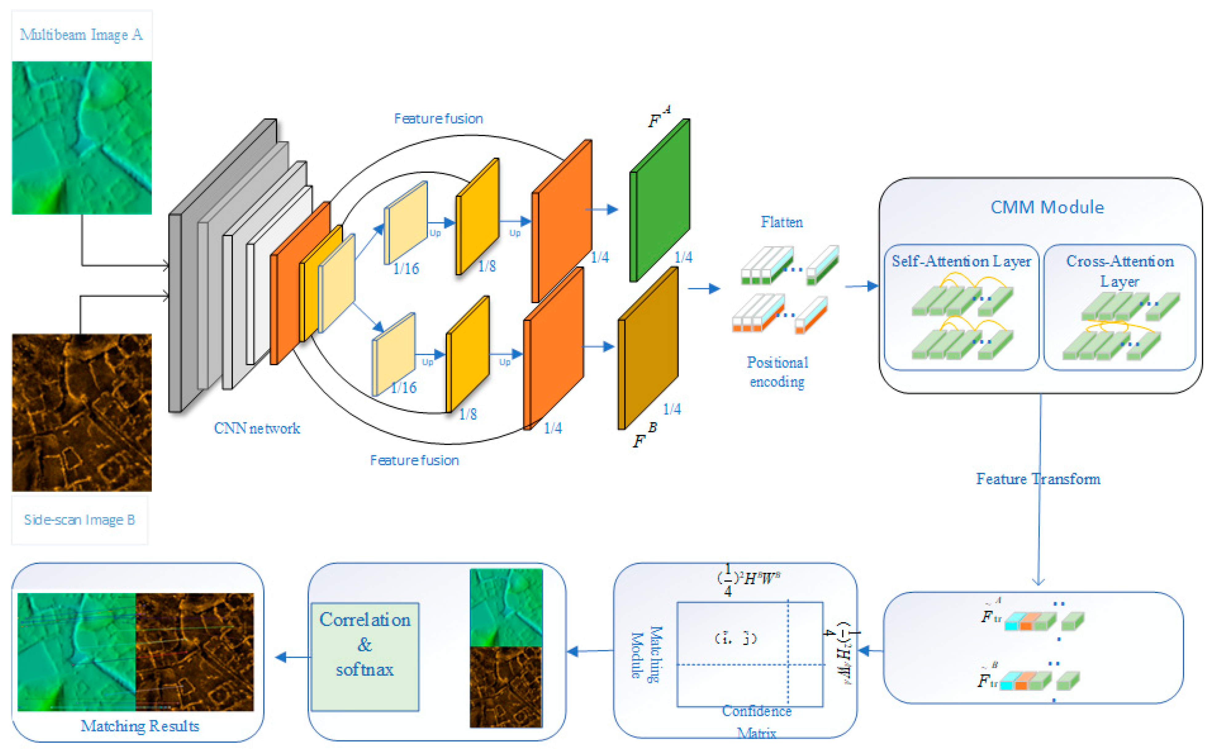
2.1. Deep Learning-Based Multi-Beam and Side-Scan Image Feature Point Matching Model

The ResNet architecture is a widely used convolutional neural network model in deep learning, known for its efficiency in feature extraction. The key feature of ResNet is the use of residual connections, which allows gradients to flow more efficiently through the network, enabling the training of deeper networks. The deep learning-based multi-beam and side-scan image feature matching network proposed in this paper is structured as shown in Figure 1. The main components include a multi-modal feature matching network based on residual networks and a feature extraction module based on attention mechanisms. The input consists of acoustic images from multi-beam and side-scan sonars.

In general, the feature matching model’s processing involves three main stages. In the first stage, the multi-beam and side-scan images are input into a feature matching network based on a residual network to extract image features of different dimensions corresponding to each. These features are then enhanced in importance through a self-attention mechanism. Following this, feature fusion is applied to integrate deeper features into shallower ones, resulting in feature maps for both multi-beam $F^A$ and side-scan images $F^B$. The second stage uses a cross-attention mechanism to combine the features of the multi-beam image with those of the side-scan image, enhancing the correlation between feature points. The third stage calculates the similarity matrix of these feature points using matrix multiplication, normalizes the similarity values via the softmax function, and finally, calculates the cosine similarity of the feature point pairs based on the normalized similarity matrix. The RANSAC algorithm is applied for evaluation to achieve feature matching and generate a matching result image. The flowchart of the specific algorithm is shown in Figure 1.

This study adopted a unified convolutional neural network architecture to train features from multi-beam and side-scan images separately. The network consists of multiple convolutional modules, an upsampling module, and a final fusion convolutional module, extracting and processing spatial features of the images layer by layer. Specifically, the feature extraction convolutional modules consist of three convolutional layers, each with 64, 128, and 256 filters, respectively, and a filter size of 3 × 3. Each convolutional layer is followed by a BatchNorm2d layer and a ReLU activation function. Then, a max-pooling layer with a stride of 2 was introduced for downsampling the feature map to reduce spatial dimensions. The upsampling module uses linear interpolation to enlarge the feature map’s resolution by adjusting the spatial scale. Finally, the fusion convolutional module integrated features from different levels using a convolutional layer with 512 filters and a filter size of 3 × 3, achieving feature fusion and refined expression.

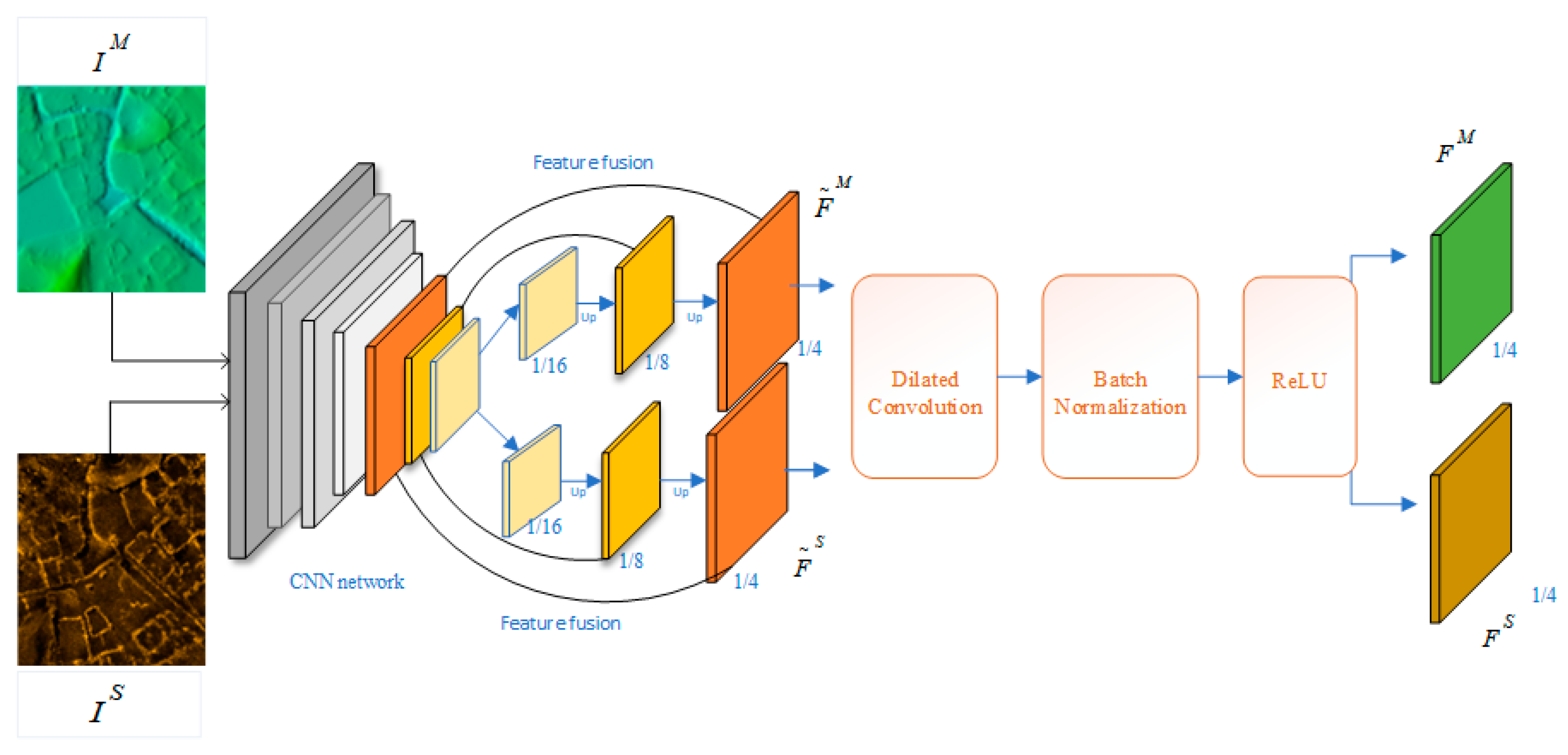
2.1.1. Feature Extraction

Due to significant differences in imaging mechanisms, bands, and time phases, multi-beam and side-scan images exhibit substantial disparities in their radiometric and geometric features. These differences make traditional matching operators based on gradients, intensities, and statistical information often ineffective in producing stable results [28,29,30]. This study selected ResNet-50 as the backbone of the feature extraction part of the model, and used the first seven convolutional layers of ResNet-50 to extract shared features for subsequent feature enhancement and matching [31]. ResNet-50 is a deep convolutional neural network that improves training stability and feature representation through residual connections. Its shallow convolutional layers, with smaller receptive fields, are effective in extracting low-level features, such as edges and corners from images, thereby achieving higher localization accuracy. As the network deepens, the model progressively captures more abstract global features, making it more robust to interference from heterogeneous images [32]. This setup retains both low-level and mid-level features (such as edges, textures, and shapes) while enhancing adaptability to different image sources, leading to more stable and accurate matching results. The structure of the feature extraction module in this paper is shown in Figure 2.

The specific process is as follows: First, the multi-beam image $I_M$ and the side-scan image $I_S$ to be matched were input into the convolutional neural network. The shared feature extraction was performed through the encoder part of the CNN. The images passed through the 5th, 6th, and 7th layers of the ResNet-50 network to generate multi-beam shared feature maps ${\stackrel{\sim }{F}}_M$ and side-scan shared feature maps ${\stackrel{\sim }{F}}_S$ at levels 1/4, 1/8, and 1/16 of the original image size. Then, independent feature extraction modules were used to extract modality-specific features from the shared features. Dilated convolutions were employed to expand the receptive field of the convolution kernels to capture more contextual information, further enhancing the feature representations extracted from the shared feature maps. Next, a self-attention module was used to enhance each feature map, generating feature representations that include context. Each layer of the shared feature map underwent convolution, followed by upsampling to fuse deeper features into the shallow features. Then, batch normalization (BatchNorm) was applied to the extracted features, and the ReLU activation function was used to enhance the model’s nonlinear expressive power. Finally, the fused 1/4-level multi-beam feature map $F_M$ and side-scan feature map $F_S$ were output for subsequent processing.

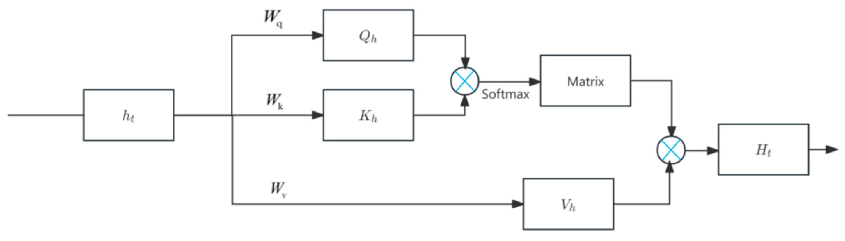
2.1.2. Attention Mechanism

This paper selects a combination of self-attention and cross-attention mechanisms. By integrating these two attention mechanisms, the model can achieve more precise keypoint selection and mutual mapping during the feature matching process [33]. The self-attention mechanism emphasizes features, such as edges or textures, in multi-beam and side-scan images to improve feature selectivity. It creates long-range dependencies between global and local image features, thereby reducing noise interference during matching. The cross-attention mechanism helps the model ignore modality differences and directly align structurally related features to recognize complementary features between multi-beam and side-scan images, allowing the model to perform more robust cross-modal matching.

Self-Attention Mechanism

Self-Attention, also known as internal attention, allows each element in an input sequence to be compared with other elements in the sequence, thereby capturing the dependencies between elements. This mechanism can dynamically capture the relationships between each position (or pixel) and other positions in the input feature map. By calculating the similarity between the representation of each position and the representations of other positions, corresponding attention weights are generated. This enables the model to focus on important information that is relevant to the current pixel [27]. Figure 3 below is a detailed flowchart, where $h_t$ represents the input vector representing the feature maps $F_M$ and $F_S$, obtained from the multi-beam and side-scan images after linear. $H_t$ is the output vector $Q_h$, $K_h$, and $V_h$ are the query vector, key vector, and value vector, respectively; $W_q$, $W_k$, and $W_v$ denote the weight matrices corresponding to the query, key, and value vectors.

The detailed process is as follows: first, the features of the input image were transformed into query ($Q$), key ($K$), and value ($V$) feature maps through three convolution operations. In this context, $Q$ represents the local feature information of a specific pixel in the multi-beam and side-scan feature maps, such as depth, intensity, or gradient. $K$ refers to the reference feature vectors (i.e., descriptors) of all pixels in the input images, providing global feature distribution information to assist $Q$ in identifying regions with high correlation. $V$ represents the feature information extracted from the relevant pixels through the attention mechanism, which is used to weight and update the input features, enhancing their representation. The specific formulas are as follows, where $W_Q$, $W_K$, and $W_V$ represent the trainable weight matrices. The relevance among each element $Wv$ in the input sequence is then measured by calculating the dot product between $Q$ and $K$, where $Q$ and $K$ represent the query and key vectors, respectively.

$$Q=X{W}_Q,K=X{W}_K,V=X{W}_V$$

(1)

Next, the similarity between each query and all keys was computed, and attention weights were generated based on these similarities. Then, batch matrix multiplication was used to calculate the dot product matrix between each $Q$ and all $K$s. The softmax function was applied to normalize the result into a probability distribution, yielding the attention weights. Finally, the attention weights were applied to $V$, and the new feature representation was obtained through weighted summation. A residual connection was used to add this output to the original input feature map, forming the final output. The formula for self-attention is as follows:

$$attention(Q,K,V)=soft\max ({\displaystyle \frac{Q{K}^T}{\sqrt{d_k}}})V$$

(2)

In the formula, $Q{K}^T$ represents the dot product between $Q$ and $K$, which computes the similarity score between each element and all other elements. The scaling factor $\sqrt{d_k}$ is used to prevent the dot product value from becoming too large, which could lead to vanishing or exploding gradients. Here, $d_k$ is the dimension of the key, and the scaling factor helps maintain the stability of the gradients during training.

Cross-Attention Mechanism

The Cross-Attention mechanism is a widely used tool in multi-modal learning, where its core idea is to guide the attention distribution of one modality’s features based on the features of another modality, thereby achieving more precise feature alignment and extraction during the information fusion process. In this study, the $Q$, $K$, and $V$ for cross-attention come from two inputs: multi-beam images and side-scan images. The multi-beam image features were projected into $Q$ through convolution, while the side-scan image features were projected into $K$ and $V$. The attention scores were obtained by calculating the similarity between $Q$ and $K$, and these scores were then used to perform a weighted sum of the values to generate the final output feature representation. The structure is shown in Figure 4.

The operations of the cross-attention mechanism and self-attention mechanism are similar, with the main difference being in the image features they process and the way information interacts. The formula for cross-attention is shown in the following figure:

$$attention(Q,K,V)=soft\max ({\displaystyle \frac{Q{K}^T}{\sqrt{d_k}}})V$$

(3)

In the formula, $Q{K}^T$ represents the dot product between $Q$ and $K$, which computes the similarity score between each element and all other elements. The scaling factor $\sqrt{d_k}$ is used to prevent the dot product value from becoming too large, which could lead to vanishing or exploding gradients. Here, $d_k$ is the dimension of the key, and the scaling factor helps maintain the stability of the gradients during training.

2.2. Loss Function

Due to the differences in feature descriptions of heterogeneous images, it is difficult to directly use a single loss function for unified measurement. In this paper, the loss function was mainly measured by calculating the symmetric epipolar distance of the fundamental matrix. This measurement reflects the distance between two matching points relative to the epipolar line, indicating the geometric consistency of the matching point pairs [34]. Specifically, for each batch of feature points, the RANSAC algorithm was used to estimate the fundamental matrix and find the inliers that satisfy the geometric relationship. In this paper, an inlier is defined as a point pair ($p_1$, $p_2$) whose symmetric epipolar distance d($p_1$, $p_2$) is less than a predefined threshold, as illustrated in Figure 5.

$$\mathrm{inliters}=\left.\left|\left\{(p_1,p_2)\right.\right.\right|\left.d(p_1,p_2)<threshold\right\}$$

(4)

Here, $p_1$ and $p_2$ represent the feature points of the multi-beam and side-scan images, respectively. The fundamental matrix $F$ describes the geometric relationship between the two perspectives of the multi-beam and side-scan images. It is used to represent the symmetric epipolar distance of the epipolar lines mapped to the side-scan image after applying the fundamental matrix. The overall expression for the symmetric epipolar distance is as follows. Let $F{p}_1$ represent the symmetric epipolar line distance of $p_1$ after being mapped to the epipolar line in the side-scan image via the fundamental matrix $F$. Similarly, let $F^T{p}_2$ represent the symmetric epipolar line distance of $p_2$ after being mapped to the epipolar line in the side-scan image via $F$. The overall expression for the symmetric epipolar line distance is as follows:

$$\mathrm{d}(p_1,p_2)={\displaystyle \frac{{(p_2.(F{p}_1))}^2}{\left|\right|F{p}_1|{|}^2}}+{\displaystyle \frac{{(p_1.(F^T{p}_2))}^2}{\left|\right|F^T{p}_2|{|}^2}}$$

(5)

This distance measures the “closeness” of two matching points on their corresponding epipolar lines in the other image. The smaller the symmetric epipolar distance, the higher the geometric consistency between the two points. Therefore, as a loss metric, it can effectively evaluate the geometric validity of matching points, i.e., determining whether they satisfy the symmetric geometric constraint. For each batch, the geometric consistency loss is computed by accumulating the distances and then averaging them to ensure that the loss is comparable across batches. The average loss formula is as follows.

$$L{\mathrm{oss}}_{avg}={\displaystyle \frac{1}{N}}{\displaystyle \sum _{i=1}^{N}d(p_{1,i},p_{2,i})}$$

(6)

Finally, an L2 regularization term is added to the final loss function. In neural networks, L2 regularization (weight decay) imposes a constraint on the size of the parameters, thus suppressing overfitting tendencies and improving generalization ability. $\theta$ represents the i-th parameter of the model, and ${‖\theta ‖}^2$ is the square of the L2 norm of parameter ${\theta }_{\mathrm{i}}$.

$$L{\mathrm{oss}}_{reg}=\lambda {{\displaystyle \sum _{\mathrm{i}=1}^{\mathrm{n}}‖{\theta }_{\mathrm{i}}‖}}^2$$

(7)

The loss function based on combination coefficients used in this paper can balance both intensity and structural changes in the images. The smaller the function value, the higher the similarity between the two images. The final expression of the loss can be written as follows:

$$L\mathrm{oss}=L{\mathrm{oss}}_{avg}+Los{s}_{reg}$$

(8)

2.3. Evaluation Metrics

To achieve a quantitative analysis of the performance of the matching algorithm, this paper adopted several key evaluation metrics: Match Success Rate (MSR), Correct Matching Points (CMP), matching time, and Root Mean Square Error (RMSE) of image feature points to assess the structural similarity between images [35].

First, the formula for calculating the Match Success Rate is as follows:

$$MSR=C/T$$

(9)

Here, C represents the number of correctly matched point pairs, and T represents the total number of matched points. The Match Success Rate reflects the correspondence between the keypoint locations when matching the target image and the reference image. The higher the success rate, the greater the precision in coordinate location matching. Root Mean Square Error (RMSE) is an indicator that measures the difference between two sets (such as predicted values and true values, or between matching keypoints). In image processing, machine learning, and other statistical and optimization tasks [36], RMSE is commonly used to evaluate the performance of a model or the accuracy of matching. Since RMSE measures the difference in coordinates of image matching points, it can be computed by using the keypoint descriptors extracted from multi-beam and side-scan images. Its formula is as follows:

$$RMSE={\displaystyle \frac{1}{n}}\sqrt{{\displaystyle \sum _{i=1}^n({(x_{mbes}-x_{sss})}^2+{(y_{mbes}-y_{sss})}^2)}}$$

(10)

Here, $x_{mbes}$ and $y_{mbes}$ represent the coordinates of keypoints in the multi-beam image, while $x_{sss}$ and $y_{sss}$ represent the corresponding keypoint coordinates in the side-scan image. By comparing the RMSE values, the accuracy of the matching can be determined. A smaller RMSE value indicates a smaller geometric error of the matching points, and thus, better matching performance.

3. Experimental Area and Data

3.1. Experimental Area

The experimental area of this study is located in the Shicheng area of Qiandao Lake, which is known for its unique topography due to the underwater ancient city ruins. The underwater terrain is quite complex, containing structures, such as ancient city walls, streets, and building remnants. The water depth ranges from 30 to 40 m, providing a diverse substrate environment for the experiment. The unique topographical features of the Shicheng area are suitable for verifying the registration effects of multi-beam and side-scan sonar data [37]. In the experimental design, the survey lines cover different types of terrain within the ruins to ensure data diversity, thereby thoroughly evaluating the applicability and robustness of the registration methods used.

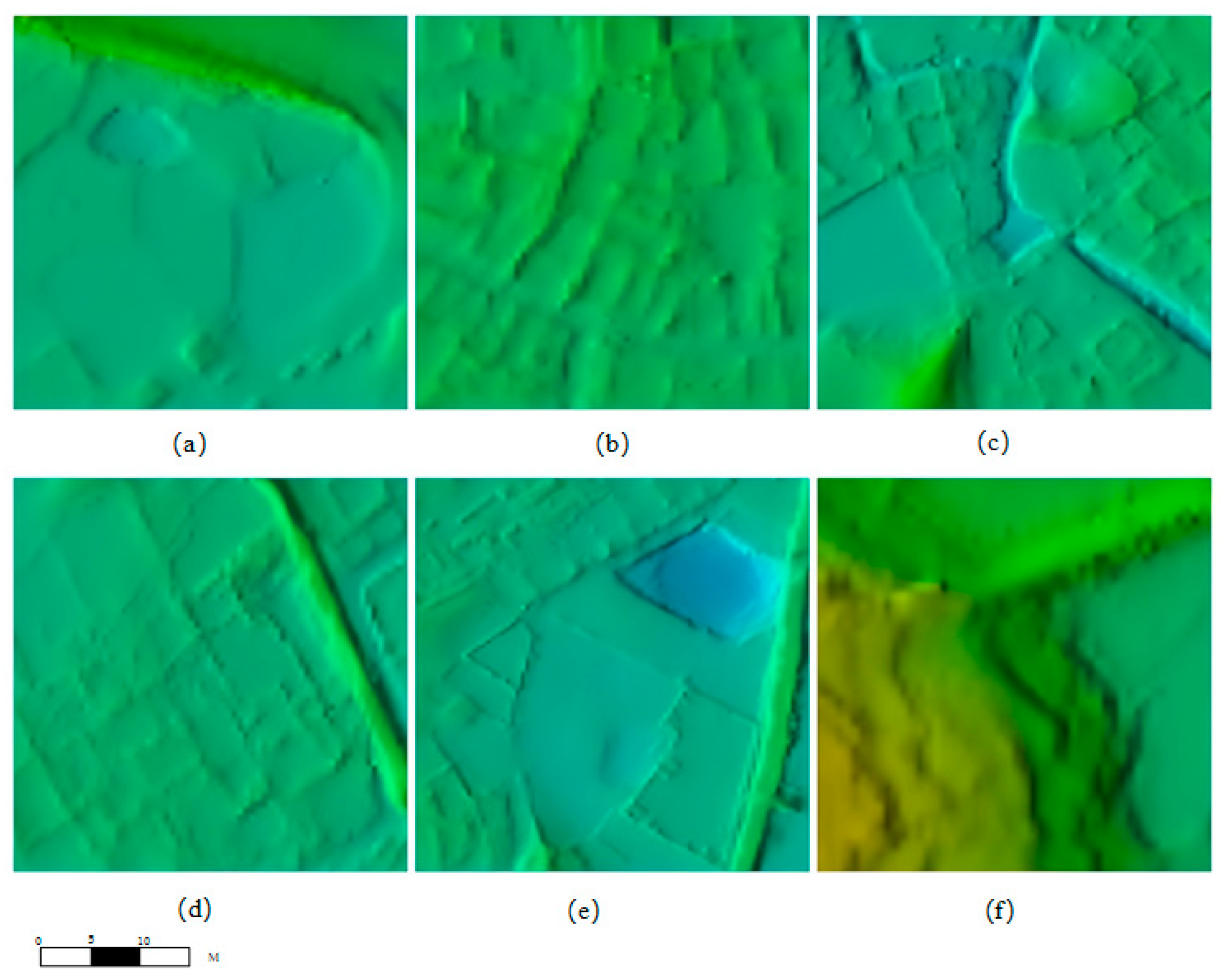
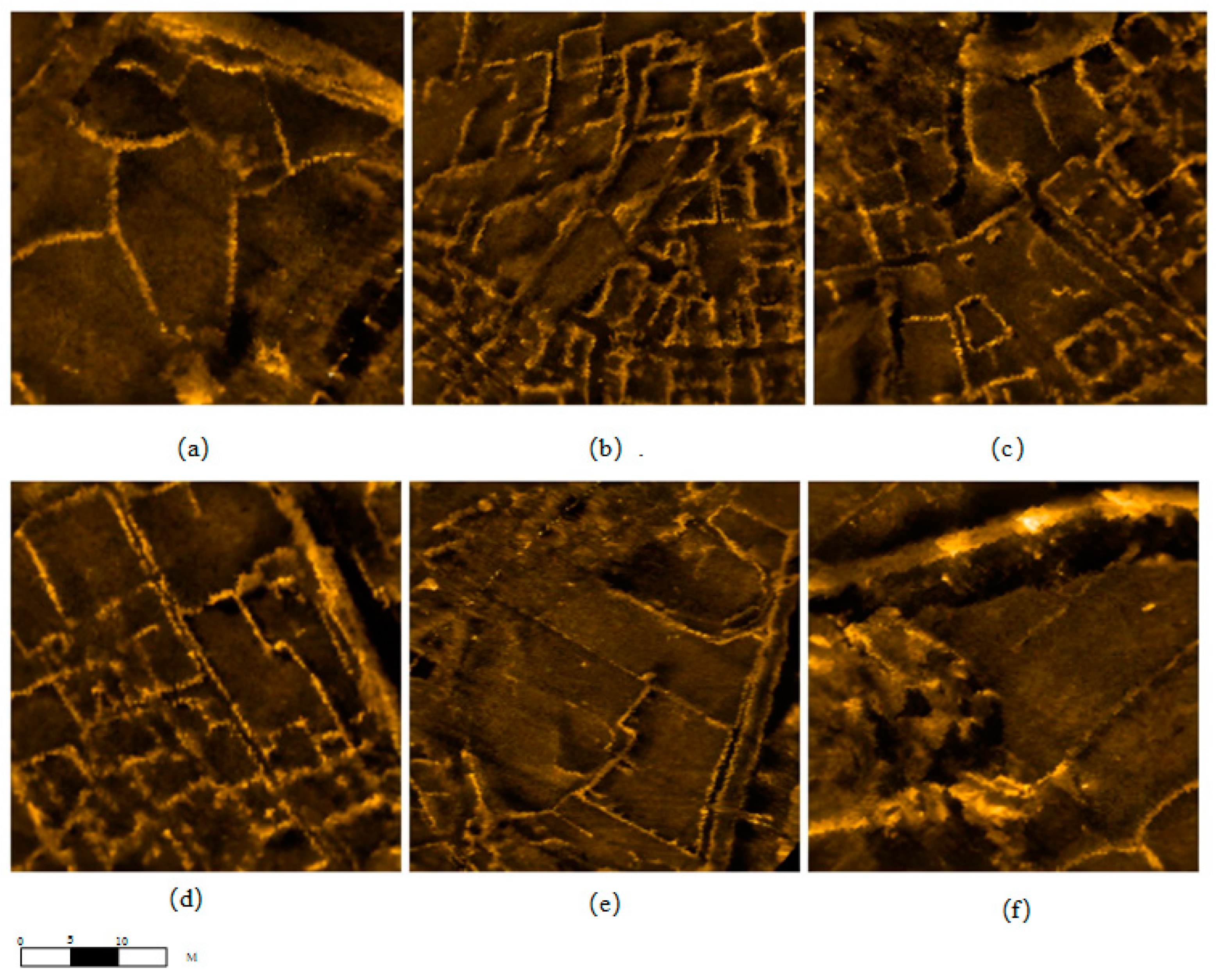
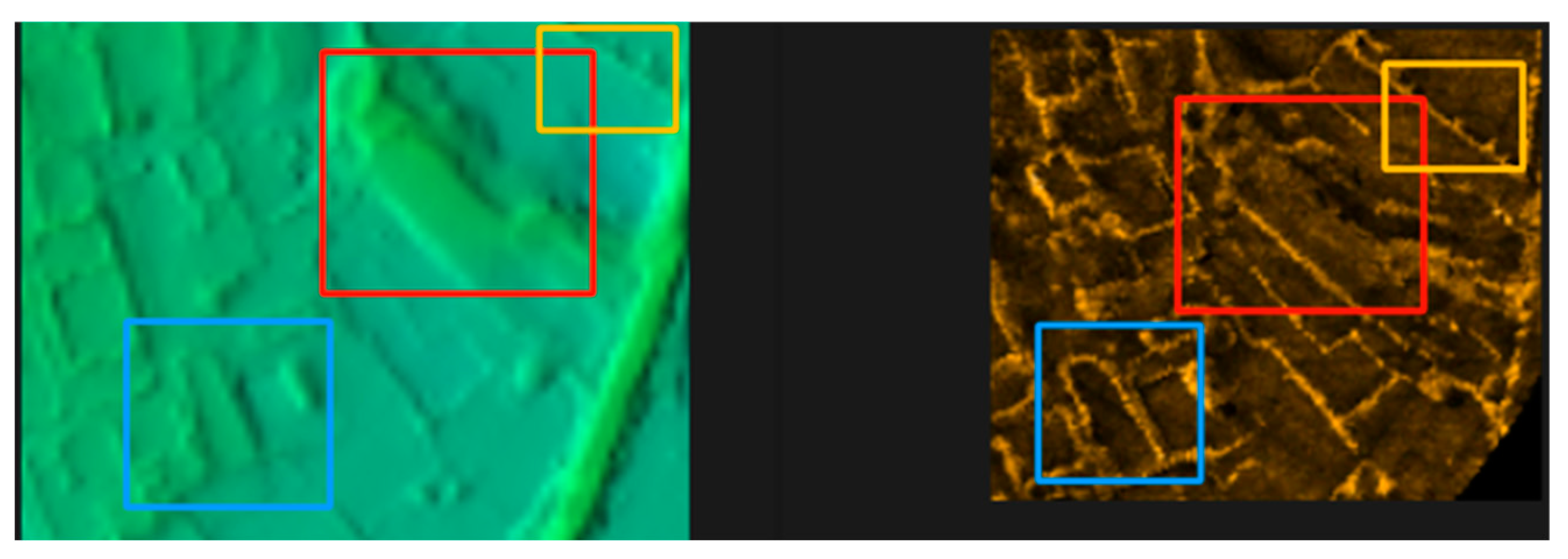
3.2. Experimental Data

The data for this study were sourced from an archaeological survey conducted in the Qiandao Lake area, collected in October 2023. The data include side-scan sonar data obtained by the HaiZhuoTongChuang 3060 side-scan system (HaiZhuoTongChuang, Guangzhou, China) and multi-beam data collected by the R2Sonic 2024 (R2Sonic, Houston, TX, USA) and Reson 7125 (Reson, Slangerup, Denmark) shallow-water multi-beam systems. The multi-beam system is fixed onboard the vessel, and through navigation positioning, data import, processing, filtering, and mapping, a point cloud map of the multi-beam data is generated. In contrast, the side-scan sonar system is installed using a towed configuration, providing a wider scanning range. During data processing, the side-scan sonar data undergo decoding, bottom tracking, distortion correction, attitude correction, and georeferencing interpolation to produce side-scan images that accurately reflect the seabed conditions. To reduce the impact of the complex underwater environment on image feature recognition, the experimental area is divided into several smaller regions, and feature matching is performed within these regions. This division helps to minimize the interference from factors, such as lighting variations, noise, and seabed terrain differences, thereby improving the matching accuracy. The processed multi-beam and side-scan image samples of smaller regions are shown in Figure 6 and Figure 7.

From Figure 6a,d and Figure 7a,d, it can be observed that due to the significant differences in the imaging methods of multi-beam and side-scan images, the pixel gradient changes are not obvious, especially in multi-beam images where the edges are relatively blurry. The feature differences between the two are substantial, making effective matching challenging. From Figure 6b and Figure 7b, it is evident that the distortion in the lower part of the images is significant, and the resolution of the multi-beam images is relatively low, accompanied by a large amount of noise, further affecting the matching results. Figure 6c and Figure 7c show iconic structures, but due to missing data in the side-scan images during stitching caused by factors, such as water disturbance, there is a noticeable gap compared to the multi-beam images, increasing the difficulty of matching. Furthermore, in Figure 6e and Figure 7e, the structure of the lake is clearly visible in the multi-beam images, while the side-scan images lack certain data. If feature matching can accurately correspond, it will help further analyze the geomorphological features of the study area. Finally, in Figure 6f and Figure 7f, there is a noticeable difference in brightness, and the matching of the mountain and wall areas also faces challenges due to difficulty in aligning feature points, making conventional feature matching methods unable to yield effective results.

3.3. Dataset Construction

The difficulty and cost of obtaining underwater observation data are significantly higher compared to other data acquisition methods. Furthermore, acquiring the true attributes of the observed objects is even more costly. Therefore, the issue of insufficient data in underwater sonar image research cannot be ignored and is expected to persist. In addition, these two types of data have significant differences due to their imaging principles. This difference in imaging methods leads to significant variations in how the same seafloor area is represented in both images. Moreover, due to the different perspectives, multi-beam images are typically obtained from a vertical view of the seafloor, while side-scan sonar images are captured from a lower lateral angle. This perspective difference also results in variations in the shape and position of the same objects in the two images. Furthermore, their resolutions differ, and common sonar image issues, such as noise, shadow effects, and other distortions, manifest differently in these two imaging systems, further complicating the image registration process. In Figure 8, the blue, red, and yellow boxes clearly show the different transformation relationships. When the detected feature points only have a single transformation, the error is small. However, when multiple transformations exist in one area, using a single transformation formula may cause the program to fail. Therefore, to ensure the model can accurately learn the feature point matching process, the training set data must be processed to ensure they maintain a consistent transformation relationship as much as possible.

In response to the current lack of corresponding multi-beam echosounder and side-scan sonar image datasets, this study has established a dataset containing images from both multi-beam and side-scan sonars. This dataset not only meets the sample quantity requirements for training but also includes sonar images captured from various imaging angles, which helps improve the generalization ability of the network model. Due to differences in the image acquisition methods and variations in the image coverage, we have filtered the images to ensure they are mostly from the same region. Moreover, because side-scan sonar images are heavily influenced by water flow and ship motion, some images suffer from deformation and misalignment, which further affects the imaging quality after geographic mosaicking. Therefore, these poor-quality images have been excluded, as shown in Figure 9.

In addition, since the network model requires the multi-beam and side-scan images to come from the same region and remain as consistent as possible, preliminary image registration of the acquired multi-beam and side-scan images is necessary. Specifically, through multiple rounds of manual point selection, we roughly determine the correspondence between the multi-beam and side-scan images and then calculate the perspective transformation matrix for both images at this stage. Subsequently, based on the obtained perspective transformation matrix, matrix transformations are applied to the side-scan images using the multi-beam images as the reference. This process completes the alignment and segmentation of the images. Regions of interest (ROI) are then selected and cropped, resulting in nearly one-to-one corresponding slices of multi-beam and side-scan images. To enhance the model’s practicality, we also performed rotation and brightness adjustments on some of the multi-beam and side-scan images to simulate changes from different perspectives. Figure 10 displays parts of the processed dataset.

4. Results and Analysis

4.1. Experimental Setup

The experiment was conducted on a deep learning platform based on PyTorch, with hardware configuration, including an NVIDIA 4060 GPU, Intel i9-12900H processor, and 16 GB of memory. The software environment was based on the vs. Code development platform. The CUDA version was 11.6, and Python version was 3.9.12. To align the custom dataset with the open-source dataset, all input images were resized to 428 × 428 pixels. The learning rate was set to 0.005, and the Adam optimizer was used for model optimization. Additionally, to prevent overfitting, the dropout value was set to 0.6.

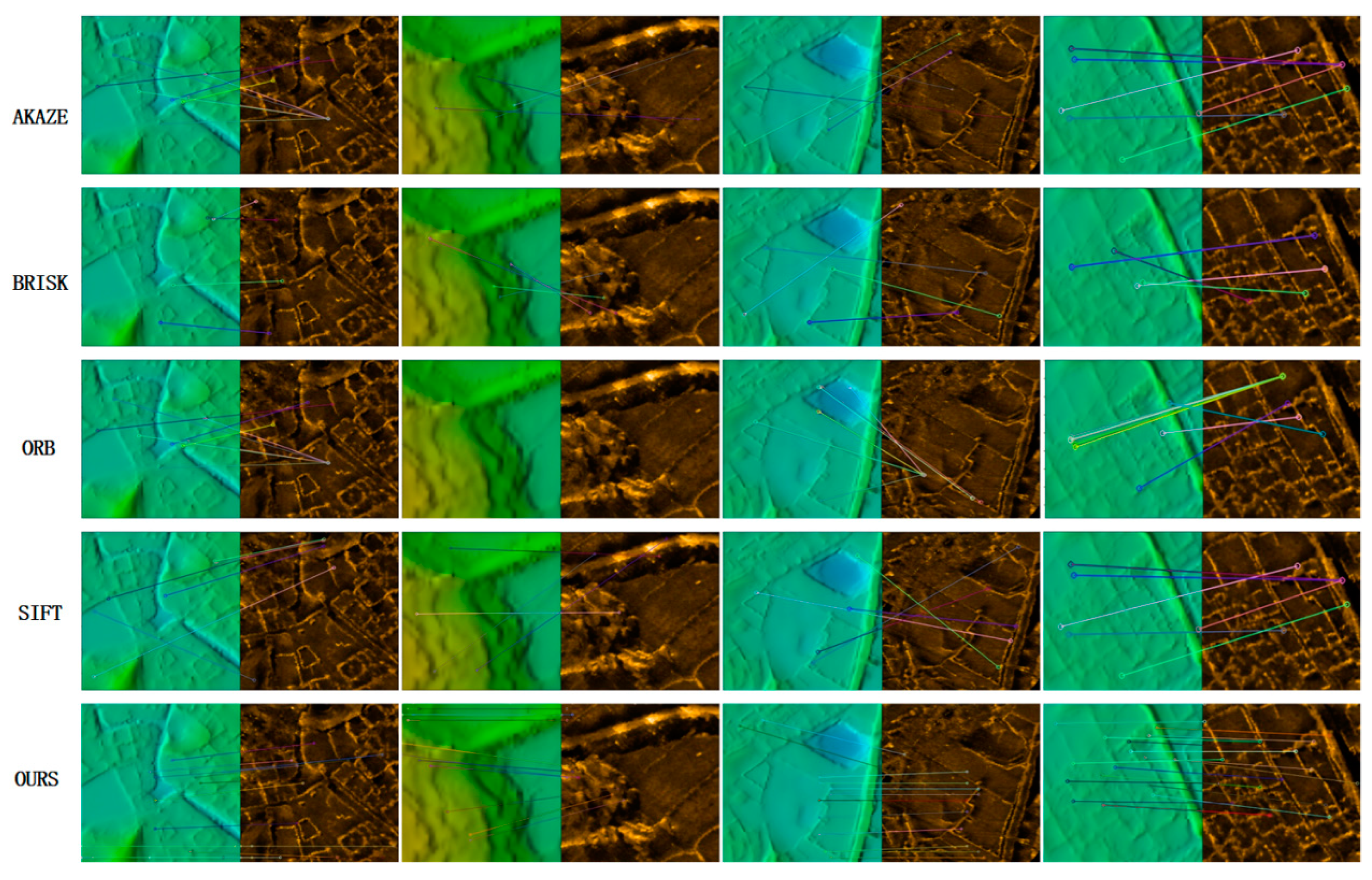
4.2. Image Matching Experiment

To validate the effectiveness of the proposed model, 1000 pairs of side-scan sonar and multi-beam bathymetric sonar images from the custom dataset were used as the training set. The model trained on this dataset was validated on a separate dataset on a separate test set. Traditional feature matching algorithms, such as SIFT, ORB, AKAZE, and BRISK, were selected as baseline comparison methods. Traditional feature matching algorithms, including SIFT, ORB, AKAZE, and BRISK, were selected as benchmark comparisons. Among them, SIFT (Scale-Invariant Feature Transform) is widely used in image matching, with invariance to translation, rotation, and scaling [38]; ORB (Oriented FAST and Rotated BRIEF) is an efficient feature extraction algorithm that combines FAST feature detection and the BRIEF descriptor, making it suitable for image matching [39]; AKAZE (Accelerated KAZE) improves scale invariance using nonlinear scale spaces and acceleration techniques, making it suitable for image matching [40]; BRISK (Binary Robust Invariant Scalable Keypoints) is based on binary descriptors, offering both scale and rotation invariance, which is ideal for efficient image matching tasks [41].

Several image groups with different feature variations were selected from the dataset for testing, including scenes, such as underwater lakes, buildings, ruins, and complex terrains. These image pairs contain significant noise interference and have complex measurement backgrounds, representing various typical underwater environments. The aim was to evaluate the performance of different algorithm models under complex conditions. As shown in Figure 11.

As shown in Figure 11, the matching results of different algorithms on the four pairs of test images vary significantly. Specifically, the AKAZE method identifies a small number of correct matching point pairs, and these matching points are not evenly distributed. BRISK, despite its scale and rotation invariance, can only detect a few correct matches due to the significant heterogeneity between multi-beam and side-scan images. The ORB algorithm performs poorly in the tests, even resulting in incorrect matches. The SIFT algorithm is highly dependent on local extrema points, with its descriptors often concentrated at corner points, leading to incorrect matches in certain cases. These results indicate that traditional feature matching algorithms often lack sufficient robustness when handling images with significant nonlinear differences and are ineffective at matching multi-beam and side-scan images. In

Table 1. Matching experiment data between different algorithms.

Groupings	CMP/Points	MSR/%	RMSE	Image Size	Time/s
AKAZE	11	36%	162.72	448 × 448	0.0589
BRISK	7	21.82%	149.04	448 × 448	0.0208
ORB	33	24%	118.31	448 × 448	0.0230
SIFT	14	43%	133.40	448 × 448	0.0437
Ours	29	93.12%	1.97	448 × 448	0.0100

, the Root Mean Square Error (RMSE) values of these algorithms all exceed 100, indicating poor image matching performance. This reflects significant differences between the two images in terms of content, color, and lighting. In contrast, the algorithm proposed in this study achieves an RMSE of only 1.97, demonstrating a much better matching performance between multi-beam and side-scan images.

Based on the experimental results shown in Figure 11 and Table 1, it can be observed that the algorithm proposed in this paper significantly outperforms traditional algorithms in terms of the number of matched feature points, matching success rate, and the uniformity of feature points. This is because traditional feature matching algorithms struggle to adapt to large geometric transformations, leading to unstable matching results. Furthermore, factors, such as the complex underwater environment and high levels of clutter interference, result in low image quality and contrast, making it difficult for traditional feature extraction methods to capture enough feature points, which leads to a large number of mismatches. Therefore, traditional methods are not suitable for matching multi-beam and side-scan sonar images. In contrast, the proposed algorithm leverages Transformer-based self-attention and cross-attention mechanisms to enhance the discriminative power of feature map descriptors. This allows the model to find a sufficient number of consistent feature points with matching identities, even in situations where feature points are sparse, achieving stable matching results.

4.3. Ablation Experiment Results

To evaluate the effectiveness of the attention mechanism in the feature extraction module, the following ablation experiments were set up. Under the same network architecture, the self-attention mechanism, cross-attention mechanism, and overall attention mechanism modules were removed one by one, and each network was trained using the same training data. To comprehensively demonstrate the matching performance of the model on different datasets, three types of images were selected as test data. The visualization of the registration results is shown in Figure 12.

As shown in Figure 12, the network in group C, lacking attention mechanisms, performs the worst in matching, especially in low-texture areas, where it is difficult to find corresponding feature points between the two images. In contrast, networks containing only the self-attention mechanism module (group A) and the cross-attention mechanism module (group B) perform better than group C in terms of the number of matched feature points, but they can only extract a small number of feature points in regions with more noticeable texture. The matching performance is significantly inferior to that of the mixed attention module used in our method. These results indicate that in multi-beam and side-scan image matching tasks, which involve significant nonlinear differences and geometric distortions, the attention module plays a crucial role in enhancing the network’s feature extraction capability. The experimental results demonstrate that the proposed mixed module of self-attention and cross-attention mechanisms achieves the best matching performance.

4.4. Analysis of Experimental Results

The stability of the feature matching results was verified using several randomly selected images containing various underwater targets. As shown in Figure 13, although the image quality and spatial resolution of multi-beam images are significantly lower than those of side-scan sonar images, the matched images still retain a large number of evenly distributed feature points. Specifically, for the image matching of urban areas shown in groups (a) and (d) of Figure 13, due to the rich texture in urban areas, there are more feature points, allowing for the matching of more points. According to the evaluation metrics in

Table 2. Matching experimental data in different regions.

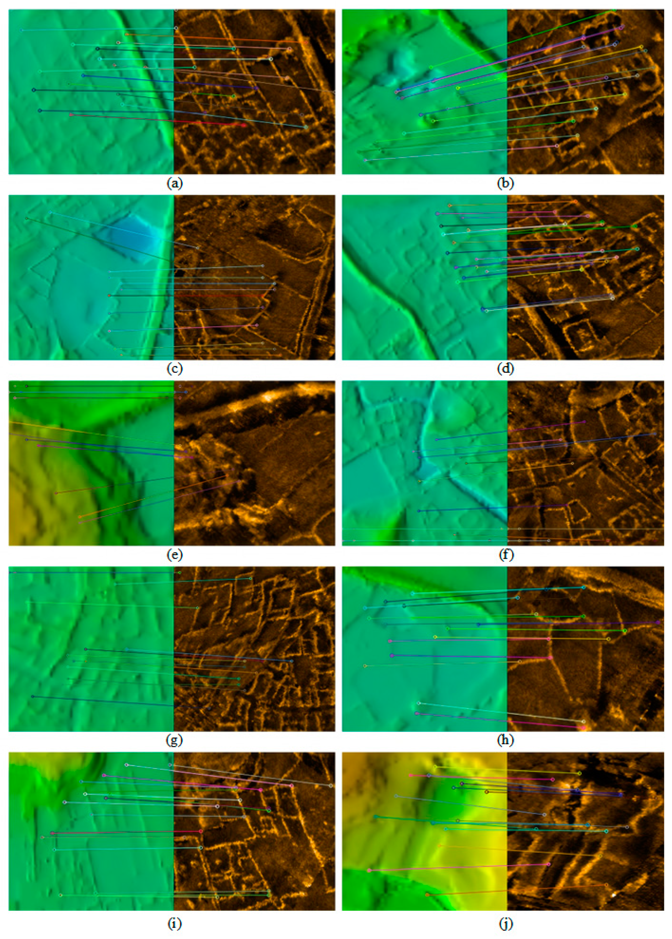
Groupings	CMP/Points	MSR/%	RMSE	Image Size	Time/s
Group a	16	93.75%	3.05	448 × 448	0.0189
Group b	40	97.45%	1.75	448 × 448	0.0100
Group c	29	81.82%	1.67	448 × 448	0.0108
Group d	26	89.85%	3.42	448 × 448	0.0100
Group e	18	80.21%	5.13	448 × 448	0.0050
Group f	46	92.62%	1.97	448 × 448	0.0015
Group g	36	89.65%	3.22	448 × 448	0.0021
Group h	20	86.00%	2.31	448 × 448	0.0005
Group i	25	91.85%	4.32	448 × 448	0.0021
Group j	26	90.21%	2.03	448 × 448	0.0012

, the RMSE value is approximately three, and the MSR value exceeds 90%, with most matched points being correct. For the hilly area images in groups (e), (j), and (c) of Figure 13, although there are fewer feature points, the MSR value exceeds 81%, and the RMSE value meets the requirements, allowing for the accurate matching of the relationship between multi-beam and side-scan images. For the images in groups (b), (g), (i), and (f) of Figure 13, although there are significant distortions and large image differences, the model is still able to extract enough feature points after training, with the RMSE value remaining at a low level and the MSR value exceeding 91%. These results indicate that the model can effectively match feature points between multi-beam and side-scan images. For images with less prominent features, such as those in groups (e), (j), and (c) of Figure 13, some surface feature information is weakened, and there is further room for improvement in the matching effect. Compared to traditional image matching methods, the proposed multi-beam and side-scan image matching method shows more feature points, a matching accuracy exceeding 80%, and faster matching speed in an interference-free environment. Overall, the proposed algorithm outperforms traditional methods in terms of accuracy and robustness.

5. Conclusions

This paper proposes a feature matching algorithm suitable for multi-beam and side-scan sonar images, which leverages self-attention and cross-attention mechanisms to enhance feature representation, thereby improving the discriminative power of descriptor vectors. The algorithm is based on the LOFTR algorithm, incorporating a residual network structure during the encoding process to strengthen the model’s deep learning capabilities, enabling more effective feature point assignment even in regions with weak textures in the images. Using a self-built training dataset for multi-beam and side-scan images, the algorithm is trained through self-supervised learning with the support of the residual network, effectively extracting and matching feature points from the images. The matching performance of the algorithm was validated through a self-constructed test set. The experimental results show that, compared to traditional feature matching algorithms, such as SIFT, ORB, AKAZE, and BRISK, the proposed model exhibits significant improvements in terms of feature point quantity, matching success rate, and the uniformity of feature point distribution. While traditional algorithms perform well on images with rich textures and the same viewpoints, their matching performance significantly deteriorates when applied to multi-modal images captured under different viewpoints and conditions, especially in underwater environments with noise and complex backgrounds. However, the experiments also reveal some limitations of the proposed method. For certain images with shallow features or low texture, the matching performance is slightly lower than expected, and the RMSE value is relatively large. Following our analysis, we hypothesize that this issue may arise from the deep convolutional layers insufficiently preserving shallow features. Future research will focus on enhancing the feature extraction structure by incorporating additional layers in the shallow network or integrating more flexible multi-scale feature extraction modules, with the goal of further improving the model’s adaptability to complex and dynamic environments.

Due to the difficulty and high cost of acquiring underwater observation data, there are still relatively few available multi-beam and side-scan datasets that meet the required conditions. Therefore, efforts are being actively made to collect new datasets from other regions to further carry out generalization research. These new datasets will support the verification of the algorithm’s applicability under different environments and conditions and help enhance the algorithm’s robustness and accuracy in diverse underwater scenarios. Additionally, future research will focus on optimizing the feature extraction structure to further improve matching stability in low-texture images and high-noise environments, with the aim of expanding the algorithm’s application potential in broader computer vision tasks, such as multi-beam and side-scan image matching and fusion.

In conclusion, the proposed algorithm demonstrates good matching performance and time efficiency for underwater multi-modal image matching tasks and proves its superiority in accuracy and robustness. Future research will aim to optimize the feature extraction structure and further improve the matching stability in low-texture images and high-noise environments, with the aim of enhancing its applicability to a wider range of computer vision tasks, such as multi-beam and side-scan image matching and fusion; the model’s potential will be further explored and expanded.

References

- Hu, Y.; Liu, Y.; Ding, J.; Liu, B.; Chu, Z. Regional archaeological underwater survey method: Applications and implications. Archaeol. Prospect. 2022, 29, 607–622. [Google Scholar] [CrossRef]
- Reggiannini, M.; Salvetti, O. Seafloor analysis and understanding for underwater archeology. J. Cult. Herit. 2017, 24, 147–156. [Google Scholar] [CrossRef]
- Dura, E.; Zhang, Y.; Liao, X.; Dobeck, G.J.; Carin, L. Active learning for detection of mine-like objects in side-scan sonar imagery. IEEE J. Ocean. Eng. 2005, 30, 360–371. [Google Scholar] [CrossRef]
- Wu, Z.; Yang, F.; Luo, X.; Li, S. High-Resolution Submarine Topography—Theory and Technology for Surveying and Post-Processing; Science PressEditor: Beijing, China, 2017. [Google Scholar]
- Lazaridis, G.; Petrou, M. Image registration using the Walsh transform. IEEE Trans. Image Process 2006, 15, 2343–2357. [Google Scholar] [CrossRef]
- Yang, F.; Wu, Z.; Du, Z.; Jin, X. Co-registering and Fusion of Digital Information of Multi-beam Sonar and Side-scan Sonar. Geomat. Inf. Sci. Wuhan Univ. 2006, 31, 740–743. [Google Scholar]
- Riyait, V.S.; Lawlor, M.A.; Adams, A.E.; Hinton, O.R.; Sharif, B.S. A review of the ACID synthetic aperture sonar and other sidescan sonar systems. Int. Hydrogr. Rev. 1995, 72, 285–314. [Google Scholar]
- Mayer, L.; Jakobsson, M.; Allen, G.; Dorschel, B.; Falconer, R.; Ferrini, V.; Lamarche, G.; Snaith, H.; Weatherall, P. The Nippon Foundation—GEBCO seabed 2030 project: The quest to see the world’s oceans completely mapped by 2030. Geosciences 2018, 8, 63. [Google Scholar] [CrossRef]
- Blondel, P. The Handbook of Sidescan Sonar; Springer Science & Business Media: Berlin/Heidelberg, Germany, 2010. [Google Scholar]
- Cobra, D.T.; Oppenheim, A.V.; Jaffe, J.S. Geometric distortions in side-scan sonar images: A procedure for their estimation and correction. IEEE J. Ocean. Eng. 1992, 17, 252–268. [Google Scholar] [CrossRef]
- Clarke, J.E.H. Dynamic motion residuals in swath sonar data: Ironing out the creases. Int. Hydrogr. Rev. 2003, 4. [Google Scholar]
- Cervenka, P.; de Moustier, C.; Lonsdale, P.F. Geometric corrections on sidescan sonar images based on bathymetry. Application with SeaMARC II and Sea Beam data. Mar. Geophys. Res. 1995, 17, 217–219. [Google Scholar] [CrossRef]
- Cervenka, P.; de Moustier, C. Postprocessing and corrections of bathymetry derived from sidescan sonar systems: Application with SeaMARC II. IEEE J. Ocean. Eng. 1994, 19, 619–629. [Google Scholar] [CrossRef]
- Zhao, J.; Wag, J. Study on Fusion Method of the Block Image of MBS and SSS. Geomat. Inf. Sci. Wuhan Univ. 2013, 38, 287–290. [Google Scholar]
- Chen, G.; Mao, Z.; Shen, J. Advanced Object Detection in Multibeam Forward-Looking Sonar Images Using Linear Cross-Attention Techniques. In Proceedings of the 2024 IEEE International Conference on Image Processing (ICIP), Abu Dhabi, United Arab Emirates, 27–30 October 2024; IEEE: Piscataway, NJ, USA, 2024; pp. 1026–1031. [Google Scholar]
- Schimel, A.C.; Beaudoin, J.; Parnum, I.M.; Le Bas, T.; Schmidt, V.; Keith, G.; Ierodiaconou, D. Multibeam sonar backscatter data processing. Mar. Geophys. Res. 2018, 39, 121–137. [Google Scholar] [CrossRef]
- Lucieer, V.; Roche, M.; Degrendele, K.; Malik, M.; Dolan, M.; Lamarche, G. User expectations for multibeam echo sounders backscatter strength data-looking back into the future. Mar. Geophys. Res. 2018, 39, 23–40. [Google Scholar] [CrossRef]
- Le Bas, T.P.; Huvenne, V. Acquisition and processing of backscatter data for habitat mapping-comparison of multibeam and sidescan systems. Appl. Acoust. 2009, 70, 1248–1257. [Google Scholar] [CrossRef]
- Mitchell, G.A.; Orange, D.L.; Gharib, J.J.; Kennedy, P. Improved detection and mapping of deepwater hydrocarbon seeps: Optimizing multibeam echosounder seafloor backscatter acquisition and processing techniques. Mar. Geophys. Res. 2018, 39, 323–347. [Google Scholar] [CrossRef]
- Fakiris, E.; Blondel, P.; Papatheodorou, G.; Christodoulou, D.; Dimas, X.; Georgiou, N.; Kordella, S.; Dimitriadis, C.; Rzhanov, Y.; Geraga, M. Multi-frequency, multi-sonar mapping of shallow habitats—Efficacy and management implications in the national marine park of Zakynthos, Greece. Remote Sens. 2019, 11, 461. [Google Scholar] [CrossRef]
- Zhou, X.; Yu, C.; Yuan, X.; Luo, C. A Matching Algorithm for Underwater Acoustic and Optical Images Based on Image Attribute Transfer and Local Features. Sensors 2021, 21, 7043. [Google Scholar] [CrossRef]
- Aykin, M.D.; Negahdaripour, S. On feature matching and image registration for two-dimensional forward-scan sonar imaging. J. Field Robot. 2013, 30, 602–623. [Google Scholar] [CrossRef]
- ZHANG Ning, J.S.B.G. An iterative and adaptive registration method for multi-beam and side-scan sonar images. Acta Geod. Et. Cartogr. Sin. 2022, 51, 1951–1958. [Google Scholar]
- Shang, X.J.Z. Obtaining High-Resolution Seabed Topography and Surface Details by Co-Registration of Side-Scan Sonar and Multibeam Echo Sounder Images. Remote Sens. 2019, 11, 1496. [Google Scholar] [CrossRef]
- Wynn, W.; Frahm, C.; Carroll, P.; Clark, R.; Wellhoner, J.; Wynn, M. Advanced superconducting gradiometer/magnetometer arrays and a novel signal processing technique. IEEE Trans. Magn. 1975, 11, 701–707. [Google Scholar] [CrossRef]
- Revaud, J.; De Souza, C.; Humenberger, M.; Weinzaepfel, P. R2d2: Reliable and repeatable detector and descriptor. Adv. Neural Inf. Process. Syst. 2019, 32. [Google Scholar]
- Sun, J. LoFTR: Detector-Free Local Feature Matching with Transformers. In Proceedings of the IEEE/CVF Conference on Computer Vision and Pattern Recognition, Nashville, TN, USA, 20–25 June 2021. [Google Scholar] [CrossRef]
- Honghua, J. Research on UAV remote sensing image registration based on BBF optimization algorithm. Comput. Meas. Control 2023, 32, 232–237. [Google Scholar]
- Xiang, H.; Xuefei, L.; Yineng, L.I. Heterogeneous Image Matching Algorithm Based on Feature Fusion. Navig. Control 2023, 22, 106–115. [Google Scholar]
- LAN Chaozhen, L.W.Y.J. Deep learning algorithm for feature matching of cross modality remote sensing images. Acta Geod. Et. Cartogr. Sin. 2021, 50, 189–202. [Google Scholar]
- Shafiq, M.; Gu, Z. Deep residual learning for image recognition: A survey. Appl. Sci. 2022, 12, 8972. [Google Scholar] [CrossRef]
- Song, Z.L. Remote Sensing Image Registration Based on Retrofitted SURF Algorithm and Trajectories Generated From Lissajous Figures. IEEE Geosci. Remote Sens. Lett. 2010, 7, 491–495. [Google Scholar] [CrossRef]
- Yu, C.; Li, S.; Feng, W.; Zheng, T.; Liu, S. SACA-fusion: A low-light fusion architecture of infrared and visible images based on self- and cross-attention. Vis. Comput. 2024, 40, 3347–3356. [Google Scholar] [CrossRef]
- Ben-Artzi, G.; Halperin, T.; Werman, M.; Peleg, S. Epipolar geometry based on line similarity. In Proceedings of the 2016 23rd International Conference on Pattern Recognition (ICPR), Cancun, Mexico, 4–8 December 2016; IEEE: Piscataway, NJ, USA, 2016; pp. 1864–1869. [Google Scholar]
- Carion, N.; Massa, F.; Synnaeve, G.; Usunier, N.; Kirillov, A.; Zagoruyko, S. End-to-end object detection with transformers. In European Conference on Computer Vision; Springer: Berlin/Heidelberg, Germany, 2020; pp. 213–229. [Google Scholar]
- Deshmukh, M.; Bhosle, U. A survey of image registration. Int. J. Image Process. 2011, 5, 245. [Google Scholar]
- Yang, F.; Xu, F.; Zhang, K.; Bu, X.; Hu, H.; Anokye, M. Characterisation of terrain variations of an underwater ancient town in Qiandao Lake. Remote Sens. 2020, 12, 268. [Google Scholar] [CrossRef]
- Wei, M.; Xiwei, P. WLIB-SIFT: A Distinctive Local Image Feature Descriptor. In Proceedings of the 2019 IEEE 2nd International Conference on Information Communication and Signal Processing (ICICSP), Weihai, China, 28–30 September 2019; IEEE: Piscataway, NJ, USA, 2019; pp. 379–383. [Google Scholar]
- Justinn Barr, R.G.L.W. The Drosophila CPEB Protein Orb Specifies Oocyte Fate by a 39UTR-Dependent Autoregulatory Loop. Genetics 2019, 213, 1431–1446. [Google Scholar] [CrossRef] [PubMed]
- Yabuta, S.Y.Y. Solution for Corresponding Problem of Stereovision By Using AKAZE features. In Proceedings of the 2020 21st International Conference on Research and Education in Mechatronics (REM), Cracow, Poland, 9–11 December 2020. [Google Scholar]
- Liu, Y.; Zhang, H.; Guo, H.; Xiong, N.N. A FAST-BRISK Feature Detector with Depth Information. Sensors 2018, 18, 3908. [Google Scholar] [CrossRef]