High-Resolution Reconstruction of Total Organic Carbon Content in Lake Sediments Using Hyperspectral Imaging

Abstract

The total organic carbon (TOC) content in lake sediments is an effective archive indicating past climate changes. However, the resolution of the TOC record has generally been limited by factors such as subsampling intervals, hampering further comprehension of past climate change. Recently, hyperspectral imaging technology has been increasingly employed to scan lake sediment cores, presenting new opportunities to reconstruct high-resolution sequences, but the reconstruction of long-term high-resolution TOC records using hyperspectral imaging and the climate implications have not been well studied. In this study, we scanned sedimentary cores from Wudalianchi Crater Lake in northeast China with a spatial resolution of 400 × 400 μm, utilizing visible and near-infrared (VNIR) hyperspectral imaging technology. Then, a partial least-squares regression (PLSR) model was constructed by comparing eight different preprocessing methods and optimally selecting the best spectral subset combined with a genetic algorithm (GA). Our analysis demonstrates that the PLSR model, constructed using 62 relevant bands selected by the Savitzky–Golay second derivative (D2) preprocessing method and GA, was the most reliable, with the validation set’s R-value reaching a high of 0.91 and RMSE as low as 1.18%. Notably, the spectral range of 656–669 nm showed a strong positive correlation with measured TOC, indicating its sensitivity for TOC estimation. Given this advantage, we reconstructed the TOC records of sediments from the Wudalianchi Crater Lake during the 38–13 ka BP period, which exhibited significant millennial-scale fluctuation events. These corresponded well with the millennial-scale events in pollen and TOC from Lake Sihailongwan, δ¹⁸O records of Greenland ice cores, and δ¹⁸O records from Asian stalagmites. Thus, the combination of hyperspectral imaging and the PLSR model is effective in reconstructing high-resolution TOC changes in lake sediments, which is essential for understanding climate change as well as carbon burial in lakes.

1. Introduction

Lake sediments have the advantage of continuity and high resolution, making them an ideal archive for studying past environmental and anthropogenic changes [1,2,3,4,5]. The total organic carbon (TOC) content is a crucial environmental and ecological indicator in lake sediments. It is related to exogenous inputs, lake productivity, and preservation conditions, which often indicate the status of lake basin vegetation and the influx of exogenous detrital material [6,7]. Meanwhile, TOC has also been employed to reconstruct historical regional temperature and precipitation variations [8,9]. Reconstructing high-resolution TOC changes from lake sediments is crucial for studying climate and environment variations, as well as the history of human activities [10,11,12]. However, traditional methods of determining TOC in lake sediments require subsampling, which is labor-intensive and time-consuming, destructive to sediment cores, and generally yields low resolution (with subsampling intervals often exceeding 0.5 cm). These limitations hinder the capture of high-resolution data on environmental changes, especially for extreme events with short timescales, which consequently restricts further studies of environmental changes.

Over the last decade, visible, near-infrared, and short-wavelength infrared (SWIR) spectroscopy have been widely used to scan lake sediments, as these methods are cost-effective and non-destructive while offering high-resolution records [13,14,15]. Spectral scanning identifies the composition of scanned substances based on the principles of absorption, scattering, and reflectance properties of material molecules. By analyzing the different spectral data of lake sediments, researchers have successfully obtained high-resolution records of grain size [16,17,18], chlorophyll [19,20], charcoal [21], and organic matter [22]. This technique was also utilized to detect tephra layers in sediment cores [23]. However, the reconstruction of long-term TOC records for lake sediments using hyperspectral scanning techniques is scarce, and there is a lack of comparative analysis with high-resolution climate records.

In this study, we analyzed continuous sediment core samples from Wudalianchi Crater Lake, northeast China, using visible and near-infrared (VNIR) hyperspectral imaging. We aimed to perform the following: (1) compare the effects of eight preprocessing methods on band selection for a partial least-squares regression (PLSR) model; (2) select the optimal spectral subset from the full range of raw spectra using the genetic algorithm (GA) and analyze the relationship between TOC and each band in the optimal spectral subset; and (3) compare the TOC reconstructed by the PLSR model with other paleoclimate records to assess its reliability and accuracy.

2. Materials and Methods

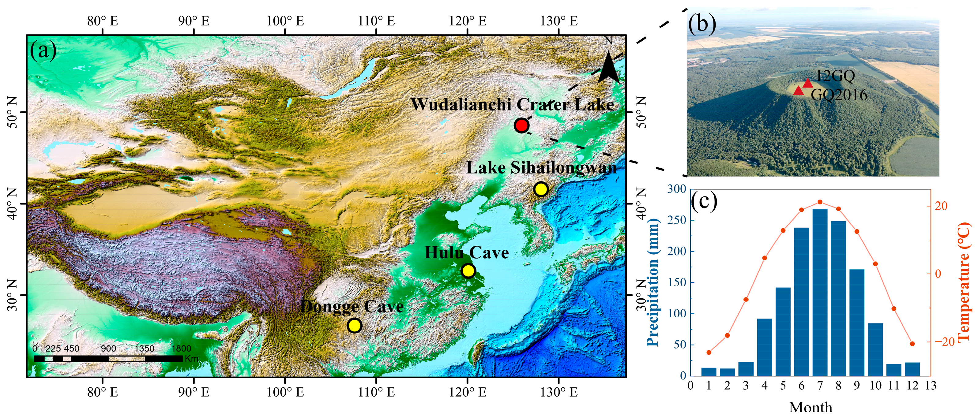
2.1. Study Area

Wudalianchi Crater Lake (48°74′N, 126°00′E) is a small and enclosed crater lake located in the Wudalianchi Global Geopark, Heilongjiang Province, in northeast China (Figure 1a,b). The lake has a surface diameter of ~400 m, a total area of 6.8 × 10⁴ m², and an elevation of 596.9 m. The lake has no obvious riverine inputs, and it is mainly replenished by surface and subsurface runoff from a catchment area of only ~0.1 km² [24]. Our study site, situated in a temperate monsoon zone, is characterized by distinct seasonal variations, with an annual average temperature of 0–0.5 °C and average precipitation of ~470 mm. The maximum temperature and precipitation occur in June, July, and August (Figure 1c). The surrounding vegetation primarily consists of mixed coniferous and broadleaf forests, dominated by birch, poplar, and larch [25].

2.2. Sample Collection

Two sediment cores, 12GQ (800 cm) and GQ2016 (2115 cm), were collected from the Wudalianchi Crater Lake in 2012 and 2016, respectively, using 5.5 cm and 9 cm diameter percussion corers. After retrieval, the cores were vertically split into two halves. One half was subsampled at 1 cm intervals, with a thickness of 1 cm, and the samples were preprocessed by air-drying, photographing, and picking out residues. The other half was stored in a refrigerated environment (~4 °C) for hyperspectral scanning [26].

2.3. Geochemical and Physical Analysis

The samples were treated with 1 mol/L of HCl to remove carbonate minerals, washed with distilled water to eliminate any remaining HCl, dried at 60 °C, and weighed. The TOC of the core 12GQ was measured using an elemental analyzer (Elementar vario MACRO cube) at the Laboratory Centre for Physical and Chemical Science, University of Science and Technology of China, with an analytical error of less than 0.1% [27].

The sediment lightness of cores 12GQ and GQ2016 was measured using a Coloreader CR-700R ultraviolet/visible spectrophotometer at the School of Earth and Space Science, University of Science and Technology of China. The results were converted to Commission Internationale De L’ Eclairage (CIE) units (L*, a*, b*), where CIE L* represents sediment lightness with a measurement error of 0.5–1% [28].

2.4. VNIR Hyperspectral Scanning

To minimize the potential effects of surface roughness on the spatial resolution, we flattened the surface of core GQ2016 before scanning it with a SPECIM FX10 hyperspectral detector (Beijing Yudecheng Technology Co., Ltd., Beijing, China). The detector employs a line-array push-scan imaging method with a VNIR spectral range of 400–1000 nm, encompassing 224 bands, and a theoretical spatial resolution of 400 μm. However, because of the high-noise effects at the spectral edges, the spectral range was reduced to 455–939 nm, which comprised 179 bands. The vertical resolution of the resulting data cube was 10576 × 252 × 179. Considering the effect of hyperspectral data noise, this study selected experimental TOC data from the last glacial period [28] and focused on the analysis of core GQ2016 in the range of 232.54–587.80 cm. The TOC experimental data corresponded to the spectral data at specific depths in the sediment core, which were obtained by calculating the average spectral reflectance of all pixels within the respective depth range.

In this study, 260 experimental TOC samples were used to construct a model. To test robustness, the dataset was randomly divided into a calibration set and a validation set with an allocation ratio of 2:1, which have similar distribution characteristics to each other, demonstrating the representativeness of the randomly generated data (

Table 1. Statistical characteristics of experimental TOC samples in the dataset, calibration set, and validation set.

	Number	Max (%)	Min (%)	Mean (%)
Dataset	260	11.27	1.51	6.06
Calibration set	182	11.27	1.51	6.12
Validation set	78	11.18	1.66	5.93

).

2.5. Spectral Preprocessing

Raw spectral data are susceptible to interference from factors such as instrumentation, the scanning environment, and sample conditions. To eliminate the effects of these external factors, identify salient information, and enhance model performance, the raw spectral data were preprocessed [29]. Preprocessing methods used in spectroscopy are typically classified into two categories: scattering correction and spectral derivatives. Different spectral preprocessing methods exhibit significant variability in band selection and model performance [30]. In this study, we selected the standard normal variate (SNV) and multiplicative scatter correction (MSC) from the scattering correction, and the Savitzky–Golay first and second derivatives (D1 and D2) from the spectral derivatives. In addition, it has been proven that combining different preprocessing approaches can significantly improve the accuracy of the model in estimating soil organic matter [31]. Therefore, the selected scattering correction and spectral derivative methods were used to form the composite preprocessing approaches, SNVD1, SNVD2, MSCD1, and MSCD2 (

Table 2. Preprocessing methods.

Preprocessing Methods	Abbreviations	Reference
Standard normal variate	SNV	[32]
Multiplicative scatter correction	MSC	[33]
Savitzky–Golay first derivatives	D1	[34]
Savitzky–Golay second derivatives	D2	[34]
Standard normal variate + Savitzky–Golay first derivatives	SNVD1	[35]
Standard normal variate + Savitzky–Golay second derivatives	SNVD2	[36]
Multiplicative scatter correction + Savitzky–Golay first derivatives	MSCD1	[37]
Multiplicative scatter correction + Savitzky–Golay second derivatives	MSCD2	[38]

).

To enhance the estimation accuracy and robustness of the model, principal component analysis and the Mahalanobis distance were combined to identify and exclude anomalous samples that exceeded the threshold of two standard deviations from the model center.

2.6. Partial Least-Squares Regression

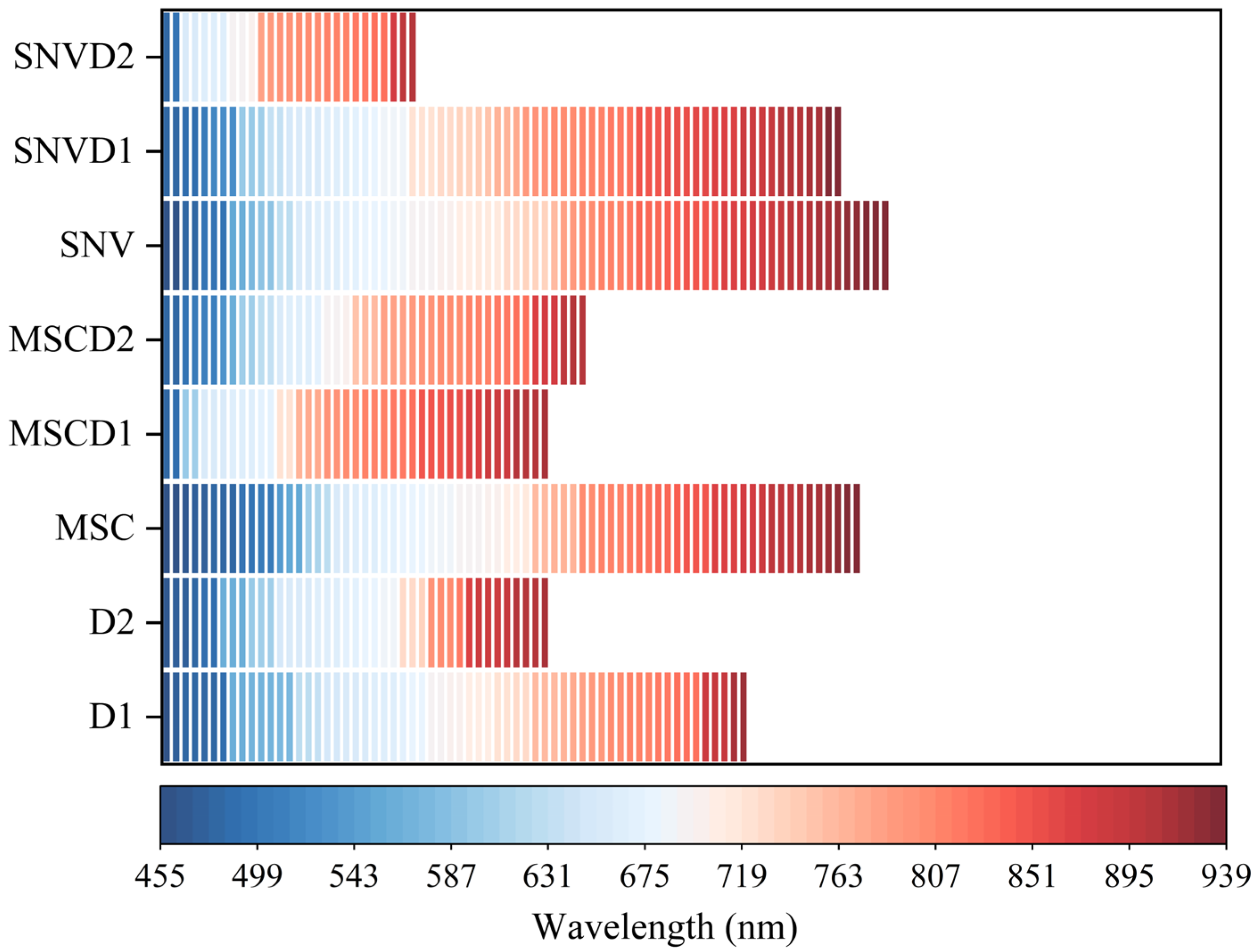
In studies using hyperspectral imaging to estimate soil TOC, various regression algorithms have been developed, including PLSR, artificial neural network (ANN), support vector machine (SVM), and random forest (RF) models. Among these, ANN and SVM are suitable for large datasets [39]. When the soil TOC follows a normal distribution, PLSR demonstrates higher accuracy than RF [40]. PLSR is frequently regarded as the preferred method for quantifying the physicochemical properties of soil and lake sediments from spectral reflectance owing to its excellent stability and accuracy [41,42]. It is an efficient multivariate statistical method that reduces data dimensionality by projecting variable factors onto potential orthogonal components. This method is suitable for variable factors with high covariance, particularly when the experimental sample size is limited, making it widely applicable for quantitative spectral analysis. Consequently, this method was applied to the inversion of TOC in lake sediments.

In this study, we established a relationship between TOC in lake sediments and VNIR spectral data based on the PLSR model, and the model performance was evaluated using correlation coefficients (R) and the root-mean-square error (RMSE). R_c and R_p represent the correlation coefficients of the calibration and validation sets, respectively. All the statistical analysis was conducted in MATLAB software (R2023a), specifically utilizing the “Hyperspectral_Imaging_Sediment_Core-main” on GitHub (https://doi.org/10.5281/zenodo.5764882) (accessed on 24 November 2023) [43].

$$R=\sqrt{1-{\displaystyle \frac{{\sum }_{i=1}^n{\left(y_i-\widehat{y_i}\right)}^2}{{\sum }_{i=1}^n{\left(y_i-\overline{y_i}\right)}^2}}}$$

(1)

$$RMSE=\sqrt{{\displaystyle \frac{{\sum }_{i=1}^n{\left(y_i-\widehat{y_i}\right)}^2}{n}}}$$

(2)

where n denotes the number of samples, $y_i$ denotes the i-th measurement, $\widehat{y_i}$ denotes the i-th estimated value, and $\overline{y_i}$ denotes the average measurement. High R-values and low RMSE-values indicate a significant linear relationship between the model estimations and actual measurements.

2.7. Band Selection

Hyperspectral data contain multiple bands and covariances between neighboring bands. To reduce the workload and complexity of the model, we selected the optimal spectral subset among the original full bands, which could also enhance the model accuracy and simplify mechanism interpretation. The successive projection algorithm, uninformative variable elimination, competitive adaptive reweighted sampling, random forest, particle swarm optimization, variable importance, and GA are common methods for spectral variable selection [44,45,46,47]. This study chose the GA, as it is an efficient multi-band optimization method in analytical spectroscopy, which can significantly improve the estimation accuracy of the model. In addition, a combination of GA and PLSR is frequently used to estimate the physicochemical properties of soils [48].

The GA simulates the natural selection process to select the least number of bands that are highly correlated with the TOC among the original full bands, thereby constituting the optimal spectral subset [49,50]. The GAPLSOPT procedure was initially employed to verify the applicability of the GA and to optimize the number of evaluations. Subsequently, the GAPLS program was used for general variable selection, whereas the GAPLSSP program was specifically designed to optimize the selection of variable subsets for the spectral data. PLOTONE and PLOTMORE programs were used to plot graphs of the selected variables in the final step.

2.8. Sediment Chronology and Time Series Analysis

We used the established high-precision chronological framework of core 12GQ from Wudalianchi Crater Lake [28] to obtain the chronological framework of sediment core GQ2016. The corresponding points at different depths in the two cores can be identified by analyzing the peaks and valleys of the CIE L* time series. These corresponding points were used to establish a depth transformation relationship between the two cores, and the ¹⁴C ages from core 12GQ were transferred to equivalent depths in core GQ2016. The IntCal20 calibration curve [51] from CALIB 8.20 [52] was used to calibrate all ¹⁴C ages of core 12GQ to the calendar age. Then, the Bayesian age-depth model software BACON (Version 2.2) in the R programming package was used to establish an age-depth model (based on terrestrial plant remains) for the sediment cores [53].

The wavelet transform, a time–frequency multi-resolution analytical method [54], enables local signal refinement. Unlike the traditional Fourier transform used in spectral analysis, the wavelet transform can uncover cyclical patterns embedded within a time series, thereby extracting signals across various time scales. In this study, the negative values caused by hyperspectral noise points and dry lake sediments were eliminated, and a wavelet transform was subsequently employed to denoise the reconstructed TOC sequence.

Variations in any time series encompass the superposition of regular waves with different frequencies and intensities [55]. By decomposing the time series into constituent waves characterized by distinct frequencies and comparing the variance magnitudes of these harmonics, the predominant frequency or cycles of the time series fluctuation can be identified. In this study, a power spectrum analysis was conducted using the multi-taper method (MTM) [56,57] implemented in Acycle 2.6.0 software, which is built on MATLAB [58].

3. Results and Discussion

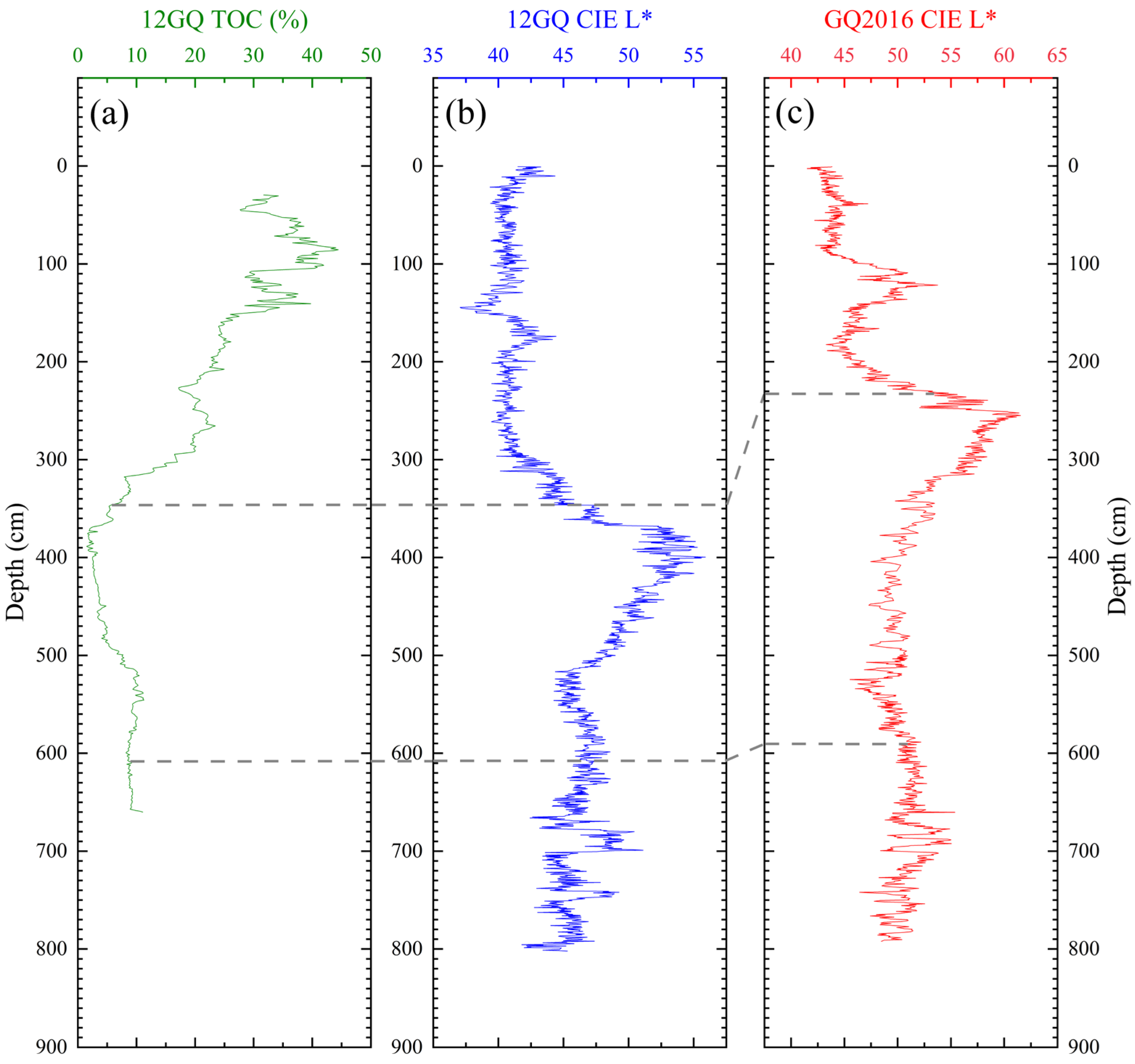
3.1. Chronology

Parallel cores 12GQ and GQ2016 exhibited similar depositional characteristics. Therefore, the distributions of TOC and CIE L* in the two cores were comparable, and the peaks and valleys were visually correlated (Figure 2). Based on the chronology framework of core 12GQ, the age of core GQ2016 at the depth range 232.54–587.80 cm is 38–13 ka BP.

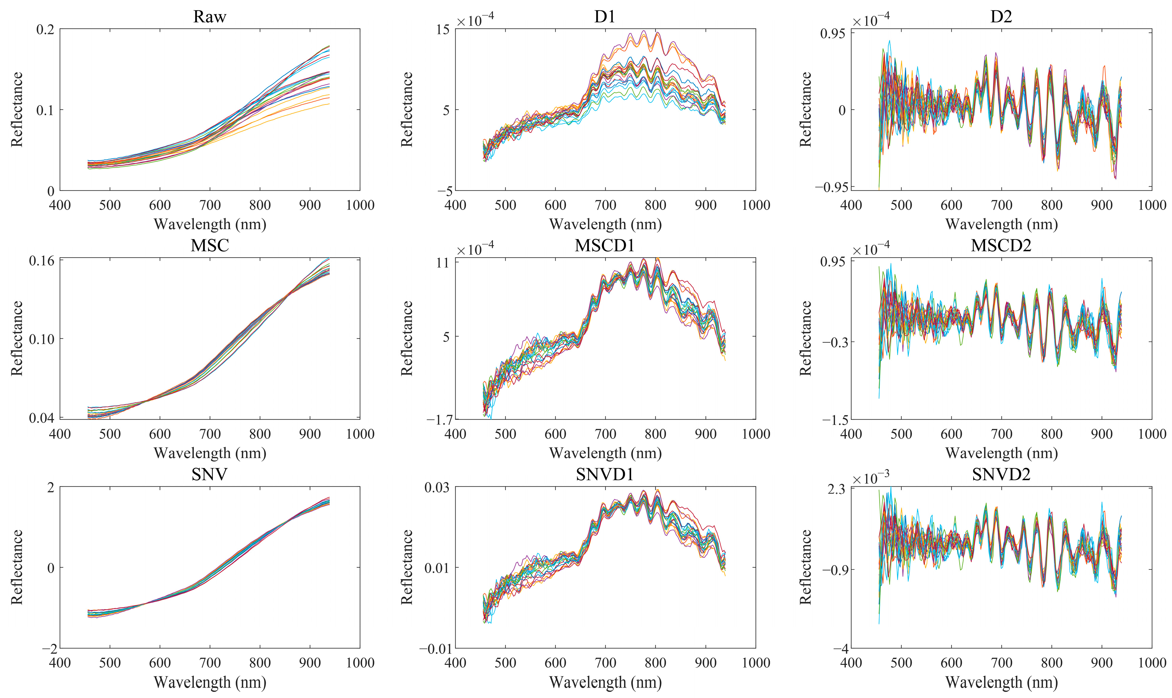
3.2. Spectral Characterization and Preprocessing Results

The spectral curves of these 260 measurement samples were preprocessed and preliminarily analyzed, and 20 typical samples were selected for the spectral curves (Figure 3). The results demonstrated a consistent upward trend with increasing wavelength. After applying SNV and MSC, the spectral curves showed prominent absorption features at 560–580 nm and 860–880 nm. Compared with the spectral curves after D1 processing, the spectral absorption features after D2 processing were more obvious, especially in the range of 600–800 nm, which reduced the overlap and autocorrelation within the bands, thereby enhancing the variability in the spectral data. The composite preprocessing methods of SNVD1 and MSCD1 significantly intensified the absorption features of the D1 spectral curves in the range of 700–900 nm. In contrast, SNVD2 and MSCD2 did not improve the absorption features of the D2 spectral curves.

3.3. Estimation Model of TOC

Based on the GA, 41, 62, 74, 41, 45, 77, 72, and 27 bands were selected to form the optimal spectral subsets for the preprocessing methods D1, D2, MSC, MSCD1, MSCD2, SNV, SNVD1, and SNVD2, respectively (Figure 4). The variability in the optimization of different preprocessing methods for spectral features arises primarily from their distinct sensitivities to these features. These bands were mainly concentrated in the ranges 650–730 nm and 760–910 nm, whereas bands in the 455–480 nm, 510–560 nm, and 730–760 nm ranges were rarely selected, which may be related to the properties of the chemical bonds and their spectral absorption characteristics [59].

To determine the most effective preprocessing method, the eight aforementioned spectral subsets were applied to the PLSR model. The results revealed that model performance was influenced by the preprocessing method employed (

Table 3. Performance of optimal spectral subsets for various preprocessing methods in the PLSR model.

	D1	D2	MSC	MSCD1	MSCD2	SNV	SNVD1	SNVD2
Calibration set R	0.95	0.95	0.94	0.93	0.94	0.90	0.92	0.93
Validation set R	0.93	0.94	0.93	0.92	0.92	0.90	0.92	0.92
Validation set RMSE (%)	1.09	0.99	1.14	1.14	1.10	1.27	1.21	1.16

). The calibration sets for D1 and D2 exhibited higher R-values than the others, which had an R-value of 0.95, indicating its significant ability to fit the training data. The validation sets D1, D2, MSC, and SNVD1 had high R-values, with D2 demonstrating the highest R-value of 0.94 and the lowest RMSE (0.99%). Therefore, D2 was selected for preprocessing the spectral data.

Based on the D2 and GA, the optimal spectral subset with 62 spectral bands was selected, and their correlations with TOC were further analyzed (Figure 5). Bands within the range of 656–669 nm showed significant positive correlations with TOC, with all correlation coefficients exceeding 0.55 (p < 0.01), demonstrating their sensitivity for the estimation of TOC. In particular, the correlation of the 667 nm band with TOC was the highest (0.83). This might be influenced by carbon–iron oxide interactions, such as hematite and acicular iron ore [60], or associated with chemical bonds, including C-H, N-H, C-O, C=O, O-H, and Al-OH [61], which contribute to the distinct spectral absorption features. In addition, bands in the ranges of 578–634 nm, 726–756 nm, and 806–817 nm displayed strong negative correlations below −0.40 (p < 0.01) with TOC. Other studies have also indicated significant correlations between 500 and 800 nm bands and soil TOC, highlighting their potential to estimate TOC [62,63,64].

Therefore, the PLSR model was constructed using the 62 bands preprocessed with D2, selected by the GA, and compared with the PLSR model built with raw data (Figure 6). The R-value of the PLSR model calibration set increased from 0.82 to 0.95, whereas the RMSE decreased from 1.39% to 0.91%. Similarly, the R-value of the validation set increased from 0.75 to 0.94, whereas RMSE decreased from 1.49% to 0.94%. Both the calibration and validation set exhibited R-values above 0.90, indicating that the PLSR model constructed in this study had a high estimation accuracy. In addition, the reduced RMSE further confirmed the reliability of this model. Compared with the SWIR spectra commonly used in previous studies [65], the VNIR spectra used in this study provide more detailed chemical information for reconstructing TOC sequences. Furthermore, the PLSR model was constructed using the average of the spectral sampling regions rather than by randomly selecting the regions of interest [22], which can more accurately reflect the representative characteristics of the samples, thereby enhancing the reliability of the model. With these advantages, TOC variations in core GQ2016 were estimated based on the constructed PLSR model.

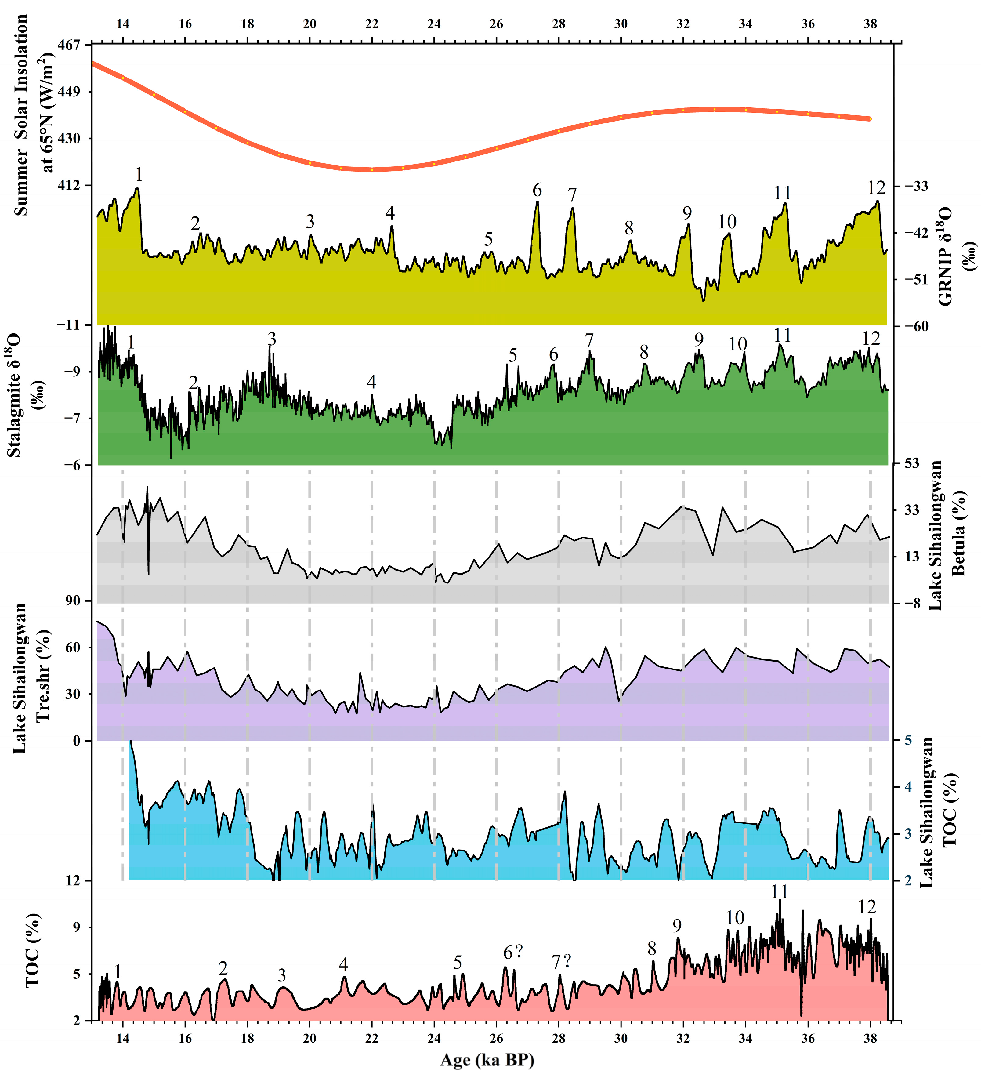
3.4. The Reconstruction of TOC Using the PLSR Model and Its Comparison with the Global Paleoclimate Records

Within the 350–200 cm depth interval of the core, TOC varied around 7%; at 200–150 cm, TOC decreased from 7% to 4%; and above 150 cm, it stabilized at an average of 2% (Figure 7c), indicating that TOC decreased significantly as the depth decreased. A comparison with the RGB image (Figure 7a) revealed that the TOC was lower in the darker layers and vice versa. Meanwhile, the TOC content increased as the reflectance increased (Figure 7b). This phenomenon may be attributed to the balance between the absorption and scattering effects of the TOC. As TOC increases, the concomitant rise in reflectance values, as the scattering effect surpasses the absorption effect, manifests as brighter layers in the RGB image.

Given that the high-resolution TOC data reconstructed using the PLSR model showed significant millennial-scale fluctuations, further power spectral analysis was conducted (Figure 8). The results indicate significant quasi-periodic signals at ~8.7, 4.6, 3.7, 2.9, 2–1, 0.7, 0.4, 0.3, and 0.2 ka during the 38–13 ka BP period, all of which exceed the 99.9% confidence threshold. The ~8.7 ka cycle is generally consistent with the half-precession cycle [66], potentially reflecting low-latitude processes (e.g., summer monsoon), while the ~2–1 ka cycle corresponds to the quasi-periodic signature of the Dansgaard–Oeschger (DO) cycle during glacial periods [67], which is likely to be a high-latitude signal.

To further explore the correlation between the model-reconstructed TOC record and solar radiation, as well as the millennial events during the last glacial period, we compared it with the 65° N summer solar radiation curve [68], the Lake Sihailongwan pollen and TOC records [69], the Greenland ice-core δ¹⁸O record [70], and the Asian stalagmite δ¹⁸O record (Figure 9) [71,72]. The TOC record of the Wudalianchi Crater Lake, reconstructed based on the PLSR model, showed a higher concentration during 38–30 ka BP, followed by a significant decreasing trend from 30 to 20 ka BP, reaching its lowest point during 20–15 ka BP, before gradually increasing. This trend was similar to that of the 65° N summer solar radiation. On the millennial scale, the PLSR-constructed TOC record of this study aligned closely with fluctuations in TOC and pollen of Lake Sihailongwan, Greenland ice core δ¹⁸O, and East Asian stalagmite δ¹⁸O records, which indicate that TOC responds to the millennial-scale events during the last glacial period. These results show the ability of the PLSR model to capture major trends and millennial-scale fluctuations in the TOC records. It is essential to reconstruct high-resolution changes in lake sediments, which is crucial for understanding high-resolution climate change and carbon burial in lakes.

Despite these advantages, the current hyperspectral scanning techniques have several limitations. For instance, there were significant discrepancies between the model estimates and experimental data, particularly in the core ranges of 0–20 cm and 300–350 cm. This may originate from errors in scanning the edge cores with hyperspectral lenses, which generate various noises that affect the spectral data. Several factors may influence the spectral reflectance in addition to the primary variables. These include the moisture content of lake sediments, which affects the absorption of spectral bands; oxidation states, which can alter the color and composition of sediment surfaces; surface flatness, which impacts the optical path of light at different positions; and environmental brightness, which may introduce extraneous light into the spectrometer and interfere with accurate spectral measurements. These factors may compromise the data collected using the hyperspectral scanning technique, ultimately affecting the accuracy and reliability of the analysis results.

Nevertheless, the findings of this study suggest that the hyperspectral scanning technique has considerable value for sediment core analysis. We overcame the limitations of traditional sampling intervals by developing an efficient and convenient sampling and analysis workflow, which significantly improved work efficiency and reduced labor and time costs [73]. Leveraging this advantage, we reconstructed a high-resolution TOC record of sediments from the Wudalianchi crater lake during the period of 38–13 ka BP, which showed significant millennial-scale and short-term extreme events. This provides a more precise record for studying paleoclimatic changes in northeast China [74]. The millennial-scale fluctuation events in the TOC record are consistent with other paleoclimatic records, indicating a close connection between regional climate change and the global climate system. This consistency provides an important basis for further exploration of the response and adaptation mechanisms of these events to climate change. Additionally, by studying these millennial-scale fluctuation events, we can further our understanding of climate systems, which may benefit the comprehension of modern climate change.

4. Conclusions

We employed VNIR hyperspectral imaging, combined with geochemical analytical methods and the PLSR model, to reconstruct the TOC content in the sediment core of Wudalianchi Crater Lake. This method can quantify the TOC in lake sediments with high precision, which is instrumental in understanding millennial-scale climate change patterns and their impacts on lake ecosystems. We successfully reconstructed a high-resolution TOC record of the Wudalianchi Crater Lake sediments from 38 to 13 ka BP. This record aligns well with the millennial-scale events in the summer solar radiation at 65° N, pollen and TOC data from Lake Sihailongwan, the δ¹⁸O record of Greenland ice cores, and the δ¹⁸O records from Asian stalagmites, highlighting the significance of our research in understanding long-term climate dynamics and their ecological implications, which is essential for understanding climate change as well as carbon burial in lakes.

References

1. Jiang, S.W.; Zhou, X.; Li, Z.B.; Tu, L.Y.; Chen, A.Z.; Liu, X.Q.; Ding, M.; Zhang, G.C. Increased effective radiative forcing enhanced the modulating effect of Pacific Decadal Oscillation on late Little Ice Age precipitation in the Jiang-Huai region, China. Clim. Dyn. 2023, 61, 4173–4183. [Google Scholar] [CrossRef]
2. Larocque-Tobler, I.; Filipiak, J.; Tylmann, W.; Bonk, A.; Grosjean, M. Comparison between chironomid-inferred mean-August temperature from varved Lake Zabinskie (Poland) and instrumental data since 1896 AD. Quat. Sci. Rev. 2015, 111, 35–50. [Google Scholar] [CrossRef]
3. Randsalu-Wendrup, L.; Conley, D.J.; Carstensen, J.; Snowball, I.; Jessen, C.; Fritz, S.C. Ecological Regime Shifts in Lake Kalksjon, Sweden, in Response to Abrupt Climate Change Around the 8.2 ka Cooling Event. Ecosystems 2012, 15, 1336–1350. [Google Scholar] [CrossRef]
4. Van Daele, M.; Moernaut, J.; Silversmit, G.; Schmidt, S.; Fontijn, K.; Heirman, K.; Vandoorne, W.; De Clercq, M.; Van Acker, J.; Wolff, C.; et al. The 600 yr eruptive history of Villarrica Volcano (Chile) revealed by annually laminated lake sediments. Geol. Soc. Am. Bull. 2014, 126, 481–498. [Google Scholar] [CrossRef]
5. Zhou, X.; Zhan, T.; Tan, N.; Tu, L.Y.; Smol, J.P.; Jiang, S.W.; Zeng, F.M.; Liu, X.Y.; Li, X.Z.; Liu, G.X.; et al. Inconsistent patterns of Holocene rainfall changes at the East Asian monsoon margin compared to the core monsoon region. Quat. Sci. Rev. 2023, 301, 107952. [Google Scholar] [CrossRef]
6. Lian, Z.L.; Jiang, Z.J.; Huang, X.P.; Liu, S.L.; Zhang, J.P.; Wu, Y.C. Labile and recalcitrant sediment organic carbon pools in the Pearl River Estuary, southern China. Sci. Total Environ. 2018, 640–641, 1302–1311. [Google Scholar] [CrossRef]
7. Zhang, Y.; Shen, J.; Feng, J.M.; Li, X.Y.; Liu, H.J.; Wang, X.Z. Composition, distribution, and source of organic carbon in surface sediments of Erhai Lake, China. Sci. Total Environ. 2023, 858, 159983. [Google Scholar] [CrossRef]
8. Gmitrowicz-Iwan, J.; Kusmierz, S.; Ligeza, S.; Pranagal, J.; Szafran, T. The overlooked carbon cache: Unveiling organic carbon storage in small floodplain lake sediments under humid continental climate changes. Ecol. Indic. 2024, 165, 112224. [Google Scholar] [CrossRef]
9. Cao, Y.M.; Peng, J.; Zhou, S.Q.; Chen, X. Impacts of climate warming and atmospheric deposition on recent shifts in chironomid communities in two alpine lakes, eastern China. Environ. Res. 2024, 246, 118133. [Google Scholar] [CrossRef]
10. Valinia, S.; Futter, M.N.; Cosby, B.J.; Rosén, P.; Fölster, J. Simple Models to Estimate Historical and Recent Changes of Total Organic Carbon Concentrations in Lakes. Environ. Sci. Technol. 2015, 49, 386–394. [Google Scholar] [CrossRef] [PubMed]
11. Yuan, Z.J.; Wu, D.; Niu, L.L.; Ma, X.Y.; Li, Y.M.; Hillman, A.L.; Abbott, M.B.; Zhou, A.F. Contrasting ecosystem responses to climatic events and human activity revealed by a sedimentary record from Lake Yilong, southwestern China. Sci. Total Environ. 2021, 783, 146922. [Google Scholar] [CrossRef] [PubMed]
12. Cheng, C.; Hu, T.P.; Liu, W.J.; Mao, Y.; Shi, M.M.; Xu, A.; Su, Y.W.; Li, X.Y.; Xing, X.L.; Qi, S.H. Modern lake sedimentary record of PAHs and OCPs in a typical karst wetland, south China: Response to human activities and environmental changes. Environ. Pollut. 2021, 291, 118173. [Google Scholar] [CrossRef] [PubMed]
13. Lynch, K.L.; Horgan, B.H.; Munakata-Marr, J.; Hanley, J.; Schneider, R.J.; Rey, K.A.; Spear, J.R.; Jackson, W.A.; Ritter, S.M. Near-infrared spectroscopy of lacustrine sediments in the Great Salt Lake Desert: An analog study for Martian paleolake basins. J. Geophys. Res.-Planets 2015, 120, 599–623. [Google Scholar] [CrossRef]
14. Sorrel, P.; Jacq, K.; Van Exem, A.; Escarguel, G.; Dietre, B.; Debret, M.; McGowan, S.; Ducept, J.; Gauthier, E.; Oberhänsli, H. Evidence for centennial-scale Mid-Holocene episodes of hypolimnetic anoxia in a high-altitude lake system from central Tian Shan (Kyrgyzstan). Quat. Sci. Rev. 2021, 252, 106748. [Google Scholar] [CrossRef]
15. Meyer-Jacob, C.; Michelutti, N.; Paterson, A.M.; Monteith, D.; Yang, H.D.; Weckström, J.; Smol, J.P.; Bindler, R. Inferring Past Trends in Lake Water Organic Carbon Concentrations in Northern Lakes Using Sediment Spectroscopy. Environ. Sci. Technol. 2017, 51, 13248–13255. [Google Scholar] [CrossRef]
16. Ghanbari, H.; Antoniades, D. Convolutional neural networks for mapping of lake sediment core particle size using hyperspectral imaging. Int. J. Appl. Earth Obs. Geoinf. 2022, 112, 102906. [Google Scholar] [CrossRef]
17. Ghanbari, H.; Jacques, O.; Adaïmé, M.É.; Gregory-Eaves, I.; Antoniades, D. Remote Sensing of Lake Sediment Core Particle Size Using Hyperspectral Image Analysis. Remote Sens. 2020, 12, 3850. [Google Scholar] [CrossRef]
18. Jacq, K.; Giguet-Covex, C.; Sabatier, P.; Perrette, Y.; Fanget, B.; Coquin, D.; Debret, M.; Arnaud, F. High-resolution grain size distribution of sediment core with hyperspectral imaging. Sediment. Geol. 2019, 393–394, 105536. [Google Scholar] [CrossRef]
19. Zander, P.D.; Zarczynski, M.; Tylmann, W.; Rainford, S.K.; Grosjean, M. Seasonal climate signals preserved in biochemical varves: Insights from novel high-resolution sediment scanning techniques. Clim. Past 2021, 17, 2055–2071. [Google Scholar] [CrossRef]
20. Butz, C.; Grosjean, M.; Fischer, D.; Wunderle, S.; Tylmann, W.; Rein, B. Hyperspectral imaging spectroscopy: A promising method for the biogeochemical analysis of lake sediments. J. Appl. Remote Sens. 2015, 9, 096031. [Google Scholar] [CrossRef]
21. Van Exem, A.; Debret, M.; Copard, Y.; Vannière, B.; Sabatier, P.; Marcotte, S.; Laignel, B.; Reyss, J.-L.; Desmet, M. Hyperspectral core logging for fire reconstruction studies. J. Paleolimnol. 2017, 59, 297–308. [Google Scholar] [CrossRef]
22. Jacq, K.; Perrette, Y.; Fanget, B.; Sabatier, P.; Coquin, D.; Martinez-Lamas, R.; Debret, M.; Arnaud, F. High-resolution prediction of organic matter concentration with hyperspectral imaging on a sediment core. Sci. Total Environ. 2019, 663, 236–244. [Google Scholar] [CrossRef]
23. Aymerich, I.F.; Oliva, M.; Giralt, S.; Martin-Herrero, J. Detection of Tephra Layers in Antarctic Sediment Cores with Hyperspectral Imaging. PLoS ONE 2016, 11, e0146578. [Google Scholar] [CrossRef]
24. Zhou, X.; Sun, L.G.; Zhan, T.; Huang, W.; Zhou, X.Y.; Hao, Q.Z.; Wang, Y.H.; He, X.Q.; Zhao, C.; Zhang, J.; et al. Time-transgressive onset of the Holocene Optimum in the East Asian monsoon region. Earth Planet. Sci. Lett. 2016, 456, 39–46. [Google Scholar] [CrossRef]
25. Chai, R.S.; Cao, H.J.; Huang, Q.Y.; Xie, L.H.; Yang, F.; Yin, H.B. Temporal and environmental factors drive community structure and function of methanotrophs in volcanic forest soils. J. For. Res. 2023, 35, 2. [Google Scholar] [CrossRef]
26. Zhou, X.; Liu, X.Y.; Zhan, T.; Oyebanji, D.B.; Zhang, J.X.; Tu, L.Y.; Jiang, S.W. Low-latitude forcing on 4.2 ka event indicated by records in the Asian monsoon region. Glob. Planet. Change 2024, 235, 104401. [Google Scholar] [CrossRef]
27. Carneiro, L.M.; do Rosário Zucchi, M.; de Jesus, T.B.; da Silva Júnior, J.B.; Hadlich, G.M. δ13C, δ15N and TOC/TN as indicators of the origin of organic matter in sediment samples from the estuary of a tropical river. Mar. Pollut. Bull. 2021, 172, 112857. [Google Scholar] [CrossRef]
28. Jiang, S.W.; Zhou, X.; Zhan, T.; Tu, L.Y.; Liu, X.Y.; Cui, S.K.; Liu, X.Q.; Chen, A.Z.; Zhang, G.C.; Shen, Y.A. Increased radiocarbon age offset of crater lake sediments linked to cool-dry intervals during the past 40,000 yr. Catena 2024, 238, 107881. [Google Scholar] [CrossRef]
29. Dotto, A.C.; Dalmolin, R.S.D.; ten Caten, A.; Grunwald, S. A systematic study on the application of scatter-corrective and spectral-derivative preprocessing for multivariate prediction of soil organic carbon by Vis-NIR spectra. Geoderma 2018, 314, 262–274. [Google Scholar] [CrossRef]
30. Peng, X.T.; Shi, T.Z.; Song, A.H.; Chen, Y.Y.; Gao, W.X. Estimating Soil Organic Carbon Using VIS/NIR Spectroscopy with SVMR and SPA Methods. Remote Sens. 2014, 6, 2699–2717. [Google Scholar] [CrossRef]
31. Qiao, X.X.; Wang, C.; Feng, M.C.; Yang, W.D.; Ding, G.W.; Sun, H.; Liang, Z.Y.; Shi, C.C. Hyperspectral estimation of soil organic matter based on different spectral preprocessing techniques. Spectrosc. Lett. 2017, 50, 156–163. [Google Scholar] [CrossRef]
32. Barnes, R.J.; Dhanoa, M.S.; Lister, S.J. Standard Normal Variate Transformation and De-Trending of near-Infrared Diffuse Reflectance Spectra. Appl. Spectrosc. 1989, 43, 772–777. [Google Scholar] [CrossRef]
33. Geladi, P.; Macdougall, D.; Martens, H. Linearization and Scatter-Correction for near-Infrared Reflectance Spectra of Meat. Appl. Spectrosc. 1985, 39, 491–500. [Google Scholar] [CrossRef]
34. Savitzky, A.; Golay, M.J.E. Smoothing and Differentiation of Data by Simplified Least Squares Procedures. Anal. Chem. 1964, 36, 1627. [Google Scholar] [CrossRef]
35. Jamshidi, B.; Minaei, S.; Mohajerani, E.; Ghassernian, H. Reflectance Vis/NIR spectroscopy for nondestructive taste characterization of Valencia oranges. Comput. Electron. Agric. 2012, 85, 64–69. [Google Scholar] [CrossRef]
36. Sampaio, P.S.; Soares, A.; Castanho, A.; Almeida, A.S.; Oliveira, J.; Brites, C. Optimization of rice amylose determination by NIR-spectroscopy using PLS chemometrics algorithms. Food Chem. 2018, 242, 196–204. [Google Scholar] [CrossRef]
37. Wang, X.; Esquerre, C.; Downey, G.; Henihan, L.; O’Callaghan, D.; O’Donnell, C. Development of chemometric models using Vis-NIR and Raman spectral data fusion for assessment of infant formula storage temperature and time. Innov. Food Sci. Emerg. Technol. 2021, 67, 102551. [Google Scholar] [CrossRef]
38. Chen, Y.; Deng, J.; Wang, Y.X.; Liu, B.P.; Ding, J.; Mao, X.J.; Zhang, J.; Hu, H.T.; Li, J. Study on discrimination of white tea and albino tea based on near-infrared spectroscopy and chemometrics. J. Sci. Food Agric. 2014, 94, 1026–1033. [Google Scholar] [CrossRef]
39. Kuang, B.Y.; Tekin, Y.; Mouazen, A.M. Comparison between artificial neural network and partial least squares for on-line visible and near infrared spectroscopy measurement of soil organic carbon, pH and clay content. Soil Tillage Res. 2015, 146, 243–252. [Google Scholar] [CrossRef]
40. Knox, N.M.; Grunwald, S.; McDowell, M.L.; Bruland, G.L.; Myers, D.B.; Harris, W.G. Modelling soil carbon fractions with visible near-infrared (VNIR) and mid-infrared (MIR) spectroscopy. Geoderma 2015, 239, 229–239. [Google Scholar] [CrossRef]
41. Gomez, C.; Coulouma, G. Importance of the spatial extent for using soil properties estimated by laboratory VNIR/SWIR spectroscopy: Examples of the clay and calcium carbonate content. Geoderma 2018, 330, 244–253. [Google Scholar] [CrossRef]
42. Stevens, A.; Udelhoven, T.; Denis, A.; Tychon, B.; Lioy, R.; Hoffmann, L.; van Wesemael, B. Measuring soil organic carbon in croplands at regional scale using airborne imaging spectroscopy. Geoderma 2010, 158, 32–45. [Google Scholar] [CrossRef]
43. Jacq, K.; Debret, M.; Fanget, B.; Coquin, D.; Sabatier, P.; Pignol, C.; Arnaud, F.; Perrette, Y. Theoretical Principles and Perspectives of Hyperspectral Imaging Applied to Sediment Core Analysis. Quaternary 2022, 5, 28. [Google Scholar] [CrossRef]
44. Sawant, S.; Manoharan, P. Hyperspectral band selection based on metaheuristic optimization approach. Infrared Phys. Technol. 2020, 107, 103295. [Google Scholar] [CrossRef]
45. Yang, P.M.; Hu, J.; Hu, B.F.; Luo, D.F.; Peng, J. Estimating Soil Organic Matter Content in Desert Areas Using In Situ Hyperspectral Data and Feature Variable Selection Algorithms in Southern Xinjiang, China. Remote Sens. 2022, 14, 5221. [Google Scholar] [CrossRef]
46. Barman, B.; Patra, S. Variable precision rough set based unsupervised band selection technique for hyperspectral image classification. Knowl.-Based Syst. 2020, 193, 105414. [Google Scholar] [CrossRef]
47. Lin, Y.K.; Gao, J.X.; Tu, Y.J.; Zhang, Y.X.; Gao, J. Estimating low concentration heavy metals in water through hyperspectral analysis and genetic algorithm-partial least squares regression. Sci. Total Environ. 2024, 916, 170225. [Google Scholar] [CrossRef]
48. Bao, Y.L.; Meng, X.T.; Ustin, S.; Wang, X.; Zhang, X.L.; Liu, H.J.; Tang, H.T. Vis-SWIR spectral prediction model for soil organic matter with different grouping strategies. Catena 2020, 195, 104703. [Google Scholar] [CrossRef]
49. Leardi, R. Application of genetic algorithm-PLS for feature selection in spectral data sets. J. Chemom. 2000, 14, 643–655. [Google Scholar] [CrossRef]
50. Leardi, R.; Gonzalez, A.L. Genetic algorithms applied to feature selection in PLS regression: How and when to use them. Chemom. Intell. Lab. Syst. 1998, 41, 195–207. [Google Scholar] [CrossRef]
51. Reimer, P.J.; Austin, W.E.N.; Bard, E.; Bayliss, A.; Blackwell, P.G.; Bronk Ramsey, C.; Butzin, M.; Cheng, H.; Edwards, R.L.; Friedrich, M.; et al. The IntCal20 Northern Hemisphere Radiocarbon Age Calibration Curve (0–55 cal kBP). Radiocarbon 2020, 62, 725–757. [Google Scholar] [CrossRef]
52. Stuiver, M.; Reimer, P.J. Extended 14C Data Base and Revised CALIB 3.0 14C Age Calibration Program. Radiocarbon 1993, 35, 215–230. [Google Scholar] [CrossRef]
53. Maarten, B.; Christen, J.A. Flexible paleoclimate age-depth models using an autoregressive gamma process. Bayesian Anal. 2011, 6, 457–474. [Google Scholar] [CrossRef]
54. Morlet, J.; Arens, G.; Fourgeau, E.; Giard, D. Wave-Propagation and Sampling Theory 1. Complex Signal and Scattering in Multilayered Media. Geophysics 1982, 47, 203–221. [Google Scholar] [CrossRef]
55. Mann, M.E.; Lees, J.M. Robust estimation of background noise and signal detection in climatic time series. Clim. Change 1996, 33, 409–445. [Google Scholar] [CrossRef]
56. Vaughan, S.; Bailey, R.J.; Smith, D.G. Detecting cycles in stratigraphic data: Spectral analysis in the presence of red noise. Paleoceanography 2011, 26. [Google Scholar] [CrossRef]
57. Thomson, D.J. Spectrum estimation and harmonic analysis. Proc. IEEE 1982, 70, 1055–1096. [Google Scholar] [CrossRef]
58. Li, M.S.; Hinnov, L.; Kump, L. Acycle: Time-series analysis software for paleoclimate research and education. Comput. Geosci. 2019, 127, 12–22. [Google Scholar] [CrossRef]
59. Galvão, L.S.; Vitorello, Í. Variability of Laboratory Measured Soil Lines of Soils from Southeastern Brazil. Remote Sens. Environ. 1998, 63, 166–181. [Google Scholar] [CrossRef]
60. Jia, N.; Li, L.; Guo, H.; Xie, M.Y. Important role of Fe oxides in global soil carbon stabilization and stocks. Nat. Commun. 2024, 15, 10318. [Google Scholar] [CrossRef]
61. Rossel, R.A.V.; Behrens, T. Using data mining to model and interpret soil diffuse reflectance spectra. Geoderma 2010, 158, 46–54. [Google Scholar] [CrossRef]
62. Guo, L.; Sun, X.R.; Fu, P.; Shi, T.Z.; Dang, L.N.; Chen, Y.Y.; Linderman, M.; Zhang, G.L.; Zhang, Y.; Jiang, Q.H.; et al. Mapping soil organic carbon stock by hyperspectral and time-series multispectral remote sensing images in low-relief agricultural areas. Geoderma 2021, 398, 115118. [Google Scholar] [CrossRef]
63. Meng, X.T.; Bao, Y.L.; Liu, J.G.; Liu, H.J.; Zhang, X.L.; Zhang, Y.; Wang, P.; Tang, H.T.; Kong, F.C. Regional soil organic carbon prediction model based on a discrete wavelet analysis of hyperspectral satellite data. Int. J. Appl. Earth Obs. Geoinf. 2020, 89, 102111. [Google Scholar] [CrossRef]
64. Sun, W.C.; Liu, S.; Zhang, X.; Li, Y. Estimation of soil organic matter content using selected spectral subset of hyperspectral data. Geoderma 2022, 409, 115653. [Google Scholar] [CrossRef]
65. Sola, I.; González-Audícana, M.; Álvarez-Mozos, J. Validation of a Simplified Model to Generate Multispectral Synthetic Images. Remote Sens. 2015, 7, 2942–2951. [Google Scholar] [CrossRef]
66. Jian, Z.M.; Wang, Y.; Dang, H.W.; Lea, D.W.; Liu, Z.Y.; Jin, H.Y.; Yin, Y.Q. Half-precessional cycle of thermocline temperature in the western equatorial Pacific and its bihemispheric dynamics. Proc. Natl. Acad. Sci. USA 2020, 117, 7044–7051. [Google Scholar] [CrossRef] [PubMed]
67. Braun, H.; Christl, M.; Rahmstorf, S.; Ganopolski, A.; Mangini, A.; Kubatzki, C.; Roth, K.; Kromer, B. Possible solar origin of the 1,470-year glacial climate cycle demonstrated in a coupled model. Nature 2005, 438, 208–211. [Google Scholar] [CrossRef]
68. Berger, A.; Loutre, M.F. Insolation values for the climate of the last 10 million years. Quat. Sci. Rev. 1991, 10, 297–317. [Google Scholar] [CrossRef]
69. Mingram, J.; Stebich, M.; Schettler, G.; Hu, Y.Q.; Rioual, P.; Nowaczyk, N.; Dulski, P.; You, H.T.; Opitz, S.; Liu, Q.; et al. Millennial-scale East Asian monsoon variability of the last glacial deduced from annually laminated sediments from Lake Sihailongwan, NE China. Quat. Sci. Rev. 2018, 201, 57–76. [Google Scholar] [CrossRef]
70. Rasmussen, S.O.; Andersen, K.K.; Svensson, A.M.; Steffensen, J.P.; Vinther, B.M.; Clausen, H.B.; Siggaard-Andersen, M.L.; Johnsen, S.J.; Larsen, L.B.; Dahl-Jensen, D.; et al. A new Greenland ice core chronology for the last glacial termination. J. Geophys. Res.-Atmos. 2006, 111, D06102. [Google Scholar] [CrossRef]
71. Dykoski, C.A.; Edwards, R.L.; Cheng, H.; Yuan, D.X.; Cai, Y.J.; Zhang, M.L.; Lin, Y.S.; Qing, J.M.; An, Z.S.; Revenaugh, J. A high-resolution, absolute-dated Holocene and deglacial Asian monsoon record from Dongge Cave, China. Earth Planet. Sci. Lett. 2005, 233, 71–86. [Google Scholar] [CrossRef]
72. Wang, Y.J.; Cheng, H.; Edwards, R.L.; Kong, X.G.; Shao, X.H.; Chen, S.T.; Wu, J.Y.; Jiang, X.Y.; Wang, X.F.; An, Z.S. Millennial- and orbital-scale changes in the East Asian monsoon over the past 224,000 years. Nature 2008, 451, 1090–1093. [Google Scholar] [CrossRef] [PubMed]
73. Cui, S.K.; Zhou, X.; Tu, L.Y.; Liu, X.Y.; Zhan, T.; Jiang, S.W.; Oyebanji, D.B.; Qiao, Y.S.; Liu, X.Q.; Xue, H.P.; et al. Inconsistent Hydroclimate Responses in Different Parts of the Asian Monsoon Region during Heinrich Stadials. Lithosphere 2022, 2022, 1507045. [Google Scholar] [CrossRef]
74. Liu, X.Y.; Zhou, X.; Zhan, T.; Zhou, X.Y.; Wu, H.B.; Jiang, S.W.; Tu, L.Y.; Oyebanji, D.; Shen, Y.A. Pollen evidence for a wet Younger Dryas in northern NE China. Catena 2023, 220, 106667. [Google Scholar] [CrossRef]
Figure 1. Study area and site locations. (a) Location of Wudalianchi Crater Lake (red dot) and other previous paleoclimate reconstructions mentioned in the present study (yellow dots); (b) Wudalianchi Crater Lake and the sampling site locations; (c) instrumental climate data (1958–2000) from Bei’an Station (48°25′N, 126°50′E), near Wudalianchi Crater Lake (based on Chinese Meteorological Administration).
Remotesensing 17 00706 g001
Figure 2. Comparison of parallel cores 12GQ and GQ2016. (a) TOC series of core 12GQ; (b,c) comparison of the CIE L* series of cores 12GQ and GQ2016 [28].
Remotesensing 17 00706 g002
Figure 3. Raw spectra and eight preprocessing results (different colors represent distinct spectral curves).
Remotesensing 17 00706 g003
Figure 4. Optimal spectral subsets for different preprocessing methods.
Remotesensing 17 00706 g004
Figure 5. Correlation between spectral bands in the optimal spectral subset of D2 and TOC.
Remotesensing 17 00706 g005
Figure 6. Performance of raw spectral data for (a) calibration set and (b) validation set in PLSR model; performance of D2 optimal spectral subset for (c) calibration set and (d) validation set in PLSR model (different circles represent different experimental samples).
Remotesensing 17 00706 g006
Figure 7. (a) RGB image of core GQ2016; (b) spectral reflectance of core GQ2016; and (c) TOC reconstructed by the PLSR model. The millennial-scale fluctuations in the sediment core were identified by applying the wavelet transform to remove the noise and extract the fluctuation characteristics.
Remotesensing 17 00706 g007
Figure 8. Power spectral analysis of TOC time series reconstructed using PLSR model.
Remotesensing 17 00706 g008
Figure 9. Comparison of TOC reconstructed based on the PLSR model (red) with 65° N summer solar radiation (orange line) [68], NGRIP Greenland ice core δ18O record (yellow) [70], stalagmite δ18O records from Dongge Cave and Hulu Cave (green) [71,72], Betula pollen records from Lake Sihailongwan (gray) [69], tree and shrub pollen records from Lake Sihailongwan (purple) [69], and TOC records from Lake Sihailongwan (blue) [69]. The numbers in the figure represent obvious millennium-scale fluctuations.
Remotesensing 17 00706 g009