Estimating and Downscaling ESA-CCI Soil Moisture Using Multi-Source Remote Sensing Images and Stacking-Based Ensemble Learning Algorithms in the Shandian River Basin, China

Abstract

Soil Moisture (SM) plays a crucial role in agricultural production, ecology, and sustainable development. The prevailing resolution of microwave-based SM products is notably coarse, typically spanning from 10 to 50 km, which might prove inadequate for specific applications. In this research, various single-model machine learning algorithms have been employed to study SM downscaling, each with its own limitations. In contrast to existing methodologies, our research introduces a pioneering algorithm that amalgamates diverse individual models into an integrated Stacking framework for the purpose of downscaling SM data within the Shandian River Basin. This basin spans the southern region of Inner Mongolia and the northern area of Hebei province. In this paper, factors exerting a profound influence on SM were comprehensively integrated. Ultimately, the surface variables involved in the downscaling process were determined to be Land Surface Temperature (LST), Normalized Difference Vegetation Index (NDVI), Surface Reflectance (SR), Evapotranspiration (ET), Digital Elevation Model (DEM), slope, aspect, and European Space Agency-Climate Change Initiative (ESA-CCI) product. The goal is to generate a 1 km SM downscaling dataset for a 16-day period. Two distinct models are constructed for the SM downscaling process. In one case, the downscaling is followed by the inversion of SM, while in the other case, the inversion is performed after the downscaling analysis. We also employ the Categorical Features Gradient Boosting (CatBoost) algorithm, a single model, for analytical evaluation in identical circumstances. According to the results, the accuracy of the 1 km SM obtained using the inversion-followed-by-downscaling model is higher. Furthermore, it is observed that the stacking algorithm, which integrates multiple models, outperforms the single-model CatBoost algorithm in terms of accuracy. This suggests that the stacking algorithm can overcome the limitations of a single model and improve prediction accuracy. We compared the predicted SM and ESA-CCI SM; it is evident that the predicted results exhibit a strong correlation with ESA-CCI SM, with a maximum Pearson correlation coefficient (PCC) value of 0.979 and a minimum value of 0.629. The Mean Absolute Error (MAE) values range from 0.002 to 0.005 m³/m³, and the Root Mean Square Error (RMSE) ranges from 0.003 to 0.006 m³/m³. Overall, the results demonstrate that the stacking algorithm based on multi-model integration provides more accurate and consistent retrieval and downscaling of SM.

1. Introduction

Soil Moisture (SM) is crucial for water, heat, and energy exchange in ecosystems and environmental processes. In agriculture, it directly impacts crop growth, yield, and irrigation efficiency. Effective SM management is vital for sustainable agriculture, improving water use efficiency, minimizing waste, and protecting water resources. It supports long-term productivity and contributes to environmental sustainability and climate resilience [1,2,3]. Previously, SM monitoring methods primarily relied on field monitoring. However, the measurement of SM in the field poses challenges and requires significant resources. Furthermore, it is not feasible to monitor SM on a large scale with high frequency in real-time. As remote sensing technology has advanced, an increasing number of studies have incorporated remote sensing techniques into SM prediction research [4,5]. Remote sensing technology not only enables the acquisition of SM data over large areas but also offers various temporal resolutions. Consequently, remote sensing technology has emerged as a primary and crucial approach for SM prediction and monitoring in contemporary times [6,7,8,9]. Microwave technology is widely utilized for acquiring long-term and large-scale SM data. Currently, satellites that can provide SM observations include NASA’s SM Active Passive (SMAP, 2015-present) [10], EASA’s SM and Ocean Salinity (SMOS, 2010-present) [11], EASA’s Advanced SCATterometer (ASCAT, 2007-present) [12], Advanced Microwave Scanning Radiometer-2 (AMSR2, 2012-present) from JAXA [13], FY-3B/C from China [14], and the European Space Agency’s Climate Change Initiative (ESA-CCI, 1978–2021) [15,16,17]. ESA-CCI SM is an extensive temporal dataset that combines satellite data on SM from multiple sensors, including active and passive microwave sensors. It comprises three types of datasets: active, passive, and fused. The spatial resolution of the data is 0.25°, and it provides a temporal resolution of 1 day. ESA CCI SM offers more than 40 years of continuous time series, encompassing positive, negative, and combined data, which are available in different versions. This globally accessible dataset provides valuable insights for various applications, such as agriculture, meteorology, and other fields. This array of passive microwave remote sensing SM products offers the large-scale distribution of SM, thereby furnishing essential basic data for global or large-scale regional studies. It provides vital basic data for global or regional research endeavors [16,18,19,20,21]. Long time-series SM products at a 25 km scale can provide adequate support for specific large-scale studies. This resolution is insufficient to satisfy the requirements for SM resolution in hydrological models and other land-surface evapotranspiration models. Therefore, it is imperative to conduct downscaling research on passive microwave products to acquire SM data with a high spatial resolution. These high-resolution data are of great significance for enhancing the accuracy and applicability of hydrological and land-surface process simulations and can contribute to a more in-depth understanding of the complex interactions within the terrestrial ecosystem [22,23,24,25,26,27]. The acquisition of SM at a fine spatial resolution has emerged as a key research priority.

Also, optical remote sensing is widely utilized in numerous studies on SM inversion. The application of optical data can enhance the integration of SM at higher spatial resolution. NDVI (Normalized Difference Vegetation Index) is closely associated with vegetation density and surface SM since a higher NDVI value indicates the need for increased SM to support vegetation growth. Multiple researchers have employed NDVI to establish various drought indices in order to investigate its correlation with SM [28,29,30]. In numerous academic studies, the Land Surface Temperature (LST) has frequently been employed to construct a triangular feature space alongside the Normalized Difference Vegetation Index (NDVI). This approach facilitates subsequent SM inversion and downscaling investigations [31,32,33,34,35]. ET is an essential factor that significantly influences SM, and there exists a reciprocal relationship between evapotranspiration and SM. The sufficiency of SM impacts evapotranspiration, while the intensity and circumstances of evapotranspiration also influence the content of SM [36]. SM significantly influences reflectance. Specifically, an increase in SM results in higher reflectance of the soil surface, whereas a decrease in SM leads to lower reflectance [37]. DEM can provide essential topographic information such as terrain elevation, mountainous regions, and river networks. Among the various factors affecting SM, topography is recognized as a significant influencing factor. In the field of SM inversion, numerous researchers have explored the integration of DEM with other relevant features [38,39]. In various studies, diverse parameters have been found to play distinct roles. Generally, by incorporating a broader range of relevant characteristics, more precise SM predictions can be obtained.

On the basis of extensive understanding and analysis of research progress in soil moisture remote sensing inversion at home and abroad, soil moisture inversion is roughly divided into three areas: the visible–near-infrared method [40,41,42,43,44], thermal infrared method [45,46,47,48,49] and microwave remote sensing method [50,51,52].

In recent years, continuous progress has been made in the research on the spatial downscaling of passive microwave SM remote sensing products both at home and abroad. In the process of SM downscaling, the selection of methods and the screening of variables have become key factors affecting the results, and they are also important considerations for meeting the requirements of spatio-temporal resolution and accuracy [26,53]. Currently, there are numerous SM downscaling techniques available, including fitting regression methods, approaches based on physical models, data synchronization, and spatial interpolation [54]. With the development of machine learning technology, machine learning algorithms are increasingly being widely used in SM downscaling modeling. Compared with other methods, they can more effectively predict nonlinear correlations [24,27,55,56,57,58,59,60,61,62].

Because of the numerous uncertainties that impact SM, traditional methods may not adequately capture the intricate relationship between each variable and SM under varying uncertainties. Machine learning, however, possesses the capability of internal learning, enabling it to enhance its performance and accuracy progressively. It can effectively simulate the complex nonlinear relationship between target variables and auxiliary parameters, facilitating the prediction of target variables [63,64,65,66,67]. With the advancement of machine learning, various methods have been applied to SM prediction. However, these different models often possess individual limitations and may not fully meet the prediction requirements for data from diverse regions. Our research has identified that the integrated model-stacking algorithm, which combines multiple single models, is a superior approach that can yield improved and more reliable prediction results compared to any singular model [5,29,68,69,70]. The Stacking approach involves constructing multiple types of base learners to generate initial predictions, which are then utilized to train a secondary learner for the final prediction outcomes. The secondary learner is typically a regression model. Therefore, the selection of the base learners is crucial in this process. For our study, we opted for four base learners: RF, LightGBM, XGBoost, and CatBoost. RF performs exceptionally well because even the addition of new data points to the dataset has minimal impact on the overall algorithm. It primarily influences individual decision trees rather than the entire ensemble [71]. However, learning the feature combinations in RF can be challenging. During the generation process of each decision tree, each split is based on a locally optimal choice, and there is no guarantee that the final result will be globally optimal. LightGBM employs a one-sided gradient sampling technique to optimize time and space utilization for computational operations [72]. Nevertheless, the LightGBM algorithm has the potential to grow deeper decision trees, which may lead to overfitting. Additionally, as a bias-based algorithm, it tends to be more susceptible to noise. XGBoost, a powerful machine learning algorithm, possesses excellent scalability and versatility, enabling it to effectively process datasets of varying sizes [73]. In spite of that, XGBoost employs a level-wise strategy for generating decision trees, whereby the leaves at each layer are split simultaneously. This approach facilitates multi-threaded optimization and helps prevent overfitting. However, it is worth noting that several leaf nodes exhibit low splitting gains, rendering further splitting unnecessary. CatBoost showcases impressive proficiency in effectively addressing nonlinearity and high dimensionality, ultimately yielding outputs of exceptional accuracy [74,75]. At the same time, CatBoost possesses a multitude of hyperparameters that require careful adjustment, thus resulting in additional time consumption for parameter tuning.

Currently, when using multi-source remote sensing data for SM estimation and downscaling research, passive microwave technology can provide SM data with higher temporal resolution. However, due to its longer wavelength, it results in lower spatial resolution. At the same time, when using machine learning for SM downscaling modeling, static parameters are typically employed, which may lead to the model being less responsive to SM changes and unable to fully reflect the dynamic variations of SM in both time and space. Therefore, there are some issues regarding the applicability of passive-active microwave fusion SM products in downscaling.

Most existing downscaling models use static parameters and the spatial resolution of long time-series SM products is too low—these problems make it difficult to meet the requirements of hydrological models and other surface models for higher-resolution SM data. In this study, our objective is to develop a robust and accurate framework for downscaling SM using ESA-CCI SM data. We consider various factors that influence SM changes and leverage multiple sources of remote sensing data. First, this study initiated the research on SM downscaling using the continuous active-passive microwave SM product data from ESA-CCI. Second, the established Ada-Stacking algorithm based on multi-model fusion was employed. Meanwhile, two SM downscaling processes grounded in the integrated learning algorithm were constructed. One approach is to resample all the data to a 1 km resolution first and then conduct SM estimation. The other is to perform SM estimation first and then carry out downscaling resampling to a 1 km resolution. The common objective of these two processes is to successfully downscale the 25 km SM products to a 1 km spatial resolution. To validate the robustness of the algorithm, the results of the single-algorithm CatBoost model and the Stacking model under the same steps were compared concurrently. Finally, the differences between the two methods and the potential of the Stacking algorithm in enhancing SM downscaling will be analyzed and discussed in detail.

2. Materials and Methods

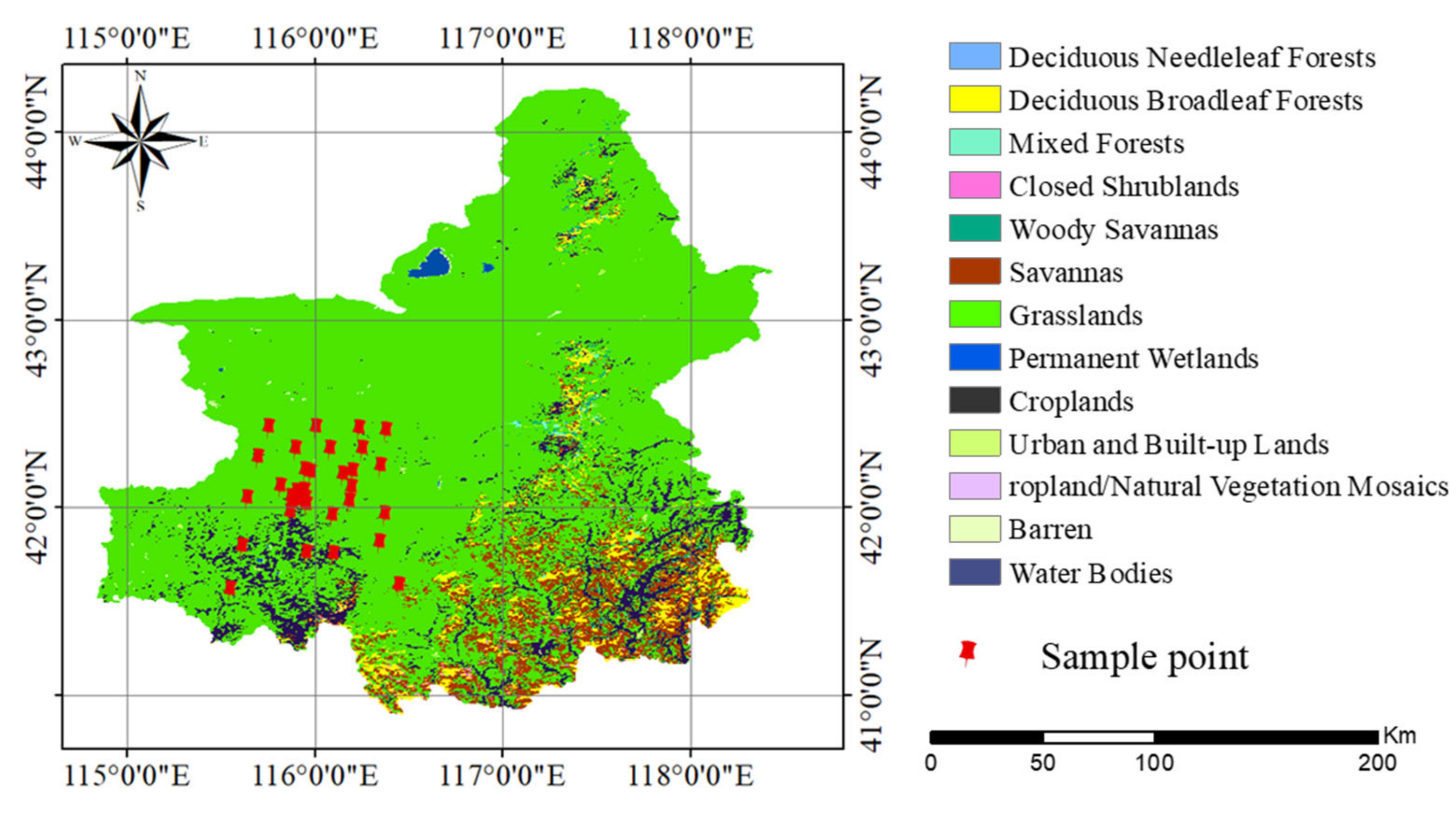
2.1. Study Area

The study areas were situated in the southern part of Inner Mongolia and the northern part of Hebei, encompassing Guyuan County, Longhua County, Fengning Manchu Autonomous Region, Weichang Manchu Autonomous Region, Keshiketeng Banner, Taibu Si Banner, Zhenglan Banner, and Duolun County. The study area spans from 40.89° to 44.23° latitude and from 114.83° to 118.44° longitude. Figure 1 illustrates the land cover of the study area using the MODIS MCD12Q1 product. This region boasts a natural ecological environment abundant in forest and grassland ecosystems, which are rich in biodiversity. It is also characterized by interlacing zones of agriculture, pastoralism, and forestry. These features are of utmost importance when investigating typical regional SM inversion.

2.2. Dataset

2.2.1. MODIS Product Data

Moderate Resolution Imaging Spectroradiometer (MODIS) is a medium-resolution imaging spectrometer consisting of two satellites, Terra and Aqua. This advanced instrument is an integral part of the U.S. Earth Observing System (EOS) program, enabling precise observation of global biological and physical processes. In this study, we utilized various MODIS products available at https://ladsweb.modaps.eosdis.nasa.gov/search/ (accessed on 18 January 2024) as our data sources [76,77]. The MOD09A1 product offers synthetic data with surface reflectance (SR) for bands 1 to 7 at a resolution of 500 m. These data are generated every eight days, providing timely and up-to-date information on the state of the Earth’s surface. Additionally, we employed MOD11A2 data, which represents the Land Surface Temperature (LST) during clear weather conditions over an 8-day period, and has a spatial resolution of 1 km. Furthermore, we utilized MOD13A2 synthetic Normalized Difference Vegetation Index (NDVI) data, which is available at a 16-day temporal resolution and a spatial resolution of 1 km. For evaporation data, we utilized MOD16A2, which provides information at an 8-day resolution of 500 m. Lastly, we incorporated MCD12Q1 data, representing land cover types, with a resolution of 500 m in our analysis. To ensure consistency, we confined our study to MODIS product data acquired between April and September from 2018 to 2020. We resampled all data sources to achieve a consistent spatial resolution of 1 km and 25 km.

2.2.2. SM Data

The ESA’s Climate Change Initiative (CCI) remote sensing SM data consists of an extensive time series that integrates various satellite-derived SM data products. These products encompass active and passive datasets, as well as combined datasets. The utilization of both active and passive microwave sensors enables the product to offer spatial resolutions of 0.25° and temporal resolutions of one day [16,18,19]. For our research, we have chosen version V7.1 of the combined product, which includes the data from April to September between 2018 and 2020. Our objective was to determine the downscaled SM at a resolution of 1 km over a 16-day period using the ESA-CCI SM data. To accomplish this, we extracted the daily ESA-CCI SM value within the 16-day timeframe based on the NDVI time series and then calculated the average SM for that specific period. Moreover, in this study, the bilinear interpolation method is employed to resample the ESA-CCI dataset from its original resolution of 25 km to a finer 1 km scale. As a result, we obtained two sets of SM values: one at 1 km resolution and another at 25 km resolution.

The acquired SM data were obtained from the in situ measurement dataset (2019) of the SM and temperature wireless sensor network within the Shandian River Basin. SM was measured at 34 sites, spanning five different depths (3, 5, 10, 20, and 50 cm). For the purpose of this paper, the SM data specifically at a depth of 3 cm were utilized. The SM values varied between 0 and 0.40 m³/m³ [58,59,60].

2.2.3. ASTER GDEM Data

ASTER GDEM (https://www.gscloud.cn/, accessed on 18 January 2024) is a globally accessible digital elevation data product developed through the collaboration of NASA and the Ministry of Economy, Trade and Industry (METI) of Japan. This dataset provides detailed terrain information at a global scale, featuring a spatial resolution of 30 m. In our study, we employed the merged ASTER GDEM to acquire elevation and slope data, conducting resampling at intervals of both 1 km and 25 km.

Table 1. Satellite datasets used in this study.

Product	Parameters	Spatial Resolution
MOD09A1	SR	500 m/8 days
MOD13A2	NDVI	1 km/16 days
MOD11A2	LST	1 km/8 days
MOD16A2	ET	500 m
MCD12Q1	Land cover type	500 m
ASTER GDEM	Aspect Slope DEM	30 m
ESA-CCI	SM	25 km/daily
MOD09A1	SR	500 m/8 days
MOD13A2	NDVI	1 km/16 days
MOD11A2	LST	1 km/8 days
MOD16A2	ET	500 m
MCD12Q1	Land cover type	500 m

displays the satellite datasets utilized in this research.

2.3. Methods

2.3.1. Data Processing

First, we utilized the MODIS ReProjection Tool (MRT, https://lpdaac.usgs.gov/news/modis-reprojection-tool-version-33-available/, accessed on 18 January 2024) tool provided by the official NASA website to splice and transform MODIS data products. Subsequently, we cropped the data to retrieve all surface variables within our designated study area. Our objective was to obtain SM data at a resolution of 1 km, while the spatial resolution of ESA-CCI SM data is 25 km. Thus, it was necessary to resample all surface parameters (NDVI, LST, SR, and ET) to resolutions of 1 km and 25 km, respectively.

For the inclusion of topographic digital variables in this paper, we selected DEM, Slope, and Aspect. Initially, we employed ArcGIS to generate Slope and Aspect using DEM. These variables were then resampled to resolutions of 1 km and 25 km using the bilinear interpolation method.

Since this paper focused on downscaling, based on the 16-day temporal resolution of ESA-CCI data, we averaged the daily ESA-CCI SM data over a period of 16 days to obtain the 16-day SM data. It is important to note that due to variations in spatial and temporal resolutions, some pixels may contain missing numerical values. However, our 16-day data can partially address these missing values to some extent.

Finally, we will obtain SM products with a 1 km spatial resolution and a 16-day temporal scale.

2.3.2. Stacking Algorithm

Stacking, a widely used ensemble modeling technique in the field of machine learning, aims to enhance prediction quality by combining outputs from multiple weak learners and meta-learners. The process involves using predictions from sub-models as input for an algorithm that learns to effectively combine these inputs for more accurate predictions. Stacking is also known as stacked generalization and can be considered an extension of the Model Averaging Ensemble technique. In stacking, all sub-models contribute equally, based on their performance weights, to construct a new model that generates improved predictions. This new model is then placed atop the existing models, hence the term “stacking” [67,78].

Therefore, in this study, we have selected Random Forest (RF), Light Gradient Boosting Machine (LightGBM), eXtreme Gradient Boosting (XGBoost), and Categorical Features Gradient Boosting (CatBoost) as the first layer meta-learners. Additionally, Linear Regression has been chosen as the second layer meta-learner. The basic architecture of the stacking approach is depicted in Figure 2.

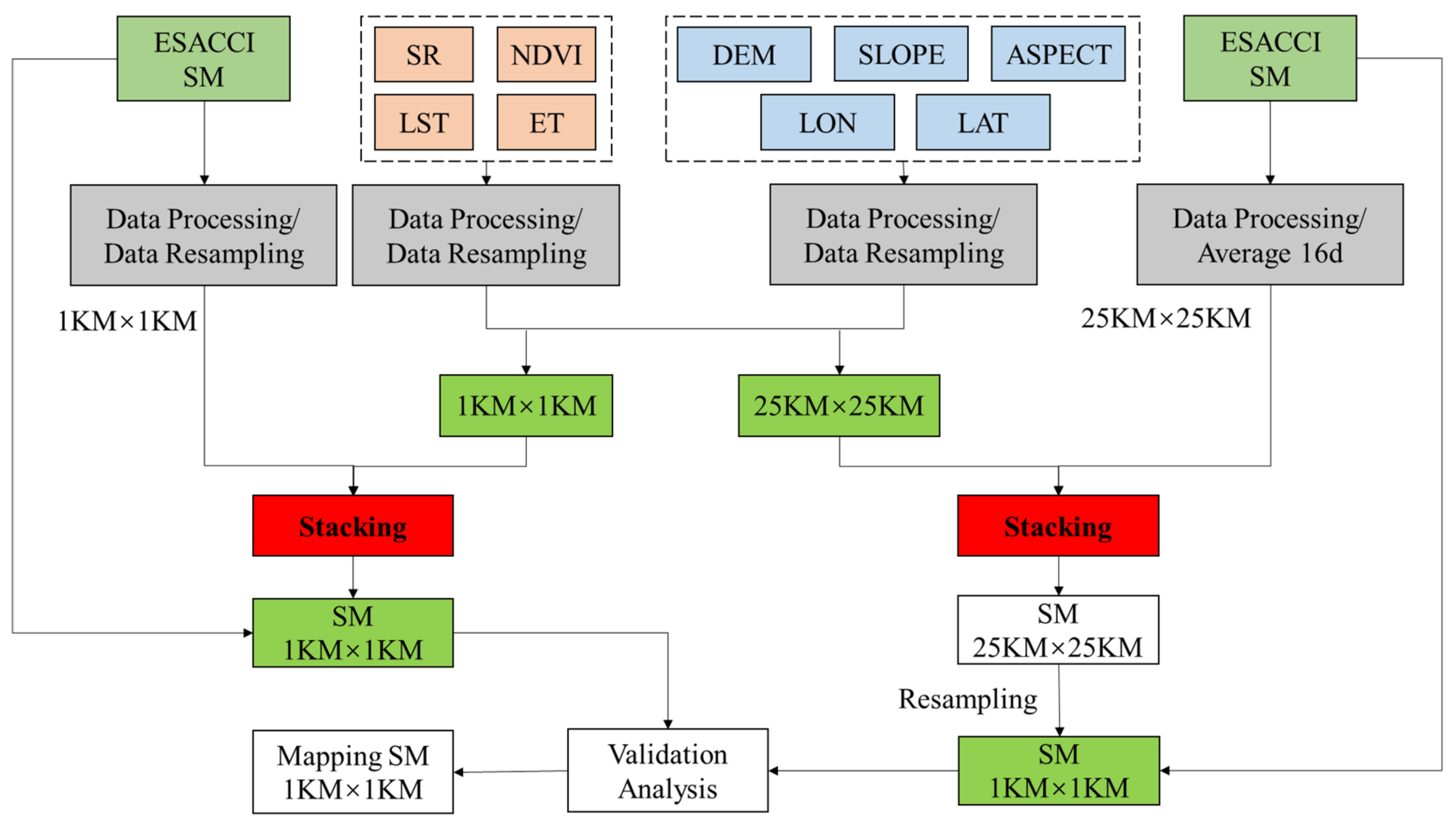
2.3.3. The Overall SM Retrieval Framework

Figure 3 illustrates the comprehensive flowchart of the stacking algorithm used for SM retrieval. Additionally, Figure 4 presents a detailed flowchart outlining the process of SM retrieval and downscaling specifically based on the Stacking algorithm. Our approach involves constructing a two-layer model for integration purposes. The first layer comprises four distinct base learners, namely RF, LightGBM, XGBoost, and CatBoost, which were selected for this study. Each model is utilized to combine forecasts in order to mitigate model bias. In the second layer, linear regression models are employed. The specific steps involved in this process are as follows:

(1)

The dataset, consisting of surface parameters and DEM data, is partitioned into training and prediction data sets. Subsequently, the samples are further divided into K-fold subsets with equal sizes.

(2)

Each base learner is utilized for K-fold training. During each training iteration, K-1 data samples are used as the training set, while the remaining data sample is used for prediction, resulting in K data samples after training. The prediction samples are predicted during each training phase.

(3)

Combine k sets of prediction data to obtain new training sample data, which will serve as the second layer of prediction data.

(4)

Utilize the data acquired in step 3 and input them into the second layer to obtain the ultimate prediction outcome, which provides us with the required SM prediction results.

Figure 3. The overall flowchart of SM retrieval of stacking algorithm.

Figure 3. The overall flowchart of SM retrieval of stacking algorithm.

Figure 4. The detailed flowchart of SM retrieval and downscaling based on the Stacking algorithm.

Figure 4. The detailed flowchart of SM retrieval and downscaling based on the Stacking algorithm.

Within this research, surface parameters such as LST, NDVI, ET, and SR were collected. Additionally, DEM was incorporated as a predictor to account for the impact of topography. The Stacking framework, built upon multiple sources of remote sensing data, can be succinctly divided into two detailed steps outlined below.

The primary stages of downscaling, employing the Stacking algorithm, can be elucidated by considering the following two models:

Model 1: The stacking model integrates all remotely sensed surface parameters, SM products, and measured SM data. However, there are significant differences in spatial and temporal resolution among the data derived from various remote sensing satellites. This introduces uncertainty in the accuracy of SM downscaling. Therefore, our first approach is to resample the coarse-resolution 25 km ESA-CCI SM data to 1 km resolution, as well as the DEM (30 m), ET (500 m), and SR (500 m) data, ensuring consistent spatial resolution across all surface data. Subsequently, the 16-day average data are also resampled to 1 km resolution. The resulting 1 km data set is used to build the Stacking model, with a division into testing and training sets, ultimately producing the downscaled 1 km SM product.

Model 2: In an alternate scenario, we initially resample all surface parameters to a uniform spatial resolution of 25 km, aligning them with ESA-CCI SM. These parameters include NDVI, LST, ET, SR, and DEM. Subsequently, we employ all the 25 km parameters as inputs for the stacking model. To evaluate the performance of the stacking algorithm, we partition the dataset into training and test sets and utilize the K-fold cross-validation method. The stacking algorithm’s effectiveness is verified through this evaluation approach. The outcome of this process yields 25 km SM data, from which we derive the final 1 km downscaled SM product using bilinear interpolation.

Bilinear interpolation is an efficient method in image processing, demonstrating remarkable efficacy in preserving image details and skillfully handling missing pixel values. In terms of detail preservation, it is far more sophisticated than basic interpolation methods. When an image contains fine-grained structures, bilinear interpolation can capture the essence of these features with high precision. By taking into account the four adjacent pixels, it can more accurately simulate the local variation of pixel values. When dealing with missing pixel values, bilinear interpolation provides a robust solution. Instead of simply guessing the missing values, it uses a well-defined weighted average calculation based on the surrounding pixels. In contrast, bilinear interpolation strikes a balance between the two. It minimizes artifacts or distortions by creating a smooth transition between pixels. As a result, the interpolated image looks natural and realistic, showing no obvious signs of the interpolation process. Moreover, bilinear interpolation can reduce discontinuities or singularities during the interpolation process. Through its weighted average approach, it can analyze the local gradient of pixel values and adjust the interpolation accordingly [79,80]. Due to these remarkable advantages, bilinear interpolation is the preferred choice in this article.

The reason for using the stacking algorithm in this study is that the stacking algorithm differs from traditional single-model machine learning SM downscaling methods primarily in the following ways: The stacking algorithm typically integrates multiple different ML models, combining or stacking their prediction results to produce more accurate and stable downscaling outcomes. It leverages the advantages of multiple models, enabling it to capture more complex relationships between SM and related variables. In contrast, traditional single-model machine learning SM downscaling methods rely on a single model, and their performance is limited by the capabilities and assumptions of that model. As a result, the ability to capture complex relationships may be relatively limited, and when faced with varying data characteristics and practical application scenarios, the flexibility and accuracy may not be as high as that of the stacking algorithm.

We also employed the CatBoost algorithm as a single model to perform downscaled SM analysis for both models. The objective was to determine which approach yielded superior results in producing downscaled SM products, the single model or the integrated model.

In this article, we chose Scikit-Learn version 1.6.0. Scikit-Learn, commonly referred to as Sklearn, represents a Python-based machine learning library. Within Sklearn, six principal task-oriented modules encompass classification, regression, clustering, dimensionality reduction, model selection, and preprocessing. In our study, we harnessed the regression capabilities of Sklearn by employing algorithmic modules such as Random Forest (RF), LightGBM, XGBoost, and CatBoost to perform regression tasks.

RF is resistant to overfitting and can evaluate feature importance. LightGBM is characterized by fast speed, low memory consumption, and parallel learning capabilities. XGBoost has strong regularization, excels at handling complex relationships and missing values. CatBoost can automatically handle categorical features, performs well with small-sample data, and offers good stability. By stacking these algorithms, we can integrate different learning perspectives, thereby improving the accuracy of the SM downscaling results, which is why we selected these algorithms to build the stacking algorithm in this study. The advantage of the stacking algorithm lies in its adoption of adaptive adjustment of thresholds and weights, enabling it to automatically adapt to different data characteristics and complex scenarios. Through adaptive adjustment, it can accurately identify these differences and dynamically assign weights and thresholds to each base algorithm (RF, LightGBM, XGBoost, and CatBoost). As data continues to accumulate and be updated, the stacking algorithm can continuously engage in self-learning and optimization.

Among them, the important parameter settings are as follows.

For the Random Forest (RF), we set the value of n_estimators to 10, 20, 50, 100, 200, and 500, and adopted max_features = ‘auto’.

For the LightGBM model, we used boosting_type = ‘gbdt’, objective = ‘regression’, num_leaves = 1200, learning_rate = 0.17, and the values of n_estimators were 110, 220, and 330. The max_depth values were 60, 90, and 100, respectively, metric = ‘rmse’, bagging_fraction = 0.8, feature_fraction = 0.8, and reg_lambda = 0.9.

In the XGBoost model, the values of max_depth were 40, 45, and 50, n_estimators were 30, 50, and 80. We also set silent = True and objective = ‘reg:gamma’.

For CatBoost, the max_depth was set to 20 and 50, n_estimators were 50, 100, and 300, learning_rate = 0.8, and loss_function = ‘RMSE’.

These hyperparameter settings play a crucial role in the model training and evaluation process, helping to improve the prediction performance of the models.

2.3.4. Model Validation and Evaluation

This study utilizes four frequently employed performance metrics for SM retrieval: Bias, Mean Absolute Error (MAE), Root Mean Squared Error (RMSE), and the Pearson Correlation Coefficient (PCC). These metrics can be computed in the following manner:

$$Bias=E\left[{\theta }_{est}\right]-E\left[{\theta }_{true}\right]$$

(1)

$$MAE={\displaystyle \frac{1}{m}}{\displaystyle \sum _{i=1}^m\left|\left({\theta }_{est}-{\theta }_{true}\right)\right|}$$

(2)

$$RMSE=\sqrt{E\left[{\left({\theta }_{est}-{\theta }_{true}\right)}^2\right]}$$

(3)

$$PCC={\displaystyle \frac{E\left[\left({\theta }_{est}-E\left[{\theta }_{est}\right]\right)\left({\theta }_{true}-E\left[{\theta }_{true}\right]\right)\right]}{{\sigma }_{est}{\sigma }_{true}}}$$

(4)

where E [.] is the mean operator, ${\theta }_{true}$ represents the in situ SM or ESA-CCI SM. ${\theta }_{est}$ represents the predicted SM. ${\sigma }_{est}$ and ${\sigma }_{true}$ are the standard deviation of the estimated SM and in situ SM. m is the total amount of data.

3. Results

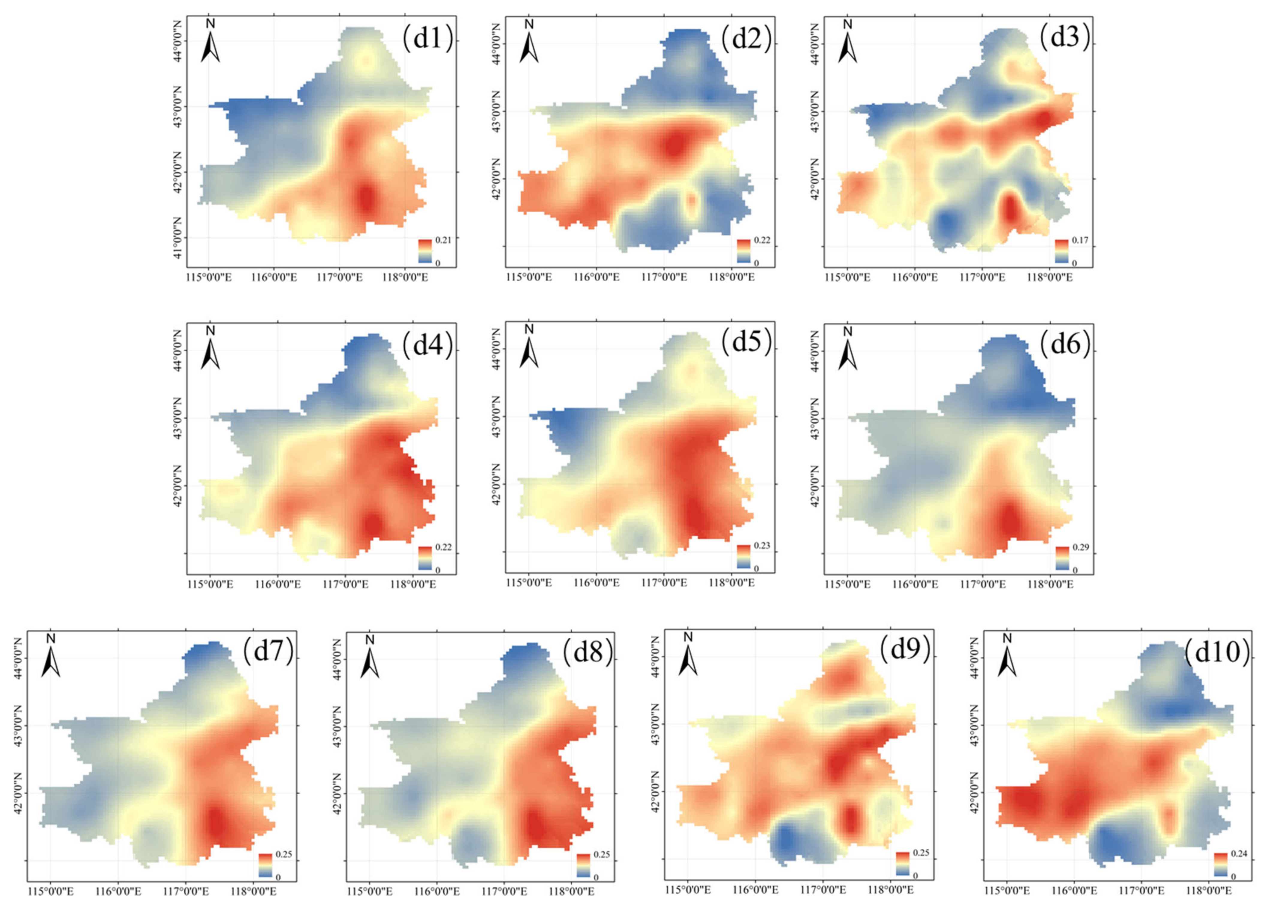
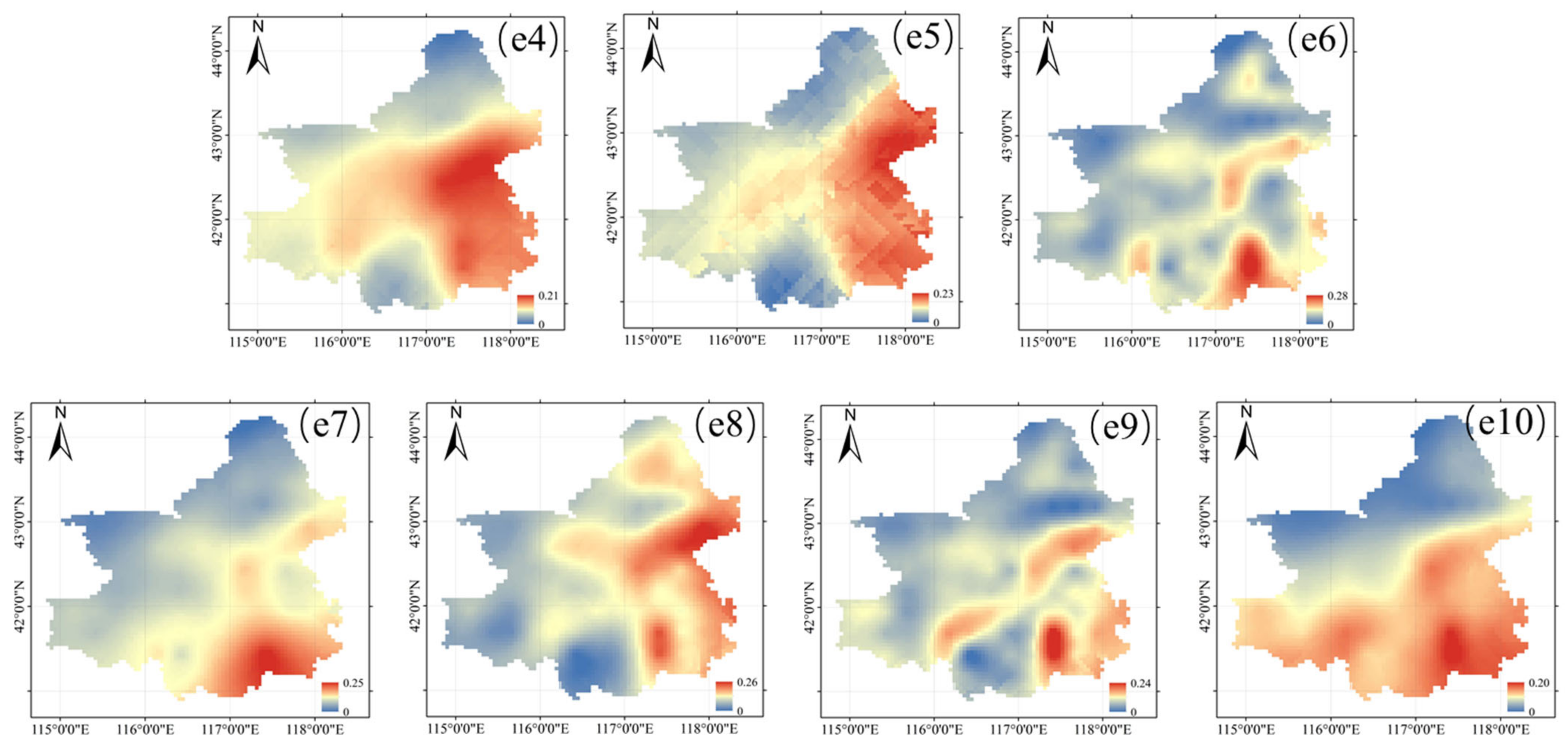
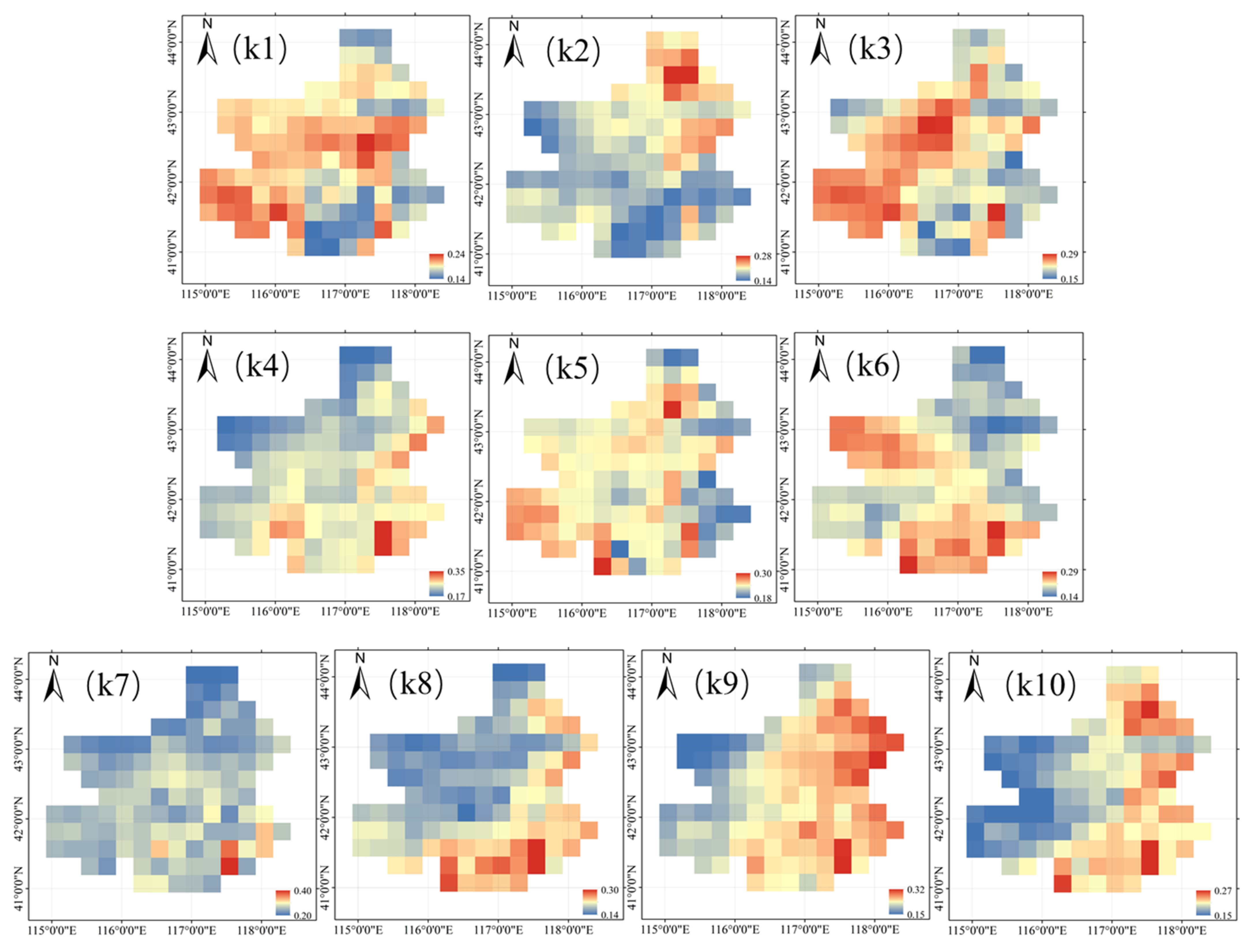
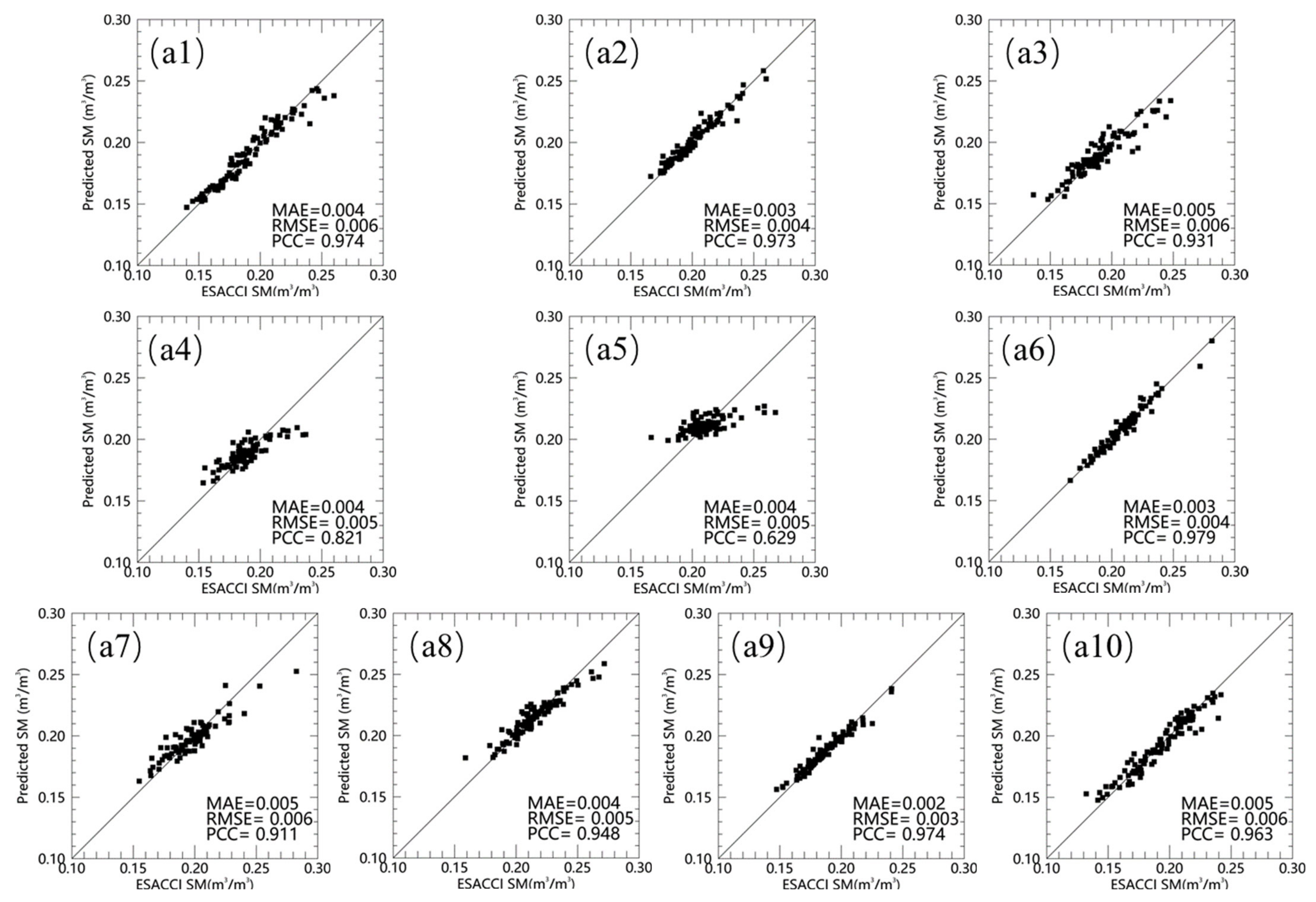
3.1. Overall Performance of the Retrieving and Downscaling SM

Due to the high latitude and relatively low temperatures in the selected study area, it is possible for the dielectric properties of water to vary between the months from October to April of the following year. Due to potential incomplete data on ESA-CCI products during this period, we have chosen to analyze data specifically from May to September. Furthermore, we have opted to examine a three-year dataset spanning from 2018 to 2020 in order to assess the accuracy of predicting SM at a resolution of 1 km.

Based on the algorithm employed, we have generated downscaled results for SM inversion under two different scenarios. Additionally, we conducted comparative analyses between the outcomes of a single model and an integrated model using the CatBoost algorithm to ascertain any variations between these approaches.

We selected MAE, RMSE, and PCC as evaluation metrics to analyze the results. Figure 5 illustrates the evaluation results using the CatBoost algorithm (Model 1), while

Table 2. The evaluation results based on the CatBoost algorithm.

	Model 1			Model 2
Time	MAE(m3/m3)	RMSE(m3/m3)	PCC	MAE(m3/m3)	RMSE(m3/m3)	PCC
9 May 2018	0.004	0.005	0.129	0.002	0.003	0.188
25 May 2018	0.005	0.007	0.042	0.003	0.004	0.490
10 June 2018	0.002	0.002	−0.116	0.001	0.002	0.007
26 June 2018	0.004	0.005	−0.013	0.004	0.005	0.503
12 July 2018	0.003	0.004	0.021	0.005	0.006	0.366
28 July 2018	0.004	0.005	0.009	0.005	0.006	−0.163
13 August 2018	0.004	0.004	0.074	0.003	0.004	0.341
29 August 2018	0.005	0.005	−0.131	0.009	0.012	0.310
14 September 2018	0.004	0.004	0.097	0.003	0.004	0.000
30 September 2018	0.005	0.006	0.095	0.007	0.009	−0.049
9 May 2019	0.006	0.007	−0.106	0.003	0.004	−0.376
25 May 2019	0.003	0.005	0.031	0.004	0.005	0.133
10 June 2019	0.004	0.005	−0.096	0.003	0.004	0.426
26 June 2019	0.002	0.003	−0.006	0.006	0.009	0.090
12 July 2019	0.004	0.005	−0.066	0.002	0.003	0.139
28 July 2019	0.008	0.021	0.274	0.003	0.003	0.459
13 August 2019	0.004	0.006	−0.054	0.003	0.004	−0.077
29 August 2019	0.006	0.022	0.106	0.003	0.004	0.185
14 September 2019	0.006	0.019	0.152	0.004	0.004	0.125
30 September 2019	0.006	0.017	0.180	0.006	0.008	0.128
9 May 2020	0.007	0.021	0.011	0.008	0.010	0.157
25 May 2020	0.006	0.022	0.089	0.003	0.004	0.396
10 June 2020	0.004	0.005	0.118	0.002	0.002	0.042
26 June 2020	0.002	0.002	0.024	0.005	0.007	−0.118
12 July 2020	0.004	0.004	0.016	0.002	0.002	0.388
28 July 2020	0.003	0.003	−0.070	0.003	0.004	0.039
13 August 2020	0.003	0.004	−0.068	0.004	0.005	−0.196
29 August 2020	0.004	0.005	−0.07	0.003	0.004	−0.268
14 September 2020	0.003	0.004	0.065	0.002	0.003	−0.025
30 September 2020	0.003	0.004	0.012	0.003	0.004	−0.001

provides a clear representation of these results.

In this section, MAE ranges from 0.002 to 0.008 m³/m³, and RMSE ranges from 0.017 to 0.022 m³/m³. However, the PCC ranges from −0.131 to 0.274. The evaluation results for retrieving and downscaling SM (SM) using the CatBoost algorithm during the period of 2019–2020 are displayed. It is worth noting that the reported outcomes correspond to Model 2, as depicted in Figure 6. The values for MAE and RMSE range from 0.001 to 0.009 m³/m³ and 0.002 to 0.01 m³/m³, respectively. Table 2 presents the minimum PCC value of −0.376 and the maximum value of 0.503. In Figure 7, we present the evaluation results derived from the Stacking algorithm (Model 1) during the period of 2018–2020. From both Figure 7 and

Table 3. The evaluation results based on the Stacking algorithm.

	Model 1			Model 2
Time	MAE(m3/m3)	RMSE(m3/m3)	PCC	MAE(m3/m3)	RMSE(m3/m3)	PCC
9 May 2018	0.008	0.010	0.814	0.004	0.005	0.953
25 May 2018	0.010	0.020	0.584	0.006	0.018	0.698
10 June 2018	0.008	0.017	0.180	0.006	0.018	0.698
26 June 2018	0.010	0.021	0.587	0.004	0.005	0.958
12 July 2018	0.010	0.024	0.429	0.005	0.006	0.835
28 July 2018	0.007	0.010	0.870	0.006	0.008	0.892
13 August 2018	0.011	0.026	0.388	0.006	0.007	0.891
29 August 2018	0.006	0.009	0.890	0.006	0.008	0.925
14 September 2018	0.012	0.025	0.332	0.003	0.004	0.973
30 September 2018	0.008	0.010	0.882	0.005	0.006	0.963
9 May 2018	0.011	0.021	0.768	0.004	0.006	0.974
25 May 2019	0.010	0.023	0.471	0.003	0.004	0.973
10 June 2019	0.007	0.009	0.866	0.005	0.006	0.931
26 June 2019	0.006	0.008	0.792	0.004	0.005	0.821
12 July 2019	0.006	0.007	0.761	0.004	0.005	0.629
28 July 2019	0.007	0.009	0.794	0.003	0.004	0.979
13 August 2019	0.011	0.024	0.509	0.005	0.006	0.911
29 August 2019	0.006	0.008	0.846	0.004	0.005	0.948
14 September 2019	0.005	0.008	0.837	0.002	0.003	0.974
30 September 2019	0.008	0.010	0.882	0.005	0.006	0.963
9 May 2020	0.011	0.021	0.768	0.004	0.004	0.979
25 May 2020	0.011	0.025	0.403	0.003	0.005	0.972
10 June 2020	0.005	0.007	0.833	0.003	0.004	0.962
26 June 2020	0.010	0.024	0.139	0.003	0.004	0.825
12 July 2020	0.009	0.012	0.744	0.006	0.007	0.848
28 July 2020	0.011	0.025	0.426	0.003	0.004	0.938
13 August 2020	0.010	0.024	0.35	0.002	0.003	0.979
29 August 2020	0.006	0.009	0.915	0.002	0.003	0.990
14 September 2020	0.01	0.012	0.678	0.003	0.004	0.977
30 September 2020	0.008	0.011	0.807	0.005	0.006	0.924

, we observe that the MAE ranges from 0.005 to 0.012 m³/m³, and the RMSE ranges from 0.007 to 0.26 m³/m³. Furthermore, the minimum PCC value is 0.18, and the maximum value is 0.915, according to Table 3. Lastly, Figure 8 shows the results obtained from the Stacking algorithm (Model 2) in 2018–2020. The range of MAE, RMSE, and PCC is reported as 0.002–0.03 m³/m³, 0.003–0.018 m³/m³, and 0.629–0.990 respectively.

By employing the CatBoost algorithm as a single model and combining it with the integrated learning stacking algorithm, we observed that the overall MAE and RMSE accuracy of the CatBoost algorithm was marginally superior to the stacking algorithm. However, evaluations based on PCC revealed consistently low values for both instances of the CatBoost algorithm, suggesting a weak correlation between the predicted SM results and the ESA-CCI SM data. Conversely, the Stacking model utilizing the integrated learning algorithm exhibited significantly improved PCC compared to the CatBoost algorithm. Notably, in Model 2, there existed a strong correlation between the predicted SM results and ESA-CCI data.

Figure 9, Figure 10 and Figure 11 illustrate the spatial distribution of SM at a resolution of 1 km, which was obtained through the downscaling of model. Meanwhile, Figure A1, Figure A2 and Figure A3 display the corresponding 1 km SM distribution maps generated by Model 2. Furthermore, Figure A4, Figure A5 and Figure A6 present the 25 km SM distribution maps based on the ESA-CCI product (shown in Appendix A). The selection of the time period for our study analysis was focused on the months from May to September, covering the years 2018 to 2020. This decision was motivated by the fact that May to September represents the primary period of vegetation growth in the study area. Given that our objective is to investigate the variations in SM within the vegetation cover area, we ultimately opted for these specified months. The numbers 1–10 represent the dates of mid to late May, mid to late June, mid to late July, mid to late August, and mid to late September. These ten occurrences mark specific time periods throughout the year.

We observe that the SM range in this study area is predominantly distributed between 0 and 0.4 m³/m³. The blue section represents low SM values, while the red section indicates high SM values. Visually, we can deduce that both methods exhibit similar SM distribution patterns as observed in EAS-CCI data. This correspondence supports the efficacy of our proposed methodologies in accurately capturing the spatial distribution of SM at a resolution of 1 km.

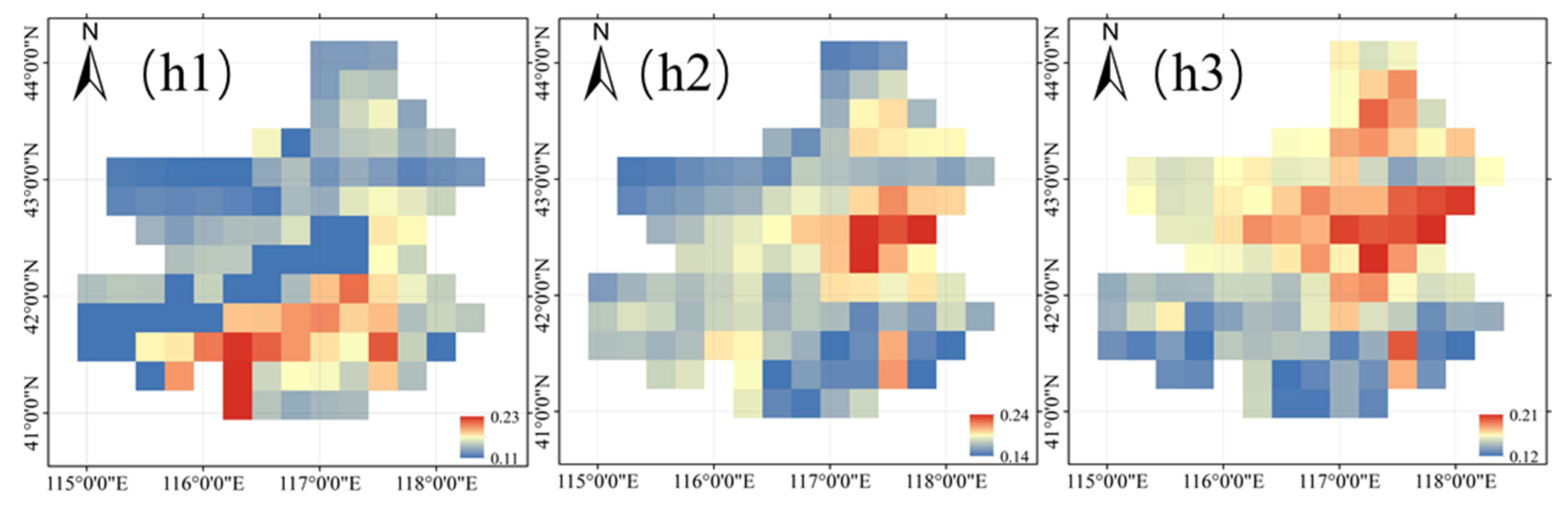
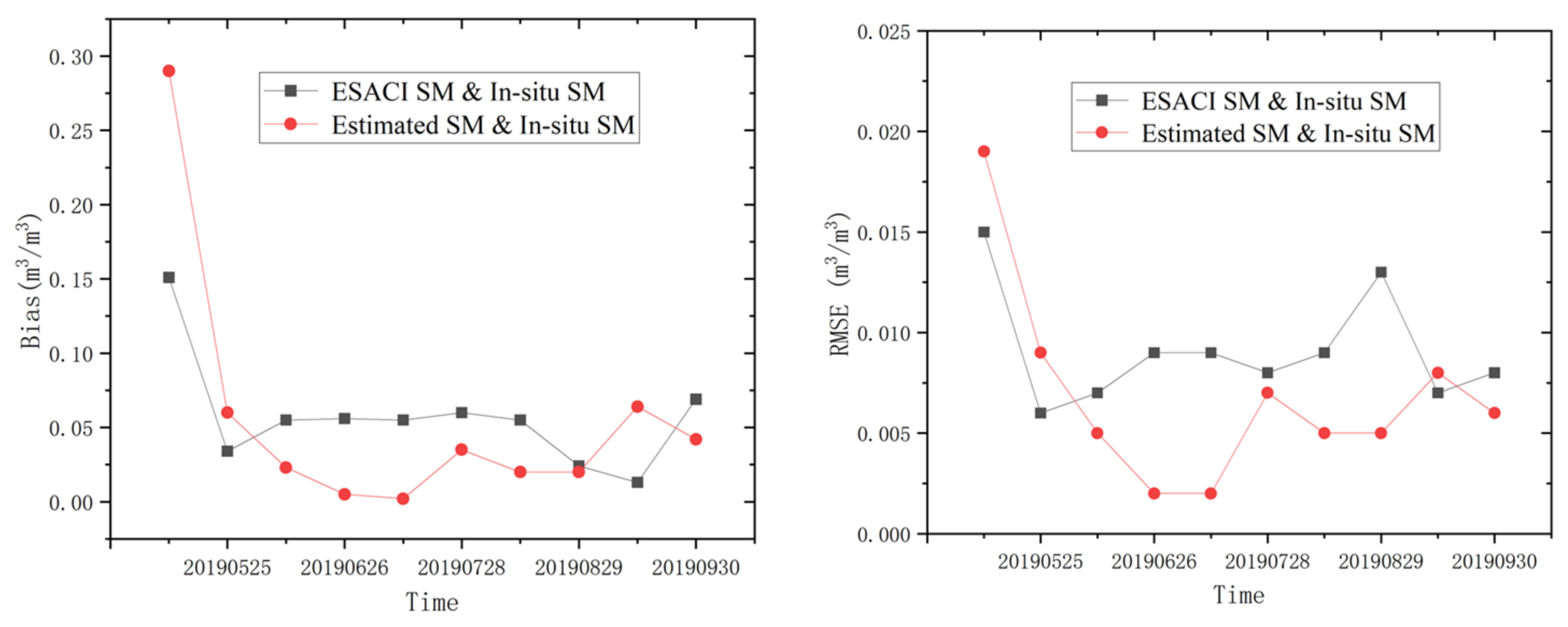
3.2. Evaluation with In Situ Measurements

Through the analysis in Section 3.1, it was discovered that the stacking algorithm, which combines multiple models, exhibits higher precision compared to the CatBoost algorithm that relies on a single model. Additionally, the accuracy of the stacking algorithm with Model 2 outperforms that of Model 1. Figure 12 is a histogram comparing the results of Model 1 and Model 2. This study employs a two-model approach for SM estimation and downscaling, each demonstrating enhanced accuracy in deriving SM results. Model 2 exhibits a slightly superior performance compared to Model 1. Our analysis indicates that within Model 2, there is a discernible trend showcasing a more pronounced interrelation among various variables. This strengthened interdependency potentially leads to a reduction in the presence of outliers within the dataset. As a result, the establishment of a tighter relationship among these variables significantly bolsters the fitting effect during the estimation and downscaling processes. The enhanced interrelationship among variables in Model 2 plays a pivotal role in refining the accuracy of SM estimation. By virtue of this reinforced relationship, the model demonstrates an improved capacity to capture the complex interactions and dependencies among the variables contributing to SM dynamics. Consequently, this refined understanding and alignment among the variables lead to a more precise representation of SM distribution, elevating the overall accuracy of the estimation and downscaling techniques applied within Model 2.

In this segment, we meticulously selected specific observed data from the following dates in 2019: May 9, May 25, June 10, June 26, July 12, July 28, August 13, August 29, September 14, and September 30. We conducted comparative analyses between the measured data for these individual dates and the corresponding estimated SM data generated by employing our algorithm.

For each of these dates, we systematically compared the measured data obtained on the specified date with the SM estimations derived from our algorithm. We calculated two key metrics, Bias (Bais) and Root Mean Square Error (RMSE), to perform a comprehensive analysis. Each day’s dataset consisted of 31–35 sample points.

Subsequently, the Bias and RMSE values computed for the ten different dates were visualized in line charts. This visual representation allowed for a comparative assessment, offering insights into the differences and trends between the measured data and the SM estimations obtained through our algorithm for each respective date. The outcomes of the Bias and RMSE analysis for 2019 using Stacking algorithm Model 2 are presented in Figure 13 and

Table 4. The results of Bias and RMSE in 2019 with the Stacking algorithm Model 2: ESACI SM and in situ SM, estimated SM and in situ SM.

	ESACI SM & In Situ SM		Estimated SM & In Situ SM
Time	Bais (m3/m3)	RMSE (m3/m3)	Bais (m3/m3)	RMSE (m3/m3)
9 May 2019	0.151	0.015	0.290	0.019
25 May 2019	0.034	0.006	0.060	0.009
10 June 2019	0.055	0.007	0.023	0.005
26 June 2019	0.056	0.009	0.005	0.002
12 July 2019	0.055	0.009	0.002	0.002
28 July 2019	0.06	0.008	0.035	0.007
13 August 2019	0.055	0.009	0.020	0.005
29 August 2019	0.024	0.013	0.020	0.005
14 September 2019	0.013	0.007	0.064	0.008
30 September 2019	0.069	0.008	0.042	0.006

, respectively.

Figure 13 displays a line chart depicting BIAS and RMSE, illustrating the observed trend from May to September. During this period, both BIAS and RMSE values calculated from predicted and measured SM were slightly higher compared to those calculated from ESACI SM and measured SM. Specifically, for the months of May and mid-September, the BIAS and RMSE results for ESACI SM and in situ SM were 0.151 m³/m³, 0.034 m³/m³, 0.013 m³/m³, and 0.015 m³/m³, 0.006 m³/m³, 0.007 m³/m³, respectively. Conversely, when considering predicted results and in situ SM, the BIAS and RMSE values were 0.29 m³/m³, 0.06 m³/m³, 0.064 m³/m³, and 0.19 m³/m³, 0.009 m³/m³, 0.008 m³/m³, as shown in Table 4. From mid-June to late August and late September, the accuracy of estimated SM and in situ SM meters decreased, as evident in Figure 13 and Table 4. However, the 1 km SM data predicted based on stacking yielded more precise results.

We conducted an accuracy analysis using in situ SM data, as well as separately comparing the predicted results and ESACI SM data. Although there were minor differences among the results, both the predicted results and ESACI SM data showed good accuracy in relation to the actual SM. Consequently, we further analyzed the accuracy of the ESACI SM data using the predicted results, as illustrated in Figure A3.

Figure 14 illustrates a histogram analysis depicting the relationship between Estimated SM and ESA-CCI SM for the year 2019. The figure illustrates a scatterplot representing the relationship between predicted SM and ESA-CCI SM in 2019 (Figure 15). The results reveal a robust correlation between the predicted and ESA-CCI SM, with a maximum PCC value of 0.979 and a minimum of 0.629. These PCC values indicate a strong linear relationship between predicted and ESA-CCI SM. PCC is a statistical measure of the strength of a linear relationship between two variables, where values approaching 1 signify a stronger positive correlation.

Notably, instances with higher PCC values typically correspond to smaller MAE and RMSE values. MAE ranges between 0.002 to 0.005 m³/m³, while RMSE ranges from 0.003 to 0.006 m³/m³. This suggests minimal deviation between predicted and observed values, showcasing a high consistency between predicted SM and ESA-CCI data. Overall, higher PCC values indicate a stronger linear relationship between predicted and ESA-CCI SM, while smaller MAE and RMSE values reflect higher predictive accuracy. Furthermore, Model 2 demonstrates greater accuracy compared to Model 1, with Model 1 exhibiting some instability. This suggests that Model 2 better captures the variability in SM.

Considering the dual evaluation against ESA-CCI products and measured data, our proposed method proves feasible for studying SM in this specific area. The high similarity in PCC values underscores the method’s reliability in estimating SM. Furthermore, the consistency portrayed by the PCC values, indicative of a robust correlation between the estimated SM and ESA-CCI SM, substantiates the method’s capacity to reliably capture variations in SM dynamics. This suggests that our approach not only establishes feasibility but also highlights its potential for nuanced insights into the intricate SM patterns within this specific geographical domain.

4. Discussion

Based on the stacking-based integrated learning algorithm for SM downscaling depicted in Figure 3 and Figure 4, our objective is to investigate the potential of a multi-model stacking-based algorithm in generating high-resolution SM products with improved accuracy. Table 2 and Table 3 present the results obtained from two different modes: one utilizing the CatBoost algorithm and the other employing the stacking algorithm. It is evident that the stacking algorithm, which incorporates multiple models, outperforms the CatBoost algorithm. Despite the fact that the CatBoost algorithm also achieves lower MAE and RMSE, the PCC values calculated for SM prediction and ESA-CCI SM exhibit a significant decrease. This suggests that the prediction results are less correlated with ESA-CCI SM. In contrast, our developed stacking algorithm yields superior outcomes in both models, particularly in Model 2. Here, we not only achieve lower MAE and RMSE but also higher PCC. This outcome corroborates that the improved performance of the stacking algorithm can be attributed to the integration of multiple models rather than relying solely on one individual model.

While the majority of research on SM inversion and downscaling algorithms has centered around single models, there has been limited attention given to the development of multi-model integration algorithms [81,82,83,84]. The multi-model integration algorithm stacking was chosen for its ability to combine the prediction results of multiple models, resulting in improved and robust predictions compared to individual models. One of the major advantages of stacking is its efficiency and utilization of all parameters in the training dataset. The approach involves building multiple first-level learners of different types to obtain initial predictions and then constructing a second-level learner based on these first-level predictions to generate final predictions. The motivation behind using stacking can be described as follows: if a first-level learner incorrectly learns a region of the feature space, the second-level learner can correct this error by incorporating the learning behaviors of other first-level learners. It should be noted that the input data selected for this study, namely LST, NDVI, ET, and SR, are commonly used in SM inversion research. Numerous studies have demonstrated a strong correlation between these parameters and SM [85,86,87,88,89]. LST can reflect the energy exchange between the surface and the atmosphere, and the amount of soil moisture directly affects this energy exchange process, making LST closely related to SM. NDVI is an important indicator for measuring vegetation growth, as vegetation absorbs water from the soil through its roots, and its growth status is closely related to soil moisture content. Therefore, there is an intrinsic connection between NDVI and SM. ET, as a key process of water transfer from the surface to the atmosphere, is directly constrained by soil moisture, and the correlation between the two is evident. SR can sensitively capture changes in the physical and chemical properties of the soil surface, which are closely linked to variations in soil moisture content.

In addition, recent studies have highlighted the significant influence of Digital Elevation Model (DEM) variation on SM. It has been found that changes in SM often coincide with alterations in the topography [56]. Factors such as terrain undulations, slope steepness, and variations in aspect can significantly impact the distribution of precipitation, the direction of surface runoff, as well as the infiltration and evaporation processes of soil moisture, thereby causing changes in the spatial distribution of SM. Although numerous studies have utilized these covariates, the majority of them have focused on a limited number of covariates for SM retrieval and downscaling. The primary objective of this paper is to select a more comprehensive set of characteristic parameters and examine whether combining these parameters can lead to highly accurate and applicable results. In this study, the analysis of SM downscaling was conducted separately using two distinct models within the established stacking framework, resulting in relatively satisfactory accuracy. These findings hold significance for the prediction and direction of SM downscaling.

Meanwhile, the findings presented in Table 3 reveal that Model 2 consistently yields higher PCC values compared to Model 1. This distinction may be attributed to the sampling process employed in Model 2. Specifically, each parameter is initially resampled to 25 km using ESA-CCI SM inversion, resulting in a more refined representation of SM at this resolution. Consequently, each parameter can establish a complex nonlinear relationship with ESA-CCI, leading to more accurate results. On the other hand, while Model 1 boasts higher accuracy for each input variable and more precise values for each image element, the discrepancy arises from the resampling of ESA-CCI SM to 1 km prior to analysis. This resampling process introduces inaccuracies in the final 1 km SM estimations, deviating from the original ESA-CCI SM data. Hence, the calculated PCC shows a significant decrease.

In this study, we selected two models for SM downscaling research. Model 1, during the process of downscaling data from high resolution to low resolution, may lose some detailed information, leading to a certain deviation between the downscaled data and the actual observed values. As a result, the fitting degree of the estimation model on the downscaled data may be limited, especially for models or data that are sensitive to local details. On the other hand, Model 2 can make better use of the information from the original data during the estimation process, resulting in estimation results that are closer to the actual observed values. When downscaling the estimated results to the target resolution, appropriate interpolation or averaging methods can be used to maintain the spatial consistency and continuity of the data. Therefore, this method generally performs better in terms of fitting, especially when local detail information needs to be preserved.

However, our study has several limitations that need to be addressed. Firstly, our focus is on the 16-day high-resolution SM prediction and downscaling. While this provides valuable insights, it is important to consider the significance of daily high-resolution SM data, especially during the vegetation growth period, for agricultural production. Furthermore, the time-resolved products generated in our study have greater relevance for the entire growth cycle of vegetation crops. However, the accuracy of these continuous time products may be affected by the limited availability of effective data from SM monitoring sites within the selected study area. The absence of ground observation data and the presence of discontinuous rows introduce additional uncertainties to our findings. In order to expand the scope of our method and assess its feasibility and adaptability in different regions, it would be beneficial to incorporate ground data from various locations. This approach would enable us to obtain high-precision SM products across different regions and a broader geographic scale.

5. Conclusions

We developed a multi-model fusion stacking algorithm for conducting an SM downscaling study. The input parameters for the model included LST, NDVI, ET, SR, and topography-related features. We utilized daily data from the ESA-CCI SM 25 km dataset to obtain 16 days of high-resolution (1 km) SM data. Our findings indicate that the integrated model-based stacking algorithm demonstrates superior accuracy and stability compared to a single model approach using the CatBoost algorithm. To minimize data variability, we collected three years of data (2018–2020) from May to September. Additionally, we proposed two approaches for the downscaling process: one involved downscaling first and then inversion, while the other involved inversion first and then downscaling. We successively applied the stacking algorithm to both cases using high-precision 1 km SM products. The results show that both methods yield accurate results, but the inversion followed by the downscaling approach is relatively better, exhibiting higher PCC (Pearson correlation coefficient). We compared the predicted SM and ESA-CCI SM; it is evident that the predicted results exhibit a strong correlation with ESA-CCI SM, with a maximum PCC value of 0.979 and a minimum value of 0.629. The MAE values range from 0.002 to 0.005 m³/m³, and the RMSE ranges from 0.003 to 0.006 m³/m³. Despite achieving favorable outcomes, our established algorithm does have certain limitations. In the current study, although some good results have been achieved using the stacking algorithm, there are still many issues and areas for improvement. For example, the current study area is small, and longer time series data have not been utilized.

In future research, it will be necessary to expand the study area, incorporate longer time series data, and explore methods that provide higher temporal resolution in order to obtain large-scale SM products with high spatial and temporal resolution.

References

1. Babaeian, E.; Sadeghi, M.; Jones, S.B.; Montzka, C.; Vereecken, H.; Tuller, M. Ground, Proximal, and Satellite Remote Sensing of Soil Moisture. Rev. Geophys. 2019, 57, 530–616. [Google Scholar] [CrossRef]
2. Li, Z.L.; Leng, P.; Zhou, C.H.; Chen, K.S.; Zhou, F.C.; Shang, G.F. Soil moisture retrieval from remote sensing measurements: Current knowledge and directions for the future. Earth-Sci. Rev. 2021, 218, 103673. [Google Scholar] [CrossRef]
3. Huang, S.Z.; Zhang, X.; Chen, N.C.; Li, B.Y.; Ma, H.L.; Xu, L.; Li, R.H.; Niyogi, D. Drought propagation modification after the construction of the Three Gorges Dam in the Yangtze River Basin. J. Hydrol. 2021, 603, 127138. [Google Scholar] [CrossRef]
4. Srivastava, P.K. Satellite Soil Moisture: Review of Theory and Applications in Water Resources. Water Resour. Manag. 2017, 31, 3161–3176. [Google Scholar] [CrossRef]
5. Xue, Z.H.; Zhang, Y.J.; Zhang, L.; Li, H. Ensemble Learning Embedded with Gaussian Process Regression for Soil Moisture Estimation: A Case Study of the Continental US. IEEE Trans. Geosci. Remote Sens. 2022, 60, 4508817. [Google Scholar] [CrossRef]
6. Gao, Y.; Gao, M.F.; Wang, L.G.; Rozenstein, O. Soil Moisture Retrieval over a Vegetation-Covered Area Using ALOS-2 L-Band Synthetic Aperture Radar Data. Remote Sens. 2021, 13, 3894. [Google Scholar] [CrossRef]
7. Cui, H.; Jiang, L.; Paloscia, S.; Santi, E.; Pettinato, S.; Wang, J.; Fang, X.; Liao, W. The Potential of ALOS-2 and Sentinel-1 Radar Data for Soil Moisture Retrieval with High Spatial Resolution over Agroforestry Areas, China. IEEE Trans. Geosci. Remote 2021, 60, 1–17. [Google Scholar] [CrossRef]
8. Liu, Y.; Qian, J.X.; Yue, H. Combined Sentinel-1A with Sentinel-2A to Estimate Soil Moisture in Farmland. IEEE J. Sel. Top. Appl. Earth Obs. Remote Sens. 2021, 14, 1292–1310. [Google Scholar] [CrossRef]
9. Wang, J.J.; Wu, F.; Shang, J.L.; Zhou, Q.; Ahmad, I.; Zhou, G.S. Saline soil moisture mapping using Sentinel-1A synthetic aperture radar data and machine learning algorithms in humid region of China’s east coast. Catena 2022, 213, 106189. [Google Scholar] [CrossRef]
10. Entekhabi, D.; Njoku, E.; O’Neill, P.; Kellogg, K.; Entin, J. The NASA Soil Moisture Active Passive (SMAP) mission formulation. In Proceedings of the 2011 IEEE International Geoscience and Remote Sensing Symposium, Vancouver, BC, Canada, 24–29 July 2011; pp. 2302–2305. [Google Scholar] [CrossRef]
11. Kerr, Y.H.; Waldteufel, P.; Richaume, P.; Wigneron, J.P.; Ferrazzoli, P.; Mahmoodi, A.; Al Bitar, A.; Cabot, F.; Gruhier, C.; Juglea, S.E.; et al. The SMOS Soil Moisture Retrieval Algorithm. IEEE Trans. Geosci. Remote Sens. 2012, 50, 1384–1403. [Google Scholar] [CrossRef]
12. Wagner, W.; Hahn, S.; Kidd, R.; Melzer, T.; Bartalis, Z.; Hasenauer, S.; Figa-Saldaña, J.; De Rosnay, P.; Jann, A.; Schneider, S.; et al. The ASCAT Soil Moisture Product: A Review of its Specifications, Validation Results, and Emerging Applications. Meteorol. Z. 2013, 22, 5–33. [Google Scholar] [CrossRef]
13. Imaoka, K.; Kachi, M.; Fujii, H.; Murakami, H.; Hori, M.; Ono, A.; Igarashi, T.; Nakagawa, K.; Oki, T.; Honda, Y.; et al. Global Change Observation Mission (GCOM) for Monitoring Carbon, Water Cycles, and Climate Change. Proc. IEEE 2010, 98, 717–734. [Google Scholar] [CrossRef]
14. Shi, J.; Jiang, L.; Zhang, L.; Chen, K.; Wigneron, J.; Chanzy, A.; Jackson, T. Physically Based Estimation of Bare-Surface Soil Moisture With the Passive Radiometers. IEEE Trans. Geosci. Remote Sens. 2006, 44, 3145–3153. [Google Scholar] [CrossRef]
15. Gruber, A.; Dorigo, W.A.; Crow, W.; Wagner, W. Triple Collocation-Based Merging of Satellite Soil Moisture Retrievals. IEEE Trans. Geosci. Remote Sens. 2017, 55, 6780–6792. [Google Scholar] [CrossRef]
16. Dorigo, W.; Wagner, W.; Albergel, C.; Albrecht, F.; Balsamo, G.; Brocca, L.; Chung, D.; Ertl, M.; Forkel, M.; Gruber, A.; et al. ESA CCI Soil Moisture for improved Earth system understanding: State-of-the art and future directions. Remote Sens. Environ. 2017, 203, 185–215. [Google Scholar] [CrossRef]
17. Gruber, A.; Scanlon, T.; van der Schalie, R.; Wagner, W.; Dorigo, W. Evolution of the ESA CCI Soil Moisture climate data records and their underlying merging methodology. Earth Syst. Sci. Data 2019, 11, 717–739. [Google Scholar] [CrossRef]
18. Lauer, A.; Eyring, V.; Righi, M.; Buchwitz, M.; Defourny, P.; Evaldsson, M.; Friedlingstein, P.; de Jeu, R.; de Leeuw, G.; Loew, A.; et al. Benchmarking CMIP5 models with a subset of ESA CCI Phase 2 data using the ESMValTool. Remote Sens. Environ. 2017, 203, 9–39. [Google Scholar] [CrossRef]
19. Plummer, S.; Lecomte, P.; Doherty, M. The ESA Climate Change Initiative (CCI): A European contribution to the generation of the Global Climate Observing System. Remote Sens. Environ. 2017, 203, 2–8. [Google Scholar] [CrossRef]
20. Zhang, L.Q.; Liu, Y.; Ren, L.L.; Jiang, S.H.; Yang, X.L.; Yuan, F.; Wang, M.H.; Wei, L.Y. Drought Monitoring and Evaluation by ESA CCI Soil Moisture Products Over the Yellow River Basin. IEEE J. Sel. Top. Appl. Earth Obs. Remote Sens. 2019, 12, 3376–3386. [Google Scholar] [CrossRef]
21. Zhao, W.; Wen, F.; Wang, Q.; Sanchez, N.; Piles, M. Seamless downscaling of the ESA CCI soil moisture data at the daily scale with MODIS land products. J. Hydrol. 2021, 603, 126930. [Google Scholar] [CrossRef]
22. Huang, S.Z.; Zhang, X.; Wang, C.; Chen, N.C. Two-step fusion method for generating 1 km seamless multi-layer soil moisture with high accuracy in the Qinghai-Tibet plateau. Isprs J. Photogramm. Remote Sens. 2023, 197, 346–363. [Google Scholar] [CrossRef]
23. Sishah, S.; Abrahem, T.; Azene, G.; Dessalew, A.; Hundera, H. Downscaling and validating SMAP soil moisture using a machine learning algorithm over the Awash River basin, Ethiopia. PLoS ONE 2023, 18, e0279895. [Google Scholar] [CrossRef]
24. Sun, H.; Gao, J.H. A pixel-wise calculation of soil evaporative efficiency with thermal/optical remote sensing and meteorological reanalysis data for downscaling microwave soil moisture. Agric. Water Manag. 2023, 276, 108063. [Google Scholar] [CrossRef]
25. Wakigari, S.A.; Leconte, R. Exploring the utility of the downscaled SMAP soil moisture products in improving streamflow simulation. J. Hydrol. Reg. Stud. 2023, 47, 101380. [Google Scholar] [CrossRef]
26. Wang, Y.; Li, R.A.; Liang, M.; Ma, J.F.; Yang, Y.Z.; Zheng, H. Impact of crop types and irrigation on soil moisture downscaling in water-stressed cropland regions. Environ. Impact Assess. Rev. 2023, 100, 7073. [Google Scholar] [CrossRef]
27. Leng, P.; Yang, Z.; Yan, Q.Y.; Shang, G.F.; Zhang, X.; Han, X.J.; Li, Z.L. A framework for estimating all-weather fine resolution soil moisture from the integration of physics-based and machine learning-based algorithms. Comput. Electron. Agric. 2023, 206, 107673. [Google Scholar] [CrossRef]
28. Judge, J.; Liu, P.W.; Monsiváis-Huertero, A.; Bongiovanni, T.; Chakrabarti, S.; Steele-Dunne, S.C.; Preston, D.; Allen, S.; Bermejo, J.P.; Rush, P.; et al. Impact of vegetation water content information on soil moisture retrievals in agricultural regions: An analysis based on the SMAPVEX16-MicroWEX dataset. Remote Sens. Environ. 2021, 265, 112623. [Google Scholar] [CrossRef]
29. Tao, S.Y.; Zhang, X.; Feng, R.; Qi, W.C.; Wang, Y.B.; Shrestha, B. Retrieving soil moisture from grape growing areas using multi-feature and stacking-based ensemble learning modeling. Comput. Electron. Agric. 2023, 204, 107537. [Google Scholar] [CrossRef]
30. He, L.; Cheng, Y.; Li, Y.X.; Li, F.; Fan, K.L.; Li, Y.Z. An Improved Method for Soil Moisture Monitoring With Ensemble Learning Methods Over the Tibetan Plateau. IEEE J. Sel. Top. Appl. Earth Obs. Remote Sens. 2021, 14, 2833–2844. [Google Scholar] [CrossRef]
31. Zhang, F.; Zhang, L.-W.; Shi, J.-J.; Huang, J.-F. Soil Moisture Monitoring Based on Land Surface Temperature-Vegetation Index Space Derived from MODIS Data. Pedosphere 2014, 24, 450–460. [Google Scholar] [CrossRef]
32. Bai, L.; Long, D.; Yan, L. Estimation of Surface Soil Moisture With Downscaled Land Surface Temperatures Using a Data Fusion Approach for Heterogeneous Agricultural Land. Water Resour. Res. 2019, 55, 1105–1128. [Google Scholar] [CrossRef]
33. Rawat, K.S.; Sehgal, V.K.; Singh, S.K.; Ray, S.S. Soil moisture estimation using triangular method at higher resolution from MODIS products—ScienceDirect. Phys. Chem. Earth Parts A/B/C 2022, 126, 103051. [Google Scholar] [CrossRef]
34. Younis, S.M.; Iqbal, J. Estimation of soil moisture using multispectral and FTIR techniques. Egypt. J. Remote Sens. Space Sci. 2015, 18, 151–161. [Google Scholar] [CrossRef]
35. Piles, M.; Camps, A.; Vall-llossera, M.; Corbella, I.; Panciera, R.; Rudiger, C.; Kerr, Y.H.; Walker, J. Downscaling SMOS-Derived Soil Moisture Using MODIS Visible/Infrared Data. IEEE Trans. Geosci. Remote Sens. 2011, 49, 3156–3166. [Google Scholar] [CrossRef]
36. Zhang, W.; Koch, J.; Wei, F.L.; Zeng, Z.Z.; Fang, Z.X.; Fensholt, R. Soil Moisture and Atmospheric Aridity Impact Spatio-Temporal Changes in Evapotranspiration at a Global Scale. J. Geophys. Res. Atmos. 2023, 128, e2022JD038046. [Google Scholar] [CrossRef]
37. Weidong, L.; Baret, F.; Xingfa, G.; Qingxi, T.; Lanfen, Z.; Bing, Z. Relating soil surface moisture to reflectance. Remote Sens. Environ. 2002, 81, 238–246. [Google Scholar] [CrossRef]
38. Singh, A.; Gaurav, K. Deep learning and data fusion to estimate surface soil moisture from multi-sensor satellite images. Sci. Rep. 2023, 13, 2251. [Google Scholar] [CrossRef]
39. Adab, H.; Morbidelli, R.; Saltalippi, C.; Moradian, M.; Ghalhari, G.A.F. Machine Learning to Estimate Surface Soil Moisture from Remote Sensing Data. Water 2020, 12, 3223. [Google Scholar] [CrossRef]
40. Nolet, C.; Poortinga, A.; Roosjen, P.; Bartholomeus, H.; Ruessink, G. Measuring and Modeling the Effect of Surface Moisture on the Spectral Reflectance of Coastal Beach Sand. PLoS ONE 2014, 9, e112151. [Google Scholar] [CrossRef]
41. Bowers, S.A.; Smith, S.J. Spectrophotometric Determination of Soil Water Content. Soil Sci. Soc. Am. J. 1972, 36, 978–980. [Google Scholar] [CrossRef]
42. Robinove, C.J.; Chavez, P.S.; Gehring, D.; Holmgren, R. Arid land monitoring using Landsat albedo difference images. Remote Sens. Environ. 1981, 11, 133–156. [Google Scholar] [CrossRef]
43. Knadel, M.; Castaldi, F.; Barbetti, R.; Ben-Dor, E.; Gholizadeh, A.; Lorenzetti, R. Mathematical techniques to remove moisture effects from visible-near-infrared-shortwave-infrared soil spectra-review. Appl. Spectrosc. Rev. 2023, 58, 629–662. [Google Scholar] [CrossRef]
44. Soriano-Disla, J.M.; Janik, L.J.; Rossel, R.A.V.; Macdonald, L.M.; McLaughlin, M.J. The Performance of Visible, Near-, and Mid-Infrared Reflectance Spectroscopy for Prediction of Soil Physical, Chemical, and Biological Properties. Appl. Spectrosc. Rev. 2014, 49, 139–186. [Google Scholar] [CrossRef]
45. Watson, K. Regional Thermal-Inertia Mapping from an Experimental Satellite. Geophysics 1982, 47, 1681–1687. [Google Scholar] [CrossRef]
46. Jackson, R.D. Soil Moisture Inferences from Thermal-Infrared Measurements of Vegetation Temperatures. IEEE Trans. Geosci. Remote Sens. 1982, GE-20, 282–286. [Google Scholar] [CrossRef]
47. Leng, P.; Song, X.; Li, Z.-L.; Ma, J.; Zhou, F.; Li, S. Bare surface soil moisture retrieval from the synergistic use of optical and thermal infrared data. Int. J. Remote Sens. 2014, 35, 988–1003. [Google Scholar] [CrossRef]
48. Sánchez-Ruiz, S.; Piles, M.; Sánchez, N.; Martínez-Fernández, J.; Vall-llossera, M.; Camps, A. Combining SMOS with visible and near/shortwave/thermal infrared satellite data for high resolution soil moisture estimates. J. Hydrol. 2014, 516, 273–283. [Google Scholar] [CrossRef]
49. Yang, Y.; Guan, H.; Long, D.; Liu, B.; Qin, G.; Qin, J.; Batelaan, O. Estimation of Surface Soil Moisture from Thermal Infrared Remote Sensing Using an Improved Trapezoid Method. Remote Sens. 2015, 7, 8250–8270. [Google Scholar] [CrossRef]
50. Wu, X.J.; Wen, J. Recent Progress on Modeling Land Emission and Retrieving Soil Moisture on the Tibetan Plateau Based on L-Band Passive Microwave Remote Sensing. Remote Sens. 2022, 14, 4191. [Google Scholar] [CrossRef]
51. Zheng, D.H.; Wang, X.; van der Velde, R.; Ferrazzoli, P.; Wen, J.; Wang, Z.L.; Schwank, M.; Colliander, A.; Bindlish, R.; Su, Z.B. Impact of surface roughness, vegetation opacity and soil permittivity on L-band microwave emission and soil moisture retrieval in the third pole environment. Remote Sens. Environ. 2018, 209, 633–647. [Google Scholar] [CrossRef]
52. Mavrovic, A.; Sonnentag, O.; Lemmetyinen, J.; Baltzer, J.L.; Kinnard, C.; Roy, A. Reviews and syntheses: Recent advances in microwave remote sensing insupport of terrestrial carbon cycle science in Arctic-boreal regions. Biogeosciences 2023, 20, 2941–2970. [Google Scholar] [CrossRef]
53. Abdollahipour, A.; Ahmadi, H.; Aminnejad, B. A review of downscaling methods of satellite-based precipitation estimates. Earth Sci. Inform. 2022, 15, 1–20. [Google Scholar] [CrossRef]
54. Peng, J.; Loew, A.; Merlin, O.; Verhoest, N.E.C. A review of spatial downscaling of satellite remotely sensed soil moisture. Rev. Geophys. 2017, 55, 341–366. [Google Scholar] [CrossRef]
55. Im, J.; Park, S.; Rhee, J.; Baik, J.; Choi, M. Downscaling of AMSR-E soil moisture with MODIS products using machine learning approaches. Environ. Earth Sci. 2016, 75, 1120. [Google Scholar] [CrossRef]
56. Liu, Y.; Jing, W.; Wang, Q.; Xia, X. Generating high-resolution daily soil moisture by using spatial downscaling techniques: A comparison of six machine learning algorithms. Adv. Water Resour. 2020, 141, 103601. [Google Scholar] [CrossRef]
57. Zhao, H.F.; Li, J.; Yuan, Q.Q.; Lin, L.P.; Yue, L.W.; Xu, H.Z. Downscaling of soil moisture products using deep learning: Comparison and analysis on Tibetan Plateau. J. Hydrol. 2022, 607, 127570. [Google Scholar] [CrossRef]
58. Alemohammad, S.H.; Kolassa, J.; Prigent, C.; Aires, F.; Gentine, P. Global downscaling of remotely sensed soil moisture using neural networks. Hydrol. Earth Syst. Sci. 2018, 22, 5341–5356. [Google Scholar] [CrossRef]
59. Guevara, M.; Vargas, R. Downscaling satellite soil moisture using geomorphometry and machine learning. PLoS ONE 2019, 14, e0219639. [Google Scholar] [CrossRef]
60. Cui, Y.K.; Chen, X.; Xiong, W.T.; He, L.; Lv, F.; Fan, W.J.; Luo, Z.L.; Hong, Y. A Soil Moisture Spatial and Temporal Resolution Improving Algorithm Based on Multi-Source Remote Sensing Data and GRNN Model. Remote Sens. 2020, 12, 455. [Google Scholar] [CrossRef]
61. Sun, H.; Cui, Y.J. Evaluating Downscaling Factors of Microwave Satellite Soil Moisture Based on Machine Learning Method. Remote Sens. 2021, 13, 133. [Google Scholar] [CrossRef]
62. Shangguan, Y.L.; Min, X.X.; Shi, Z. Inter-comparison and integration of different soil moisture downscaling methods over the Qinghai-Tibet Plateau. J. Hydrol. 2023, 617, 129014. [Google Scholar] [CrossRef]
63. Hegazi, E.H.; Yang, L.B.; Huang, J.F. A Convolutional Neural Network Algorithm for Soil Moisture Prediction from Sentinel-1 SAR Images. Remote Sens. 2021, 13, 4964. [Google Scholar] [CrossRef]
64. Rabiei, S.; Jalilvand, E.; Tajrishy, M. A Method to Estimate Surface Soil Moisture and Map the Irrigated Cropland Area Using Sentinel-1 and Sentinel-2 Data. Sustainability 2021, 13, 11355. [Google Scholar] [CrossRef]
65. El Hajj, M.; Baghdadi, N.; Zribi, M. Comparative analysis of the accuracy of surface soil moisture estimation from the C- and L-bands. Int. J. Appl. Earth Obs. Geoinf. 2019, 82, 101888. [Google Scholar] [CrossRef]
66. Yin, Q.; Li, J.L.; Zhou, Y.S.; Xiang, D.L.; Zhang, F. Adaptive weighted learning for vegetation contribution in soil moisture inversion using PolSAR data. Int. J. Remote Sens. 2022, 43, 3190–3215. [Google Scholar] [CrossRef]
67. Im, J.; Park, S.; Park, S.; Rhee, J. AMSR2 soil moisture downscaling using multisensor products through machine learning approach. In Proceedings of the IEEE International Geoscience & Remote Sensing Symposium, Milan, Italy, 26–31 July 2015. [Google Scholar] [CrossRef]
68. Kshatri, S.S.; Singh, D.; Narain, B.; Bhatia, S.; Quasim, M.T.; Sinha, G.R. An Empirical Analysis of Machine Learning Algorithms for Crime Prediction Using Stacked Generalization: An Ensemble Approach. IEEE Access 2021, 9, 67488–67500. [Google Scholar] [CrossRef]
69. Das, B.; Rathore, P.; Roy, D.; Chakraborty, D.; Jatav, R.S.; Sethi, D.; Kumar, P. Comparison of bagging, boosting and stacking algorithms for surface soil moisture mapping using optical-thermal-microwave remote sensing synergies. Catena 2022, 217, 106485. [Google Scholar] [CrossRef]
70. Wang, L.G.; Gao, Y. Soil Moisture Retrieval From Sentinel-1 and Sentinel-2 Data Using Ensemble Learning Over Vegetated Fields. IEEE J. Sel. Top. Appl. Earth Obs. Remote Sens. 2023, 16, 1802–1814. [Google Scholar] [CrossRef]
71. Breiman, L.; Cutler, R.A.; Cutler, S. RandomForests™. An Implementation of Leo Breiman’s RF™ by Salford Systems. 2004. Available online: https://www.stat.berkeley.edu/~breiman/RandomForests/ (accessed on 18 January 2024).
72. Meng, Q. LightGBM: A Highly Efficient Gradient Boosting Decision Tree. Adv. Neural Inf. Process. Syst. 2017, 30, 52. [Google Scholar]
73. Chen, T.; Guestrin, C. XGBoost: A Scalable Tree Boosting System. In Proceedings of the 22nd ACM SIGKDD International Conference on Knowledge Discovery and Data Mining, San Francisco, CA, USA, 13–17 August 2016. [Google Scholar]
74. Dorogush, A.V.; Ershov, V.; Gulin, A. CatBoost: Gradient boosting with categorical features support. arXiv 2018, arXiv:1810.11363. [Google Scholar]
75. Prokhorenkova, L.; Gusev, G.; Vorobev, A.; Dorogush, A.V.; Gulin, A. CatBoost: Unbiased boosting with categorical features. In Advances in Neural Information Processing Systems; MIT Press: Cambridge, MA, USA, 2017. [Google Scholar]
76. Zhang, X.; Zhou, J.; Göttsche, F.M.; Zhan, W.; Liu, S.; Cao, R. A Method Based on Temporal Component Decomposition for Estimating 1-km All-Weather Land Surface Temperature by Merging Satellite Thermal Infrared and Passive Microwave Observations. IEEE Trans. Geosci. Remote Sens. 2019, 57, 4670–4691. [Google Scholar] [CrossRef]
77. Zhang, T.; Zhou, Y.Y.; Zhu, Z.Y.; Li, X.M.; Asrar, G.R. A global seamless 1 km resolution daily land surface temperature dataset (2003–2020). Earth Syst. Sci. Data 2022, 14, 651–664. [Google Scholar] [CrossRef]
78. Wang, S.A.; Wu, Y.J.; Li, R.P.; Wang, X.Q. Remote sensing-based retrieval of soil moisture content using stacking ensemble learning models. Land Degrad. Dev. 2023, 34, 911–925. [Google Scholar] [CrossRef]
79. Gonzalez, R.C.; Woods, R.E.; Eddins, S.L. Digital Image Processing Using MATLAB. Digit. Image Process. Using Matlab 2010, 21, 197–199. [Google Scholar]
80. Gonzalez, R.C.; Woods, R.E.; Eddins, S.L. Digital Image Processing Using MATLAB; Publishing House of Electronics Industry: Beijing, China, 2004. [Google Scholar]
81. Ayehu, G.; Tadesse, T.; Gessesse, B.; Yigrem, Y.; MMelesse, A. Combined Use of Sentinel-1 SAR and Landsat Sensors Products for Residual Soil Moisture Retrieval over Agricultural Fields in the Upper Blue Nile Basin, Ethiopia. Sensors 2020, 20, 3282. [Google Scholar] [CrossRef]
82. Zhang, L.; Lv, X.L.; Chen, Q.; Sun, G.C.; Yao, J.C. Estimation of Surface Soil Moisture during Corn Growth Stage from SAR and Optical Data Using a Combined Scattering Model. Remote Sens. 2020, 12, 1844. [Google Scholar] [CrossRef]
83. Senanayake, I.P.; Yeo, I.Y.; Walker, J.P.; Willgoose, G.R. Estimating catchment scale soil moisture at a high spatial resolution: Integrating remote sensing and machine learning. Sci. Total Environ. 2021, 776, 145924. [Google Scholar] [CrossRef]
84. Muzalevskiy, K.; Zeyliger, A. Application of Sentinel-1B Polarimetric Observations to Soil Moisture Retrieval Using Neural Networks: Case Study for Bare Siberian Chernozem Soil. Remote Sens. 2021, 13, 3480. [Google Scholar] [CrossRef]
85. Amani, M.; Salehi, B.; Mahdavi, S.; Masjedi, A.; Dehnavi, S. Temperature-Vegetation-soil Moisture Dryness Index (TVMDI). Remote Sens. Environ. 2017, 197, 1–14. [Google Scholar] [CrossRef]
86. Notaro, M.; Wang, F.; Yu, Y. Elucidating observed land surface feedbacks across sub-Saharan Africa. Clim. Dyn. 2019, 53, 1741–1763. [Google Scholar] [CrossRef]
87. Wang, Y.; Yang, J.; Chen, Y.; Fang, G.; Duan, W.; Li, Y.; De Maeyer, P. Quantifying the Eects of Climate and Vegetation on Soil Moisture in an Arid Area, China. Water 2019, 11, 767. [Google Scholar] [CrossRef]
88. Khellouk, R.; Barakat, A.; Boudhar, A.; Hadria, R.; Lionboui, H.; El Jazouli, A.; Rais, J.; El Baghdadi, M.; Benabdelouahab, T. Spatiotemporal monitoring of surface soil moisture using optical remote sensing data: A case study in a semi-arid area. J. Spat. Sci. 2020, 65, 481–499. [Google Scholar] [CrossRef]
89. Huang, S.; Zhang, X.; Chen, N.; Ma, H.; Zeng, J.; Fu, P.; Nam, W.-H.; Niyogi, D. Generating high-accuracy and cloud-free surface soil moisture at 1 km resolution by point-surface data fusion over the Southwestern U.S. Agric. For. Meteorol. 2022, 321, 108985. [Google Scholar] [CrossRef]
Figure 1. The location of the study area and the type of land cover.
Remotesensing 17 00716 g001
Figure 2. The basic architecture of stacking.
Remotesensing 17 00716 g002
Figure 5. The evaluation results (predicted SM results and ESA-CCI SM) based on the CatBoost algorithm: Model 1, in 2018–2020.
Remotesensing 17 00716 g005
Figure 6. The evaluation results (predicted SM results and ESA-CCI SM) based on the CatBoost algorithm: Model 2, in 2018–2020.
Remotesensing 17 00716 g006
Figure 7. The evaluation results (predicted SM results and ESA-CCI SM) based on the Stacking algorithm: Model 1, in 2018–2020.
Remotesensing 17 00716 g007
Figure 8. The evaluation results (predicted SM results and ESA-CCI SM) based on the Stacking algorithm: Model 2, in 2018–2020.
Remotesensing 17 00716 g008
Figure 9. The spatial pattern based on the stacking algorithm with Model 1 in 2018, (a1a10) represent the dates of mid to late May, mid to late June, mid to late July, mid to late August, and mid to late September.
Remotesensing 17 00716 g009
Figure 10. The spatial pattern based on the stacking algorithm with Model 1 in 2019, (b1b10) represent the dates of mid to late May, mid to late June, mid to late July, mid to late August, and mid to late September.
Remotesensing 17 00716 g010
Figure 11. The spatial pattern based on the stacking algorithm with Model 1 in 2020, (c1c10) represent the dates of mid to late May, mid to late June, mid to late July, mid to late August, and mid to late September.
Remotesensing 17 00716 g011aRemotesensing 17 00716 g011b
Figure 12. Histogram comparison results of Model 1 and Model 2 based on the Stacking algorithm in 2018–2020. (ac) represent the MAE, RMSE, and PCC of Model 1 and Model 2, respectively.
Remotesensing 17 00716 g012
Figure 13. Folded Line Chart of Bias (Left) and RMSE (Right) in 2019 with the Stacking algorithm Model 2: ESACI SM and in situ SM (black), estimated SM and in situ SM (red).
Remotesensing 17 00716 g013
Figure 14. Histogram analysis between the Estimated SM and ESA-CCI SM in 2019. (ac) represent the MAE, RMSE, and PCC of ESA-CCI SM and Estimated SM, respectively.
Remotesensing 17 00716 g014
Figure 15. The scatterplot between the predicted SM and ESA-CCI SM in 2019. (a1a10) represents eight time periods from May to September.
Remotesensing 17 00716 g015