HiSTENet: History-Integrated Spatial–Temporal Information Extraction Network for Time Series Remote Sensing Image Change Detection

Abstract

Time series remote sensing images (TSIs) offer essential data for time series remote sensing image change detection with remote sensing technology advances. However, most existing methods focus on bi-temporal images, lacking the exploration of temporal information between images. This presents a significant challenge in effectively utilizing the rich spatio-temporal and object information inherent to TSIs. In this work, we propose a History-Integrated Spatial–Temporal Information Extraction Network (HiSTENet), which comprehensively utilize the spatio-temporal information of TSIs to achieve change detection of continuous image pairs. A Spatial-Temporal Relationship Extraction Module is utilized to model the spatio-temporal relationship. Simultaneously, a Historical Integration Module is introduced to fuse the objects’ characteristics across historical temporal images, while leveraging the features of historical images. Furthermore, the Feature Alignment Fusion Module mitigates pseudo changes by computing feature offsets and aligning images in the feature space. Experiments on SpaceNet7 and DynamicEarthNet demonstrate that HiSTENet outperforms other representative methods, achieving a better balance between precision and recall.

1. Introduction

Change detection (CD) has always been a popular field since the emergence of remote sensing technology. It aims to identify changes in objects of interest by analyzing images taken at different times from the same location [1]. Currently, change detection plays a critical role in various domains, such as land cover change [2,3,4], disaster response [5,6,7], and ecological monitoring [8,9].

However, traditional bi-temporal remote sensing image change detection (BTCD) methods, which capture changes between two time periods, are limited by the relatively limited information they provide. With advancements in remote sensing technology, satellites like Landsat 8 and Sentinel-2 now provide abundant time-series remote sensing images (TSIs), captured more frequently at the same location with resolutions ranging from annual to daily [10]. These multi-temporal datasets offer an extended temporal span and contain rich object features, enabling more accurate change monitoring and faster response to environmental variations. This has significantly enhanced the data available for time-series remote sensing image change detection (TSCD), driving progress in this research field.

Despite these advancements, TSCD faces several challenges. Land cover changes multiple times in TSIs, making it crucial to detect the latest changes for understanding current land conditions and predicting future trends [11]. Traditional TSCD approaches often rely on pixel-based time series modeling, like Breaks for Additive Season and Trend (BFAST) [12], LandTrendr [13], and Continuous Change Detection and Classification (CCDC) [14], which neglect spatial context, making them vulnerable to noise and outliers. Recent deep learning methods for TSCD address some of these limitations by integrating spatial and temporal modeling. For example, L-UNet [15] combines a dual UNet structure with Convolutional Long Short-Term Memory (ConvLSTM) to capture temporal dependencies, while M $C^2$ ABNet [16] enhances spatial–spectral feature extraction through multi-scale convolutions and Convolutional Bidirectional Long Short-Term Memory (ConvBiLSTM). However, these methods often rely on either recurrent layers or 3D convolutions, limiting their ability to effectively integrate information from historical images and model long-term temporal dependencies. Additionally, their high computational complexity poses challenges for large-scale applications. Furthermore, challenges such as pseudo-changes caused by registration errors or local mismatches remain significant in TSCD [11]. Existing methods often rely on simple difference operations [17,18,19,20] or feature interactions [21,22,23], which may not effectively address these issues. Consequently, methods to suppress pseudo-changes from local mismatches are crucial for more accurate detection.

In response to the limitations of the aforementioned methods, we propose the History-Integrated Spatial–Temporal Information Extraction Network (HiSTENet) for TSCD. We draw inspiration from State Space Models (SSM) [24], particularly the Structured State Space Sequence Model (S4), which provides efficient sequence modeling capabilities with linear scaling. By extending S4, Mamba [25] introduces a selection mechanism that dynamically selects relevant information, enhancing flexibility and adaptability. Building on these ideas, we design the Spatial–Temporal Relationship Extraction Module (STREM) to efficiently extract spatio-temporal features from image sequences, leveraging Mamba’s sequence modeling and its selective scanning mechanism. This allows our approach to dynamically adjust to temporal correlations in TSIs, capturing both short-term and long-term dependencies. To fully utilize the features from historical images and enable effective information transmission, we introduce the Historical Integration Module (HIM). This module efficiently integrates historical information through feature interaction, balancing feature richness with computational complexity to optimize feature representation and enhance the ability to recognize and learn change features. Furthermore, to address pseudo-changes caused by local mismatches, we design the Feature Alignment and Fusion Module (FAFM), which corrects registration deviations and reduces their impact by employing deformable convolutions. This mechanism effectively aligns features, mitigating the effects of local mismatches and improving detection accuracy and robustness.

In summary, our contributions are as follows:

• We propose HiSTENet, a new framework for TSCD that leveraging both spatio-temporal relationships and historical features for efficient change detection.
• The STREM is designed to extend sequences into the temporal dimension using two scanning strategies, alternating and concatenating, applying Mamba’s sequence modeling mechanism for spatio-temporal context extraction.
• The HIM integrates historical information by enabling efficient feature interaction across spatial and channel dimensions.
• The FAFM is proposed to explicitly estimate pixel-level offsets between bi-temporal images for spatial alignment, alleviating the issue of local misregistration.
• We conduct extensive experiments on the SpaceNet7 and DynamicearNet datasets, demonstrating that HiSTENet outperforms other methods and achieves state-of-the-art performance.

The remainder of this paper is organized as follows: Section 2 reviews related work in change detection, highlighting the strengths and limitations of existing methods. Section 3 details the proposed methodology, followed by experimental results in Section 4. Section 5 analyzes the advantages and limitations of the proposed method. Finally, Section 6 concludes the paper with future directions.

2. Related Works

2.1. Bi-Temporal Remote Sensing Image Change Detection

Traditional methods for change detection often use algebraic operations and transformation techniques. Algebra-based methods, such as Change Vector Analysis (CVA) [26], identify changed pixels through basic algebraic operations in the original image space. Transformation-based methods, such as Principal Component Analysis (PCA) [27], detect changes by mapping images into appropriate feature spaces. However, these methods depend on handcrafted features, limiting their ability to capture complex patterns and semantic information.

With the advent of deep learning, particularly convolutional neural networks (CNNs), change detection has advanced significantly. CNNs are effective in extracting local features and modeling semantic information, greatly enhancing detection accuracy. A common approach is the early fusion strategy [28], where bi-temporal images are merged into a single input for the network. This strategy is used in classic architectures such as FCN [19], UNet [29], and SegNet [30]. Conversely, the late fusion strategy uses Siamese networks with shared weights. These networks process bi-temporal images separately and then fuse the extracted features through channel concatenation or difference operations. This architecture has become the mainstream framework for CD tasks based on deep learning. Many studies have focused on Siamese networks, enhancing feature representation and decoding capabilities by introducing additional functional modules [17,31,32]. Daudt et al. [19] initially proposed two classic Siamese change detection architectures, Siam-Diff and Siam-Conc. These use shared-weight encoders to extract features from bi-temporal high-resolution image pairs, combining features through subtraction and concatenation, respectively. Sheng et al. [17] later proposed a multi-scale feature fusion method based on the Siamese architecture. That method cascaded representative features from different semantic levels and used dense skip connections and channel-level attention to enhance region representation. Some studies also treat the problem as a classification task using GAN frameworks to handle data imbalance. They develop one-class classification methods to train models using only unchanged data [33]. Despite these advancements, the limited receptive field of CNN models restricts their ability to capture long-range contextual relationships, making it difficult to adapt to complex scenes in multi-temporal images [18].

The Vision Transformer [34] overcomes these limitations by using self-attention to model global pixel relationships, establishing long-range dependencies. Consequently, many change detection networks now use the Transformer architecture to extract representative features, capturing spatio-temporal relationships. BIT-CD [18] was the first to apply the Transformer structure for enhanced feature representation, converting images into semantic tokens with global context. CDViT [35] further improved this by globally modeling both spatial and temporal dimensions, enhancing detection capability for complex changes. To address single-scale modeling limitations, Bandara et al. [36] proposed ChangeFormer, combining a hierarchical Transformer encoder to extract multi-scale features and compute change differences, ultimately modeling long-range dependencies through a lightweight MLP structure. Similarly, SGNet [37] utilizes a semantic-guided network for multi-scale change features, improving accuracy with a scale-aware fusion operation. However, the Transformer’s self-attention mechanism requires quadratic computational complexity, posing significant computational burdens on dense prediction tasks like change detection.

The S4 architecture, with its linear complexity and powerful sequence modeling capabilities, addresses challenges in sequence tasks. The Mamba architecture [25] enhances S4, allowing the model to flexibly extract necessary information based on input content. With hardware-aware optimization, Mamba often surpasses Transformers in efficiency for many tasks. The authors of [38] proposed MF-VMamba, which utilized a visual Mamba-based multiscale feature extraction network with efficient global–local information fusion and linear computational complexity. TTMGNet [39] combines tree topology and hierarchical fusion to integrate global and local features, ensuring accurate and noise-robust change detection. The results from these studies highlight the feasibility and remarkable potential of the Mamba architecture in CD. Therefore, treating multi-temporal images as sequences and designing efficient spatio-temporal feature extraction methods based on the Mamba architecture for TSCD not only holds significant research value but also enhances accuracy and robustness.

2.2. Time-Series Remote Sensing Image Change Detection

Traditional TSCD methods typically construct time series of pixels at the same geographical location, analyzing changes in features over time to identify segmentation points. These methods then segment and classify the time series to obtain classification or change detection results. For example, the BFAST algorithm decomposes time series into trend, season, and residual components to identify seasonal breakpoints in MODIS data [12]. For Landsat data, the LandTrendr algorithm simultaneously detects change trends and disturbance events [13], while the CCDC algorithm combines time-series analysis with spatial analysis techniques to identify changes within a year [14]. However, these pixel-based methods often ignore spatial context, making them highly sensitive to noise and outliers. Their heavy reliance on specific algorithms also limits their ability to capture complex patterns and changes comprehensively.

There are relatively few studies on deep learning methods for CD based on TSIs. Some methods employ recurrent networks like Long Short-Term Memory (LSTM) [40]. For instance, Saha et al. treated change detection as an anomaly detection problem, utilizing LSTM networks to learn representations of images [41]. In their approach, they used a pretext task of reordering image sequences. However, their approach struggled to resist seasonal noise, resulting in more pseudo-changes. To address this, some studies have proposed new frameworks that combine graph models and pseudo-labels [42]. These frameworks use gated recurrent unit (GRU) autoencoders to extract bi-temporal change maps, which are then used for semantic segmentation to construct evolution graphs and ultimately perform change clustering. Additionally, some researchers have proposed improvements from the perspective of irregular image acquisition intervals. Yang et al. [43] introduced UTRNet, which used time distance to guide LSTM for better change detection. Similarly, IRCNN [44] integrates a Siamese CNN, Irregular Long Short-Term Memory (ILSTM), and fully connected (FC) layers to mitigate pseudo-changes. Also, some methods adopt 3D convolutional layers to model temporal information. Meshkini et al. [45] proposed an unsupervised deep learning method based on 3D CNN, using a pre-trained 3D CNN to extract spatio-temporal information from satellite time series for change detection. They later introduced a weakly supervised learning method, still leveraging a 3D CNN architecture [46]. Despite utilizing time series effectively and achieving certain results, these methods still have limitations in combining historical image features. At the same time, with the increase in the number of images, computational burdens, and storage demands increase significantly, highlighting the urgent need for more efficient and lightweight feature extraction capabilities. They are also typically limited to detecting changes between the first and last images, rather than continuous temporal images.

In summary, while progress has been made in using temporal features for TSCD, improvements in efficiency, accuracy, and comprehensive feature utilization are still needed.

3. Materials and Methods

In this section, we provide a detailed description of our proposed method.

3.1. Overview

The proposed HiSTENet framework is illustrated in Figure 1, which is flexible and can process image sequence. The main components include the Siamese encoder, the HIM, the FAFM, the STREM, and the multi-task decoders. The change detection process involves the following steps.

1.

First, a shared-weight encoder processes each image in the time series to extract multi-scale feature maps, ensuring consistent semantic representation across temporal images.

2.

Next, the extracted features are fed into the HIM, which performs feature interaction operations on the corresponding hierarchical feature maps of both the historical and bi-temporal images.

3.

Then, the FAFM corrects registration errors and extracts change features using pixel-level offsets from the fused feature maps by employing deformable convolutions.

4.

Meanwhile, the STREM applies two scanning strategies to the extracted features to extend sequences into the temporal dimension, capturing the spatio-temporal characteristics. These features are then concatenated and fused layer by layer with the change features.

5.

Finally, two task-specific decoders upsample the fused bi-temporal feature maps. These are then skip-connected with shallow feature maps to generate segmentation outputs. The change outputs are derived from the fused change and spatio-temporal features maps.

The following sections provide detailed descriptions of the proposed method’s components and the loss function.

3.2. Time Series Remote Sensing Images Encoder

We used a lightweight network backbone [19] as the feature extractor, with a low downsampling rate to produce relatively high-resolution output feature maps. The channels were set to 64, 128, 256, 512, and 512. A $3\times 3$ convolutional layer with batch normalization and ReLU activation was added before each transposed convolution layer to maintain channel consistency with the encoder. Consider a set of T temporal images, represented as ${\left\{x_i\right\}}_{i=1}^T$, where $x_i\in R^{C\times H\times W}$, C, H, and W denote the channel, height, and width dimensions, respectively. The ConvBlock module initially maps the image sequence to a high-dimensional space. Then, a shared-weight encoder extracts feature maps from each image $x_i$, as shown below.

$$\begin{array}{cc}\hfill f_i^{\prime }& =\mathrm{ConvBlock}\left(x_i\right)\hfill \end{array}$$

(1)

$$\begin{array}{cc}\hfill f_i& =e\left(f_i^{\prime }\right)\hfill \end{array}$$

(2)

where $e\left(·\right)$ represents the encoder, $f_i$ consists of five feature maps at different scales, i.e., $f_i={\left\{f_i^l\right\}}_{l=1}^5$. The channel, height, and width dimensions of $f_i^l$ depend on l, as shown below. Thus, $f_i^l\in R^{D_l\times H_l\times W_l}$.

$$\begin{array}{cc}\hfill H_l& ={\displaystyle \frac{H}{2^{l-1}}},W_l={\displaystyle \frac{W}{2^{l-1}}}\hfill \end{array}$$

(3)

$$\begin{array}{cc}\hfill D_l& =\left\{\begin{array}{cc}64·2^{l-1},\hfill & \mathrm{l}=1,2,3,4\hfill \\ D_{l-1},\hfill & \mathrm{l}=5\hfill \end{array}\right.\hfill \end{array}$$

(4)

3.3. Historical Integration Module

Multi-temporal images can introduce noise due to differences in illumination, seasons, and other factors, affecting change detection. To address this, we propose a HIM to integrate historical image features and supplement image information, reducing pseudo-changes without increasing computational complexity. This module aims to fully understand land cover features under varying imaging conditions and efficiently leverage historical information to enhance change detection capability.

The HIM exchanges the multi-level features of historical images and the feature pairs of the images to be detected in both channel and spatial dimensions. There is no restriction on the number of images in this process. For this exchange, we employed a parameter-free, non-learnable method using predefined hard exchange masks [47], as shown in Figure 2. For each feature map layer, features are enhanced through partial exchange operations. For the lth layer, let $f_a^l$ and $f_b^l$ be the feature maps to be exchanged, where $f_a^l$ is from a historical image, and $f_b^l$ is one of the feature maps of the images to be detected (i.e., either the pre- or post-temporal image). The HIM operation is:

$$f_b^l(n,c,h,w)=\left\{\begin{array}{cc}{f}_b^l(n,c,h,w),\hfill & \mathrm{if}M(n,c,h,w)=0\hfill \\ f_a^l(n,c,h,w),\hfill & \mathrm{if}M(n,c,h,w)=1\hfill \end{array}\right.$$

(5)

where $n,c,h,w$ represent batch, channel, and spatial dimensions, respectively. M is the exchange mask with 1 s and 0 s, where 1 indicates an exchange, and 0 indicates no exchange. The partial exchange operation of HIM is performed jointly on the channel and spatial dimensions. The underlying principles of both approaches are similar, as they both aim to facilitate feature interaction and enhance feature representation. The key difference lies in the dimension along which the exchange occurs. Spatial exchange operates along the spatial dimension, enabling the model to focus on localized feature interactions. In contrast, channel exchange occurs along the channel dimension, allowing the model to capture cross-channel dependencies and refine feature representations at a more abstract level. Together, these two complementary exchanges form the HIM, enhancing feature representation from different perspectives.

Due to factors like climate change and preprocessing corrections, style differences can arise between image domains over time. These domain differences may impact objects of interest to varying degrees. Our interactive fusion method balances feature richness and computational complexity, enhancing the feature representation of target image pair and providing detailed supplementation. It improves feature alignment, thereby improving change detection performance. By considering temporal feature interactions, the model better understands regional changes and transfers features across time points. This is particularly useful in scenarios with imbalanced samples, as it suppresses irrelevant information and associates similar regions across time steps. Feature exchange not only fuses features from any time interval but also captures contextual information through mutual learning, extracting more stable features under varying conditions. We discuss the impact of different feature selection methods in Section 4.5.

3.4. Feature Alignment and Fusion Module

To mitigate registration errors in multi-temporal image pairs and enhance the representation of change features, we propose the FAFM, leveraging the adaptive deformation properties of Deformable Convolutional Networks (DCNs) [48]. As illustrated in Figure 3, this module utilizes a learnable dynamic pixel offset field to spatially align bi-temporal feature maps. This effectively eliminates misalignment thereby avoiding noise interference that could result from direct feature subtraction. Consequently, the model can focus on semantically meaningful changes.

For the lth layer, let $f_1^l$ and $f_2^l$ be the processed feature maps of pre- and post-temporal images after the HIM. These features are enhanced through a module consisting of two convolutional layers and an activation function, then concatenated along the channel dimension. A $3\times 3$ convolution, OffsetConv, with 2 channels, obtains the offset $\mathsf{\Delta }{p}_k=(\mathsf{\Delta }x,\mathsf{\Delta }y)$ corresponding to the offsets in the x and y directions, respectively.

$$\begin{array}{c}\hfill {\widehat{f}}_1^l=\mathrm{Relu}\left(\mathrm{Conv}\left(\mathrm{Conv}\left(f_1^l\right)\right)\right)\end{array}$$

(6)

$$\begin{array}{c}\hfill {\widehat{f}}_2^l=\mathrm{Relu}\left(\mathrm{Conv}\left(\mathrm{Conv}\left(f_2^l\right)\right)\right)\end{array}$$

(7)

$$\begin{array}{c}\hfill \mathsf{\Delta }{p}_n=\mathrm{Conv}\left(\mathrm{Concat}({\widehat{f}}_1^l,{\widehat{f}}_2^l)\right)\end{array}$$

(8)

For $f_{offset}^l$, with $p_0$ as the center, $\mathsf{\Delta }{p}_n$ provides offsets for correction and can be expressed as:

$$\begin{array}{c}\hfill f_{offset}^l\left(p_0\right)=\sum _{p_n\in N}w\left(p_n\right)\left[{\widehat{f}}_1^l\left(p_0+p_n+\mathsf{\Delta }{p}_n\right)\right]\end{array}$$

(9)

where w is the weight, and N is the neighborhood pixel set. As the offset $\mathsf{\Delta }{p}_n$ is typically fractional, Equation (9) is implemented via bilinear interpolation [48] as:

$$\left\{\begin{array}{c}{f}_{offset}^l\left(p\right)=\sum _{\widehat{p}}G\left(\widehat{p},p\right)·{\widehat{f}}_1^l\left(\widehat{p}\right)\hfill \\ p=p_0+p_n+\mathsf{\Delta }{p}_n\hfill \end{array}\right.$$

(10)

where p is any pixel position in $f_{offset}^l$, and $\widehat{p}$ represents the values at all integer positions on the feature map. $G(·,·)$ is the two-dimensional bilinear interpolation kernel, which is composed of two one-dimensional kernels, as

$$\begin{array}{c}\hfill G\left(\widehat{p},p\right)=g\left({\widehat{p}}_x,p_x\right)·g\left({\widehat{p}}_y,p_y\right)\end{array}$$

(11)

where $g(a,b)=\max (0,1-|a-b\left|\right)$. It performs a weighted sum of the adjacent integer points.

After correction, the pre-temporal feature map is combined with the post-temporal map to calculate the final change feature result.

$$\begin{array}{c}\hfill f_{cd}^l=\mathrm{abs}\left(\mathrm{sub}\left(f_{offset}^l,{\widehat{f}}_2^l\right)\right)\end{array}$$

(12)

This process is applied to each feature layer.

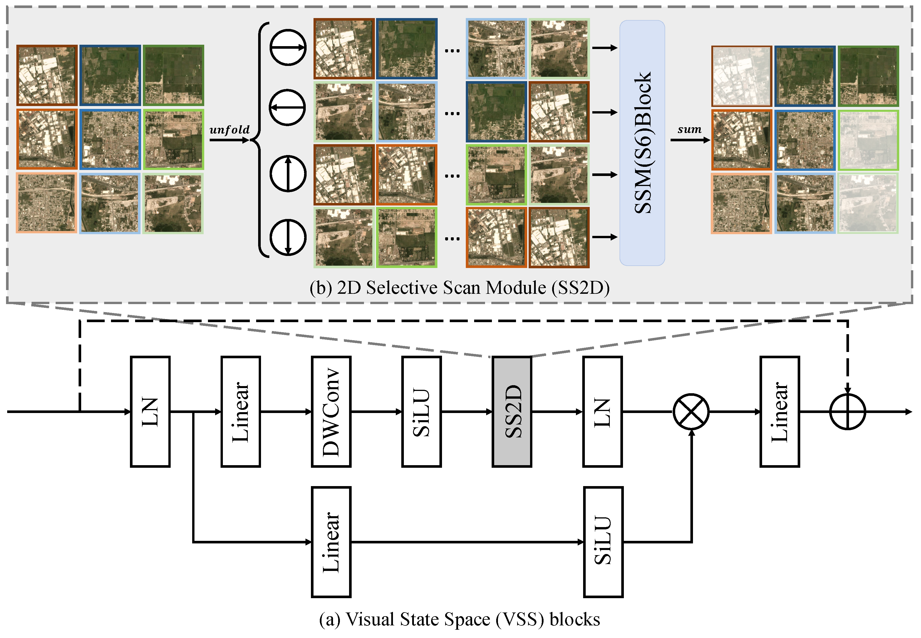
3.5. Spatial–Temporal Relationship Extraction Module

3.5.1. State Space Model

The State Space Model (SSM) offers a new method for globally processing contextual information. Inspired by linear time-invariant systems, it maps a one-dimensional (1-D) function or sequence $x\left(t\right)\in R$ to a response $y\left(t\right)\in R$ through a hidden state $h\left(t\right)\in R^N$. These systems are usually expressed as a set of linear ordinary differential equations (ODEs):

$$\begin{array}{cc}\hfill h^{\prime }\left(t\right)& =Ah\left(t\right)+Bx\left(t\right)\hfill \end{array}$$

(13)

$$\begin{array}{cc}\hfill y\left(t\right)& =Ch\left(t\right)\hfill \end{array}$$

(14)

where $A\in R^{N\times N}$, $B\in R^{N\times 1}$, and $C\in R^{1\times N}$ are system matrices, and $h\left(t\right)$ is the hidden state vector at time t. To accommodate the discrete nature of data in deep learning, Mamba provides a discrete representation of the continuous system. The zero-order hold (ZOH) method is used to convert the continuous parameters A and B into their discrete forms $\overline{A}$ and $\overline{B}$, as follows:

$$\begin{array}{cc}\hfill \overline{A}& =exp\left(\mathsf{\Delta }A\right)\hfill \end{array}$$

(15)

$$\begin{array}{cc}\hfill \overline{B}& ={\left(\mathsf{\Delta }A\right)}^{-1}\left(exp\left(\mathsf{\Delta }A\right)-I\right)\mathsf{\Delta }B\hfill \end{array}$$

(16)

where $\mathsf{\Delta }A=A\mathsf{\Delta }T$, $\mathsf{\Delta }B=B\mathsf{\Delta }T$, and $\mathsf{\Delta }T$ is the time step parameter. After discretization, continuous ODEs can be expressed as:

$$\begin{array}{cc}\hfill h_t^{\prime }& =\overline{A}{h}_{t-1}+\overline{B}{x}_t\hfill \end{array}$$

(17)

$$\begin{array}{cc}\hfill y_t& =C{h}_t\hfill \end{array}$$

(18)

In visual tasks, VMamba builds on Mamba’s selective scanning mechanism by introducing the Cross-Scan Module (CSM) [49]. This module enhances the model’s ability to extract spatio-temporal features from TSIs with temporal correlations, making it more effective for TSCD tasks.

3.5.2. Spatial-Temporal Relationship Extraction Module

In change detection tasks, understanding spatio-temporal relationships is crucial, as it involves the interdependence and changes in object categories across both time and space. Temporal relationships primarily capture dependencies between land cover classes at different time points, while spatial relationships focus on the dependencies between land cover classes and their surrounding areas at the same time. In TSIs, unchanged regions typically maintain consistent semantics over time, allowing temporal context to effectively integrate multi-temporal features. Land-cover changes often display strong spatial correlations. If changed pixels are spatially independent from their surroundings, they are likely to indicate pseudo-changes. By combining spatial and temporal relationships, we gain a comprehensive understanding of land cover change patterns, ultimately improving the accuracy of detection.

Visual State Space Block: The STREM is based on Mamba’s Visual State Space (VSS) Block, as shown in Figure 4a. The input is first passed through a layer normalization (LN) and then split into two branches. One branch goes through a linear layer followed by the Sigmoid Linear Unit (SiLU), while the other feeds the input into a sequence consisting of a linear transformation, depth-wise convolution (DWConv), and the SiLU activation function. The processed data are then directed to the 2D Selective Scan (SS2D) for context extraction. Afterward, the data pass through another LN and are merged with the output from the first branch, obtaining the final output of the VSS Block.

Specifically, the SS2D mechanism consists of three basic stages: an expansion operation, an S6 block for processing, and a scan merging operation. As shown in Figure 4b, the expansion stage rearranges tokens in the spatial dimension, moving them in four directions: from top left to bottom right, bottom right to top left, top right to bottom left, and bottom left to top right. These rearranged tokens are then fed into the S6 block, which scans information from each direction to extract comprehensive features. Finally, an addition operation merges global modeling information from multiple directions. The S6 block introduces a selective filter to dynamically adjust inputs by fine-tuning the parameters of the SSM, enabling the system to focus on relevant information and discard unnecessary details.

Spatial–Temporal Scanning Strategy: To effectively capture the spatial–temporal properties of images and model their relationships, we introduce two scanning strategies for the time dimension: the Spatial–Temporal Alternated Scan Strategy and the Spatial–Temporal Concatenated Scan Strategy. The Spatial–Temporal Alternated Scan Strategy sorts image features alternately at each time step, represented as ${\widehat{F}}_{\mathrm{alter}}=\left[f_1^l,f_2^l,\cdots ,f_T^l\right]$, where $l=1,2,3,4,5$. The Spatial–Temporal Concatenated Scan Strategy concatenates features along the channel dimension, shown as ${\widehat{F}}_{\mathrm{concat}}=\mathrm{concat}\left(f_1^l,f_2^l,\cdots ,f_T^l\right)$, with $l=1,2,3,4,5$, as illustrated in Figure 5. After being sorted by the two scanning strategies, the features are fed into the VSS Block for feature modeling, effectively capturing rich spatial–temporal relationships in the images.

STREBlock: As illustrated in Figure 5, for each layer l, alternated and concatenated features $F_{alter}^l$ and $F_{concat}^l$ are first mapped to a high-dimensional space using a $1\times 1$ convolution $Con{v}_{1\times 1}$. These processed features are then separately fed into the VSS Block to extract spatial–temporal feature, yielding $F_{sta}^l$ and $F_{stc}^l$. The extracted features are concatenated along the channel dimension with the corresponding level change feature $f_{cd}^l$ to form $F_{cat}^l$. Finally, another $1\times 1$ convolution $Con{v}_{1\times 1}$ is applied to $F_{cat}^l$ to unify the channel dimensions, producing the final output $F_o^l$. This process ensures effective spatial–temporal feature integration while maintaining dimensional consistency. The detailed process is as follows:

$$\begin{array}{cc}\hfill {\widehat{F}}_{alter}^l,{\widehat{F}}_{concat}^l& ={Conv}_{1\times 1}\left(F_{alter}^l\right),{Conv}_{1\times 1}\left(F_{concat}^l\right)\hfill \end{array}$$

(19)

$$\begin{array}{cc}\hfill F_{sta}^l,F_{stc}^l& =VSS\left({\widehat{F}}_{alter}^l\right),VSS\left({\widehat{F}}_{concat}^l\right)\hfill \end{array}$$

(20)

$$\begin{array}{cc}\hfill F_{cat}^l& =Concat(F_{sta}^l,F_{stc}^l,f_{cd}^l)\hfill \end{array}$$

(21)

$$\begin{array}{cc}\hfill F_o^l& ={Conv}_{1\times 1}\left(F_{cat}^l\right)\hfill \end{array}$$

(22)

STREM: The STREM consists of five STREBlocks, as shown in Figure 6. For each layer of the input sequence feature ${\left\{f_{seg}^l\right\}}_{l=1}^5$, spatio-temporal features are extracted using STREBlock. The resulting features are then concatenated with the corresponding change features $f_{cd}^l$ of the same scale l to form $F_{ST}^l$. The upsampled results $F_{ST}^{l-1}$ from the previous stage $l-1$ are then fused with $F_{ST}^l$. By processing each layer sequentially, the final fused change feature map $F_{fuse}^5$ is obtained, as described below:

$$\begin{array}{c}{F}_{ST}^l=STREBlock(F_{alter}^l,F_{concat}^l,f_{cd}^l)\end{array}$$

(23)

$$\begin{array}{c}{F}_{fuse}^l=ConvBlock(Up\left(F_{ST}^{l-1}\right)\oplus F_{ST}^l),l=2,3,4,5\end{array}$$

(24)

where Up(·) represents upsampling, ConvBlock includes convolution, batch normalization and ReLU, and ⊕ denotes addition.

3.6. Multi-Task Decoders

We apply two separate decoders to transform the segmentation and change feature maps into semantic and change outputs, respectively.

Semantic branch: For each layer l, feature information is fused using layer-by-layer deconvolution and skip connections to enhance the retention of feature details. Then, a semantic decoding head, implemented as a $1\times 1$ convolution layer, predicts pixel-level semantics. The process is as follows:

$$\begin{array}{c}{F}_{dec}^l=Concat(ConvT\left(f_{seg}^l\right),f_{seg}^{l-1}),l=2,3,4,5\end{array}$$

(25)

$$\begin{array}{c}{\widehat{y}}_{seg}=softmax\left({Conv}_{1\times 1}\left(f_{dec}^5\right)\right)\end{array}$$

(26)

where ConvT represents the transposed convolution, and ${\widehat{y}}_{seg}$ is the final output of semantic segmentation.

Change branch: The decoder predicts changes using $F_{fuse}^5$ from the STREM. This is processed through a change decoder head, a $1\times 1$ convolution layer, to generate the detection output as follows:

$$\begin{array}{c}{\widehat{y}}_{cd}=sigmoid\left({Conv}_{1\times 1}\left(F_{fuse}^5\right)\right)\end{array}$$

(27)

where ${\widehat{y}}_{cd}$ is the final output of change.

3.7. Loss Function

In the semantic branch, we utilize PowerJaccardLoss as the loss function, as follows:

$$\begin{array}{c}\hfill L_{sem}=\mathrm{PowerJaccardLoss}\left(y_n,{\widehat{y}}_n\right)\hfill \\ \hfill =1-\sum _{n=1}^{HW}{\displaystyle \frac{y_n·{\widehat{y}}_n}{\left(y_n^p{\widehat{y}}_n^p-y_n·{\widehat{y}}_n\right)+\epsilon }}\hfill \end{array}$$

(28)

where $y_n$ and ${\widehat{y}}_n$ represent the semantic ground truth and prediction results of each position n, respectively.

For the change branch, we employ the same loss function as the semantic branch, PowerJaccardLoss, which is expressed as:

$$\begin{array}{c}\hfill L_{cd}=\mathrm{PowerJaccardLoss}\left(y_n,{\widehat{y}}_n\right)\hfill \\ =1-\sum _{n=1}^{HW}{\displaystyle \frac{y_n·{\widehat{y}}_n}{\left(y_n^p{\widehat{y}}_n^p-y_n·{\widehat{y}}_n\right)+\epsilon }}\hfill \end{array}$$

(29)

where $y_n$ and ${\widehat{y}}_n$ represent the change ground truth and prediction results of each position n, respectively.

In addition, change detection tasks focus only on detecting changes while often ignoring semantic information. To address this, we introduce a loss function, $L_{cons}$, to supervise semantic consistency by aligning high-dimensional semantic features. This loss function implicitly guides the network’s learning by aligning the high-dimensional semantic feature representations of unchanged regions between the pre- and post-temporal images, thus making full use of the available sample information. Specifically, for the normalized bi-temporal features $d_1$ and $d_2$ after decoding, the semantic representations of unchanged regions should ideally be similar. We use cosine similarity to measure the similarity between the two, and $L_{cons}$ is defined as follows:

$$\begin{array}{c}\hfill L_{cons}=y·\left[1-\cos \left(d_1,d_2\right)\right]\end{array}$$

(30)

where y represents the ground truth for unchanged regions. The unchanged area label is 1, and the changed area is 0, which is used to exclude the changed area. The final loss function is

$$\begin{array}{c}\hfill L={\lambda }_1{L}_{sem}+{\lambda }_2{L}_{cd}+{\lambda }_3{L}_{cons}\end{array}$$

(31)

In this work, the weights of the above three losses were the same, with ${\lambda }_1$, ${\lambda }_2$, and ${\lambda }_3$ all set to 1.

4. Experiments and Results

4.1. Datasets

For our task, we used two datasets that provided continuous observation data of the same area, suitable for both training and evaluation.

SpaceNet7 dataset [50]: The SpaceNet7 dataset consists of TSIs from 60 global regions, collected by Planet Lab between 2017 and 2020. Each region includes 24 monthly images with a resolution of approximately 4 m and a size of $1024\times 1024$ pixels. The dataset features labels for two classes: buildings and non-buildings. We divided the dataset into training, testing, and validation sets in a 4:1:1 ratio. During training, two images from a randomly selected region are chosen as the pre-change and post-change images for change detection. These images, together with the preceding $N-2$ images from the pre-change period, form an image sequence of length N, while the validation and test sets consisted of N consecutive images from each region. Therefore, in our method, we focused on changes in buildings.

DynamicEarthNet dataset [51]: The DynamicEarthNet dataset includes images from 75 regions around the world, providing daily observations of unobstructed multispectral images over two consecutive years (2018–2019). Semantic segmentation labels are available for the first day of each month and cover categories such as impervious surfaces, water, soil, agriculture, wetlands, ice and snow, forests, and other vegetation. The dataset contains 54,750 satellite images and 1800 annotations, with each image containing four channels (RGB + near-infrared) at a resolution of 3 m and a size of $1024\times 1024$ pixels. We used only the images with available labels, selecting 35, 10, and 10 areas of interest (AOIs) for training, validation, and testing, respectively. The selection method for the training, validation, and test sets follows the same approach as SpaceNet7 dataset, with a one-month interval. In our experiments, we considered changes in all categories.

4.2. Evaluation Metrics

To assess the performance of the proposed model in TSCD, we employed four metrics: precision, recall, F1-score (F1), and Kappa coefficient (KP). These metrics are defined as follows:

$$\begin{array}{cc}PR\hfill & ={\displaystyle \frac{TP}{TP+FP}}\hfill \end{array}$$

(32)

$$\begin{array}{cc}RC\hfill & ={\displaystyle \frac{TP}{TP+FN}}\hfill \end{array}$$

(33)

$$\begin{array}{cc}F1\hfill & ={\displaystyle \frac{2\times PR\times RC}{PR+RC}}\hfill \end{array}$$

(34)

$$\begin{array}{cc}KP\hfill & ={\displaystyle \frac{OA-E}{1-E}}\hfill \end{array}$$

(35)

$$\begin{array}{cc}OA\hfill & ={\displaystyle \frac{TP+TN}{TP+TN+FP+FN}}\hfill \end{array}$$

(36)

$$\begin{array}{cc}E\hfill & ={\displaystyle \frac{\left(TP+FP\right)\times \left(TP+FN\right)+\left(FN+TN\right)\times \left(FP+TN\right)}{{\left(TP+TN+FP+FN\right)}^2}}\hfill \end{array}$$

(37)

where $TP$, $TN$, $FP$, and $FN$ represent the number of true positives, true negatives, false positives, and false negatives, respectively.

4.3. Experiment Settings

The proposed network was implemented using the PyTorch v1.12.0 framework. During training, we used the AdamW optimizer to update the network parameters, as it can adjust the learning rate and promote convergence. We set the number of image sequences N to 3, the initial learning rate to 0.0001, and the weight decay to 0.01. The training was run for 50 epochs with a batch size of eight. Data augmentation techniques such as horizontal and vertical flips and rotations $k\times {90}^{\circ },\mathrm{where}k\in \{1,2,3\}$ were applied. Training was conducted on an NVIDIA RTX A6000 GPU with 48 GB of memory, and the best result from the validation set over the 50 epochs was used for testing.

To alleviate the imbalance of positive and negative samples in the change detection task, we employed an importance sampling strategy to help the network focus on learning changes during training. Specifically, for any set of training samples, the change labels from images were randomly divided into 20 patches, each sized $256\times 256$. The probability of sampling each patch was determined by the proportion of changed pixels it contained. Additionally, to ensure that some unchanged areas were also included in the training, a baseline probability was assigned to regions with minimal or no changes. Each region was sampled 100 times.

4.4. Performance Comparison

In order to verify the effectiveness of the proposed method, we compared the following methods, which could be divided into two categories. One was the representative excellent bi-temporal change detection network, including FC-Siam-Diff [19], SNUNet [17], BIT [18], ChangeFormer [36], Changevit [52], SCanNet [53], MambaCD (Base/Small/Tiny) [54], RSMamba [55]; the other was the sequence detection method that integrates spatio-temporal information and can be used for multi-temporal change detection tasks, including ConvLSTM [56], L-UNet [15], MTL-UNet [57], U-TAE [58], Unet3D [59], and SitsSCD [60], as follows:

1.

FC-Siam-Diff [19]: a feature-level late fusion method that uses pseudo-Siamese FCN to extract and fuse bi-temporal multi-level features through feature difference operation.

2.

SNUNet [17]: uses a Siamese network as the encoder with shared parameters between the two branches. By incorporating the Ensemble Channel Attention Module (ECAM) in deep supervision, it naturally fuses shallow and deep features with semantic information, effectively reducing the semantic gap in deep supervision.

3.

BIT-CD [18]: a bi-temporal image transformer network that learns a compact set of tokens to reveal changes in interest in bi-temporal images, leveraging transformers to establish relationships between semantic concepts in the token-based space-time.

4.

Changevit [52]: a ViT-based framework that captures large-scale object information, complemented by a detail capture module for fine-grained features.

5.

ChangeFormer [36]: a Siamese network combining a hierarchically structured Transformer encoder with an MLP decoder to capture multi-scale, long-range details necessary for change detection.

6.

SCanNet [53]: a three-branch encoder–decoder network that learns semantic and change labels using concatenated image pairs and features, processed by an internal transformer to produce a binary change mask and semantic segmentation maps.

7.

RSMamba [55]: designed for dense prediction tasks in remote sensing, it uses an omnidirectional selective scanning module to globally model image context and capture features from all directions.

8.

MambaCD-Base/Small/Tiny [54]: uses the Mamba architecture to model global spatial and spatio-temporal relationships in multi-temporal images, with variations in the number of encoder layers and feature channels.

9.

ConvLSTM [56]: convolutional LSTM replaces the fully connected layer in traditional LSTM with a convolutional layer to exploit spatial information, enhancing long-term dependency capture in sequential data.

10.

L-UNet [15]: a UNet-like architecture that integrates ConvLSTM into its structure. In the decoding stage, ConvLSTM captures temporal relationships among TSIs. Its output is then passed to the decoder via a skip connection, enabling the fusion of temporal features at multiple scales.

11.

SitsSCD [60]: uses TSIs to handle semantic change detection, modifying the UTAE’s temporal attention mechanism to generate binary change maps and semantic segmentation maps for each image.

12.

MTL-UNet [57]: a fully convolutional LSTM network that models temporal relationships of spatial features, jointly learning construction extraction and change detection.

13.

Unet3D [59]: extends the UNet architecture with 3D convolution to simultaneously process spatial and temporal information for spatio-temporal feature modeling.

14.

U-TAE [58]: encodes temporal features in latent space through self-attention, leveraging multi-temporal remote sensing images to model temporal information. It uses a U-Net architecture with a Temporal Attention Encoder.

Numerically,

Table 1. Quantitative evaluation results on the SpaceNet7 and DynamicEarthNet datasets. The highest values are highlighted in red, and the second-highest in blue. All results are described in percentage (%).

Type	Method		SpaceNet7		DynamicEarthNet
			PR/RC/F1/KP		PR/RC/F1/KP
B	FC-Siam-Diff [19]		19.89/22.52/21.12/21.06		8.01/40.03/13.35/11.78
	SNUNet [17]		23.52/29.19/26.05/26.01		15.58/34.95/21.55/18.88
	BIT-CD [18]		17.04/23.00/19.58/19.53		58.39/11.12/18.68/10.67
	ChangeVit [52]		25.35/31.45/28.07/28.02		15.93/35.32/21.96/19.28
	ChangeFormer [36]		13.82/39.27/20.45/20.41		9.97/34.44/15.47/13.39
	SCanNet [53]		20.85/24.50/22.53/20.16		28.87/25.58/27.13/22.75
	RSMamba [55]		23.26/25.73/24.43/24.38		16.78/30.65/21.68/18.61
	MambaCD-Base [54]		22.39/34.13/27.04/27.00		16.76/32.64/22.15/19.22
	MambaCD-Small [54]		23.46/35.01/28.09/28.05		20.04/41.96/27.12/24.52
	MambaCD-Tiny [54]		26.06/30.00/27.89/27.85		12.33/42.74/19.14/17.16
M	ConvLSTM [56]		12.17/26.30/16.64/16.60		7.14/38.01/12.02/10.51
	L-UNet [15]		13.43/28.51/18.26/18.22		20.97/17.62/19.15/19.09
	SitsSCD [60]		19.29/10.95/13.97/13.89		18.37/14.57/16.25/10.95
	MTL-UNet [57]		20.97/17.62/19.15/19.09		10.52/36.89/16.37/14.34
	UNet3D [59]		24.31/26.24/25.24/25.19		22.41/28.40/25.05/21.35
	UTAE [58]		24.67/29.31/26.79/26.74		24.10/28.66/26.18/22.39
	Ours		28.88/39.01/33.19/33.14		28.20/33.89/30.78/27.25

presents the overall performance of all methods on the SpaceNet7 and DynamicEarthNet datasets. Here, B denotes bi-temporal methods, while M refers to multi-temporal methods.

Clearly, our method outperformed others in continuous bi-temporal change detection, surpassing both bi-temporal and multi-temporal change detection methods. Specifically, HiSTENet achieved a significant advantage across both datasets with its F1 surpassing the second-best method by 5.1% on the SpaceNet7 dataset and 3.65% on the DynamicEarthNet dataset. The Mamba-based method, which effectively utilizes spatio-temporal context information, achieved the second-highest PR, F1, and KP on the SpaceNet7 dataset. Although its F1 on the DynamicEarthNet dataset was slightly lower than the top two methods—by only 0.01%, it demonstrated the effectiveness of the Mamba architecture’s spatio-temporal information modeling and its potential in TSCD tasks. This also highlighted the superiority of our proposed STREM in spatio-temporal feature information extraction. Furthermore, while ChangFormer achieved the highest RC on SpaceNet7, it suffered from a low PR score. Similarly, BIT-CD attained the highest PR on DynamicEarthNet but had a lower RC, while Mamba-CD showed the best RC but a lower PR. Therefore, although our method did not excel in PR and RC individually, it struck the best balance between them, resulting in the highest F1 and KP. This analysis underscores the importance of integrating spatio-temporal and historical information in multi-temporal image change detection tasks, demonstrating its critical role in TSCD.

To further demonstrate the effectiveness of our proposed method, we conducted a qualitative analysis on the SpaceNet7 and DynamicEarthNet datasets, as shown in Figure 7 and Figure 8. In these figures, white pixels represent changed areas (TP), black pixels represent background (TN), blue pixels represent missed detections (FN), and red pixels highlight false positives (FP).

In the SpaceNet7 dataset, several representative samples were selected for visualization comparison. As shown in Figure 7a,b,d,e, some models exhibited more significant omissions, particularly in areas with similar features such as color and illumination. In contrast, our algorithm excelled at detecting small regions and areas with high similarity, providing more accurate edge detail predictions, which can be seen from Figure 7h,j.

Additionally, compared to the cases in Figure 7b,c, which were affected by differences in perspective and illumination, most other change detection models suffered from varying degrees of false detection. Our method, however, effectively handled sudden changes in the visual environment by incorporating temporal information, thereby reducing the false detection rate and achieving remarkably precise discrimination. This highlights the advantages of feature-aware alignment at both the channel and spatial levels.

It is worth noting that the SpaceNet7 dataset focuses primarily on building changes. To further evaluate the performance of change detection across multiple semantic categories, we also validated our method on the DynamicEarthNet dataset, which covers a broader range of land-cover types. Our method demonstrated superior visualization results. For example, in Figure 8b, our approach nearly matched the ground truth for large-area surface vegetation changes. In Figure 8c, where apparent color differences cause interference, our method outperformed BIT, SitsSCD, and others, showing no false detection due to this interference. This further underscores the robustness of HiSTENet against environmental disturbances.

It is evident that our network could accurately detect various types and quantities of changes under different conditions present in the image pairs, producing results that closely matched the reference change map. In summary, the qualitative analysis aligns with the quantitative results in Table 1, further confirming that the proposed HiSTENet achieves state-of-the-art performance on the SpaceNet7 and DynamicEarthNet datasets.

4.5. Ablation Experiments

To further assess the impact of each module on change detection performance, we conducted an ablation study using the SpaceNet7 and DynamicEarthNet datasets. The baseline model was defined as a U-Net structure as backbone for feature extraction (denoted as Baseline). As each module played a specific role within the framework, addressing specific tasks, and working collaboratively to enhance the overall performance of change detection, the following experiments were carried out to analyze and discuss the impact of adding different components: the Spatial–Temporal Relationship Extraction Module (denoted as STREM), the Historical Integration Module (denoted as HIM), the Feature Alignment and Fusion Module (denoted as FAFM) and a semantic consistency loss function (denoted as Loss). The evaluation focused on precision (PR), recall (RC), and F1-score, as shown in

Table 2. Ablation study on different components. The highest values are bolded in black.

Baseline	STREM	HIM	FAFM	Loss			SpaceNet7		DynamicEarthNet
							PR/RC/F1		PR/RC/F1
✔							27.88/30.13/28.96		24.98/28.04/26.42
✔	✔						27.67/35.31/31.02		28.73/31.50/30.05
✔		✔					29.78/30.97/30.36		31.50/24.37/27.48
✔			✔				24.98/35.57/29.35		25.01/29.30/26.98
✔				✔			26.10/34.10/29.57		27.67/26.50/27.07
✔	✔	✔					28.33/35.12/31.36		29.52/27.78/28.63
✔	✔	✔	✔				26.08/40.62/31.77		30.18/28.96/29.56
✔	✔	✔	✔	✔			28.88/39.01/33.19		28.02/33.89/30.78

,

Table 3. Ablation study on different strategies in STREM. The highest values are bolded in black.

Model	AS	CS			SpaceNet7		DynamicEarthNet
					PR/RC/F1		PR/RC/F1
HiSTENet					26.06/32.69/29.00		31.05/28.05/29.48
HiSTENet		✔			29.02/31.60/30.25		27.79/32.70/30.05
HiSTENet	✔				30.96/29.73/30.33		32.71/28.02/30.18
HiSTENet	✔	✔			28.88/39.01/33.19		28.02/33.89/30.78

and

Table 4. Ablation study on different features in HIM. The highest values are bolded in black.

Model	All	Unique			SpaceNet7		DynamicEarthNet
					PR/RC/F1		PR/RC/F1
HiSTENet					26.17/33.31/29.31		31.05/28.05/29.47
HiSTENet	✔				27.95/32.63/30.11		31.62/27.92/29.66
HiSTENet		✔			28.88/39.01/33.19		28.02/33.89/30.78

and Figure 9.

Effects of different components in HiSTENet: To validate the effectiveness of the key modules in the proposed HiSTENet, ablation experiments were conducted, as shown in Table 2. The results revealed that although some precision or recall values were lower than the baseline when the key modules were added individually or in different combinations, the F1-score achieved a better balance, with a final increase of 4.23% and 4.36% over the baseline. And as shown in Figure 9, the baseline (I) exhibited incomplete edge detection and noticeable false negatives, indicating its limited ability to capture change information. With the addition of the STREM (II), which primarily incorporates spatio-temporal information, more details of the change regions were captured, reducing false negatives. However, some false positives remained due to the increased sensitivity. By further integrating the HIM (III), which fuses historical information through feature interaction, an improvement in detection performance and edge completeness could be observed. This demonstrates the effectiveness of incorporating richer information in enhancing change detection. When the FAFM was introduced (IV), the model became more capable of distinguishing between change and non-change regions, leading to a reduction in false negatives. However, a slight increase in false positives was observed due to the model’s enhanced sensitivity. Finally, the full HiSTRENet (V) achieved the best balance between precision and recall, effectively addressing incomplete edges and false negatives while minimizing excessive false positives. These experiments demonstrate that the proposed method achieves a better trade-off between false positives and false negatives, enhancing the overall change detection performance.

Effects of different strategies of STREM: The proposed STREM effectively exploits spatio-temporal correlations in multi-temporal images using Alternated Scanning (AS) and Concatenated Scanning (CS) extraction strategies. By modeling spatio-temporal features and incorporating them into the semantic and change feature fusion process, the module improved the F1-score by 2.06% and 3.63%, demonstrating its effectiveness. Since the STREM focuses on modeling spatio-temporal relationships, it may better capture change regions and improve recall. However, it might also introduce more false positives, leading to a decrease in precision. By adjusting the weight of spatio-temporal information, the strength of modeling can be balanced to avoid over-capturing irrelevant regions.

To further investigate the impact of different spatio-temporal feature extraction strategies on experimental results, we conducted a series of experiments, as shown in Table 3. “AS” refers to the Alternated Scan Strategy and “CS” refers to the Concatenated Scan Strategy. It can be observed that AS significantly improved recall, while CS had a greater impact on precision. There was no noticeable difference in the improvement of the F1-score when applied individually, but the combination of both strategies produced a more significant enhancement. This indicates that the features extracted by “AS” and “CS” are complementary, and their combination creates a synergistic effect that significantly enhances the model’s overall performance.

Effects of HIM: The proposed HIM integrates historical image feature information through feature interaction. The experimental results shown in Table 2 demonstrate that HIM effectively enhanced the feature representation of the images, mitigating misdetections and missed detections caused by interference. This improvement led to a 1.40% and 1.06% increase in the F1-score, thereby enhancing the accuracy of the detection results.

Additionally, experiments were conducted to evaluate different feature selection methods. The “All” method used all historical features for enhancement and “Unique” method utilized only unchanged historical features. As shown in Table 4, the inclusion of historical image information enriched feature details, allowing the model to learn visual features under different imaging conditions, thus improving detection accuracy. Among these methods, using only unchanged features outperformed using all features. This can be attributed to the fact that while using the full set of features introduces more detailed information, it also introduces noise related to changes. By focusing only on unchanged features, the model effectively reduces interference and achieves superior detection outcomes.

Effects of FAFM: The FAFM enables the network to capture the offsets between the dual-temporal images, addressing local mismatches through resampling and alignment operations. The experimental results in Table 2 show that the introduction of the FAFM increased the F1-score by 0.39% and 0.56%, confirming the effectiveness of the proposed module in reducing the impact of pseudo-changes. During the process of correcting registration errors, the FAFM may misclassify some unchanged regions as changed ones due to insufficient generalization ability in feature alignment, which can be mitigated by introducing additional constraints on low-confidence regions to reduce false positives.

Effects of semantic consistency learning: To fully utilize semantic labels, we designed a loss function that supervised semantic consistency learning by aligning high-dimensional semantic features. This function implicitly guided the network by aligning semantic feature representations of pre- and post-temporal images. It effectively addressed the imbalance between positive and negative samples, enhancing semantic consistency in unchanged areas. This approach improved the F1-score by 0.61% and 0.65%, and strengthened the model’s robustness, which is shown in Table 2. Semantic features of unchanged regions may vary naturally (e.g., due to lighting or perspective changes), so the loss function should incorporate a relaxation mechanism to avoid overly strict constraints.

4.6. Computational Efficiency

In general, the number of parameters (Params.), inference time (Time), and floating-point operations (FLOPs) are three critical factors for evaluating the computational efficiency of deep models. Among these, FLOPs provide a direct measure of a model’s computational complexity, determined by the input image size and neural network architecture.

Table 5. Computational efficiency, including the total number of the floating-point operations (FLOPs), the total number of the parameters (Params.) and the total time of inference (Time) and in the model. The F1-scores calculated on SpaceNet7 and DynamicEarthNet datasets are also listed here for comparison.

Type	Method	FLOPs (G)	Params. (M)	Time (s)	F1 (%)
B	FC-Siam-Diff [19]	4.73	1.35	0.067497	21.12/13.35
	SNUNet [17]	54.83	12.03	0.030320	26.05/21.55
	BIT-CD [18]	10.61	3.50	0.057397	19.58/18.68
	ChangeVit [52]	38.81	32.14	0.082682	28.07/21.96
	ChangeFormer [36]	202.79	41.03	0.102586	20.45/15.47
	SCanNet [53]	66.23	27.90	0.056208	22.53/27.13
	RSMamba [55]	18.33	42.30	0.136785	24.43/21.68
	MambaCD-Base [54]	44.83	85.53	0.419819	27.04/22.15
	MambaCD-Small [54]	28.7	49.94	0.183827	28.09/27.12
	MambaCD-Tiny [54]	17.54	27.54	0.130364	27.89/19.14
M	ConvLSTM [56]	60.71	0.31	0.008655	16.64/12.02
	L-Unet [15]	30.57	8.45	0.195141	18.26/19.15
	SitsSCD [60]	854.68	16.16	0.088565	13.97/16.25
	MTL-UNet [57]	48.89	9.43	0.215808	19.15/16.37
	UNet3D [59]	26.99	0.34	0.023896	25.24/25.05
	UTAE [58]	40.9	1.08	0.281565	26.79/26.18
	Ours	156.57	17.62	0.184011	33.19/30.78

presents an analysis of these factors for our model. We assessed inference time and efficiency using $256\times 256$ pixel image pairs, with experiments conducted on a single NVIDIA RTX 6000 Ada GPU (NVIDIA Corporation, Santa Clara, CA, USA) with 48 GB of memory.

From the comparison of parameter count (Params.) and computational complexity (FLOPs) in Table 5, it is evident that our model maintained excellent performance while keeping computational overhead relatively moderate. Our model had 17.62 M parameters and 156.57 G FLOPs, which was in the mid-to-high range among all models. Its F1 score was 33.19% on SpaceNet7 and 30.78% on DynamicEarthNet, the best among all models. In contrast, the BIT-CD and ConvLSTM methods had the lowest parameter counts, at 3.50 M and 0.31 M, respectively, indicating their extremely low computational cost. However, despite their low computational load, their performance in practical applications was subpar, with BIT-CD scoring 19.58% and 18.68% on two datasets, and ConvLSTM scoring 16.64% and 12.02%. MambaCD-Tiny and SNUNet offered a good balance between computational cost and performance. MambaCD-Tiny had 17.54 G FLOPs and 27.54 M parameters, achieving F1 scores of 27.89% and 19.14%. SNUNet, with 54.83 G FLOPs and 12.03 M parameters, scored 26.05% and 21.55%. ChangeFormer had a much higher computational load than the MambaCD series and BIT-CD, but its performance was mediocre. Despite its high computational cost, its lower F1 scores indicated that it did not achieve the expected detection results under high computational load.

Regarding inference time, there were significant differences among the models: BIT-CD and ConvLSTM had the shortest inference times but also the lowest F1 scores. ChangeFormer and our model were more complex models with longer inference times. MambaCD-Base and MambaCD-Tiny had relatively fast inference speeds and reasonable F1 scores. Our model achieved a good balance between inference time, parameter count, and FLOPs, while also excelling in performance and efficiency. Higher FLOPs generally correlate with longer training times due to the larger amount of computation required per iteration. FC-Siam-Diff, with only 4.73 G FLOPs, had the shortest training time. BIT-CD and ConvLSTM, among other methods, used moderate training times. ChangeFormer and our method had the highest FLOPs, at 202.79 G and 156.57 G, respectively, resulting in the longest training times, but they also achieved the highest F1 scores. The proposed model achieved an ideal balance between performance and computational efficiency, demonstrating its ability to deliver the best performance with reasonable resources. However, its relatively high FLOPs and parameter count may pose challenges in resource-constrained environments. In contrast, MambaCD-Tiny and SNUNet offered good performance with lower computational costs, making them suitable for scenarios requiring a balance between resources, training time, and performance. During the experiment on SpaceNet7, we recorded the training time of each model and found that ConvLSTM was the fastest, completing training in 1 h 21 min 50 s. This is likely due to its lightweight architecture, though it came at the cost of lower performance. Mamba-Tiny followed with a training time of 2 h 10 min 03 s, possibly benefiting from the linear scanning mechanism of Mamba-based models, which accelerates the training process. The slowest model, UTAE, took 6 h 40 min 40 s, likely due to its use of temporal self-attention at each layer, which reduces computational efficiency. Our proposed method achieved a balanced performance, completing training in 4 h 46 min 35 s, effectively leveraging Mamba’s efficiency while maintaining a moderate training time.

Notably, when processing a large number of TSIs, the historical image information can be directly reused for current-time change detection, enhancing processing speed and response efficiency, albeit with some memory trade-offs. Additionally, the smaller parameter count compared to more complex networks highlights the lightweight nature of the proposed method, reducing the risk of overfitting. They confirm the computational efficiency and practicality of HiSTENet, underscoring its potential for real-time applications.

5. Discussion

In summary, our experimental results demonstrated that the proposed HiSTENet achieved outstanding performance on the SpaceNet7 and DynamicEarthNet datasets. It not only surpassed classical BTCD methods but also outperformed many TSCD methods, highlighting its significant practical application value and great potential for future development. We attribute its success to four key aspects of the model design:

1.

We designed the STREM to model the spatio-temporal features of image sequences, enabling our method to comprehensively reference both temporal and spatial dimensions, thereby better capturing change information.

2.

The HIM effectively and efficiently integrates features from historical images, allowing the model to better understand the attributes of objects under varying imaging conditions, thus enhancing its ability to recognize changes in interest.

3.

By applying the FAFM to learn and correct pixel shifts in the feature space for the image pairs being analyzed, the model mitigates the occurrence of pseudo-changes caused by local mismatches.

4.

The introduction of a semantic consistency loss helps address the issue of imbalance between positive and negative samples in change detection datasets, improving the stability of model training.

However, the proposed HiSTENet also has several limitations that need to be addressed in future work:

1.

Simplistic feature selection for historical images: The feature selection process for historical images is relatively simple, relying only on randomly generated hard labels and focusing solely on unchanged regions during feature exchange. This approach heavily depends on ground-truth labels and fails to fully exploit the potential information and contextual relationships in the data. Such a random feature selection strategy does not make the most of the available information. Therefore, future research could explore the incorporation of temporal attention mechanisms to enable adaptive selection and utilization of important features. This would enhance the model’s understanding of temporal changes, allowing it to more accurately extract critical information from historical images for change detection tasks.

2.

Limited feature exchange for multi-modal data: The current feature exchange process only handles homologous features, which works well for single-mode data but struggles with multi-modal data. Multi-modal datasets often involve information from different sensors or sources, with significant differences in feature distribution, scale, and semantics. To address this, future research could focus on unifying feature representations across modalities by introducing cross-modal feature alignment techniques or modality-adaptive modules, enhancing the model’s ability to handle multi-modal data.

6. Conclusions

In this paper, we proposed HiSTENet, a new method for TSCD. It effectively used spatial-temporal and object features to achieve accurate change detection. The HIM enhanced multi-temporal image features through selective feature exchange, highlighting the representation capability of the visual features in change regions and improving their effectiveness in decoding stage. The FAFM then aligned spatial offsets between bi-temporal images, reducing pseudo-changes and generating accurate multi-scale change features. Meanwhile, the STREM used scanning strategies to extract spatial-temporal features from images, integrating them with FAFM-processed features to enhance temporal perception and produce high-quality predictions. Evaluations on the SpaceNet7 and DynamicEarthNet datasets showed that the HiSTENet surpassed existing methods, achieving F1/Kappa scores of 33.19%/33.14% and 30.78%/27.25% and demonstrating strong generalization and robustness. Looking forward, the TSCD field may benefit from the development of more generalizable models and the integration of multi-modal data sources. Future work will aim to improve historical image use, enrich the data utilized, and enhance the model’s generalization capabilities to extend its applicability to broader and more diverse remote sensing tasks.

References

1. Singh, A. Review article digital change detection techniques using remotely-sensed data. Int. J. Remote Sens. 1989, 10, 989–1003. [Google Scholar] [CrossRef]
2. Wan, L.; Tian, Y.; Kang, W.; Ma, L. D-TNet: Category-awareness based difference-threshold alternative learning network for remote sensing image change detection. IEEE Trans. Geosci. Remote Sens. 2022, 60, 5633316. [Google Scholar] [CrossRef]
3. Liu, C.; Zhao, R.; Chen, J.; Qi, Z.; Zou, Z.; Shi, Z. A Decoupling Paradigm with Prompt Learning for Remote Sensing Image Change Captioning. IEEE Trans. Geosci. Remote Sens. 2023, 61, 5622018. [Google Scholar] [CrossRef]
4. Wan, L.; Tian, Y.; Kang, W.; Ma, L. CLDRNet: A Difference Refinement Network based on Category Context Learning for Remote Sensing Image Change Detection. IEEE J. Sel. Top. Appl. Earth Obs. Remote. Sens. 2023, 17, 2133–2148. [Google Scholar] [CrossRef]
5. Giustarini, L.; Hostache, R.; Matgen, P.; Schumann, G.J.P.; Bates, P.D.; Mason, D.C. A Change Detection Approach to Flood Mapping in Urban Areas Using TerraSAR-X. IEEE Trans. Geosci. Remote Sens. 2013, 51, 2417–2430. [Google Scholar] [CrossRef]
6. Bovolo, F.; Bruzzone, L. A Split-Based Approach to Unsupervised Change Detection in Large-Size Multitemporal Images: Application to Tsunami-Damage Assessment. IEEE Trans. Geosci. Remote Sens. 2007, 45, 1658–1670. [Google Scholar] [CrossRef]
7. Gupta, R.; Goodman, B.; Patel, N.N.; Hosfelt, R.; Sajeev, S.; Heim, E.T.; Doshi, J.; Lucas, K.; Choset, H.; Gaston, M.E. xBD: A Dataset for Assessing Building Damage from Satellite Imagery. arXiv 2019, arXiv:1911.09296. [Google Scholar]
8. Willis, K.S. Remote sensing change detection for ecological monitoring in United States protected areas. Biol. Conserv. 2015, 182, 233–242. [Google Scholar] [CrossRef]
9. Ji, R.; Tan, K.; Wang, X.; Pan, C.; Xin, L. Spatiotemporal Monitoring of a Grassland Ecosystem and Its Net Primary Production Using Google Earth Engine: A Case Study of Inner Mongolia from 2000 to 2020. Remote Sens. 2021, 13, 4480. [Google Scholar] [CrossRef]
10. Zhu, Z.; Qiu, S.; Ye, S. Remote sensing of land change: A multifaceted perspective. Remote Sens. Environ. 2022, 282, 113266. [Google Scholar] [CrossRef]
11. Li, J.; Wu, C. Using difference features effectively: A multi-task network for exploring change areas and change moments in time series remote sensing images. ISPRS J. Photogramm. Remote Sens. 2024, 218, 487–505. [Google Scholar] [CrossRef]
12. Verbesselt, J.; Hyndman, R.; Zeileis, A.; Culvenor, D. Phenological change detection while accounting for abrupt and gradual trends in satellite image time series. Remote Sens. Environ. 2010, 114, 2970–2980. [Google Scholar] [CrossRef]
13. Kennedy, R.E.; Yang, Z.; Cohen, W.B. Detecting trends in forest disturbance and recovery using yearly Landsat time series: 1. LandTrendr—Temporal segmentation algorithms. Remote Sens. Environ. 2010, 114, 2897–2910. [Google Scholar] [CrossRef]
14. Zhu, Z.; Woodcock, C.E. Continuous change detection and classification of land cover using all available Landsat data. Remote Sens. Environ. 2014, 144, 152–171. [Google Scholar] [CrossRef]
15. Sun, S.; Mu, L.; Wang, L.; Liu, P. L-UNet: An LSTM Network for Remote Sensing Image Change Detection. IEEE Geosci. Remote Sens. Lett. 2022, 19, 8004505. [Google Scholar] [CrossRef]
16. Li, J.; Hu, M.; Wu, C. Multiscale change detection network based on channel attention and fully convolutional BiLSTM for medium-resolution remote sensing imagery. IEEE J. Sel. Top. Appl. Earth Obs. Remote. Sens. 2023, 16, 9735–9748. [Google Scholar] [CrossRef]
17. Fang, S.; Li, K.; Shao, J.; Li, Z. SNUNet-CD: A Densely Connected Siamese Network for Change Detection of VHR Images. IEEE Geosci. Remote. Sens. Lett. 2021, 19, 8007805. [Google Scholar] [CrossRef]
18. Chen, H.; Qi, Z.; Shi, Z. Remote sensing image change detection with transformers. IEEE Trans. Geosci. Remote Sens. 2021, 60, 5607514. [Google Scholar] [CrossRef]
19. Daudt, R.C.; Le Saux, B.; Boulch, A. Fully convolutional siamese networks for change detection. In Proceedings of the 2018 25th IEEE International Conference on Image Processing (ICIP), Athens, Greece, 7–10 October 2018; pp. 4063–4067. [Google Scholar]
20. Xiao, W.; Cao, H.; Lei, Y.; Zhu, Q.; Chen, N. Cross-temporal and spatial information fusion for multi-task building change detection using multi-temporal optical imagery. Int. J. Appl. Earth Obs. Geoinf. 2024, 132, 104075. [Google Scholar] [CrossRef]
21. Wang, L.; Zhang, J.; Bruzzone, L. MixCDNet: A Lightweight Change Detection Network Mixing Features across CNN and Transformer. IEEE Trans. Geosci. Remote. Sens. 2024, 62, 4411915. [Google Scholar] [CrossRef]
22. He, L.; Zhang, M.; Li, Y.; Zhang, J.; Luo, S.; Li, S.; Zhang, X. Change-Guided Similarity Pyramid Network for Semantic Change Detection. IEEE Trans. Geosci. Remote. Sens. 2024, 62, 5637917. [Google Scholar] [CrossRef]
23. Ren, W.; Wang, Z.; Xia, M.; Lin, H. MFINet: Multi-scale feature interaction network for change detection of high-resolution remote sensing images. Remote Sens. 2024, 16, 1269. [Google Scholar] [CrossRef]
24. Gu, A. Modeling Sequences with Structured State Spaces. Ph.D Thesis, Stanford University, Stanford, CA, USA, 2023. [Google Scholar]
25. Gu, A.; Dao, T. Mamba: Linear-time sequence modeling with selective state spaces. arXiv 2023, arXiv:2312.00752. [Google Scholar]
26. Chen, J.; Chen, X.; Cui, X.; Chen, J. Change Vector Analysis in Posterior Probability Space: A New Method for Land Cover Change Detection. IEEE Geosci. Remote Sens. Lett. 2011, 8, 317–321. [Google Scholar] [CrossRef]
27. Mu, C.; Huo, L.; Liu, Y.; Liu, R.; Jiao, L. Change detection for remote sensing images based on wavelet fusion and PCA-kernel fuzzy clustering. Acta Electron. Sin 2015, 43, 1375–1381. [Google Scholar]
28. Daudt, R.C.; Saux, B.L.; Boulch, A.; Gousseau, Y. Urban Change Detection for Multispectral Earth Observation Using Convolutional Neural Networks. In Proceedings of the IGARSS 2018—2018 IEEE International Geoscience and Remote Sensing Symposium, Valencia, Spain, 22–27 July 2018. [Google Scholar]
29. Ronneberger, O.; Fischer, P.; Brox, T. U-Net: Convolutional Networks for Biomedical Image Segmentation. In Proceedings of the International Conference on Medical Image Computing and Computer-Assisted Intervention, Munich, Germany, 5–9 October 2015. [Google Scholar]
30. Badrinarayanan, V.; Kendall, A.; Cipolla, R. SegNet: A Deep Convolutional Encoder-Decoder Architecture for Image Segmentation. IEEE Trans. Pattern Anal. Mach. Intell. 2017, 39, 2481–2495. [Google Scholar] [CrossRef]
31. Basavaraju, K.S.; Sravya, N.; Lal, S.; Nalini, J.; Reddy, C.S.; Dell’Acqua, F. UCDNet: A Deep Learning Model for Urban Change Detection From Bi-Temporal Multispectral Sentinel-2 Satellite Images. IEEE Trans. Geosci. Remote Sens. 2022, 60, 5408110. [Google Scholar] [CrossRef]
32. Pang, S.; Zhang, A.; Hao, J.; Liu, F.; Chen, J. SCA-CDNet: A robust siamese correlation-and-attention-based change detection network for bitemporal VHR images. Int. J. Remote. Sens. 2021, 43, 6102–6123. [Google Scholar] [CrossRef]
33. Jian, P.; Chen, K.; Cheng, W. Gan-based one-class classification for remote-sensing image change detection. IEEE Geosci. Remote Sens. Lett. 2021, 19, 8009505. [Google Scholar] [CrossRef]
34. Alexey, D. An image is worth 16x16 words: Transformers for image recognition at scale. arXiv 2020, arXiv:2010.11929. [Google Scholar]
35. Shi, N.; Chen, K.; Zhou, G. A divided spatial and temporal context network for remote sensing change detection. IEEE J. Sel. Top. Appl. Earth Obs. Remote Sens. 2022, 15, 4897–4908. [Google Scholar] [CrossRef]
36. Bandara, W.G.C.; Patel, V.M. A transformer-based siamese network for change detection. In Proceedings of the IGARSS 2022—2022 IEEE International Geoscience and Remote Sensing Symposium, Kuala Lumpur, Malaysia, 17–22 July 2022; pp. 207–210. [Google Scholar]
37. Feng, J.; Yang, X.; Gu, Z. SGNet: A Transformer-Based Semantic-Guided Network for Building Change Detection. IEEE J. Sel. Top. Appl. Earth Obs. Remote. Sens. 2024, 17, 9922–9935. [Google Scholar] [CrossRef]
38. Zhang, Z.; Fan, X.; Wang, X.; Qin, Y.; Xia, J. A Novel Remote Sensing Image Change Detection Approach Based on Multi-level State Space Model. IEEE Trans. Geosci. Remote. Sens. 2024, 62, 4417014. [Google Scholar] [CrossRef]
39. Wang, H.; Ye, Z.; Xu, C.; Mei, L.; Lei, C.; Wang, D. TTMGNet: Tree Topology Mamba-Guided Network Collaborative Hierarchical Incremental Aggregation for Change Detection. Remote Sens. 2024, 16, 4068. [Google Scholar] [CrossRef]
40. Hochreiter, S.; Schmidhuber, J. Long short-term memory. Neural Comput. 1997, 9, 1735–1780. [Google Scholar] [CrossRef]
41. Saha, S.; Bovolo, F.; Bruzzone, L. Change detection in image time-series using unsupervised LSTM. IEEE Geosci. Remote Sens. Lett. 2020, 19, 8005205. [Google Scholar] [CrossRef]
42. Kalinicheva, E.; Ienco, D.; Sublime, J.; Trocan, M. Unsupervised change detection analysis in satellite image time series using deep learning combined with graph-based approaches. IEEE J. Sel. Top. Appl. Earth Obs. Remote Sens. 2020, 13, 1450–1466. [Google Scholar] [CrossRef]
43. Yang, B.; Qin, L.; Liu, J.; Liu, X. UTRNet: An unsupervised time-distance-guided convolutional recurrent network for change detection in irregularly collected images. IEEE Trans. Geosci. Remote Sens. 2022, 60, 4410516. [Google Scholar] [CrossRef]
44. Yang, B.; Qin, L.; Liu, J.; Liu, X. IRCNN: An irregular-time-distanced recurrent convolutional neural network for change detection in satellite time series. IEEE Geosci. Remote Sens. Lett. 2022, 19, 2503905. [Google Scholar] [CrossRef]
45. Meshkini, K.; Bovolo, F.; Bruzzone, L. An unsupervised change detection approach for dense satellite image time series using 3d cnn. In Proceedings of the 2021 IEEE International Geoscience and Remote Sensing Symposium IGARSS, Brussels, Belgium, 12–16 July 2021; pp. 4336–4339. [Google Scholar]
46. Meshkini, K.; Bovolo, F.; Bruzzone, L. Multi-Annual Change Detection Using a Weakly Supervised 3D CNN in HR SITS. IEEE Geosci. Remote. Sens. Lett. 2024, 21, 5001405. [Google Scholar] [CrossRef]
47. Fang, S.; Li, K.; Li, Z. Changer: Feature Interaction is What You Need for Change Detection. IEEE Trans. Geosci. Remote Sens. 2023, 61, 5610111. [Google Scholar] [CrossRef]
48. Dai, J.; Qi, H.; Xiong, Y.; Li, Y.; Zhang, G.; Hu, H.; Wei, Y. Deformable convolutional networks. In Proceedings of the IEEE International Conference on Computer Vision, Venice, Italy, 27–29 October 2017; pp. 764–773. [Google Scholar]
49. Liu, Y.; Tian, Y.; Zhao, Y.; Yu, H.; Xie, L.; Wang, Y.; Ye, Q.; Liu, Y. VMamba: Visual State Space Model. arXiv 2024, arXiv:2401.10166. [Google Scholar]
50. Van Etten, A.; Hogan, D.; Manso, J.M.; Shermeyer, J.; Weir, N.; Lewis, R. The multi-temporal urban development spacenet dataset. In Proceedings of the IEEE/CVF Conference on Computer Vision and Pattern Recognition, Nashville, TN, USA, 20–25 June 2021; pp. 6398–6407. [Google Scholar]
51. Toker, A.; Kondmann, L.; Weber, M.; Eisenberger, M.; Camero, A.; Hu, J.; Hoderlein, A.P.; Şenaras, Ç.; Davis, T.; Cremers, D.; et al. Dynamicearthnet: Daily multi-spectral satellite dataset for semantic change segmentation. In Proceedings of the IEEE/CVF Conference on Computer Vision and Pattern Recognition, New Orleans, LA, USA, 18–24 June 2022; pp. 21158–21167. [Google Scholar]
52. Zhu, D.; Huang, X.; Huang, H.; Shao, Z.; Cheng, Q. ChangeViT: Unleashing Plain Vision Transformers for Change Detection. arXiv 2024, arXiv:2406.12847. [Google Scholar]
53. Ding, L.; Zhang, J.; Guo, H.; Zhang, K.; Liu, B.; Bruzzone, L. Joint spatio-temporal modeling for semantic change detection in remote sensing images. IEEE Trans. Geosci. Remote. Sens. 2024, 62, 5610814. [Google Scholar] [CrossRef]
54. Chen, H.; Song, J.; Han, C.; Xia, J.; Yokoya, N. Changemamba: Remote sensing change detection with spatio-temporal state space model. arXiv 2024, arXiv:2404.03425. [Google Scholar]
55. Zhao, S.; Chen, H.; Zhang, X.; Xiao, P.; Bai, L.; Ouyang, W. Rs-mamba for large remote sensing image dense prediction. arXiv 2024, arXiv:2404.02668. [Google Scholar] [CrossRef]
56. Shi, X.; Chen, Z.; Wang, H.; Yeung, D.Y.; Wong, W.K.; Woo, W.c. Convolutional LSTM network: A machine learning approach for precipitation nowcasting. Adv. Neural Inf. Process. Syst. 2015, 28, 802–810. [Google Scholar]
57. Papadomanolaki, M.; Vakalopoulou, M.; Karantzalos, K. A deep multitask learning framework coupling semantic segmentation and fully convolutional LSTM networks for urban change detection. IEEE Trans. Geosci. Remote Sens. 2021, 59, 7651–7668. [Google Scholar] [CrossRef]
58. Garnot, V.S.F.; Landrieu, L. Panoptic segmentation of satellite image time series with convolutional temporal attention networks. In Proceedings of the IEEE/CVF International Conference on Computer Vision, Montreal, BC, Canada, 11–17 October 2021; pp. 4872–4881. [Google Scholar]
59. M Rustowicz, R.; Cheong, R.; Wang, L.; Ermon, S.; Burke, M.; Lobell, D. Semantic segmentation of crop type in Africa: A novel dataset and analysis of deep learning methods. In Proceedings of the IEEE/CVF Conference on Computer Vision and Pattern Recognition Workshops, Long Beach, CA, USA, 16–17 June 2019; pp. 75–82. [Google Scholar]
60. Vincent, E.; Ponce, J.; Aubry, M. Satellite Image Time Series Semantic Change Detection: Novel Architecture and Analysis of Domain Shift. arXiv 2024, arXiv:2407.07616. [Google Scholar]
Figure 1. Overview of proposed History-Integrated Spatial-Temporal Information Extraction Network.
Remotesensing 17 00792 g001
Figure 2. The architecture of the Historical Integration Module.
Remotesensing 17 00792 g002
Figure 3. Illustration of the Feature Alignment and Fusion Module.
Remotesensing 17 00792 g003
Figure 4. Illustration of VSSBlock with the 2D Selective Scanning (SS2D) mechanism. (a) Description of VSSBlock. (b) The detailed structure of the SS2D mechanism.
Remotesensing 17 00792 g004
Figure 5. Architecture of STREBlock. The red arrows indicate the scanning direction.
Remotesensing 17 00792 g005
Figure 6. The architecture of the Spatial–Temporal Relationship Extraction Module.
Remotesensing 17 00792 g006
Figure 7. Qualitative evaluation results on the SpaceNet7 dataset. (ah) are some examples. (i) and (j) are magnified views of the red boxes in (c) and (e), respectively.
Remotesensing 17 00792 g007
Figure 8. Qualitative evaluation results on the DynamicEarthNet dataset. (ah) are some examples. (i) and (j) are magnified views of the red boxes in (d) and (g), respectively.
Remotesensing 17 00792 g008
Figure 9. Some examples of the qualitative results from the ablation study. The first and second columns are the images of the two input temporal. (I) is the Baseline, (II) is Baseline+STREM, (III) is Baseline+STREM+HIM, (IV) is Baseline+STREM+HIM+FAFM and (V) is HiSTRENet.
Remotesensing 17 00792 g009