Accuracy Evaluation of Multi-Technique Combination Nonlinear Terrestrial Reference Frame and EOP Based on Singular Spectrum Analysis

Abstract

With the application and promotion of space geodesy, the popularization of remote sensing technology, and the development of artificial intelligence, a more accurate and stable Terrestrial Reference Frame (TRF) has become more urgent. For example, sea level change detection, crustal deformation monitoring, and driverless cars, among others, require the accuracy of the terrestrial reference frame to be better than 1 mm in positioning and 0.1 mm/a in velocity, respectively. However, the current frequently used ITRF2014 and ITRF2020 do not satisfy such requirements. Therefore, this paper analyzes the coordinate residual time series data of linear TRFs and finds there are still some unlabeled jumps and time-dependent periodic signals, especially in the GNSS coordinate residuals, which can lead to incorrect station epoch coordinates and velocities, further affecting the accuracy and stability of the TRF. The unlabeled jumps could be detected by the sequential t-test analysis of regime shifts (STARS) combined with the generalized extreme Studentized deviate (GESD) algorithms introduced in our earlier paper. These nonlinear time-dependent periodic signals could be modeled better by singular spectrum analysis (SSA) with respect to least squares fitting; the fitting period is no longer composed of semi-annual and annual items, as with ITRF2014. The periods of continuous coordinate residual time series data longer than 5 years are obtained by FFT. The results show that there are no period signals for individual SLR/VLBI sites, and there are still other period terms, such as 34 weeks, 20.8 weeks and 17.3 weeks, in addition to semi-annual and annual items for some GNSS sites. Moreover, after SSA corrections, the re-calculated TRF and the corresponding EOP could be obtained, based on data from the Chinese Earth Rotation and Reference System Service (CERS) TRF and the Earth Orientation Parameter (EOPs) multi-technique determination software package (CERS TRF&EOP V2.0) developed by the Shanghai Astronomical Observatory (SHAO). Their accuracy could be evaluated with respect to the ITRF2014 and the IERS 14 C04, respectively. The results show that the accuracy and stability of the newly established a nonlinear TRF and EOP based on SSA have been greatly improved and better than a linear TRF and EOP. SSA is better than least squares fitting, especially for those coordinate residual time series with varying amplitude and phase. For GPS, comparing with the ITRF2014, the station coordinate accuracy of 10.8% is better than 1 mm, and the station velocity accuracy of 4.4% is better than 0.1 mm/year. There are 3.1% VLBI stations, for which coordinate accuracy is better than 1 mm and velocity accuracy is better than 0.1 mm/year. However, there are no stations with coordinates and velocities better than 1 mm and 0.1 mm/year for the SLR and DORIS. The WRMS values of polar motion x, polar motion y, LOD, and UT1-UTC are reduced by 2.4%, 3.2%, 2.7%, and 0.96%, respectively. The EOP’s accuracy in SOL-B, in addition to LOD, is better than that of the JPL.

1. Introduction

Geokinetics, Earth rotation, and the gravity field are the three main research branches of space geodesy, and they are all strongly related to terrestrial reference frames (TRFs) [1,2]. The TRFs and EOPs (Earth orientation parameters) which describe the Earth rotation are determined by the 4 space geodesy techniques, including satellite laser ranging (SLR), global navigation satellite systems (GNSS), very long baseline interferometry (VLBI), and the Doppler orbitography and radio-positioning integrated by satellites (DORIS) [2,3,4,5]. The accuracy and stability of the TRFs are required to be 1 mm and 0.1 mm/year, respectively [2]. The TRF is a specific implementation of the terrestrial reference system (TRS). It consists of a set of specific terrestrial reference frame points on the Earth’s surface, including the coordinates and velocities of globally distributed space geodetic stations [2,6]. The TRF not only provides important references for classical geodesy, modern satellite navigation positioning, and precise orbit determination, but provides basic data for plate motion, crustal deformation, global/regional sea level change, land water, and glacier change, among other functions [2,3,4,5,6,7].

At present, the most accurate and widely used TRF is the International Terrestrial Reference Frame (ITRF). It was established and maintained by the International Earth Rotation Service (IERS) based on four types of space geodetic observations techniques [2,5,7]. It has been developed into a global millimeter level TRF [2]. In addition to the Institut national de l’information géographique et forestière (IGN), which is responsible for ITRF, two other organizations, the Deutsches Geodätisches Forschungsinstitut der Technischen Universität München (DGFI-TUM) and the Jet Propulsion Laboratory (JPL), have also established combined TRFs, named the DTRF and JTRF, respectively [2,8,9]. China has also been developing a global combined TRF, named the STRF, and an EOP time series, named the CERS (Chinese Earth Rotation and Reference System Service) EOP since 2014 [4].

Linear motion of stations due to factors such as plates tectonic motions, and crustal deformation is the dominant component in geodetic observations [10]. However, it is also very important to research the nonlinear motion of the stations due to seismic and volcanic activity, thermal expansion effects caused by temperature changes, non-tidal ocean loading, atmospheric loading, hydrological changes, and other geophysical processes [11,12,13,14]. Now, station nonlinear motions are considered in the determination of the TRF and the EOP [15]. For example, in the ITRF2014, Altamimi et al. empirically estimated seasonal periodic terms for all stations, which captures atmospheric loading as well as other aspects for the same periods [2,13]. The ITRF2014 was determined by long-term frame stacking [2], and the post-seismic deformation (PSD) model was used to optimize the internal model and to improve accuracy [2]. Wu et al. utilized the Kalman filter and backward smoother approaches to realize a nonlinear TRF, named JTRF2014, by synthesizing SLR/GNSS/VLBI/DORIS data at the JPL [9]. It solved the mismatch problems between the complex time-varying characteristics of crustal deformation and a long-term linear TRF [9]. Seitz et al. realized a nonlinear TRF considering atmospheric and hydrological non-tidal loading corrections, namely the DTRF2014 [8]. The Root Mean Square (RMS) values of the transformation between the DTRF2014 and the ITRF2014 show very small values [2,8,15], for the station positions, the RMS values are below 0.6 mm for GNSS and VLBI, and are below 2.3 mm for SLR and DORIS [2,8]. It shows the two TRFs are consistent [8]. Currently, the ITRF2020 is the most authoritative and the latest terrestrial reference frame, which is mainly determined by VLBI, SLR, GNSS (GPS, GLONASS, Galileo), and DORIS. Compared to the ITF2014, it has several improvements: consistency of velocity and seasonal signals at local tie between different technologies; the annual and semi-annual terms of the coordinates of stations with enough time span are estimated; and eight periodic signals are also considered for some stations. The core strategy of the DGFI is to synthesize the unconstrained equations established for various technologies [16,17], whose latest version is the DTRF2020, and take into account the non-tidal load and post-earthquake deformation models including atmosphere, hydrology, and ocean. The JPL uses square root filtering and the Dyer–McReynolds covariance smoothing method to implement the latest terrestrial reference frame, the JTRF2020 [18].

In China, He et al. introduced a weighted method of variance component estimation to solve the linear TRF, namely the STRF2014 and the consistent CERS EOP time series based on SLR/GNSS/VLBI/DORIS data with the information of global collocation sites [4]. However, in this implemented linear terrestrial reference frames, the time-varying amplitude periodic signals caused by the station’s nonlinear motion are not fully considered. The seasonal variation of the station coordinates resulting from climate changes and post-glacial rebound, among other variables is often time-varying. With the requirements of a high-precision TRF and EOP, these periodic signals need to be considered and modeled. Therefore, in this paper, based on the previous research (the linear STRF), we introduce singular spectrum analysis (SSA) to fit the periodic signals of the time-variable amplitude and establish a nonlinear model for GPS sites. Before SSA processing, missing data, gross error, and unlabeled jumps need to be processed. Then, based on the preprocessed GPS time series measurements, we apply SSA to extract periodic signals and reconstruct a nonlinear TRF and EOP. Finally, we evaluate the nonlinear STRF and EOP.

2. Methodology

2.1. Singular Spectrum Analysis

SSA was proposed by Broomhead et al. (1986) and was initially used to process meteorological data [19]. It was implemented by diagonalizing the corresponding empirical covariance matrix [19]. It is a data-driven method which can extract information from short and noisy time series data by applying time-domain data without a prior knowledge [19,20]. An important feature of SSA is that nonlinear variations can be detected [21,22]. The algorithm can be found in the literature [19,20,21,22,23].

For a coordinate residual time series $X=\left\{x_1,x_2,\dots ,x_N\right\}$, by sliding a time window of length $M$, the time series matrix is reconstructed into a new sequence, and the $k$-th component of the station coordinate residual sequence can be generated, the formula is as follows [22]:

$$x_i^k=\left\{\begin{array}{c}{\displaystyle \frac{1}{i}}{\displaystyle {\displaystyle \sum }_{j=1}^i}{a}_{i-j}^k{E}_j^k,\hspace{1em} 1\le i\le M-1 \\ {\displaystyle \frac{1}{M}}{\displaystyle {\displaystyle \sum }_{j=1}^M}{a}_{i-j}^k{E}_j^k,\hspace{1em} M\le i\le N-M+1\\ {\displaystyle \frac{1}{N-i+1}}{\displaystyle {\displaystyle \sum }_{j=i-N-M}^M}{a}_{i-j}^k{E}_j^k,\hspace{1em} N-M+2\le i\le N\end{array}\right.$$

(1)

where the eigenvector $E^k$ of the covariance matrix, $k=1,2,\dots ,M$;

$$a_i^k={\displaystyle \sum }_{j=1}^M{x}_{i+j}{E}_j^k 0\le i\le N-M$$

The SSA method can decompose the original time series and extract the top K components with significant contributions, then reconstructs the original sequence. This article uses the SSA method to identify and extract periodic terms from GPS station coordinate time series. According to the principle of SSA, when a periodic component exists in the original sequence, SSA will obtain a pair of reconstructed components (RCs), whose eigenvalues are close to equal and their corresponding T-EOF (known as temporal empirical orthogonal function) and T-PCs (known as temporal principal components) are orthogonal [22]. This method determines the selected component for sequence reconstruction and extracts the variable amplitude periodic signal.

Moreover, the lag-window size $M$ is a key factor for the SSA algorithm [22]. According to Vautard et al., $M$ should neither be too large nor too small [23]. Rangelova et al. applied a three-year window (156 weeks) to retrieve long-term changes together with seasonal variations from time series data [24]. Chen et al. applied a two-year window to extract annual and semi-annual signals from weekly GPS time series and confirmed that a window size of two or three years is appropriate [20]. Therefore, in this work, for the weekly GPS time series, we use two years (104 weeks) as $M$.

2.2. Least Squares Fitting

Least squares fitting is widely applied to weekly GPS time series to fit both linear and periodic terms. However, long periodic variations can be mistakenly identified as a linear trend when using the least-squares fitting method [20,24]. Coordinates of one station at one time epoch $t_i$, can be expressed as Equation (2).

$$\mathrm{y}\left(t_i\right)=h_0+v{t}_i+{\displaystyle \sum }_{j=1}^n[a_{j}sin\left(2\pi f_j{t}_i\right)+b_{j}cos\left(2\pi f_j{t}_i\right)]+\delta \left(t_i\right)$$

(2)

where $t_i$ is the epoch of observation, $h_0$ is a constant term, $v$ is the station velocity, $a_j$ and $b_j$ are the coefficients of periodic terms, $f_j$ is the periodic frequencies, and $\delta \left(t_i\right)$ is the noise term.

3. Time-Varying Periodic Signal Extraction

3.1. Data

In this paper, time series coordinates at GPS sites are calculated using the CERS TRF and EOP multi-technique determination software package (CERS TRF&EOP version 2.0), which was independently developed by the Shanghai Astronomical Observatory (SHAO) of the Chinese Academy of Sciences [4]. The input SINEX files are from ILRS, IGS, IVS, and IDS, with a similar length of the ITRF2014 [2]. The SLR SINEX files are from 1983 to 2015 provided by ILRS/ASI. The GNSS SINEX files used in the ITRF2014 or this paper is only from GPS system due to data length and data processing accuracy of other navigation systems. They are from 1997 to 2015 and are provided by the IGS/NRCan. The VLBI SINEX files are from 1980 to 2015 and are provided by the IVS/GIUB. The IDS SINEX files are from 1993 to 2015 and are provided by the IDS/IGN. Applying the SSA requires a fixed sampling interval and a temporal span of the time series data at least twice the lag-window width (M) [20]. Previous research has suggested a 2–3 years lag-window to extract annual and semi-annual periodic terms from the weekly GPS time series [20,24,25]. This means that data length of at least 5–6 years is necessary. Therefore, we choose a lag-window of 104 weeks for periodic terms, the data missing less than 15%, and the data length more than 5 years for reliable results.

3.2. Data Preprocessing

The GPS/SLR/VLBI/DORIS coordinate residual data was analyzed and it was found that there are significant period signals for most of GPS sites, but it is not so obvious for some SLR/VLBI/DORIS sites. The reasons may be a result from the time resolution of data, data continuity, data processing errors, geophysical factors, and so on. GPS has a better time resolution and data continuity than other techniques. It makes it easier for those period signals to be extracted. Due to the continuity and good time resolution, GPS is more sensitive to the period geophysical signals. Here, we just show the GPS SSA analysis results. Other techniques or other navigation systems are similar. The adopted method is the same.

Before SSA, the coordinate residual time series of the GPS stations needs to be preprocessed to tackle gross errors, data missing, trend items, station discontinuities, etc. [26,27,28]. Due to the SSA algorithm, it can only be applied to complete and equal interval sampling data. Therefore, interpolation of missing data is necessary after removing gross error. Jumps in space geodetic observations can be attributed to several reasons, such as geophysical phenomena (e.g., earthquakes), signal loss of the equipment, and so on [28,29]. These jumps cause discontinuities in the time series coordinates and lead to errors in the constructed TRF [29,30,31]. The sequential t-test analysis of regime shifts (STARS) algorithm is an effective method for detecting jumps in a GPS time series [32,33,34].

In this paper, before SSA, we perform data preprocessing including missing data, gross error, interpolation, and unlabeled jumps detection. We use the same discontinuities data as that used for the ITRF2014 first. But there are still some jumps in the coordinate residual time series after the establishment of the TRF. So, we call these jumps unlabeled jumps. These unlabeled jumps must be detected because they not only could affect the fitting of velocity but could affect the extraction of periodic terms. The discontinuities are a kind of similar linear signal. We usually extract period signals after de-linearization. This means discontinuities affect period extraction. The periodic signals in the station coordinate residual time series are more prominent after eliminating jumps. We have detected them by the sequential t-test analysis of regime shifts (STARS) method combined with the generalized extreme Studentized deviate (GESD) algorithm [35], which was introduced in our earlier paper [36]. After that, we introduced these discontinuities into the jump information file and then continued the establishment of the TRF. As a result, the station discontinuities have been repaired very well and the periodic signals in the station coordinate residual time series are more prominent. See our earlier paper [36].

3.3. Comparison of Least Squares Fitting and SSA

The least-squares fitting and SSA algorithms are tested in terms of their capability to extract periodic signals. A comparison between these two results is shown in Figure 1. Generally, the SSA method performs better than the least-squares fitting method. Figure 1a displays the coordinate variation along the X direction at CHUM. It demonstrates an obvious periodic change with varying amplitude and phase from 2002 to 2006. Compared with the SSA results (shown in the red line), the periodic signals derived by the least-squares fitting method (shown in the blue line) are of constant amplitude and phase. The least-squares fitting method shows an overfitting effect around the peaks. On the contrary, the fitting results of the SSA method follows closer to the signal peaks. Coordinate variations along the Y direction at the CHUM station are shown in Figure 1b, in which both results at the CHUM station display the periodic signals with almost constant amplitude and phase. Figure 1c illustrates coordinate variation along the Z direction at the CHUM station and the SSA method performs better than the least-squares fitting method in terms of matching the original signals.

3.4. SSA Results

By applying SSA, different scales of periodic components of the GPS time series can be identified and extracted, as seen in Figure 2, which shows the X coordinates variation of the SYDN station, the Y coordinates variation of the CHUM station, and the Z coordinates variation of the DRAO station. The reason why the different stations are used instead of one station is only to show more results of different sites. The time varying amplitude signals do not only exist in individual GPS sites. The stations selected in this article are intended to illustrate the applicability of the SSA method. The results of other stations or other directions are similar. The green lines represent the original time series and the black lines represent the extracted periodic signals in Figure 2(a1,b1,c1). Apart from annual and semi-annual components, periodic components of 34 weeks, 20.8 weeks, and 17.3 weeks are identified too. These periodic components are removed from the original time series, the results are shown in Figure 2(a2,b2,c2). The RMS values after removing the periodic components are reduced from 3.2494 mm to 1.8669 mm, which is decreased by 42.5%. For the CHUM and DRAO sites, they are decreased by 48.0% and 39.4%, respectively. However, nonlinear long-period terms caused by unknown geophysical factors may still remain, particularly evident in Figure 2(c2). Further study with more data in the future is required. Moreover, there are no period signals for individual SLR/VLBI sites. In short, SSA could improve the site coordinates accuracy, but it has high requirements for data length and data integrity which makes it necessary to select the station data in advance. This also means not all GNSS or GPS data are suitable for such SSA analysis.

4. Establishment of a Nonlinear Terrestrial Reference Frame and EOP Based on SSA

Two groups of GPS time series data could be generated with and without correction of periodic components by SSA. They are then combined with SLR/VLBI/DORIS SINEX files to determinate the TRF and EOP based on the CERS TRF&EOP multi-technique determination software package developed by SHAO. The linear STRF2014 and nonlinear STRF2014 solutions could be obtained, named SOL-A and SOL-B, respectively. The two solutions are evaluated for these aspects: TRF datum, station coordinates/velocity, and EOP results.

4.1. The Result Analysis of Datum Definition

The origin of the STRF is uniquely determined by SLR and the scale is also determined by both SLR and VLBI. Here, we firstly analyze and compare the translation parameter (x-/y-/z-translation) and scale time series of a linear STRF solution (SOL-A) and a nonlinear STRF solution (SOL-B). The results are shown in Figure 3 and Figure 4, which show the translation parameters of the time series and the scale of the linear/nonlinear STRF are very coincident. For the nonlinear STRF solution, the scale factor has a linear trend with k = −0.0221 ppb/yr relative to the SLR weekly solutions and a linear trend with k = 0.0013 ppb/yr relative to the VLBI 24-h solutions, which indicates that there is no significant linear difference between them.

The WRMS values of the translation parameters (x-/y-/z-translation) and the scale for the linear and nonlinear solutions are statistically analyzed and given in

Table 1. WRMS Values of translation parameters and scale from SOL-A and SOL-B.

Datum Parameters	WRMS
	SOL-A	SOL-B
X-component (mm)	4.2890	4.2600
Y-component (mm)	4.3400	4.3370
Z-component (mm)	7.4360	7.4350
Scale SLR (ppb)	0.8480	0.8110
Scale VLBI (ppb)	1.1250	1.0931

. It shows that the WRMS value of the X direction component of the translation parameters changes from 4.29 mm to 4.26 mm, which is decreased by 0.68%. The accuracy of the Y and the Z direction components are slightly improved and the WRMS values are reduced by 0.07% and 0.01%, respectively. The WRMS of scale is reduced by 4.3% and 2.8% relative to SLR and VLBI, respectively. After introducing into periodic components and recalculating, the stability of the translation and scale are improved, but it is not very obvious. This may be because the periodic signal’s extraction and processing are mainly applied to GPS data, which are not used in the determination of datum definition.

4.2. Accuracy Evaluation of Coordinates and Velocities

In this section, coordinates and velocities at GPS, SLR, VLBI, and DORIS sites derived by the two solutions (SOL-A and SOL-B) are compared with the ITRF2014, respectively. The results statistics and comparisons between linear/nonlinear STRF and the ITRF2014 are based on all stations. The differential values are divided into seven accuracy levels, accuracy better than 1 mm, accuracy at 1–2 mm, 2–3 mm, 3–5 mm, 5–10 mm, 10–20 mm, and accuracy worse than 20 mm. The evaluation is performed by counting the number of stations within each accuracy level. The statistic comparisons for GPS, SLR, VLBI, and DORIS are shown in Figure 5, Figure 6, Figure 7 and Figure 8, respectively.

Table 2. Statistics of coordinate and velocity accuracies for GPS/VLBI/SLR/DORIS sites in the nonlinear TRF SOL-B.

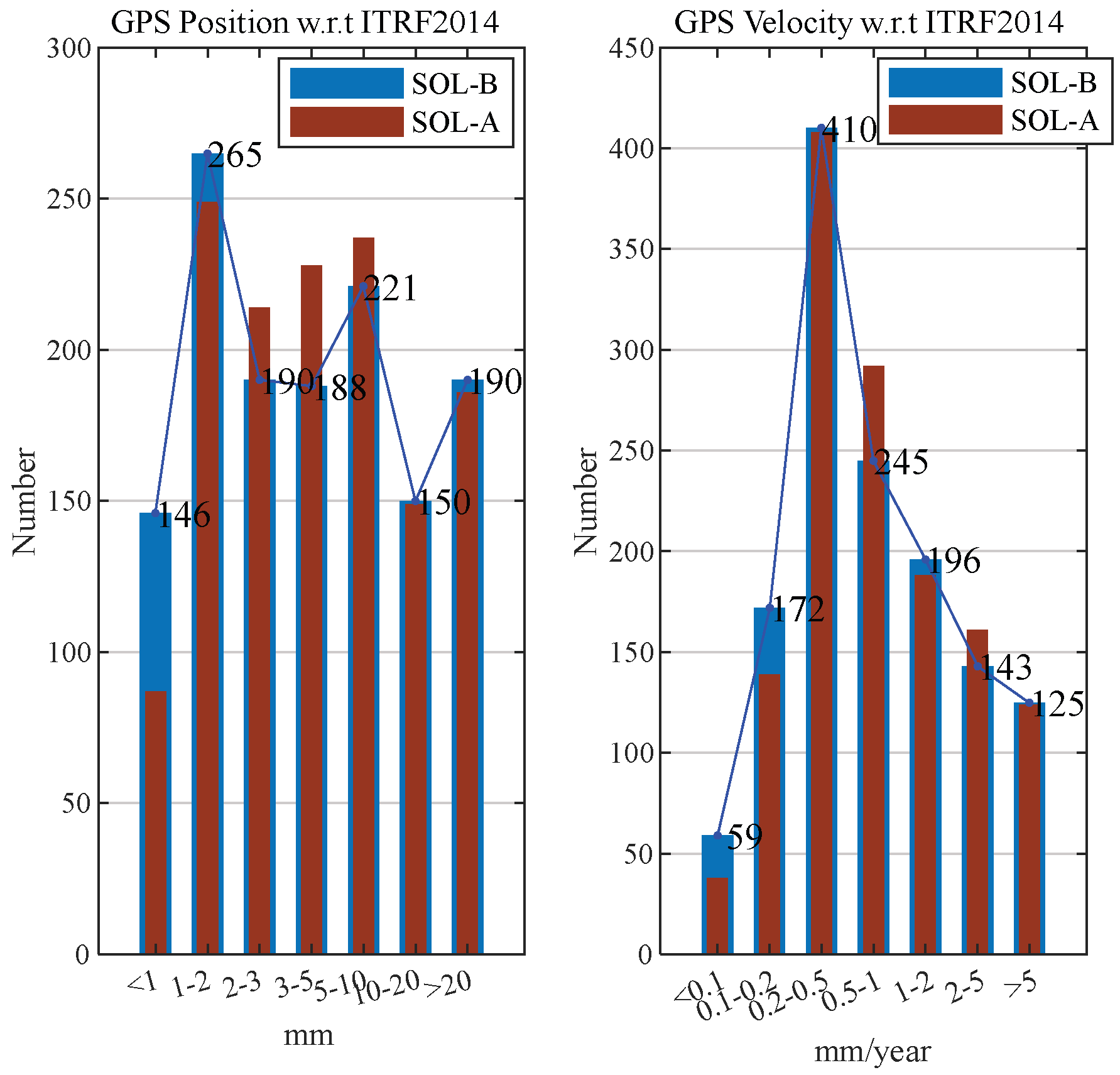
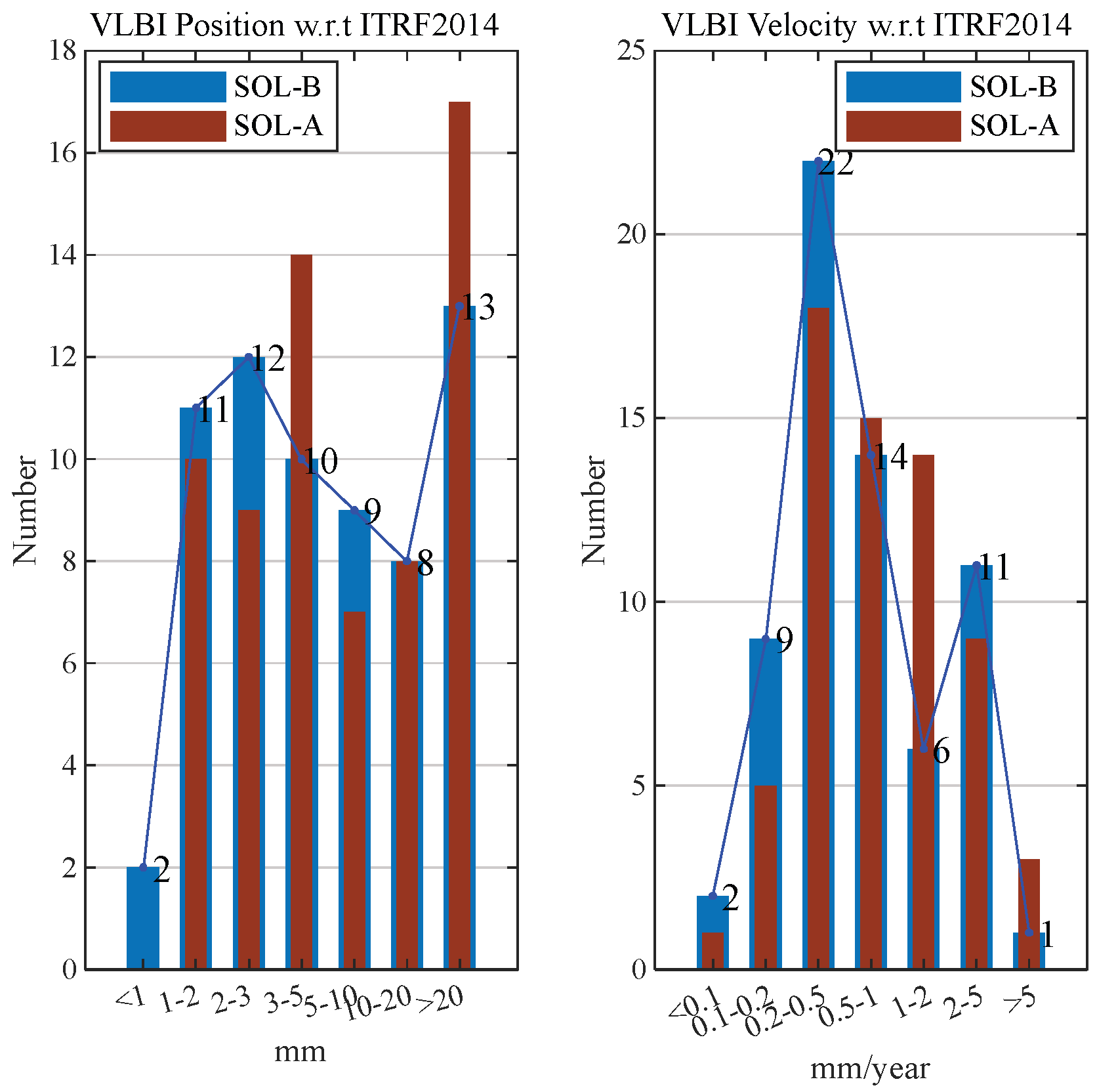
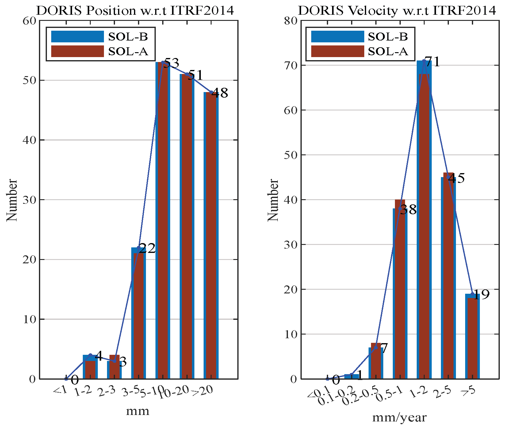
Coordinate Accuracy Level (mm)	Percentage of Stations (%)				Velocity Accuracy Level (mm/year)	Percentage of Stations (%)
	GPS	VLBI	SLR	DORIS		GPS	VLBI	SLR	DORIS
<1	10.8	3.1	0	0	<0.1	4.4	3.1	0	0
(1, 2)	19.6	16.9	1.6	2.2	(0.1, 0.2)	12.7	13.8	0	0.6
(2, 3)	14.1	18.5	5.6	1.7	(0.2, 0.5)	30.4	33.8	11.3	3.9
(3, 5)	13.9	15.4	9.7	12.2	(0.5, 1)	18.1	21.5	27.4	21.0
(5, 10)	16.4	13.8	18.5	29.3	(1, 2)	14.5	9.2	12.9	39.1
(10, 20)	11.1	12.3	19.4	28.2	(2, 5)	10.6	16.9	25.0	24.9
>20	14.1	20.0	45.1	26.5	>5	9.3	1.5	23.4	10.5

lists the percentage of statistical results of GPS/VLBI/SLR/DORIS sites coordinates and velocities compared with the ITRF2014.

In Figure 5, it can be seen that the nonlinear STRF (SOL-B) performs better than the linear STRF (SOL-A). More GPS stations are distributed in the high-precision, and fewer GPS stations are distributed in the lower-precision. There are 10.8% of the GPS stations with coordinate accuracy better than 1 mm and 4.4% of the GPS stations with a velocity accuracy better than 0.1 mm/year. There are 44.5% of the GPS stations with coordinate accuracy better than 3 mm and 47.5% of the GPS stations with a velocity accuracy better than 0.5 mm/year.

From Figure 6, Figure 7 and Figure 8, it is also obvious that the SOL-B performs better than the SOL-A. There are 3.1% of the VLBI stations with coordinate accuracy better than 1 mm and the same percentage stations with a velocity accuracy better than 0.1 mm/year. However, there are no stations with coordinates and velocities better than 1 mm and 0.1 mm/year for the SLR and DORIS stations. There are 7.2% and 3.9% of the total stations with a coordinate accuracy better than 3 mm, and 11.3% and 4.5% with velocity accuracy better than 0.5 mm/year for SOL-B and SOL-A, respectively. By comparison, DORIS results display a lower accuracy. We can conclude that the accuracy of the nonlinear TRF has been improved by considering the periodic signals extracted from SSA.

4.3. EOP Result Comparison and Analysis

The CERS TRF&EOP multi-technique determination software package not only calculates the TRF, but it calculates the EOP as well. Therefore, the corresponding EOP could be calculated with the nonlinear TRF based on SSA too. We choose the IERS 14 C04 as the reference to examine the accuracy of the EOP of SOL-A and SOL-B. Figure 9 displays the differences between the IERS 14 C04 and the EOPs of SOL-A and SOL-B. These two EOPs are basically consistent and have no significant deviation with respect to the IERS 14 C04.

Table 3. WRMS values of the EOP of SOL-A/SOL-B and the JPL with respect to the IERS 14 C04 EOP.

EOP Parameters	WRMS
	SOL-A	SOL-B	JPL EOP
x-component of Polar Motion (mas)	0.0578	0.0564	1.8540
y-component of Polar Motion (mas)	0.0595	0.0576	3.1290
UT1-UTC (ms)	0.0104	0.0103	0.0295
LOD (ms)	0.0112	0.0109	0.0049

shows the WRMS value of the EOP for SOL-A and SOL-B taking the IERS 14 C04 EOP as the reference. The accuracies of the polar motion, UT1-UTC, and LOD have been improved after introducing the periodic signals. The WRMS values of the LOD change from 0.0112 ms to 0.0109 ms with a decrease of 2.7%. The WRMS values of the x component, y component of polar motion and UT1-UTC have been decreased by 2.4%, 3.2%, and 0.96%, respectively. The accuracy of the EOP has improved and the detailed results are shown in Table 3.

At the same time, we compare the EOP of SOL-B with the JPL EOP, and still select the IERS 14 C04 EOP as the reference to evaluate the accuracy of the EOP of SOL-B and the JPL EOP. The results are shown in Figure 10. It illustrates that the accuracy of the polar motion and UT1-UTC in SOL-B is better than that of the JPL. Table 3 also displays the WRMS value of the JPL EOP with respect to the IERS 14 C04 EOP. The WRMS values of the polar motion and UT1-UTC in SOL-B are smaller than that of the JPL. It is mainly because the error of early data processing is large in the JPL. However, the accuracy of LOD in the JPL EOP is higher than that of SOL-B, and its WRMS value is 0.0049 ms. The early data processing for LOD is good.

5. Conclusions

This paper mainly focuses on the periodic component extraction based on SSA, the establishment of a nonlinear TRF and EOP, and their accuracy evaluation. Firstly, the singular spectrum analysis (SSA) method is introduced to fit and extract the periodic components of a coordinate residual time series derived by four space geodesy techniques, especially derived by GPS. Then, we use the self-developed CERS TRF&EOP multi-technique determination software package to recalculate the TRF and EOP and obtain the nonlinear TRF and its corresponding EOP. Finally, compared with the ITRF2014 and the IERS 14 C04 EOP, they are evaluated to obtain their accuracy.

We find that SSA is better than least squares fitting, especially for those coordinate residual time series with varying amplitude and phase. Compared with the SOL-A, the stability of translation parameters and scale in the SOL-B have been improved. The accuracy of the SOL-B is significantly higher than that of the SOL-A. For GPS, compared with the ITRF2014, 10.8% of the station coordinate accuracy is better than 1 mm, 4.4% of the station velocity accuracy is better than 0.1 mm/year. There are 3.1% of the VLBI stations with coordinate accuracy better than 1 mm and velocity accuracy better than 0.1 mm/year. However, there are no stations with coordinates and velocities better than 1 mm and 0.1 mm/year for SLR and DORIS. The accuracy of the EOP demonstrates that the accuracy of polar motion x, polar motion y, LOD, and UT1-UTC are all improved. Their WRMS values are reduced by 2.4%, 3.2%, 2.7%, and 0.96%, respectively. The accuracy of the EOP in the SOL-B, in addition to LOD, are better than that of the JPL. The SSA method is also suitable for comparison and analysis under the ITRF2020.

References

- Song, S.; Zhu, W.; Xiong, F.; Gao, J. Construction of mm-level terrestrial reference frame. Chin. J. Geophys. 2009, 52, 2704–2711. [Google Scholar]
- Altamimi, Z.; Rebischung, P.; Métivier, L.; Collilieux, X. ITRF2014: A new release of the international terrestrial reference frame modeling non-linear station motions. J. Geophys. Res. Solid Earth 2016, 121, 6109–6131. [Google Scholar] [CrossRef]
- Gazeaux, J.; Williams, S.; King, M.; Bos, M.; Dach, R.; Deo, M.; Moore, A.W.; Ostini, L.; Petrie, E.; Roggero, M.; et al. Detecting offsets in GPS time series: First results from the detection of offsets in GPS experiment. J. Geophys. Res. Solid Earth 2013, 118, 2397–2407. [Google Scholar] [CrossRef]
- He, B.; Wang, X.Y.; Hu, X.G.; Zhao, Q.H. Combination of terrestrial reference frames based on space geodetic techniques in SHAO: Methodology and main issues. Res. Astron. Astrophys. 2017, 17, 089. [Google Scholar] [CrossRef]
- Liu, J.N.; Wei, N.; Shi, C. Current Status and Prospects of the International Earth Reference Framework (ITRF). Nat. J. 2013, 35, 243–250. [Google Scholar]
- Ray, J.; Altamimi, Z.; Collilieux, X.; Dam, T.V. Anomalous harmonics in the spectra of GPS position estimates. GPS Solut. 2008, 12, 55–64. [Google Scholar] [CrossRef]
- Wu, X.; Collilieux, X.; Altamimi, Z.; Vermeersen, B.L.A.; Gross, R.S.; Fukumori, I. Accuracy of the international terrestrial reference frame origin and earth expansion. Geophys. Res. Lett. 2011, 38, L13304. [Google Scholar] [CrossRef]
- Seitz, M.; Bloßfeld, M.; Angermann, D.; Seitz, F. DTRF2014: DGFI-TUM’s ITRS realization 2014. Adv. Space Res. 2022, 69, 2391–2420. [Google Scholar] [CrossRef]
- Wu, X.; Abbondanza, C.; Altamimi, Z.; Chin, T.M.; Collilieux, X.; Gross, R.S.; Heflin, M.B.; Jiang, Y.; Parker, J.W. Kalref—A kalman filter and time series approach to the international terrestrial reference frame realization. J. Geophys. Res. 2015, 120, 3775–3802. [Google Scholar] [CrossRef]
- Cheng, P.; Cheng, Y.; Bei, J. The Current Status and Tendency of China Millimeter Coordinate Frame Implementation and Maintenance. Acta Geod. Cartogr. Sin. 2017, 46, 1327–1335. [Google Scholar]
- Collilieux, X.; van Dam, T.; Ray, J.; Coulot, D.; Métivier, L.; Altamimi, Z. Strategies to mitigate aliasing of loading signals while estimating gps frame parameters. J. Geod. 2012, 86, 1–14. [Google Scholar] [CrossRef]
- Dong, D.; Fang, P.; Bock, Y.; Cheng, M.K.; Miyazaki, S. Anatomy of apparent seasonal variations from GPS-derived site position time series. J. Geophys. Res. Solid Earth 2002, 107, ETG 9-1–ETG 9-16. [Google Scholar] [CrossRef]
- Jiang, W.P.; Li, Z.; Wei, N.; Liu, J. Methods and prospects for the establishment of a millimeter-scale earth reference frame. Geomat. Surv. Mapp. 2016, 41, 1–6. [Google Scholar]
- Ray, J.; Griffiths, J.; Collilieux, X.; Rebischung, P. Subseasonal GNSS positioning errors. Geophys. Res. Lett. 2013, 40, 5854–5860. [Google Scholar] [CrossRef]
- Rudenko, S.; Bloßfeld, M.; Müller, H.; Dettmering, D.; Angermann, D.; Seitz, M. Evaluation of DTRF2014, ITRF2014, and JTRF2014 by precise orbit determination of SLR satellites. IEEE Trans. Geosci. Remote Sens. 2017, 56, 3148–3158. [Google Scholar] [CrossRef]
- Seitz, M.; Angermann, D.; Bloßfeld, M.; Drewes, H.; Gerstl, M. The 2008 DGFI realization of the ITRS: DTRF2008. J. Geod. 2012, 86, 1097–1123. [Google Scholar] [CrossRef]
- Angermann, D.; Drewes, H.; Gerstl, M.; Krügel, M.; Meisel, B. DGFI Combination Methodology for ITRF2005 Computation. In Geodetic Reference Frames; Springer: Berlin/Heidelberg, Germany, 2009; pp. 11–16. [Google Scholar]
- Gross, R.; Abbondanza, C.; Chin, M.; Heflin, M.; Parker, J. JTRF2020: Results and Next Steps. In Proceedings of the EGU General Assembly 2023, Vienna, Austria, 23–28 April 2023; p. EGU23-2117. [Google Scholar] [CrossRef]
- Broomhead, D.S.; King, G.P. Extracting qualitative dynamics from experimental data. Physica D 1986, 20, 217–236. [Google Scholar] [CrossRef]
- Chen, Q.; Dam, T.V.; Sneeuw, N.; Collilieux, X.; Weigelt, M.; Rebischung, P. Singular spectrum analysis for modeling seasonal signals from gps time series. J. Geodyn. 2013, 72, 25–35. [Google Scholar] [CrossRef]
- Tang, W.J. The periodic item detection in GPS time series based on singular spectrum analysis. Urban Geotech. Investig. Surv. 2018, 165, 86–90. [Google Scholar]
- Vautard, R.; Ghil, M. Singular spectrum analysis in nonlinear dynamics, with applications to paleoclimatic time series. Physica D 1989, 35, 395–424. [Google Scholar] [CrossRef]
- Vautard, R.; Yiou, P.; Ghil, M. Singular-spectrum analysis: A toolkit for short, noisy chaotic signals. Physica D 1992, 58, 95–126. [Google Scholar] [CrossRef]
- Rangelova, E.; Sideris, M.G.; Kim, J.W. On the capabilities of the multi-channel singular spectrum method for extracting the main periodic and non-periodic variability from weekly GRACE data. J. Geodyn. 2012, 54, 64–78. [Google Scholar] [CrossRef]
- Wang, X.; Cheng, Y.Y.; Wu, S.; Zhang, K. An enhanced singular spectrum analysis method for constructing nonsecular model of GPS site movement. J. Geophys. Res. Solid Earth 2016, 121, 2193–2211. [Google Scholar] [CrossRef]
- Jiang, W.P.; Zhou, X. Effect of the span of Australian GPS coordinate time series in establishing an optimal noise model. Sci. China Earth Sci. 2015, 58, 523–539. [Google Scholar] [CrossRef]
- Perfetti, N. Detection of station coordinate discontinuities within the Italian GPS fiducial network. J. Geod. 2006, 80, 381–396. [Google Scholar] [CrossRef]
- Williams, S.D.P. Offsets in global positioning system time series. J. Geophys. Res. 2003, 108, 2310. [Google Scholar] [CrossRef]
- Altamimi, Z.; Boucher, C.; Gambis, D. Long-term stability of the terrestrial reference frame. Adv. Space Res. 2005, 36, 342–349. [Google Scholar] [CrossRef]
- Altamimi, Z.; Métivier, L.; Collilieux, X. ITRF2008 plate motion model. J. Geophys. Res. Atmos. 2012, 117, 47–56. [Google Scholar] [CrossRef]
- Vitti, A. SIGSEG: A tool for the detection of position and velocity discontinuities in geodetic time-series. GPS Solut. 2012, 16, 405–410. [Google Scholar] [CrossRef]
- Bruni, S.; Zerbini, S.; Raicich, F.; Errico, M.; Santi, E. Detecting discontinuities in GNSS coordinate time series with STARS: Case study, the Bologna and Medicina GPS sites. J. Geod. 2014, 88, 1203–1214. [Google Scholar] [CrossRef]
- Rodionov, S.N. A sequential algorithm for testing climate regime shifts. Geophys. Res. Lett. 2004, 31, L09204. [Google Scholar] [CrossRef]
- Ming, F.; Yang, Y.; Zeng, A.; Jing, Y. Offset detection in GPS position time series with colored noise. Geomat. Inf. Sci. Wuhan Univ. 2016, 41, 745–751. [Google Scholar]
- Rosner, B. Percentage points for a generalized ESD many-outlier procedure. Technometrics 1983, 25, 165–172. [Google Scholar] [CrossRef]
- Li, Q.; Wang, X.; Feng, J. Research on the detection method of station coordinate time series jumps and its impact on the Terrestrial Reference Frame. Sci. Surv. Mapp. 2021, 46, 38–46. [Google Scholar] [CrossRef]