ATIS-Driven 3DCNet: A Novel Three-Stream Hyperspectral Fusion Framework with Knowledge from Downstream Classification Performance

Abstract

Reconstructing high-resolution hyperspectral images (HR-HSIs) by fusing low-resolution hyperspectral images (LR-HSIs) and high-resolution multispectral images (HR-MSIs) is a significant challenge in image processing. Traditional fusion methods focus on visual and statistical metrics, often neglecting the requirements of downstream tasks. To address this gap, we propose a novel three-stream fusion network, 3DCNet, designed to integrate spatial and spectral information from LR-HSIs and HR-MSIs. The framework includes two dedicated branches for extracting spatial and spectral features, alongside a hybrid spatial–spectral branch (HSSI). The spatial block (SpatB) and the spectral block (SpecB) are designed to extract spatial and spectral details. The training process employs the global loss, spatial edge loss, and spectral angle loss for fusion tasks, with an alternating training iteration strategy (ATIS) to enhance downstream classification by iteratively refining the fusion and classification networks. Fusion experiments on seven datasets demonstrate that 3DCNet outperforms existing methods in generating high-quality HR-HSIs. Superior performance in downstream classification tasks on four datasets proves the importance of the ATIS. Ablation studies validate the importance of each module and the ATIS process. The 3DCNet framework not only advances the fusion process by leveraging downstream knowledge but also sets a new benchmark for classification-oriented hyperspectral fusion.

1. Introduction

Hyperspectral images (HSIs), boasting hundreds of spectral bands across various wavelengths, offer a treasure trove of spectral information. This richness enables their widespread application in key areas such as agricultural assessment [1], environmental monitoring [2], medical diagnostics [3], and other fields. However, the inherent limitation of a low spatial resolution in HSIs impedes their full application potential. Multispectral images (MSIs), while spectrally less informative, compensate with a higher spatial resolution that captures detailed textural information. The fusion of low-resolution hyperspectral images (LR-HSIs) and high-resolution multispectral images (HR-MSIs) to create high-resolution hyperspectral images (HR-HSIs) is thus a critical research endeavor, optimizing the strengths of both image types.

Recently, the HSI and MSI fusion field has achieved notable advancements, branching into traditional and deep learning methods. Traditional approaches include matrix factorization [4,5,6,7], tensor decomposition [8,9,10], and Bayesian estimation [11,12,13], each requiring substantial domain expertise and complicated, custom-tailored designs. Concurrently, deep learning methods have revolutionized numerous fields and have significantly propelled the frontiers of the HSI fusion field, encompassing models like single-stream [14] and dual-stream fusion architectures [15,16].

Despite these strides, existing studies predominantly concentrate on the visual and statistical metrics of fusion results, often sidelining their subsequent application in enhancing advanced downstream visual tasks. Nevertheless, it is crucial to acknowledge that the independent training of fusion and classification models may lead to unpredictable consequences, as it can introduce additional errors, redundancies, and inefficiencies during task transitions. To the best of our knowledge, only one study [17] considers the downstream object detection application while fusing HSIs and MSIs. However, it is based on traditional methods and does not leverage the simple and powerful fitting capabilities of neural networks. Meanwhile, deep learning-based fusion works have not taken into account downstream high-level visual tasks.

Our work addresses this gap with the introduction of a novel neural network-driven fusion framework, called the three-stream fusion network for downstream classification application (3DCNet). A concept map of 3DCNet and ATIS is shown in Figure 1. The main contributions of our research are summarized as follows:

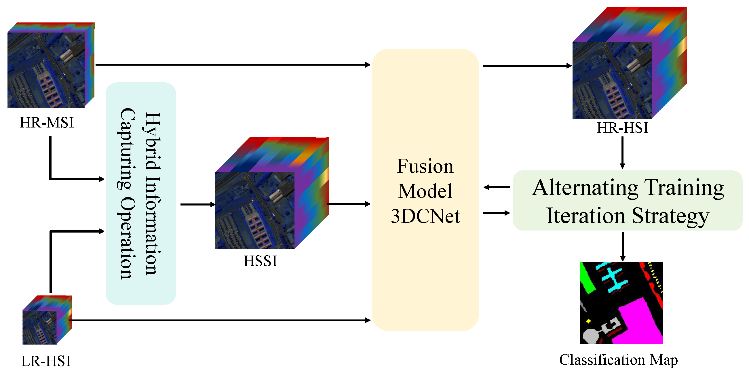
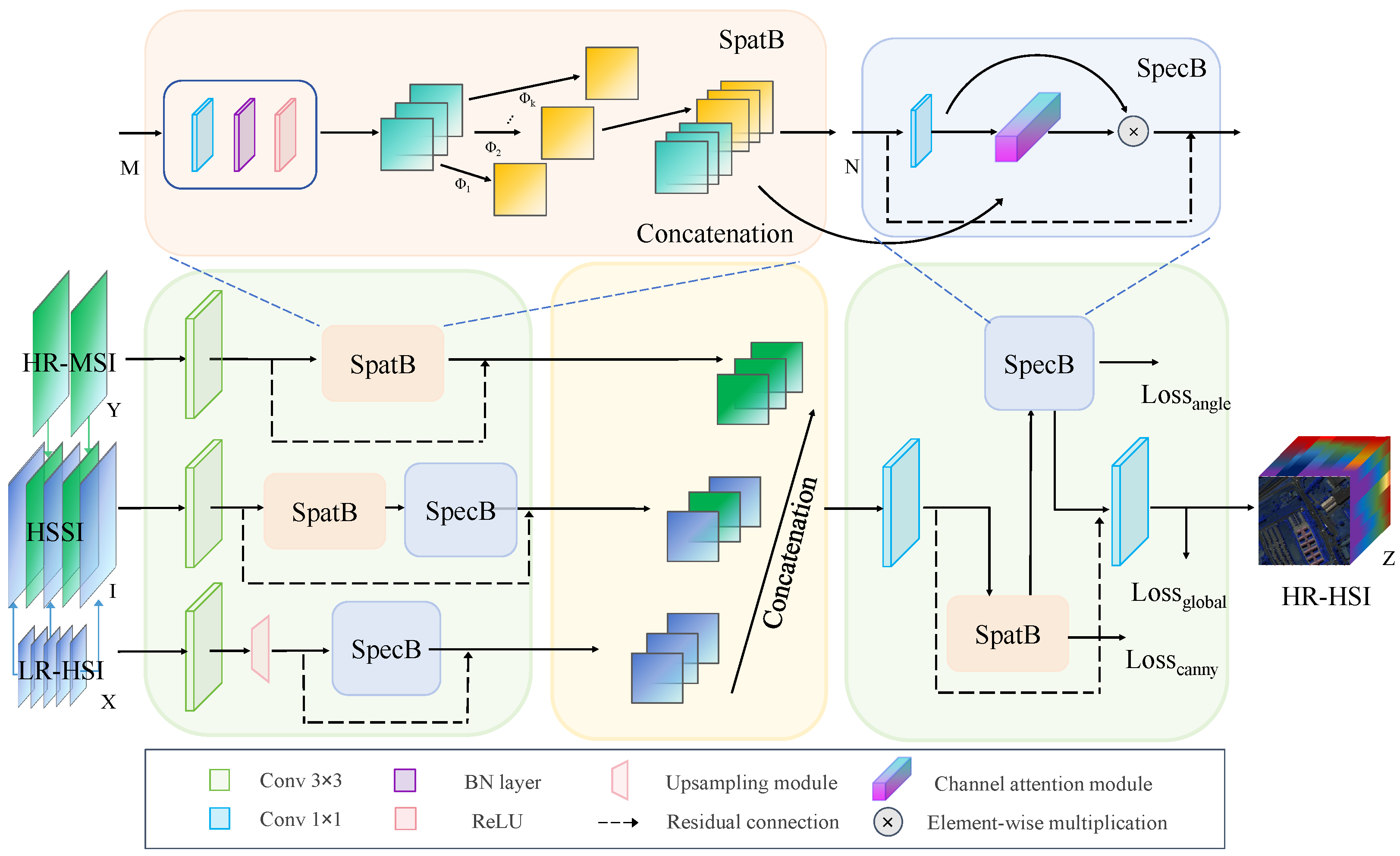
• A novel, efficient three-stream fusion network, 3DCNet, is proposed for high-precision LR-HSI and HR-MSI fusion. Three stream means that three branches distill the features in the LR-HSI, HR-MSI, and hybrid spatial–spectral image (HSSI), respectively.
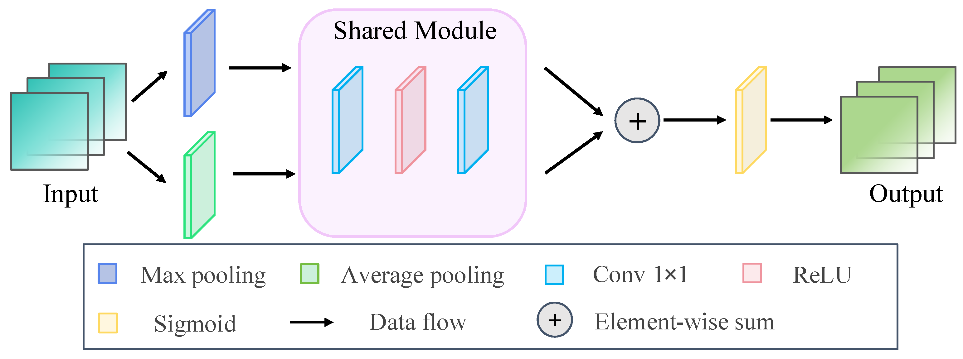
• For spatial and spectral feature extraction, low-cost linear transformation operations are utilized in spatial blocks (SpatBs) to effectively extract spatial information, while the channel attention mechanism in spectral blocks (SpecBs) is leveraged to capture global spectral information.
• In order to direct our 3DCNet to acquire precise feature representations, the loss function is segmented into three distinct parts: ${\mathcal{L}}_{global}$, ${\mathcal{L}}_{canny}$, and ${\mathcal{L}}_{angle}$. Beyond the global control of HR-HSI generation by ${\mathcal{L}}_{global}$, the Canny operator is employed to constrain the neural network, focusing it on the reconstruction of spatial texture details, while ${\mathcal{L}}_{angle}$ is utilized to control the fidelity of the generated HR-HSI by minimizing the variation in the spectral dimension.
• For downstream classification application, the alternating training iteration strategy (ATIS) is designed to iteratively train our fusion network alongside the classification network DBDA [18], with the aim of leveraging knowledge from each other, generating an HR-HSI that not only excels in visual and statistical performance but also minimizes the error in accuracy for the downstream high-level classification task.

The remainder of this article is organized as follows: Section 2 provides an overview of the related works on LR-HSI and HR-MSI fusion methods. In Section 3, 3DCNet and ATIS are proposed in detail. Section 4 designs and analyzes fusion experiments on seven datasets and classification experiments on four datasets, along with thorough ablation experiments. Conclusions are provided in Section 5.

2. Related Work

In this section, we first review the traditional methods and deep learning methods used in HSI and MSI fusion tasks. Second, we introduce some fusion methods leveraging knowledge from downstream high-level applications.

2.1. Traditional Fusion Methods

Prior to the emergence of deep learning, the traditional fusion methods were fundamentally structured around three principal categories.

(1) Matrix Factorization-based Methods: Matrix factorization-based fusion methods reinterpret the spatial dimensions of 3D HSIs alongside the spectral dimension, effectively flattening them into a two-dimensional matrix for processing. They decompose them into a spectral basis matrix and a coefficient matrix, and they consider the estimation of the spectral basis and coefficients as an optimization problem.

Kawakami et al. [4] employed sparse encoding algorithms to extract sparse coefficients from LR-HSIs, complemented by sparse dictionary learning methods to derive spectral dictionaries from HR-MSIs. Building upon this, Akhtar et al. [5] introduced a greedy algorithm for calculating sparse coefficients, incorporating the local similarity of the fused HSI into their calculations. Simoes et al. [6] expanded on this by considering both the spatial local similarity and the spectral characteristics of HSIs, employing a non-local sparse representation method to guide the optimization process. Dong et al. [7] further refined the approach by utilizing a sparse representation method with self-similarity constraints to guide the optimization.

Despite these advancements, matrix factorization-based methods have a critical limitation: they tend to overlook the intrinsic three-dimensional nature of HSI data. This oversight can result in a significant loss of information during the fusion process, highlighting the need for more sophisticated approaches that can preserve the rich spectral and spatial information inherent in HSIs.

(2) Tensor Decomposition-based Methods: Tensor decomposition-based methods take a direct approach to the fusion of LR-HSIs and HR-MSIs by treating HSI data as three-dimensional tensors, conceptualizing the fusion task as a tensor operation. Li et al. [8] introduced an innovative paradigm that leverages the Tucker decomposition model, coupled with Coupled Sparse Tensor Factorization (CSTF), for the fusion process. This approach decomposes the HR-HSI into a core tensor and three factor matrices, which are represented by dictionaries. The final estimation of the HR-HSI is derived from the estimation of these core tensors and dictionaries.

Kanatsoulis et al. [9] reformulated the factor matrix estimation into a least squares problem within the framework of canonical polynomial decomposition. In contrast, Dian et al. [10] employed singular value decomposition to learn spectral subspaces from LR-HSIs, estimated coefficients with the aid of low-tensor multi-rank priors, and utilized the clustering structure from HR-MSIs to group patches in the coefficients. The HR-HSI was then approximated using these spectral subspaces and coefficients.

Despite these methodological advancements, tensor decomposition-based methods are computationally intensive, demanding substantial computational resources, which can be a limiting factor in terms of algorithmic efficiency.

(3) Bayesian Estimation-based Methods: Bayesian estimation-based methods address the fusion of LR-HSIs and HR-MSIs from a statistical perspective, focusing on the prior distribution of the images. Hardie et al. [11] introduced a Maximum A Posteriori (MAP) estimator that employs a spatial variation statistical model derived from vector quantization to effectively harness local correlation information.

Zhang et al. [12] defined an innovative operator to articulate the spatial degradation inherent in HSI images. They employed a Bayesian framework with wavelet transform to describe and address the fusion problem by calculating this operator.

Akhtar et al. [13] took a probabilistic approach to infer the distribution and proportion of spectral information for different materials within HR-HSIs. Utilizing these distributions, they engaged in extensive research on the calculation of sparse encoding within HR-HSIs and proposed a Bayesian sparse encoding strategy. They further advanced the field by learning a Bayesian dictionary through the Beta process.

However, the probabilistic nature of these estimation methods inherently involves a degree of randomness, which may not always ensure optimal fusion outcomes.

2.2. Deep Learning-Based Fusion Methods

The development of deep learning has revolutionized the domain of image processing, with significant achievements made in recent years [19,20,21]. Its simplicity and effectiveness have also been demonstrated in the realm of HSI processing [22,23,24,25,26]. Deep learning approaches conceptualize the fusion of LR-HSIs and HR-MSIs as the establishment and refinement of fusion functions, which is tackled in a three-step process. Initially, a neural network is architected to serve as the fusion function, designed to exhaustively capture spatial and spectral image information. Following this, a loss function is carefully defined to guide the optimization process of the fusion function. The sequence of steps is ultimately concluded by employing a gradient descent algorithm to steer the loss function towards an optimal solution.

Masi et al. [27] employed a Convolutional Neural Network (CNN) with a stacked single-branch architecture to distill features from HSIs, marking one of the pioneering efforts directly applicable to the fusion challenge between HSIs and MSIs [28]. Palsson et al. [29] employed 3D-CNNs for image information extraction, incorporating PCA (Principal Component Analysis) priors to enhance the extraction process. Zhang et al. [14] introduced an innovative approach by integrating some spectral bands from HR-MSIs into LR-HSIs to create a composite image, subsequently leveraging a single-branch CNN to extract its features.

To fully leverage the complementary information in HSIs and MSIs, Yang et al. [15] crafted a dual-branch CNN that independently extracts spectral information from LR-HSIs and spatial information from HR-MSIs, merging these streams for a comprehensive fusion. Xu et al. [28] similarly designed a dual-branch network, progressively integrating extracted information from LR-HSIs and HR-MSIs across various scales. Yao et al. [30] introduced a cross-attention module to extract additional spatial information from HR-MSIs, which facilitates a more effective transmission of spatial–spectral information within the network architecture. Zhu et al. [31] proposed a new QIS strategy that combines the hierarchical structure of quadtrees with Implicit Neural Representations (INRs) and further enhances the fidelity of fused images by leveraging a Generative Adversarial Network (GAN) framework.

Neural networks have the advantages of modularity and efficiency, and fusion methods based on deep learning can lead to excellent fusion effects. However, the errors and redundancies introduced by them can reduce the effectiveness of downstream high-level visual applications.

2.3. Fusion Methods for Downstream Applications

The domain of image fusion, particularly in the context of visible and infrared images, has witnessed a surge of effective research on downstream high-level applications in recent years. Tang et al. [32] introduced a framework that concurrently trains models for visible and infrared image fusion and semantic segmentation of the fused output. This approach was later expanded by the same author [33], who transitioned from feature-level to image-level fusion, demonstrating that the latter could achieve superior performance in advanced visual tasks. However, although these works feed the performance of downstream applications back into the fusion process, they risk concentrating the focus towards those applications, potentially compromising the quality of fusion itself.

In the field of hyperspectral fusion, existing methods for fusing LR-HSIs and HR-MSIs have predominantly focused on visual quality and statistical metrics, with limited attention paid to their other roles in supporting downstream applications such as image classification [34] and object detection [35]. He et al. [17] introduced a novel strategy that aims to jointly optimize the super-resolution of HSIs and the downstream visual task of object detection in an effort to enhance both concurrently. However, this traditional method-based approach did not exploit the strengths of end-to-end trained neural networks.

To the best of our knowledge, there remains a lack of research in the hyperspectral and multispectral fusion domain that integrates low-level fusion knowledge and high-level task knowledge reciprocally within each other’s network training process. This highlights an opportunity for further exploration and innovation.

3. Methodology

In this section, the data preprocessing method is first introduced. Then, our three-stream fusion network for downstream classification application, 3DCNet, is proposed comprehensively, which is shown in Figure 2. Afterwards, the feature extraction blocks, SpatB and SpecB, are introduced in detail. Subsequently, we present the global fusion loss ${\mathcal{L}}_{global}$, spatial canny loss ${\mathcal{L}}_{canny}$, and spectral angle loss ${\mathcal{L}}_{angle}$. Ultimately, the alternating training iteration strategy (ATIS) is designed to enhance the efficacy of the predicted output for downstream classification tasks.

3.1. Hybrid Spatial–Spectral Image

In the proposed 3DCNet, the reference HR-HSI and the predicted HR-HSI are written as $\mathbf{R}\in {\mathbb{R}}^{H\times W\times C}$, $\mathbf{Z}\in {\mathbb{R}}^{H\times W\times C}$, respectively, where H, W, and C represent the height, width, and number of channels or bands, respectively. The input LR-HSI and HR-MSI are denoted as $\mathbf{X}\in {\mathbb{R}}^{h\times w\times C}\left(h\ll H,w\ll W\right)$ and $\mathbf{Y}\in {\mathbb{R}}^{H\times W\times c}\left(c\ll C\right)$. First, the LR-HSI is upsampled spatially to match the spatial resolution of the HR-MSI.

$$X_{up}=Bilinear\left(\mathbf{X},r\right)$$

(1)

where $X_{up}$ represents the upsampled LR-HSI, and r is the ratio. Bilinear means the bilinear interpolation operation.

To fully extract the information shared between the HR-MSI and LR-HSI, $\mathbf{Y}$ is inserted at equal intervals along the spectral dimension into $X_{up}$, resulting in hybrid spatial–spectral image (HSSI), written as $\mathbf{I}$. The insertion position can be formulated as

$$p_i=⌊{\displaystyle \frac{C·i}{c+1}}⌋+1,i=1,2,\cdots ,c$$

(2)

where $p_i$ denotes the insertion position of the i-th multispectral band. Then, the HSSI is computed as

$$\mathbf{I}\left(k\right)=\left\{\begin{array}{cc}{X}_{up}\left(k\right),\hfill & \mathrm{if}k\notin \{p_1,p_2,\cdots ,p_c\}\hfill \\ \mathbf{Y}\left(k\right),\hfill & \mathrm{if}k=p_i,i=1,2,\cdots ,c\hfill \end{array}\right.$$

(3)

where k is the k-th spectral band. By this approach, the resulting $\mathbf{I}$ integrates the spectral information from the LR-HSI with the spatial details from the HR-MSI.

3.2. Three-Stream HSI and MSI Fusion Network

In Figure 2, the overall architecture of our proposed 3DCNet is presented. It mainly consists of three branch networks and a global network. From top to bottom, the three branch networks extract the spatial features of $\mathbf{Y}$, the spatial and spectral features of $\mathbf{I}$, and the spectral features of $\mathbf{X}$, respectively. Then, the features are combined into fused feature maps through the concatenation operation. The features in the fused feature maps are comprehensively extracted by the spatial and spectral blocks of the global network, with the final output being generated as $\mathbf{Z}$.

(1) The Branch Network: Specifically, in order to extract the shallow feature maps of $\mathbf{Y}$, a simple 3 × 3 convolutional layer is used.

$$Y_{conv}=Conv(\mathbf{Y},3)$$

(4)

where Conv represents the convolutional operation, and 3 represents the kernel size. Then, the shallow feature map is passed to the spatial block, with a residual connection. We have

$$Y_{out}={Spat}_{res}\left(Y_{conv}\right)$$

(5)

where Spat refers to the spatial block, and $res$ refers to the residual connection. The residual connection is used to alleviate the vanishing gradient problem, which allows the network to be built deeper, enabling the extraction of deep-level features. Similarly, the output of the HSI branch $X_{out}$ can be formulated as

$$\left\{\begin{array}{c}{X}_{conv}=Conv(\mathbf{X},3)\hfill \\ X_{up}=Bilinear(X_{conv},r)\hfill \\ X_{out}={Spec}_{res}\left(X_{up}\right)\hfill \end{array}\right.$$

(6)

where Spec represents the data flow passing through the spectal block.

The intermediate branch of the network converts $\mathbf{I}$, which integrates spatial information and spectral information, into feature maps and extracts their deep-level features. The formula can be written as

$$\left\{\begin{array}{c}{I}_{conv}=Conv(\mathbf{I},3)\hfill \\ I_{out}={Spat-spec}_{res}\left(I_{conv}\right)\hfill \end{array}\right.$$

(7)

where Spat−spec denotes the module that connects the spatial block and the spectral block in series in order to extract spatial and spectral messages.

Before feeding the deep features into the following global network, we use the concatenation operation to gather feature maps,

$$Z_{in}=Conc(Y_{out},I_{out},X_{out})$$

(8)

where $Z_{in}$ represents the concatenated feature maps, and Conc denotes the concatenation operation. It should be noted that all convolutional layers and the spatial and spectral blocks used in the branch network are designed to maintain the same H, W, and C of the data flow for convenience.

(2) The Global Network: After obtaining the concatenated feature maps $Z_{in}$, the global network is utilized to further extract features. Here, the convolution layer using a 1 × 1 kernel size instead of a 3 × 3 kernel size is utilized to extract features. One reason for this is that $Z_{in}$ has too many channels, and a 1 × 1 kernel size, in comparison, can reduce the number of parameters. The other reason is that the 1 × 1 convolutional operation is used to change the channels of feature maps into the same as $\mathbf{R}$. This can be written as

$$Z_{conv}=Conv(Z_{in},1)$$

(9)

Then, the feature maps are sent into the spatial block and the spectral block sequentially. A point to be aware of is that data flow in the global network after the first Conv 1 × 1 maintains the same number of channels as $\mathbf{X}$, $\mathbf{Y}$, $\mathbf{Z}$, and $\mathbf{R}$. This approach is taken for the convenience of using the loss function, which is introduced later. The data flow can be fomulated as

$$Z_{out}={Spat-spec}_{res}\left(Z_{conv}\right)$$

(10)

Eventually, the feature maps are fed into the last 1 × 1 convolutional layer to generate the final output,

$$\mathbf{Z}=Conv(Z_{out},1)$$

(11)

where $\mathbf{Z}$ is the predicted HR-HSI.

3.3. SpatB and SpecB

Previous fusion research has made strides with dual-branch networks capable of extracting information from both LR-HSIs and HR-MSIs [28,36]. However, these works did not introduce specialized modules tailored to the distinct characteristics of spatial and spectral information. Drawing inspiration from Ghostnet [37], we design our spatial block (SpatB) to exhaustively capture spatial details. Similarly, we leverage the attention mechanism from CBAM [38] to conceive the spectral block (SpecB), ensuring the comprehensive extraction of spectral information across the global scale.

(1) SpatB: The upper left corner of Figure 2 shows the entire architecture of the spatial block (SpatB). In the SpatB, we denote the input as $M_{in}$ and the output as $M_{out}$. Firstly, $M_{in}$ is fed into the Conv 1 × 1 layer, the batch normalization (BN) layer, and the rectified linear unit (ReLU) activation function sequentially, which can be formulated as

$$\left\{\begin{array}{c}{M}_{conv}=Conv(M_{in},1)\hfill \\ M_{bn}=BN\left(M_{conv}\right)\hfill \\ M_{relu}=ReLU\left(M_{bn}\right)\hfill \end{array}\right.$$

(12)

where BN denotes the batch normalization operation, which normalizes each mini-batch of data. This can reduce the risk of overfitting and help accelerate the training speed of the neural network. ReLU refers to the rectified linear unit activation function, which introduces nonlinearity into the neural network and enables it to model complex functional mappings.

Subsequently, the feature maps derived from $M_{relu}$ are separated individually along the channel dimension. From these separated feature maps, ghost feature maps are generated through a series of low-cost linear transformation operations denoted as ${\Phi }_k$. It should be noted that these operations are applied individually to each channel through convolution, thereby significantly reducing computational expenses. These ghost feature maps are then concatenated with the feature maps of $M_{relu}$, and the concatenated output is collectively delivered from the SpatB, being the final output $M_{out}$. These can be detailed as

$$\left\{\begin{array}{c}{M}_{\varphi }^k={\Phi }_k\left(M_{relu}^k\right),k\in \{1,...,K\}\hfill \\ M_{out}=Conc(M_{relu},M_{\varphi })\hfill \end{array}\right.$$

(13)

where k represents the kth channel within the feature maps, while K signifies the total channels of the feature maps. The notation ${\Phi }_k$ refers to different low-cost linear transformation operations, which can be implemented by different Conv 1 × 1 operations mathematically.

(2) SpecB: In contrast to the SpatB, the SpecB concentrates on the spectral dimension. The upper right corner of Figure 2 shows the SpecB, which employs Conv 1 × 1 to extract shallow-level features from $N_{in}$, generating $N_{conv}$. Subsequently, it utilizes an attention mechanism along the channel dimension, producing $N_{atte}$.

The adjacent spectral bands in the HSI exhibit strong correlations, which is applied to HSI unmixing and HSI super-resolution tasks [39,40]. This rich spectral information is a distinctive attribute that sets HSIs apart from conventional RGB images. To fully leverage the abundant spectral information of the HSI, each channel in the ensuing feature maps can be regarded as a linear superposition of all spectral channels in the preceding feature maps [41]. The coefficients of this linear superposition correspond to the weights derived from the the Conv 1 × 1 operation mathematically, which is utilized in the SpecB. The formulation is as follows:

$$N_{conv}=Conv(N_{in},1)$$

(14)

The channel-wise attention mechanism is inspired by CBAM [38], which adaptively modulates the feature scale in each channel by considering their cross-spectral interdependencies. The detailed channel-wise attention mechanism is shown in Figure 3. Specifically, max pooling and average pooling operations are applied to downsample the feature maps across spatial dimensions, thereby preserving the intrinsic channel characteristics. The max pooling operation is conducive to identifying prominent features, while average pooling ensures the inclusion of global features. These pooled features are then processed through a shared module, which is designed to refine feature representation. Subsequently, the outputs from the shared module are added together through an element-wise summation, and the resultant feature maps are then passed through a Sigmoid activation function to derive the final channel attention weights. The formulation process can be written as

$$\left\{\begin{array}{c}{N}_{maxp}=Pool(N_{conv},max)\hfill \\ N_{avep}=Pool(N_{conv},ave)\hfill \\ N_{mlp}=Shared\left(N_{maxp}\right)+Shared\left(N_{avep}\right)\hfill \\ N_{atte}=Sigmoid\left(N_{mlp}\right)\hfill \end{array}\right.$$

(15)

where Pool denotes the pooling operation, and $max$ and $ave$ represent the max pooling and average pooling operations. Shared refers to the shared module, which sequentially consists of a Conv 1 × 1 layer, a ReLU activation function, and another Conv 1 × 1 layer. Sigmoid refers to the Sigmoid activation function.

Back to the SpecB, $N_{atte}$ then serves as the coefficient to automatically adjust $N_{conv}$. Following this, $N_{atte}$ and $N_{conv}$ go through element-wise multiplication at their corresponding positions, resulting in feature maps that are scaled through the attention mechanism. Finally, the output of the SpecB, $N_{out}$, is obtained via a residual connection. The details are written as

$$\left\{\begin{array}{c}{N}_{mult}=N_{atte}\ast N_{conv}\hfill \\ N_{out}=N_{in}+N_{mult}\hfill \end{array}\right.$$

(16)

where ∗ represents the element-wise multiplication. $N_{out}$ denotes the result of applying the residual connection operation.

3.4. Loss Function

The inherent black-box nature of neural networks results in an uncontrollable feature map learning process. Therefore, a carefully crafted loss function for HSI data is essential to better guide the parameter updating process. Empirical evidence from various studies indicates that the $L_1$ norm loss is effective in penalizing minor errors, thereby reducing the blurring effects associated with image smoothing. However, the $L_1$ norm loss is sensitive to parameter initialization and necessitates careful hyperparameter tuning. In contrast, the $L_2$ norm loss exhibits robustness against the initialization of parameters, yielding more stable solutions. Its differentiability across the entire domain further contributes to the stability of the optimization process. By carefully designing the loss function for both spatial and spectral features, it becomes feasible to compensate for the image blurring problems that may arise from the $L_2$ norm loss. Specifically, the global fusion loss is formulated as

$${\mathcal{L}}_{global}={\displaystyle \frac{1}{HWC}}\sum _{h=1}^H\sum _{w=1}^W\sum _{c=1}^C{\parallel \mathbf{R}(h,w,c)-\mathbf{Z}(h,w,c)\parallel }_2$$

(17)

where $\mathbf{R}(h,w,c)$ and $\mathbf{Z}(h,w,c)$ represent the element in the reference HR-HSI and the predicted HR-HSI, respectively.

However, the aforementioned loss functions target the overall quality of the generated HR-HSI. Despite the low spatial resolution of HSIs, their spatial textural features play an important role in tasks such as classification and target detection. Therefore, our 3DCNet incorporates a spatial loss function.

Image edges, referring to locally discontinuous image features, are critical for capturing rich texture information. To effectively extract these edge features, we employ the Canny operator [42], a widely recognized and utilized algorithm for edge detection in the field of image processing. The Canny operator offers the dual advantages of noise suppression and the ability to detect fine-grained edges. The implementation specifics are as follows:

$${\mathcal{L}}_{canny}=MSE(Canny\left({\mathbf{Z}}_{spat}\right),Canny(\mathbf{R}\left)\right)$$

(18)

where MSE denotes the mean square error, and Canny denotes the Canny operator. It is crucial to note that our spatial loss function, ${\mathcal{L}}_{canny}$, compares the output from the SpatB, $Z_{spat}$, against the reference $\mathbf{R}$. This comparison is instrumental in guiding the network’s data flow process.

Compared with RGB images, a notable feature of HSIs is that hundreds of spectral bands contain rich spectral information. This distinctive feature demands that our loss function precisely quantifies the spectral differences between the predicted HR-HSI and the reference HR-HSI. Given that HSIs are treated as 3D tensors in computation, the angular deviation between these tensors serves as a robust metric for assessing the similarity between the predicted and reference images. Inspired by the methodology presented in [28], we utilize ${\mathcal{L}}_{angle}$ to ensure the spectral fidelity, which is designed as follows:

$$\left\{\begin{array}{c}Angle={\displaystyle \frac{1}{HW}}\sum _{h=1}^H\sum _{w=1}^{W}arcos{\displaystyle \frac{{\mathbf{R}}_c^{\top }·{\mathbf{Z}}_c}{{∥{\mathbf{R}}_c∥}_2{∥{\mathbf{Z}}_c∥}_2}}\hfill \\ \\ {\mathcal{L}}_{angle}=MSE(Angle\left({\mathbf{Z}}_{out}\right),Angle\left(\mathbf{R}\right))\hfill \end{array}\right.$$

(19)

where arcos represents the arccosine operation, and ⊤ refers to the transpose of the tensor. ${\mathbf{R}}_c$ and ${\mathbf{Z}}_c$ represent the vectors of the same pixel along the cth channel in $\mathbf{R}$ and $\mathbf{Z}$, respectively.

In summary, the total loss function of our proposed 3DCNet consists of the above three parts and is written as

$${\mathcal{L}}_{total}={\lambda }_1{\mathcal{L}}_{global}+{\lambda }_2{\mathcal{L}}_{canny}+{\lambda }_3{\mathcal{L}}_{angle}$$

(20)

At last, it is worth pointing out that plenty of experiments show that the coefficients of these three loss functions should be set to ${\lambda }_1=10$, ${\lambda }_2={\lambda }_3=1$.

3.5. Alternating Training Iteration Strategy

In the domain of HSI processing, the HR-HSI fusion models and the downstream HSI classification models are typically trained in isolation. This method, although effective for individual model optimization, can result in discrepancies between the reference data and the fused HR-HSI, potentially impairing the efficacy of the downstream classification task.

Tang et al. [32] introduced a joint adaptive training strategy for the fusion and segmentation tasks of infrared and visible light images. However, this strategy primarily integrates the segmentation network’s performance into the fusion network, potentially overemphasizing the downstream network’s training. This could disrupt the balance between low-level and high-level visual tasks.

We refine this approach in the training fusion and downstream classification networks. Specifically, the fusion model and the classification model are trained repeatedly over multiple cycles. During each training cycle of the fusion network, the classification network’s inference loss ${\mathcal{L}}_{ce}$ from the previous round is reintegrated into the fusion loss function. Reciprocally, during each iteration of the classification network’s training, the fusion network’s inference loss ${\mathcal{L}}_{total}$ from the last training session is reintegrated into the classification loss function. It is worth noting that our classification network is the DBDA network from [18], which has demonstrated superior performance when trained on reference images. The details of our iterative strategy is shown in Algorithm 1.

In Algorithm 1, ${\mathcal{L}}_{class}$ represents the classification loss function, and ${\mathcal{L}}_{ce}$ refers to the cross-entropy loss, which is defined as

$${\mathcal{L}}_{ce}=\sum _{m=1}^L{y}_m(log(\sum _{n=1}^L{e}^{\widehat{y_n}})-\widehat{y_m})$$

(21)

where L represents the total count of labeled pixels, and $y_m$ and $y_n$ denote the categories of the mth and nth pixels, respectively. The coefficients of these loss functions are set to ${\lambda }_4=10$ and ${\lambda }_5=0.1$.

Algorithm 1 Alternating Training Iteration Strategy

1: Input: LR-HSI $\mathbf{Y}$ and HR-MSI $\mathbf{X}$   2: Output: Fused HR-HSI $\mathbf{Z}$   3: Initial: Loop variable $n=0$   4: while $n\le N$ do   5:    for p iterations do   6:       Randomly select the LR-HSI region ${\mathbf{Y}}^i$ and               the corresponding HR-MSI region ${\mathbf{X}}^i$;   7:       Calculate the fusion loss:               ${\mathcal{L}}_{fusion}^i={\mathcal{L}}_{total}^i+{\lambda }_4·n·{\mathcal{L}}_{ce}^i$;   8:       Update parameters of the fusion network $N_{\mathcal{F}}$               by Adam optimizer: ${\nabla }_{N_{\mathcal{F}}}\left({\mathcal{L}}_{fusion}^i\right)$;   9:    end for 10:    Generate fused HR-HSI $\mathbf{Z}$ from $\mathbf{Y}$ and $\mathbf{X}$ using             the training set; 11:    Select $t\%$ labeled data from the fused HR-HSI             as training data $\mathbf{T}$; 12:    for q epochs do 13:       Select batched training samples ${\mathbf{T}}^i$; 14:       Calculate the classification loss:               ${\mathcal{L}}_{class}^i={\mathcal{L}}_{ce}^i+{\lambda }_5·n·{\mathcal{L}}_{total}^i$; 15:       Update parameters of the classification network               $N_{\mathcal{C}}$ by another Adam optimizer: ${\nabla }_{N_{\mathcal{C}}}\left({\mathcal{L}}_{class}^i\right)$; 16:    end for 17:    $n=n+1$; 18: end while

4. Experiments

This section presents a series of fusion experiments conducted on seven datasets, aimed at proving the generalization ability of our proposed 3DCNet. Downstream classification experiments are performed on the first four of these datasets to prove the effectiveness of our ATIS. The structure of this section is as follows: First, the experimental datasets and evaluation metrics are introduced. Following this, detailed experimental settings and a comparative analysis with nine cutting-edge methods are provided. Then, a series of ablation studies prove the indispensability of each model component and the validity of the ATIS. Finally, the section ends with efficiency experiments and a hyperparameter sensitivity analysis.

4.1. Dataset

In this article, seven datasets are used to validate the generalization performance of our 3DCNet, namely, the Pavia University, Pavia Center, Indian Pines, Botswana, Washington DC Mall, Urban, and CAVE datasets. The first four datasets are utilized to assess the ATIS’s efficacy, as their labeled samples are relatively dispersed, which helps to crop the testing data.

(1) Pavia University: The Pavia University dataset was captured by ROSIS sensors over Pavia University in Italy. After removing samples without any information, the dataset consists of 610 × 340 pixels and 103 spectral bands, with wavelengths ranging from 0.43 to 0.86 μm at a spatial resolution of 1.3 m. This dataset contains nine categories, such as asphalt, trees, and bare soil.

(2) Pavia Center: The Pavia Center dataset was captured by ROSIS sensors over Pavia Center in Italy. After removing samples that do not contain any information, the dataset consists of 1096 × 1096 pixels and 102 spectral bands, with wavelengths ranging from 0.43 to 0.86 μm at a spatial resolution of 1.3 m. This dataset contains nine categories, such as water, trees, and bare soil.

(3) Indian Pines: The Indian Pines dataset was collected by AVIRIS sensors over the Indian Pines test site in northwestern Indiana. After removing bands covering the water absorption area, the dataset consists of 145 × 145 pixels and 200 spectral bands, with wavelengths ranging from 0.4 to 2.5 μm. The available ground truth is divided into 16 categories, such as alfalfa, soybean mint, and woods.

(4) Botswana: The Botswana dataset contains a sequence of data captured by the Hyperion sensor on the EO-1 satellite over Okavango Delta, Botswana. After removing bands that cover the water absorption characteristics, the dataset consists of 1476 × 256 pixels and 145 bands, with spectral wavelengths ranging from 0.4 to 2.5 μm at a spatial resolution of 30 m. This dataset contains 14 determined categories, representing water, reeds, island interval, etc.

(5) Washington DC Mall: The Washington DC Mall dataset contains aerial hyperspectral images obtained by a Hydice sensor over the Washington shopping center. This dataset consists of 1280 × 307 pixels and 191 bands, with spectral bands ranging from 0.4 to 2.5 μm.

(6) Urban: The Urban dataset was collected in Copperas Cove, TX, USA. After removing the dense water vapor and atmospheric bands, the dataset consists of 307 × 307 pixels and 162 bands at a spatial resolution of 2 m, with wavelengths ranging from 0.4 to 2.5 μm.

(7) CAVE: The CAVE dataset consists of 32 hyperspectral images acquired indoors, each measuring 512 by 512 pixels, with 31 spectral bands spanning wavelengths from 0.4 μm to 0.7 μm at 10 nm intervals.

4.2. Evaluation Metrics

Five widely used fusion metrics are used to evaluate the performance of our 3DCNet and other comparison methods, and three commonly used classification metrics are used to evaluate the performance of downstream classification performance. The following five metrics represent fusion effects from different aspects.

(1) Root Mean Square Error: The RMSE measures the distance between the reference image and the predicted image but is sensitive to outliers in the data.

$$RMSE=\sqrt{{\displaystyle \frac{{\sum }_{c=1}^C{\sum }_{h=1}^H{\sum }_{w=1}^W{(\mathbf{R}-\mathbf{Z})}^2}{HWC}}}$$

(22)

where $\mathbf{R}$ represents the reference HR-HSI, and $\mathbf{Z}$ refers to the predicted HR-HSI. C, H, and W correspond to the number of channels or bands, height, and width of the HSI, respectively. The smaller the RMSE, the better the performance.

(2) Peak Signal to Noise Ratio: The PSNR is one of the most commonly used indicators to measure image quality:

$$PSNR=10·{log}_{10}\left({\displaystyle \frac{max{\left({\mathbf{R}}_c\right)}^2}{\frac{1}{HW}{∥{\mathbf{R}}_c-{\mathbf{Z}}_c∥}_2^2}}\right)$$

(23)

where ${\mathbf{R}}_c$ and ${\mathbf{Z}}_c$ represent the cth channel of the reference image and the predicted image, respectively. ${∥·∥}_2$ means the second norm. After adding up the PSNRs of all channels, we obtain the PSNR metric of the whole image. The larger the PSNR, the better the performance.

(3) Relative Dimensionless Global Error in Synthesis: ERGAS is an indicator used to evaluate the quality of remote sensing images [43]; it considers the mean square error and brightness information of the image to provide a comprehensive evaluation of the performance of the image. The definition formula is as follows:

$$ERGAS={\displaystyle \frac{100}{r}}\sqrt{{\displaystyle \frac{1}{C}}\sum _{c=1}^C{\displaystyle \frac{{∥{\mathbf{R}}_c-{\mathbf{Z}}_c∥}_2^2}{{\mu }^2\left({\mathbf{R}}_c\right)}}}$$

(24)

where r refers to the spatial downsampling ratio when we obtain the LR-HSI. $\mu \left({\mathbf{R}}_c\right)$ represents the mean value of the cth channel of the reference image. The lower the ERGAS value, the higher the image quality.

(4) Spectral Angle Mapper: The SAM is a spectral angle mapping that treats the spectrum of each pixel in an image as a high-dimensional vector [44]. The similarity between spectra is measured by calculating the angle between the two vectors. The SAM is defined as

$$SAM={cos}^{-1}\left({\displaystyle \frac{{\sum }_{c=1}^C{\mathbf{r}}_c{\mathbf{z}}_c}{\sqrt{{\sum }_{c=1}^C{\mathbf{r}}_c^2}\sqrt{{\sum }_{c=1}^C{\mathbf{z}}_c^2}}}\right)$$

(25)

where ${\mathbf{r}}_c$ and ${\mathbf{z}}_c$ refer to the spectral vectors of the reference and predicted HR-HSIs. The smaller the SAM, the more similar the two spectra.

(5) Structural Similarity Index Measure: The SSIM is an indicator used to measure the degree of similarity between two digital images [45]. Structural similarity aligns more closely with the human visual perception of image quality, providing a metric that better reflects the discernment of human eyes. The SSIM is formulated as

$$SSIM={\left[l(\mathbf{R},\mathbf{Z})\right]}^{\alpha }·{\left[c(\mathbf{R},\mathbf{Z})\right]}^{\beta }·{\left[s(\mathbf{R},\mathbf{Z})\right]}^{\gamma }$$

(26)

$$l(\mathbf{R},\mathbf{Z})={\displaystyle \frac{2{\mu }_{\mathbf{R}}{\mu }_{\mathbf{Z}}+C_1}{{\mu }_{\mathbf{R}}^2+{\mu }_{\mathbf{Z}}^2+C_1}}$$

(27)

$$c(\mathbf{R},\mathbf{Z})={\displaystyle \frac{2{\sigma }_{\mathbf{R}}{\sigma }_{\mathbf{Z}}+C_2}{{\sigma }_{\mathbf{R}}^2+{\sigma }_{\mathbf{Z}}^2+C_2}}$$

(28)

$$s(\mathbf{R},\mathbf{Z})={\displaystyle \frac{{\sigma }_{\mathbf{R}\mathbf{Z}}+C_3}{{\sigma }_{\mathbf{R}}{\sigma }_{\mathbf{Z}}+C_3}}$$

(29)

where l, c, and s represent a comparison of the brightness, contrast, and structure between the reference image and the predicted image, respectively. $\alpha ,\beta ,\gamma$ are weighting coefficients, typically set to 1. ${\mu }_{\mathbf{R}}$ and ${\mu }_{\mathbf{Z}}$ denote the average value of $\mathbf{R}$ and $\mathbf{Z}$, while ${\sigma }_{\mathbf{R}}$ and ${\sigma }_{\mathbf{Z}}$ denote the standard deviation. ${\sigma }_{\mathbf{R}\mathbf{Z}}$ denotes the covariance of $\mathbf{R}$ and $\mathbf{Z}$. The higher the SSIM, the better the performance.

In addition, the overall accuracy (OA) and average accuracy (AA) are used to evaluate the quality of classification performance. The Kappa coefficient (KAPPA) reflects the consistency between the ground truth and the classification results. The closer all three metrics to 1, the better.

4.3. Implementation Details

(1) Data Preprocessing: Due to the data scarcity of the remote sensing dataset, we select 128 × 128 pixels from the original dataset as the testing data, and we randomly crop 128 × 128 pixels from other regions in each iteration as the training data. During the training phase, we fill the testing area with 0 to ensure that the model does not use any testing data. In order to verify the effectiveness of our ATIS, we especially select regions containing more samples with different categories as the testing data. The specific regions to be cropped in each dataset are shown in

Table 1. Testing data region.

Dataset	Pixel Size	Left Top Position
Pavia University	$128\times 128$	$(211,106)$
Pavia Center	$128\times 128$	$(241,417)$
Indian Pines	$64\times 64$	$(1,1)$
Botswana	$128\times 128$	$(562,76)$
Washington DC Mall	$128\times 128$	$(576,89)$
Urban	$128\times 128$	$(89,89)$

. In particular, the Indian Pines dataset only has 145 × 145 pixels in total, so we replace the size of the training and testing sets with 64 × 64. In addition, the LR-HSI is obtained by the 5 × 5 Gaussian kernel blurring operation with a standard deviation of 2, and then it is downsampled with a ratio of 4, while the HR-MSI is simulated by selecting five bands located in the HR-HSI at equal intervals. All the above operations are proven effective in SSRNet [14]. For the CAVE dataset, we select 22 out of 32 pictures for training, while the remaining 10 are employed for testing purposes. We perform random translations, rotations, and shears on the training set of the CAVE dataset, expanding the number of images by a factor of 14.

(2) Training Details: When obtaining image edges, the Gaussian kernel size used in the Canny operator is 3 × 3 with a standard deviation of 1, while the low threshold is set to $0.15$, and the high threshold is set to $0.30$. Four traditional methods, namely, CNMF [39], LTTR [46], NSSR [7], and CTDF [47], as well as eight deep learning methods, namely, TFNet [36], ResTFNet [36], SSF [48], ConSSF [48], MSDCNN [49], SSRNet [14], MSST [16], and DCFormer [50], are used as a comparison.

For traditional methods, everything else remains consistent with the original papers, except for data preprocessing. To avoid the influence of different dimensions and numerical ranges, as well as to accelerate the convergence speed of the algorithms, we standardize all data to a range of 0–255 by using the Min–Max Scaler. For deep learning methods, the same experimental setup as the original papers [14] is adopted, specifically using Adam as the optimizer, with a learning rate of 1 × 10⁻⁴. We mask the test region of the dataset, designating the remaining area as the training region. From the training region, we randomly sample 10,000 images to form the training set, with a batch size of 32. It should be noted that we are unable to implement MSDCNN using the Caffe framework, but Pytorch is used as an alternative. Additionally, the original SGD optimizer in the MSDCNN model is replaced with the more effective Adam optimizer.

Our model uses Adam as the optimizer with an initial learning rate of ${10}^{-3}$. The learning rate is adjusted using the exponential decay strategy, and the decay coefficient is set to $0.9995$, preventing network parameter oscillations in the later training stages.

As for the alternating training iteration strategy (ATIS), we set the best iteration count N to 4. When training the classification model, we fix the random seed to select the same training samples in each iteration, and the data preprocessing method is the same as that used by the fusion model. The batch size for the training samples of the classification model is set to 16, and the training epoch is set to 120, with all other parameters being consistent with the original settings in DBDA [18]. It should be noted that, we experiment with various sampling ratios for the training set of the DBDA network. An excessive number of samples can lead to model overfitting, while an insufficient number results in underfitting. Finally, for our task, the optimal training set sampling ratios are adopted as follows: Pavia University 1%, Pavia Center 0.5%, Indian Pines 5%, and Botswana 3%.

All deep learning methods are trained and tested in PyTorch 2.2.0 and Python 3.11 on an Intel Xeon Gold 6326 CPU (Intel Corporation, Santa Clara, CA, USA) and an NVIDIA GeForce RTX 4090 (NVIDIA Corporation, Santa Clara, CA, USA).

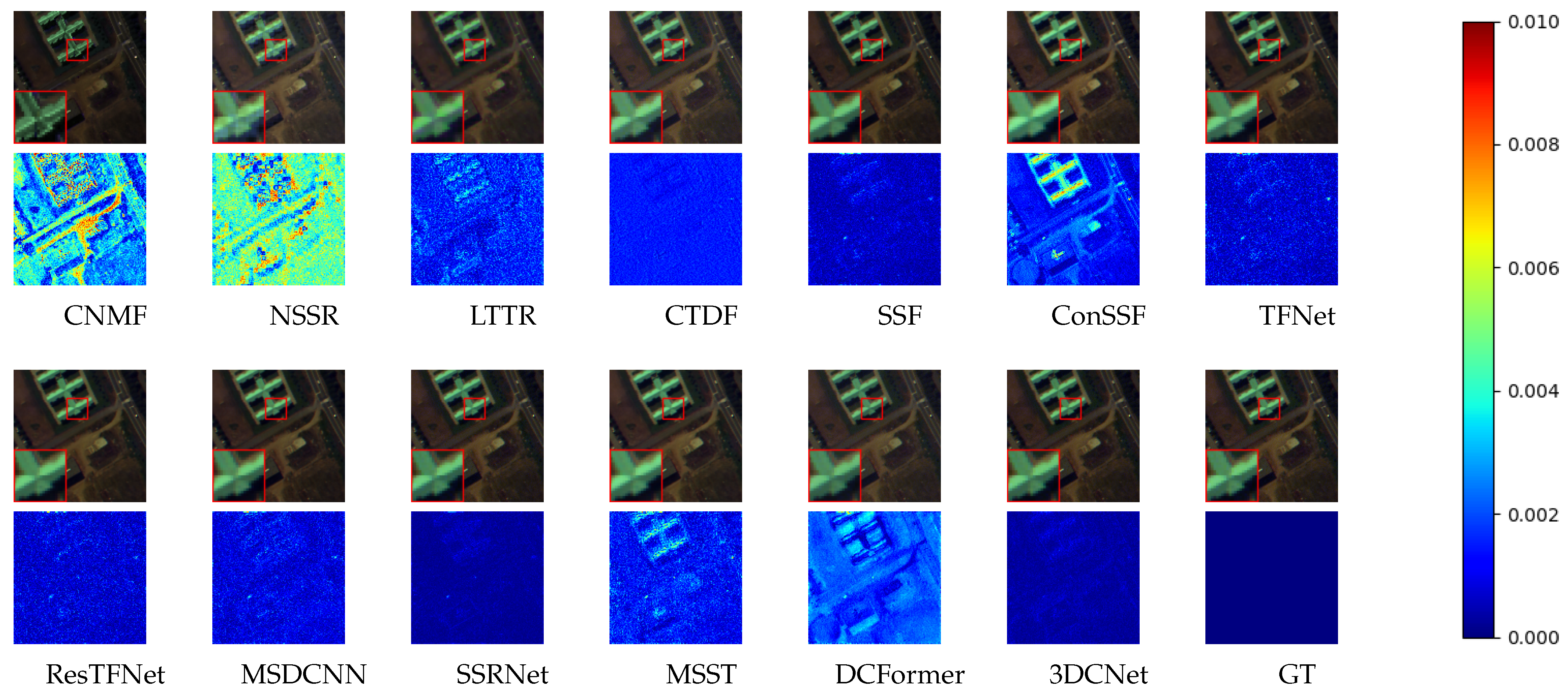
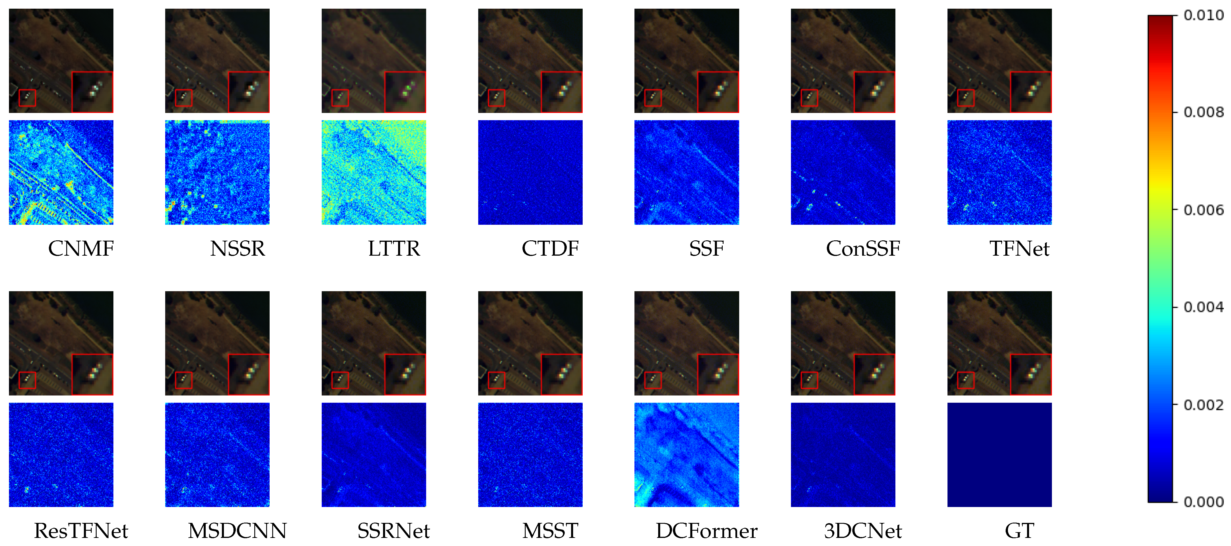
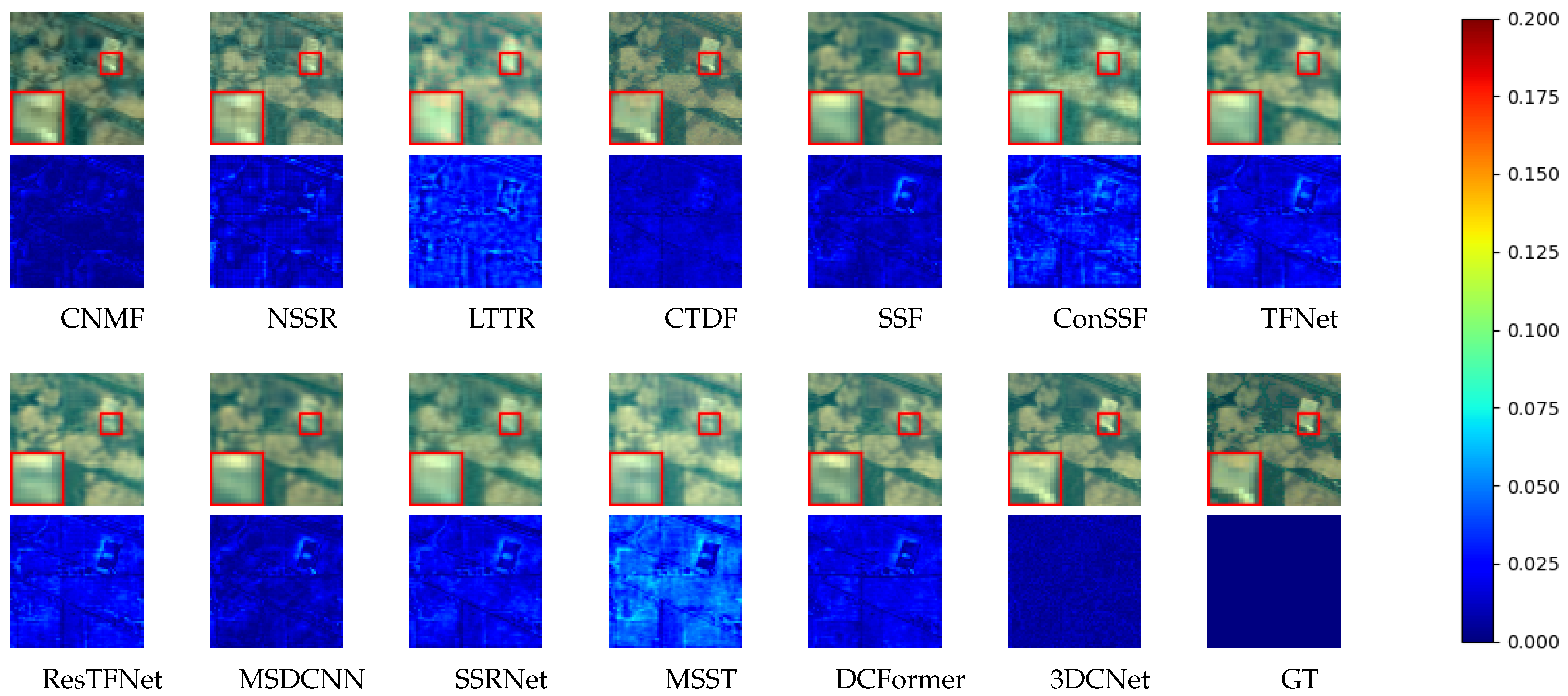
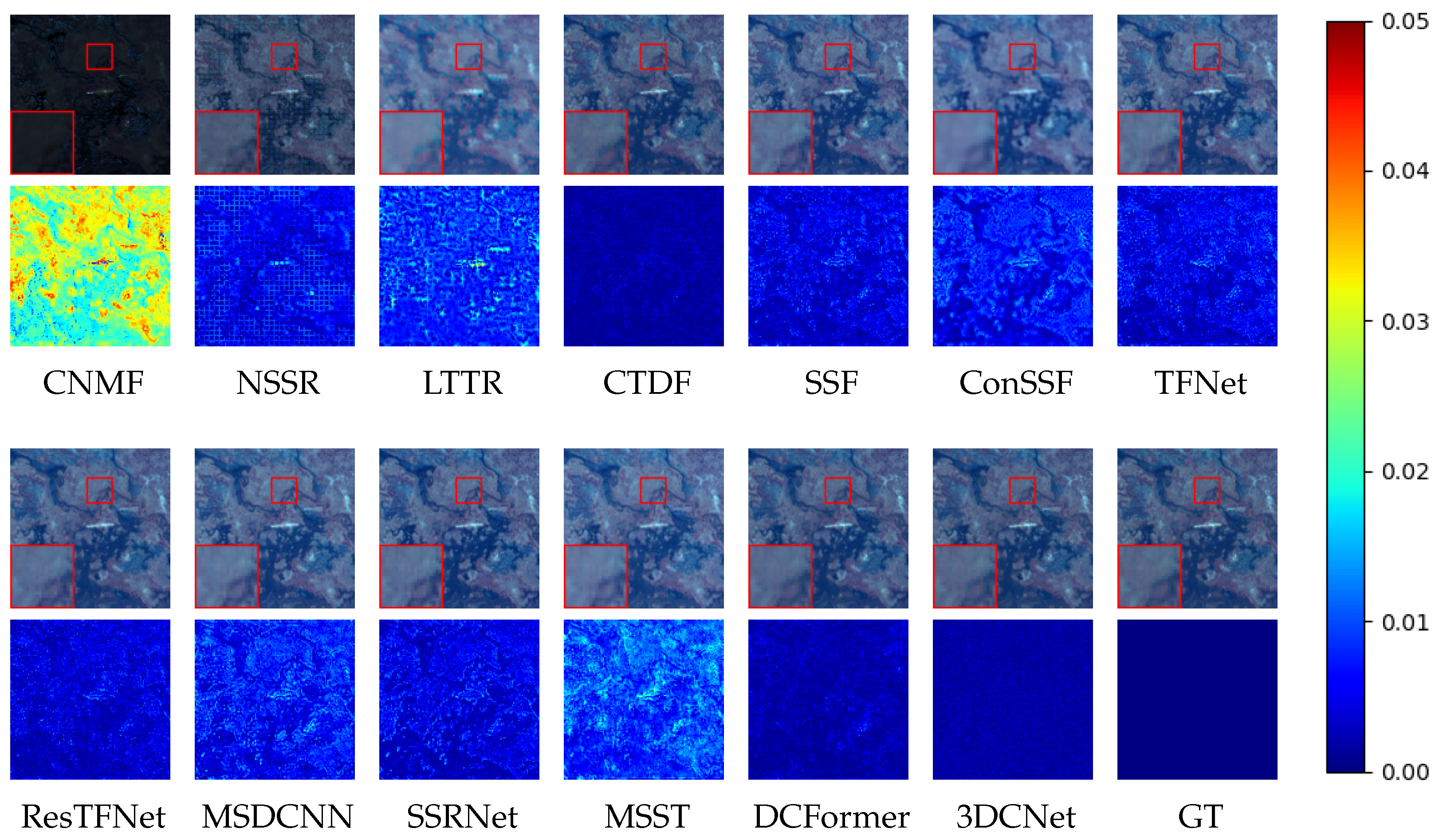
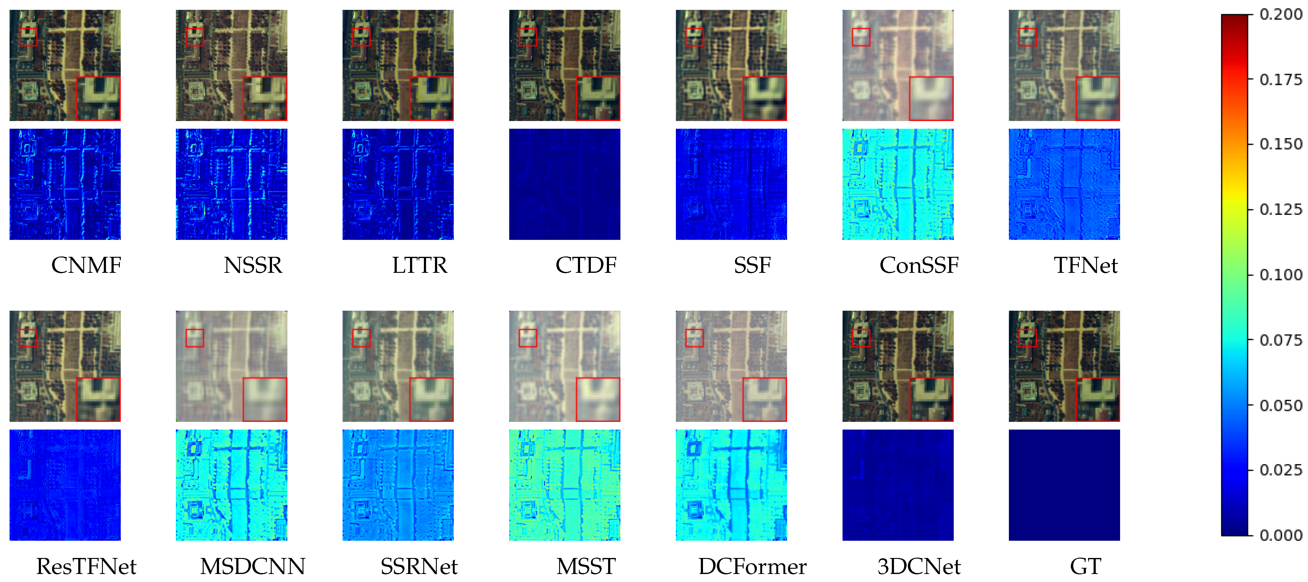
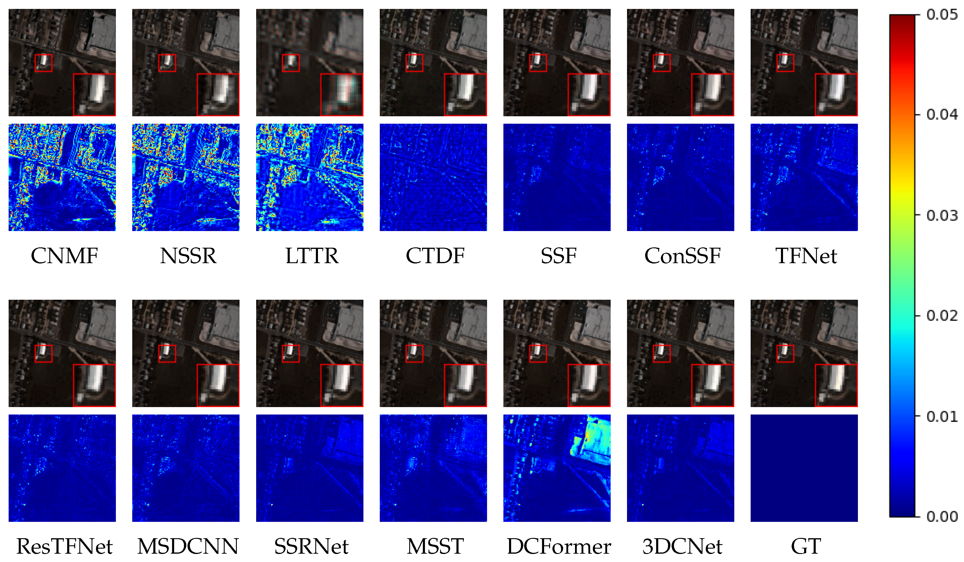
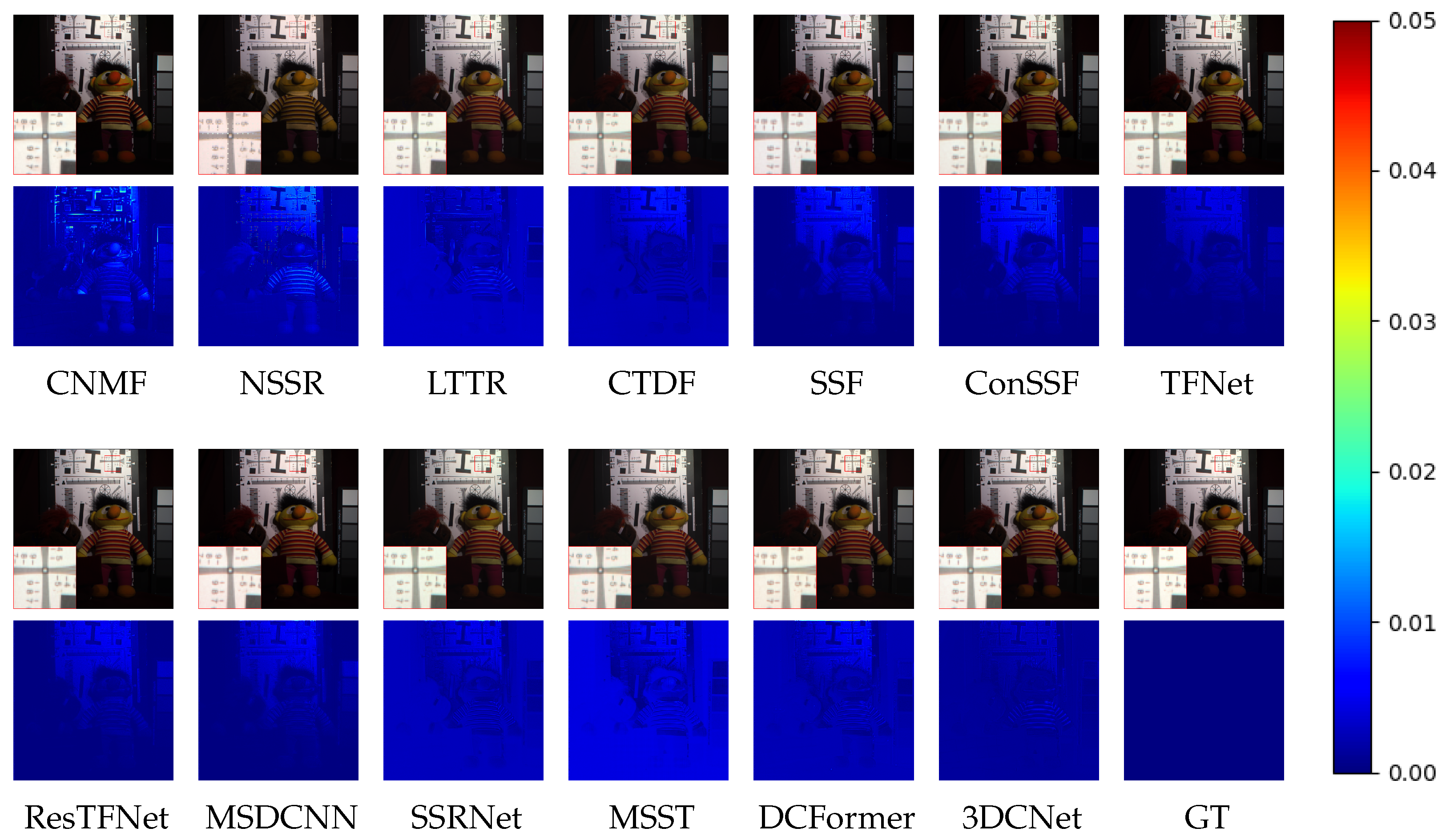
4.4. Fusion Performance Comparison

In this section, in order to verify the superiority of our 3DCNet, comparative experiments are conducted on the fusion performance of nine state-of-the-art methods on the Pavia University, Pavia Center, Indian Pines, Botswana, Washington DC Mall, and Urban datasets, both qualitatively and quantitatively. CNMF utilizes the matrix factorization-based method to synthesize HR-HSIs using an endmember matrix and a spatial abundance matrix. NSSR utilizes sparsity theory and leverages the spatial–spectral sparsity of HSIs by jointly learning a non-negative dictionary and estimating structured sparse codes to enhance image resolution. LTTR is a tensor decomposition-based method, and it learns the correlations among spatial and spectral modes considering nonlocal similarity, thereby achieving a super-resolution of the HSI. CTDF enhances feature extraction by representing a third-order HR-HSI with a higher-order spatial factor and a third-order spectral factor. The SSF method concatenates the HR-MSI and LR-HSI directly at the beginning of the network. ConSSF concatenates in the same way in each convolutional layer. TFNet utilizes the auto-encoder architecture to extract the spatial and spectral features separately. Skip connection is used in ResTFNet to learn deeper features. MSDCNN extracts information from different scales and different depths using convolutional layers and the residual learning trick. SSRNet designs a differential loss function and can achieve excellent performance using only three simple convolutional layers. MSST is a Transformer structure that incorporates masked band auto-encoders and masked patch auto-encoders, and it employs a self-supervised strategy to pre-train the network. DCFormer uses directional pairwise multi-head cross-attention to promote inter-modality information exchange, and the window attention mechanism is used to boost self-attention.

(1) Results on Pavia University: The quantitative comparison results are shown in

Table 2. The fusion results of the experimentally compared methods on the Pavia University dataset. The best scores are marked in red, and the second best scores are marked in blue.

Method	Pavia University
	RMSE	PSNR	ERGAS	SAM	SSIM
Best Value	0	$+\infty$	0	0	1
CNMF	11.047	26.951	5.431	10.758	0.845
NSSR	6.467	31.602	3.241	6.268	0.939
LTTR	4.994	33.846	2.505	4.279	0.948
CTDF	2.136	41.224	1.467	2.551	0.977
SSF	2.033	41.654	1.341	2.254	0.984
ConSSF	2.681	39.250	1.697	2.563	0.977
TFNet	2.313	40.533	1.518	2.487	0.979
ResTFNet	2.144	41.193	1.439	2.375	0.981
MSDCNN	2.432	40.097	1.581	2.671	0.980
SSRNet	1.756	42.928	1.175	1.996	0.987
MSST	2.833	38.772	1.788	2.767	0.976
DCFormer	2.666	39.298	1.614	2.079	0.986
3DCNet	1.601	43.729	1.101	1.885	0.988

, and the qualitative comparison RGB fusion results are shown in Figure 4. Based on Table 2, we can summarize that our 3DCNet outperforms all models in all metrics and that SSRNet ranks second only due to the detailed design of their loss functions. The better performance of ResTFNet than TFNet shows that residual connections can better help networks learn deep features. The better performance of our 3DCNet and SSRNet indicates that spatial and spectral loss functions play an important role in guiding networks during the training process. The MSST and DCFormer networks use a Transformer-based architecture, which requires more training data to support its large number of parameters. Therefore, their performance is not optimal on remote sensing images with limited data.

In Figure 4 and other comparison figures, it is worth noting that the first row shows the predicted RGB HR-HSIs of the algorithms or models and that the second row shows the difference RGB images between the predicted HR-HSIs and the reference HR-HSIs. The last column presents the ground truth. We can draw the conclusion that CNMF visually loses texture details. NSSR loses spatial resolution from the difference map. LTTR performs better, while it can still be seen in its difference map that there is a significant variation between it and the ground truth. We can observe from the difference image that CTDF performs relatively evenly across different areas of the image; however, overall, it introduces some noise. SSF achieves better performance than ConSSF, which indicates that the original image data introduced multiple times at different levels of depth may lead to the overfitting of the model.

(2) Results on Pavia Center:

Table 3. The fusion results of the experimentally compared methods on the Pavia Center dataset. The best scores are marked in red, and the second best scores are marked in blue.

Method	Pavia Center
	RMSE	PSNR	ERGAS	SAM	SSIM
Best Value	0	$+\infty$	0	0	1
CNMF	4.530	35.010	2.820	5.465	0.938
NSSR	3.643	36.901	2.396	4.438	0.964
LTTR	3.714	36.733	2.247	4.092	0.956
CTDF	2.158	41.449	1.789	3.398	0.970
SSF	1.818	42.941	1.545	2.725	0.981
ConSSF	5.015	34.125	3.341	6.061	0.964
TFNet	2.185	41.340	1.818	3.111	0.975
ResTFNet	1.988	42.163	1.708	2.927	0.977
MSDCNN	2.126	41.580	1.776	3.141	0.976
SSRNet	1.647	43.796	1.440	2.509	0.984
MSST	1.769	43.175	1.566	2.695	0.981
DCFormer	2.172	41.395	1.655	2.653	0.983
3DCNet	1.531	44.432	1.382	2.430	0.985

shows the quantitative results of all models on the Pavia Center dataset. It can be seen that the proposed 3DCNet performs best among all models. The same conclusion as that regarding the Pavia University dataset can be drawn due to the similarity of these two scenes, except for in terms of MSST. This is likely because it effectively extracts information from both hyperspectral and multispectral images during the pretraining phase. ConSSF still achieves the lowest performance metrics. CTDF outperforms other traditional methods, likely due to its connection through the fourth-order spatial factor and third-order spectral factor, which enables it to achieve enhanced feature extraction capabilities. In Figure 5, it can be seen that ConSSF achieves relatively better difference images. We speculate that the reason for this is that it performs well in the bands selected for display but shows poor performance in other bands. TFNet, ResTFNet, and MSDCNN exhibit slight pixel distortion. However, our 3DCNet results in the minimal loss.

(3) Results on Indian Pines: As demonstrated in

Table 4. The fusion results of the experimentally compared methods on the Indian Pines dataset. The best scores are marked in red, and the second best scores are marked in blue.

Method	Indian Pines
	RMSE	PSNR	ERGAS	SAM	SSIM
Best Value	0	$+\infty$	0	0	1
CNMF	5.038	34.085	2.475	4.480	0.770
NSSR	5.168	33.865	2.536	4.238	0.780
LTTR	4.695	34.699	2.308	4.607	0.777
CTDF	3.237	37.062	1.387	2.508	0.946
SSF	9.272	28.787	9.784	7.582	0.838
ConSSF	7.623	30.489	15.587	5.949	0.612
TFNet	5.515	33.301	2.673	3.799	0.917
ResTFNet	5.203	33.806	2.615	3.611	0.923
MSDCNN	5.355	33.556	2.832	3.763	0.917
SSRNet	5.028	34.103	7.977	3.598	0.874
MSST	5.099	33.115	2.450	3.476	0.922
DCFormer	4.191	34.817	1.619	2.806	0.945
3DCNet	2.679	38.706	1.599	1.997	0.970

, 3DCNet and CTDF perform the best and second best, respectively, surpassing all other models in all metrics. However, the former has a worse ERGAS than the latter, indicating that the former’s detail features and texture information still need further improvement. Other traditional methods achieve comparable or even better results than deep learning methods, suggesting that CNMF captures both the local and global information of the dataset effectively. NSSR finds a better sparse representation for this dataset. LTTR also effectively captures and utilizes spatial and spectral similarity information. However, SSF and ConSSF overall perform noticeably worse than the other models, indicating that simple models, if not equipped with well-designed loss functions, lead to underfitting.

The RGB and difference maps in Figure 6 reveal that, although SSF achieves worse metrics, its RGB image is clearer than LTTR’s, and its difference image shows smaller errors compared to LTTR. This indicates that it is not enough to evaluate a model solely based on metrics. From the RGB images, it is clear that CNMF, CTDF, and our 3DCNet capture more texture information.

(4) Results on Botswana: The quantitative results of our 3DCNet and other comparative methods on the Botswana dataset are presented in

Table 5. The fusion results of the experimentally compared methods on the Botswana dataset. The best scores are marked in red, and the second best scores are marked in blue.

Method	Botswana
	RMSE	PSNR	ERGAS	SAM	SSIM
Best Value	0	$+\infty$	0	0	1
CNMF	2.166	26.444	7.787	8.903	0.832
NSSR	1.025	32.945	3.640	5.764	0.864
LTTR	0.817	34.919	2.808	6.943	0.866
CTDF	0.396	39.275	2.682	1.923	0.998
SSF	0.843	34.645	11.509	4.322	0.982
ConSSF	1.095	32.368	15.277	4.865	0.960
TFNet	0.521	38.821	3.198	2.579	0.997
ResTFNet	0.469	39.743	2.981	2.368	0.997
MSDCNN	0.591	37.730	3.602	2.928	0.996
SSRNet	0.522	38.809	6.719	2.657	0.992
MSST	0.683	34.533	3.000	2.620	0.995
DCFormer	0.352	40.292	2.538	1.617	0.998
3DCNet	0.319	42.521	2.474	1.523	0.998

. It is evident that, overall, our 3DCNet outperforms other models on this dataset. For the Botswana dataset, which has a relative substantial number of training samples, the residual connections enable ResTFNet to better capture deep features compared to TFNet, thus producing superior results. The outcomes of MSDCNN demonstrate that multiscale and multidepth CNNs are not sufficient. Moreover, the inferior results of ConSSF compared to those of SSF suggest that injecting shallow-layer information into subsequent layers via residual connections can lead to insufficient feature learning if the integration point is not properly selected. As observed in Figure 7, CNMF clearly fails to learn the characteristics of this dataset. The RGB images of LTTR and ConSSF appear brighter, indicating a significant deviation from the reference images. The difference maps of MSST and DCFormer show that window attention can capture more details when using a Transformer-based architecture.

(5) Results on Washington DC Mall: The experimental results of all models are shown quantitatively in

Table 6. The fusion results of the experimentally compared methods on the Washington DC Mall dataset. The best scores are marked in red, and the second best scores are marked in blue.

Method	Washington DC Mall
	RMSE	PSNR	ERGAS	SAM	SSIM
Best Value	0	$+\infty$	0	0	1
CNMF	0.954	45.879	0.175	0.308	0.995
NSSR	2.708	36.814	0.497	0.848	0.958
LTTR	1.356	42.825	0.249	0.358	0.985
CTDF	1.263	43.442	0.230	0.514	0.983
SSF	19.545	19.646	3.639	8.220	0.941
ConSSF	13.611	22.789	2.602	5.701	0.933
TFNet	1.923	39.786	0.337	0.646	0.969
ResTFNet	1.824	40.249	0.319	0.613	0.973
MSDCNN	3.056	35.765	0.535	1.009	0.928
SSRNet	2.291	38.266	0.401	0.801	0.957
MSST	2.372	37.964	0.413	0.738	0.953
DCFormer	1.550	41.659	0.278	0.541	0.992
3DCNet	0.830	47.083	0.148	0.301	0.995

and qualitatively in Figure 8. Our 3DCNet ranks first in terms of all metrics. However, CNMF shows that alternating nonnegative matrix factorization algorithms can fully extract spatial and spectral information on the Washington DC Mall dataset. LTTR shows that nonlocal similarity has the potential to preserve the visual message in terms of the SSIM metric. We can see that ConSSF and SSF exhibit relatively large fluctuations in performance across different datasets. Moreover, 3DCNet uses a loss function similar to SSRNet, but its more complex and refined network architecture allows it to outperform the latter by a large margin. CTDF still performs stably, but the method of mapping data to higher dimensions may lead to convergence to a local optimum. In Figure 8, the difference results reveal that ConSSF and MSDCNN fail to show robust generalization. Moreover, the iterative integration of HSI and MSI data and the application of multi-scale convolutional layers within their fusion strategies do not have the desired effects. From the RGB images, it can be observed that NSSR, TFNet, ResTFNet, and SSRNet produce brighter images, indicating that these methods do not capture the luminance and color information effectively. DCFormer exhibits more detailed texture information than MSST, suggesting that the window attention mechanism is more capable of capturing local details.

(6) Results on Urban:

Table 7. The fusion results of the experimentally compared methods on the Urban dataset. The best scores are marked in red, and the second best scores are marked in blue.

Method	Urban
	RMSE	PSNR	ERGAS	SAM	SSIM
Best Value	0	$+\infty$	0	0	1
CNMF	7.133	28.818	3.621	8.083	0.923
NSSR	6.120	30.148	3.105	6.459	0.950
LTTR	7.024	28.952	3.575	6.839	0.911
CTDF	2.276	38.741	1.391	2.666	0.988
SSF	9.032	26.767	4.696	8.796	0.963
ConSSF	3.951	33.948	1.971	3.236	0.972
TFNet	3.127	35.979	1.763	2.957	0.983
ResTFNet	2.947	36.496	1.623	2.738	0.984
MSDCNN	2.966	36.438	1.692	2.992	0.983
SSRNet	2.483	37.985	1.280	2.455	0.988
MSST	3.460	35.102	1.904	3.133	0.977
DCFormer	3.747	34.410	2.121	2.063	0.987
3DCNet	2.062	39.598	1.079	2.062	0.991

lists the experimental results of our 3DCNet and other comparative methods. The proposed 3DCNet obtains the best performance among all models in all metrics, thus demonstrating overall superiority. SSRNet ranks second for all metrics, showing the validity of the elaborate design of its loss function. The better performance of our 3DCNet than SSRNet demonstrates the advantage of using different branches to seperately extract features. CTDF achieves the second-best results in the RMSE, PSNR, and SSIM, indicating that the CTDF method handles pixel-level details better but overlooks the structural and global consistency of the image. In contrast, SSRNet performs better in terms of image structure. Furthermore, MSDCNN and ResTFNet outperform MSST and DCFormer overall, suggesting that convolutional operations perform better than Transformers on datasets with limited data. Figure 9 shows that CNMF, NSSR, and LTTR lose more spatial information due to their blurry output HR-HSIs and their difference images. When we zoom in on the difference images, we can see that, although DCFormer performs well on average in terms of RGB images, the variance in fluctuations at each pixel compared to the reference image is relatively large.

(7) Results on CAVE: In

Table 8. The fusion results of the experimentally compared methods on the Cave dataset. The best scores are marked in red, and the second best scores are marked in blue.

Method	CAVE
	RMSE	PSNR	ERGAS	SAM	SSIM
Best Value	0	$+\infty$	0	0	1
CNMF	5.493	33.436	3.484	13.848	0.927
NSSR	5.962	34.529	4.871	10.332	0.965
LTTR	1.898	44.597	1.321	4.163	0.992
CTDF	1.556	46.067	1.127	3.624	0.992
SSF	2.062	42.346	1.306	3.198	0.992
ConSSF	1.777	43.977	1.105	2.801	0.994
TFNet	1.531	45.169	0.963	3.017	0.995
ResTFNet	1.338	45.980	0.850	2.917	0.995
MSDCNN	1.629	44.402	1.031	2.992	0.995
SSRNet	1.860	43.646	1.246	3.268	0.995
MSST	1.623	45.845	1.161	3.786	0.990
DCFormer	2.326	41.357	1.480	3.460	0.991
3DCNet	1.446	46.092	0.916	2.998	0.994

, we can see the weakness of our 3DCNet when it is applied with fewer bands. Its performance does not reach the best level but still achieves second place. This could be because fewer bands imply a lack of training data, and the shallower network depth of 3DCNet means that it cannot extract deeper high-dimensional features. In contrast, ResTFNet, although simpler in network structure and training approach, benefits from its deeper network layers and residual connections, which allow it to capture deeper information more effectively. ConSSF performs well on the SAM and SSIM metrics, indicating its strong ability to capture global information. In Figure 10, it can be seen that the RGB images of NSSR and MSDCNN have a reddish tint, while SSRNet exhibits a blackish tint. This indicates that these models fail to maintain the original color balance during the image reconstruction process, leading to the reddish or blackish color bias. Although 3DCNet does not achieve better metrics, its difference image suggests that it performs better than ResTFNet in terms of detail recovery.

To sum up, the proposed 3DCNet shows the best fusion performance on seven datasets. Deep learning methods do not always show superiority to traditional methods, with this depending on the careful design of the information extraction method. The advantages of feeding data to the model all in one stage, using residual connection structures, and carefully designing loss functions are apparent. Although all other methods may perform excellently on specific datasets, 3DCNet excels due to its strong generalization ability and stable performance across various metrics.

4.5. Downstream Classification Performance Comparison

In this subsection, we compare the performance of downstream classification applications on fused images generated by various deep learning-based fusion methods on four datasets: the Pavia University, Pavia Center, Indian Pines, and Botswana datasets. All the classes in the testing area are ordered in

Table 9. Class labels for different datasets. The classes for each dataset are listed in the order shown in tables below.

Dataset	Class
Pavia University	asphalt, meadows, trees, painted metal sheets, bare soil, bitumen, self-blocking bricks, shadows
Pavia	water, trees, asphalt, self-blocking bricks, bitumen, tiles, bare soil
Indian Pines	corn-notill, corn-mintill, corn, grass-pasture, grass-trees, oats, soybean-notill, soybean-mintill, soybean-clean, buildings-grass-trees-drives, stone-steel-towers
Botswana	water, hippo grass, reeds 1, firescar 2, Acacia woodlands, exposed soils

. DBDA [18] is utilized as the classification network. Initially, we apply the ATIS solely to our 3DCNet, iteratively refining both the fusion and classification networks. The quantitative classification results on the Pavia University dataset are presented in

Table 10. The results of the downstream classification experiments on the Pavia University dataset using 1% of available labeled data. ATIS is only applied to our 3DCNet, and other models directly train the classification models. The best scores are marked in red.

Class	Count	SSF	ConSS	TFNet	ResTF	MSD	SSR	MSST	DCFor	Ours
1	365	100.0	89.59	100.0	94.80	98.08	96.71	98.36	96.99	100.0
2	570	100.0	100.0	99.83	100.0	100.0	100.00	100.0	100.0	100.0
3	114	0	0	0	0	0	0	0	0	100.0
4	580	95.86	100.0	98.62	100.0	100.0	98.83	100.0	100.0	100.0
5	3537	40.43	50.75	37.04	36.53	36.87	54.82	56.63	43.99	100.0
6	753	0	0	0	0	0	0	0	0	94.42
7	52	100.0	100.0	100.0	100.0	100.0	100.0	100.0	100.0	94.23
8	233	0	0	0	0	0	0	0	0	92.70
OA		47.92	53.58	46.23	45.78	46.16	56.30	57.45	50.16	99.00
AA		54.54	55.04	54.44	53.92	54.37	56.30	56.87	55.12	97.67
KAPPA		35.95	41.01	34.68	34.38	34.54	43.35	44.90	38.09	98.43

. It is important to note that our statistics on classification accuracy for each category, as well as the metrics OA, AA, and KAPPA, are based on the testing area. It is evident that our 3DCNet, enhanced by the ATIS, achieves the highest OA, AA, and KAPPA within the test area, and the prediction accuracy for each category reaches above 90%. Other deep learning models fail to predict any samples of trees, bitumen, and shadows. This may be attributed to the fact that, for these categories, the small number of training samples shows significant variation along the spectral dimension, which hinders the classification model from acquiring any meaningful knowledge. This observation indicates that, despite Figure 4 showing minimal visual differences in the predictions of all models, tiny variations can lead to significant prediction biases for downstream classification neural networks. The significant role of the ATIS in iteratively converging the two networks to generate images is thus highlighted. Consequently, in the subsequent comparative experiments for the downstream classification application, we employ the ATIS to iterate over all fusion networks.

(1) Results on Pavia University: Even though all deep learning fusion models employ the ATIS, our 3DCNet, due to its superior performance in various aspects, is capable of generating images that closely resemble the reference while ensuring that the spectral curves of samples in the same category are more similar. The visual results of classification using the ATIS on the Pavia University dataset are shown in Figure 11, with the quantitative results presented in

Table 11. The results of the downstream classification experiments on the Pavia University dataset using 1% of the available labeled data. The best scores are marked in red, and the second best scores are marked in blue.

Class	Count	SSF	ConSS	TFNet	ResTF	MSD	SSR	MSST	DCFor	Ours
1	365	100.0	100.0	100.0	100.0	100.0	100.0	100.0	100.0	100.0
2	570	97.19	100.0	84.74	100.0	100.0	100.0	96.67	97.72	100.0
3	114	100.0	100.0	100.0	100.0	100.0	100.0	100.0	100.0	100.0
4	580	100.0	100.0	100.0	100.0	100.0	98.45	100.0	100.0	100.0
5	3537	72.75	85.58	61.86	37.38	66.64	96.16	86.32	88.01	100.0
6	753	84.46	87.12	63.88	81.54	87.65	73.71	94.16	90.44	94.42
7	52	100.0	100.0	100.0	100.0	100.0	100.0	100.0	100.0	94.23
8	233	99.57	99.14	98.71	98.71	99.57	88.41	95.28	93.99	92.70
OA		82.30	90.18	72.42	62.01	79.47	94.04	91.01	91.57	99.00
AA		94.25	96.48	88.65	89.70	94.23	94.59	96.55	96.27	97.67
KAPPA		75.15	85.53	62.66	53.06	71.89	90.83	86.66	87.43	98.43

. The color of the classification results can be known in DBDA [18]. The visual results clearly demonstrate that the downstream classification outcomes of our 3DCNet are the closest to the ground truth, followed by SSRNet, whereas other deep learning models misclassify a significant number of samples, particularly in the bare soil category. The quantitative results indicate that our 3DCNet achieves the highest OA, AA, and KAPPA, and the classification accuracy for all categories is beyond 90%, even near 100%. Upon examining the classification outcomes of SSF, ConSSF, TFNet, ResTFNet, and MSDCNN after the application of the ATIS, it is evident that the prediction accuracies for the two most abundant categories, bare soil and bitumen, are not high, which also explains their relatively lower OAs. Although the fusion results of MSST and DCFormer are slightly inferior, through multiple rounds of iterative training on the fusion and classification networks, they obtain sufficient training data, thereby achieving relatively optimal classification performance. The highest KAPPA achieved by 3DCNet indicates the highest level of consistency in the downstream classification outcomes. SSRNet, which similarly utilizes the image edge extraction loss function, achieves results close to those of 3DCNet, thereby indirectly validating the effectiveness of the Canny operator employed by 3DCNet.

(2) Results on Pavia Center: The classification results after the application of the ATIS on various models on the Pavia Center dataset are presented in

Table 12. The results of the downstream classification experiments on the Pavia Center dataset using 0.5% of the available labeled data. The best scores are marked in red, and the second best scores are marked in blue.

Class	Count	SSF	ConSS	TFNet	ResTF	MSD	SSR	MSST	DCFor	Ours
1	563	100.0	100.0	100.0	100.0	100.0	100.0	100.0	100.0	100.0
2	41	19.51	58.54	46.34	19.51	19.51	60.98	100.0	100.0	97.56
3	327	99.69	99.69	74.62	100.0	85.93	73.09	52.60	45.87	66.36
4	524	43.70	50.57	60.12	58.78	75.38	93.89	99.24	100.0	97.71
5	3437	99.97	100.0	99.80	99.51	100.0	99.94	100.0	100.0	100.0
6	635	100.0	100.0	98.27	100.0	100.0	99.84	100.0	100.0	100.0
7	24	100.0	100.0	100.0	100.0	100.0	100.0	100.0	100.0	100.0
OA		94.06	95.01	94.02	95.21	96.25	97.46	97.14	96.81	97.78
AA		80.41	86.97	82.73	82.54	82.98	89.68	93.12	92.27	94.52
KAPPA		89.24	91.03	89.19	91.47	93.35	95.54	94.95	94.34	96.10

. The quantitative results show that, for the most abundant category within the test area, bitumen, all models achieve an accuracy rate of over 99%; thus, all attained OAs of more than 90%. Regarding the asphalt category, although our 3DCNet has a lower prediction accuracy, it still surpasses MSST and DCFormer. Overall, our 3DCNet achieves the highest OA, AA, and KAPPA, demonstrating that, under the ATIS strategy, 3DCNet can perform more effectively with better convergence of both the fusion and classification models, and MSST follows closely. The lower AAs of the other models suggests that their prediction accuracy for different category samples is not stable.

(3) Results on Indian Pines: The classification results of 3DCNet and the other deep learning models on the Indian Pines dataset after employing the ATIS are presented in

Table 13. The results of the downstream classification experiments on the Indian Pines dataset using 5% of the available labeled data. The best scores are marked in red, and the second best scores are marked in blue.

Class	Count	SSF	ConSS	TFNet	ResTF	MSD	SSR	MSST	DCFor	Ours
1	732	96.45	89.21	93.58	94.95	97.81	98.09	98.63	93.44	93.44
2	434	85.95	99.08	99.08	99.77	97.47	98.85	94.70	91.48	98.16
3	237	67.09	73.84	63.29	88.19	79.75	73.00	85.23	80.17	83.12
4	18	0	0	0	0	0	0	0	0	0
5	190	100.0	98.95	100.0	100.0	100.0	99.47	99.47	99.47	94.21
6	6	66.67	66.67	100.0	100.0	83.33	100.0	100.0	100.0	100.0
7	60	21.67	40.00	40.00	68.33	80.00	46.67	61.67	61.67	66.67
8	252	82.94	84.13	98.41	88.89	78.97	59.13	53.18	94.05	93.25
9	510	91.37	81.37	80.39	54.90	84.31	87.06	85.69	82.55	82.75
10	89	100.0	98.88	95.51	89.89	95.51	97.75	92.14	95.51	95.51
11	93	95.67	100.0	95.70	100.0	94.62	97.85	100.0	100.0	98.93
OA		87.67	87.07	88.40	85.88	90.54	88.29	88.25	89.24	90.27
AA		73.44	75.65	78.72	80.45	81.07	77.99	79.16	81.67	82.37
KAPPA		85.06	84.48	86.02	83.07	88.62	85.85	85.75	87.09	88.34

. Overall, our 3DCNet ranks first place in AA and second in terms of both OA and KAPPA, with a narrow margin behind MSDCNN. Despite its relatively poor fusion performance, the superior classification performance of MSDCNN on this dataset may be attributed to the ATIS making the fusion model and the classification model further converge. Moreover, the generally lower AAs achieved by all models on the Indian Pines dataset may be due to the fact that, within the prediction area, the grass-pasture category, although only consisting of 18 sample points, is not correctly predicted by any model. This is probably because the downstream classification DBDA network is sensitive to the spectral curve variations in the grass-pasture category. Compared to SSRNet and 3DCNet, SSF and ConSSF achieve poorer results, which suggests that simple fusion models, without the use of well-designed loss functions, cannot achieve satisfactory convergence effects given the condition of a small number of samples, thus leading to a lower accuracy in downstream classification applications. In contrast, TFNet and ResTFNet utilize deeper and more complex network architectures, enhancing the models’ representational capacity to some degree. MSST and DCFormer have the same condition as TFNet and ResTFNet.

(4) Results on Botswana: The results of the downstream classification application on the Botswana dataset are presented in

Table 14. The results of the downstream classification experiments on the Botswana dataset using 3% of the available labeled data. The best scores are marked in red, and the second best scores are marked in blue.

Class	Count	SSF	ConSS	TFNet	ResTF	MSD	SSR	MSST	DCFor	Ours
1	34	100.0	100.0	100.0	100.0	97.06	100.0	100.0	100.0	100.0
2	58	100.0	100.0	89.66	86.21	100.0	98.28	100.0	86.21	100.0
3	3	0	0	100.0	0	100.0	100.0	100.0	100.0	100.0
4	43	100.0	100.0	100.0	100.0	100.0	100.0	100.0	100.0	100.0
5	33	100.0	100.0	100.0	100.0	100.0	100.0	100.0	100.0	100.0
6	16	62.50	43.75	0.00	50.00	62.50	37.50	62.50	87.50	87.50
OA		95.19	93.58	88.24	89.84	91.44	94.12	96.79	94.65	98.93
AA		77.08	73.96	81.61	72.70	83.89	89.30	93.75	95.62	97.92
KAPPA		93.80	91.77	85.21	87.23	89.09	92.51	95.90	93.26	98.63

. It should be noted that the distribution of the categories in Botswana is relatively dispersed. We specifically select the test area mentioned in Table 1 to cover as many categories as possible, thereby sacrificing the count of samples per category. Compared to other datasets, all models exhibit better classification performance on the Botswana dataset in terms of OA, AA, and KAPPA. However, SSF, ConSSF, and ResTFNet still achieve a prediction accuracy of 0% for the reeds 1 category, leading to their relatively lower AAs. SSF has a large improvement in both OA and KAPPA, which may imply that, although the fused images generated by SSF are not of high quality, they retain deep spectral characteristics that can be used in the classification process. This could also be attributed to the small sample size of the test area in the Botswana dataset, resulting in large variability in the results. Our 3DCNet achieves nearly 100% prediction accuracy in almost all categories, except for the exposed soils category, which also verifies that our 3DCNet, in conjunction with the ATIS strategy, can be applied to datasets with varying conditions.

In summary, 3DCNet achieves the best classification results across the four datasets. This is mainly attributed to the quality of the fused HR-HSI generated by the fusion networks. The higher the fusion assessment metrics of the generated images, the more the details that can be captured and the more faithfully they reproduce the spectral curves, which further confirms the conclusions of our fusion experiments.

4.6. Ablation Experiments

In this section, we first study the significance of various components in our 3DCNet on the Urban dataset, followed by the impact of different elements of the alternating training iteration strategy (ATIS) on the Pavia University dataset. Finally, another classification model, 3DCFormer [51], is used to validate the effectiveness of the ATIS.

(1) 3DCNet Ablation Experiments: As depicted in

Table 15. Ablation experiments of the proposed 3DCNet on the Urban dataset. The best data are marked in red.

Strategy	Urban Ablation Experiment
	RMSE	PSNR	ERGAS	SAM	SSIM
w/o-spat	2.547	37.762	1.249	2.580	0.987
w/o-spec	2.302	38.641	1.152	2.291	0.989
w/o-2stream	2.264	38.787	1.174	2.252	0.990
w/o-canny	2.358	38.433	1.179	2.135	0.990
w/o-angle	2.147	39.245	1.124	2.126	0.990
3DCNet	2.062	39.598	1.079	2.062	0.991

, the term w/o-spat, short for without spatial, signifies the removal of every SpatB as well as ${\mathcal{L}}_{canny}$ from the network. Similarly, w/o-spec denotes the absence of all SpecB and ${\mathcal{L}}_{angle}$. W/o-2stream indicates the elimination of the $\mathbf{X}$ and $\mathbf{Y}$ branches from the 3DCNet model. The terms w/o-canny or w/o-angle represent the exclusion of only ${\mathcal{L}}_{canny}$ or ${\mathcal{L}}_{angle}$ from the loss function, respectively.

The findings reveal that all these components utilized are instrumental in the superior performance of 3DCNet. Notably, the absence of the SpatB significantly affects all metrics, emphasizing its role in capturing fine-grained spatial details. A comparative analysis between the scenarios of w/o-canny versus w/o-angle, and w/o-spat versus w/o-spec suggests that reconstructing the spatial information of the HR-HSI is more challenging than the spectral information within the Urban dataset.

It is also noteworthy that the w/o-2stream ablation experiment utilizes the same single-stream feature extraction network as SSRNet, thereby highlighting the effectiveness of our three-stream information extraction network in generating HR-HSIs. A thorough comparison of the outcomes from all these ablation architectures to the loss functions, along with input data, proves that 3DCNet’s excellence is a result of its multiple advantageous components.

(2) ATIS Ablation Experiments on Classification results: As shown in

Table 16. Ablation experiments of our ATIS on the Pavia University dataset. The best scores are marked in red, and the second best scores are marked in blue.

Strategy	Class								Metric
	1	2	3	4	5	6	7	8	OA	AA	KAPPA
classification on the reference	100.0	100.0	100.0	100.0	98.90	95.88	100.0	99.57	98.86	99.29	98.22
transferred classification model	100.0	100.0	100.0	100.0	80.24	82.74	100.0	99.57	86.62	95.32	80.70
one stage training	88.49	100.0	95.61	92.24	73.40	0	100.0	0	67.46	68.72	54.89
without loss interaction	100.0	93.33	100.0	100.0	93.36	97.74	92.31	89.70	94.87	95.81	92.15
our ATIS	100.0	100.0	100.0	100.0	100.0	94.42	94.23	92.70	99.00	97.67	98.43

, the baseline for our study is established by classification on the reference strategy, where the classification network is trained directly on the reference HR-HSI. Notably, our implementation of the DBDA [18] network achieves results surpassing those of the original paper due to an increased training sample set. The transferred classification model strategy denotes the use of a model pretrained on the reference HR-HSI without further adaptation to the fused images produced by 3DCNet, while the one-stage training strategy reflects a non-iterative approach. The without loss interaction row illustrates the impact of disabling loss function communication during the alternating training of the fusion and classification networks, setting $n=0$ throughout Algorithm 1.

The results clearly show that the OA, AA, and KAPPA metrics of our ATIS closely match those of classification on the reference strategy, indicating that the ATIS effectively refines the fused images to better serve the downstream classification task. We can observe that, after employing the ATIS strategy, our classification performance surprisingly surpasses the strategy of classification on the reference image. However, this does not guarantee that our method outperforms direct classification on the reference image for every individual category. This result falls within the acceptable margin of error. It is attributed to the overall performance improvement caused by the bare soil category, which has the largest number of samples, being predicted entirely correctly. The outcome of the transferred classification model strategy highlights the significant deviation between the fused HR-HSI generated by the fusion network and the reference HR-HSI, so the retraining of the classification network on the fused images is necessary. Furthermore, a comparison between the one-stage training strategy and our ATIS reveals that the initial fused images must undergo multiple iterative refinements to enhance their utility for classification. The without loss interaction scenario, where there is no information exchange between the training processes of the fusion and classification networks, leads to slightly inferior results.

Thus, it can be concluded that our ATIS integrates all the aforementioned elements: it trains the classification network on the generated fused HR-HSI, employs multiple iterations, and maintains information exchange between the two networks during the iteration process. Consequently, the downstream classification results achieved with the ATIS are the best.

(3) ATIS Ablation Experiments on Fusion results: We conduct ablation studies on the Pavia University dataset to observe the impact of the ATIS on the fusion results, as shown in

Table 17. The impact of the ATIS on the fusion results on the Pavia University dataset. The best scores are marked in red, and the second best scores are marked in blue.

Strategy	Pavia University
	RMSE	PSNR	ERGAS	SAM	SSIM
one-stage	1.777	43.139	1.375	1.993	0.986
ATIS	1.645	43.491	1.131	1.899	0.987
only fusion	1.601	43.729	1.101	1.885	0.988

. It can be seen that, when only the fusion task is considered, all fusion metrics reach their optimal values. However, using a one-stage ATIS framework, where the classification loss is incorporated into the fusion task only once, leads to a noticeable decline in fusion performance. However, with the full ATIS framework, which iteratively incorporates the classification loss into the fusion network and the fusion loss into the classification network, the results show some improvement but still fall short of the performance achieved by using the fusion network alone. It is worth noting that, although the ATIS has a slight impact on the fusion results, it still outperforms the other comparison methods shown in Table 2.

(4) Classification Model Ablation Experiments: Another classification model, 3DCFormer [51], is utilized to validate the effectiveness of the ATIS. We fix the upstream fusion network as our 3DCNet while replacing the downstream classification network from DBDA to 3DCFormer. All other settings remain the same. The generalization ability of the ATIS is verified sequentially on four datasets: the Pavia University, Pavia Center, Indian Pines, and Botswana datasets. The results are presented in

Table 18. Classification results of our fusion model 3DCNet and downstream classification model DBDA or 3DCFormer using the ATIS. The best scores are shown in red.

Dataset	OA		AA		KAPPA
	3DCFormer	DBDA	3DCFormer	DBDA	3DCFormer	DBDA
Pavia University	97.10	99.00	99.16	97.67	95.54	98.43
Pavia Center	98.58	97.78	96.78	94.52	98.46	96.10
Indian Pines	89.62	90.27	80.07	82.37	91.17	88.34
Botswana	99.47	98.93	99.71	97.92	97.33	98.63

. The results show that the ATIS is not only applicable to the classification model DBDA but also works well with other classification models.

4.7. Efficiency Experiments

While deep learning methods can build highly complex models that achieve excellent performance, the huge number of parameters often hampers their deployment, and the long inference time renders them impractical for real-time applications. This section evaluates the computational complexity of deep-learning models on the Urban dataset through three key metrics: the number of parameters, floating-point operations, and testing time. The detailed data are presented in

Table 19. Model complexity of the proposed 3DCNet and other deep learning models. The best data are marked in red, and the second best data are marked in blue.

Model	Urban Complexity Experiment
	Params (M)	FLOPs (G)	Testing (ms)
SSF	1.136	37.217	174
ConSSF	1.163	38.119	115
TFNet	2.501	19.891	159
ResTFNet	2.376	18.618	111
MSDCNN	1.823	59.741	177
SSRNet	0.709	23.219	41
MSST	41.01	527.58	464
DCFormer	5.410	318.51	294
3DCNet	0.708	15.923	94

. It should be noted that all models are tested on the testing area specified in Table 1.

According to the quantitative data, our 3DCNet ranks first on parameters and FLOPs and second for testing time. While SSRNet has a parameter count close to that of our 3DCNet, its FLOPs are 1.46 times higher, demanding greater computational resources. Although ResTFNet has the second-lowest FLOPs, its larger number of parameters and longer testing time increase its deployment barrier and decrease its suitability for real-time applications. MSST and DCFormer have a large number of parameters, resulting in the highest FLOPs and testing time. This makes it difficult to deploy them on edge devices and challenging to meet real-time requirements. It is important to note that, despite our 3DCNet having the fewest parameters and FLOPs, the low-cost linear transformation operations within the SpatB result in frequent memory access, which significantly increases the testing time. Consequently, the testing time of 3DCNet is 1.3 times longer than that of SSRNet, but it still ranks as the second fastest.

4.8. Hyperparameter Sensitivity Analysis

The training process involves many hyperparameters, and the values of these hyperparameters are crucial for the convergence of the network. We select the four most important hyperparameters for this experiment to conduct a hyperparameter analysis. These include the coefficients of the different loss functions, as well as the initial learning rate. As shown in Figure 12, the PSNR values corresponding to the coefficients of the loss functions are on the left side of the plot, while the PSNR values corresponding to the learning rates are on the right side. With the other parameters kept constant, we conduct 20 experiments for ${\lambda }_1$, and the results are shown by the blue line. It can be seen that, as ${\lambda }_1$ increases, the PSNR value of the fused image generally rises first and then decreases. From the black and orange lines, it is clear that, as ${\lambda }_2$ or ${\lambda }_3$ increases, the PSNR value of the fused image gradually decreases. The red line represents the choice of the initial learning rates, specifically ${10}^{-1}$, ${10}^{-2}$, ${10}^{-3}$, ${10}^{-4}$, and ${10}^{-5}$. Since a learning rate that is too high may prevent the model from converging, we decrease the learning rate gradually in the training process to maintain training stability. Even so, we observe that the choice of the initial learning rate has a significant impact on the convergence of the model. Only when the learning rate is ${10}^{-3}$ is the model able to find the global optimal region early in training, gradually approaching the optimal value in the later stages. Higher learning rates cause parameter oscillations, which may miss the global optimum, while lower learning rates result in the parameters staying close to the initial values, preventing the model from reaching the optimal region. In conclusion, the selection of these hyperparameters in this study is both reasonable and meaningful.

5. Conclusions

This paper presents a novel HSI and MSI fusion framework, the three-stream fusion network for downstream classification application (3DCNet), designed to generate HR-HSIs from LR-HSIs and HR-MSIs. The SpatB and SpecB are designed to effectively extract spatial and spectral features, respectively. The loss functions ${\mathcal{L}}_{canny}$ and ${\mathcal{L}}_{angle}$ are utilized to guide the learning process of spatial and spectral features. The proposed 3DCNet framework has been extensively evaluated and compared with state-of-the-art methods across seven datasets, demonstrating superior performance visually and quantitatively. Our 3DCNet also shows superiority in terms of parameter count and floating-point operations. In particular, the ATIS enhances the classification performance by transferring knowledge between the fusion and downstream classification networks during the training phrase, thereby overcoming the ineffective issue of classification on direct fusion results.

Although our 3DCNet achieves optimal fusion performance and ensures little inference time, the frequent memory access associated with low-cost linear transformation operations increases the deployment of the network. While the ATIS can be utilized for the downstream classification task, the choice of datasets limits its application to a broader range of downstream applications such as object detection and image captioning. In the future, we aim to further optimize the model architecture to reduce the frequency of memory access and extend the application of our ATIS to other hyperspectral datasets to complete more downstream tasks.

References

1. Zhou, S.; Sun, L.; Xing, W.; Feng, G.; Ji, Y.; Yang, J.; Liu, S. Hyperspectral imaging of beet seed germination prediction. Infrared Phys. Technol. 2020, 108, 103363. [Google Scholar] [CrossRef]
2. Ghanbari, H.; Antoniades, D. Convolutional neural networks for mapping of lake sediment core particle size using hyperspectral imaging. Int. J. Appl. Earth Obs. Geoinf. 2022, 112, 102906. [Google Scholar] [CrossRef]
3. Akbari, H.; Kosugi, Y.; Kojima, K.; Tanaka, N. Detection and analysis of the intestinal ischemia using visible and invisible hyperspectral imaging. IEEE Trans. Biomed. Eng. 2010, 57, 2011–2017. [Google Scholar] [CrossRef] [PubMed]
4. Kawakami, R.; Matsushita, Y.; Wright, J.; Ben-Ezra, M.; Tai, Y.W.; Ikeuchi, K. High-resolution hyperspectral imaging via matrix factorization. In Proceedings of the CVPR 2011, Colorado Springs, CO, USA, 20–25 June 2011; IEEE: New York, NY, USA, 2011; pp. 2329–2336. [Google Scholar]
5. Akhtar, N.; Shafait, F.; Mian, A. Sparse spatio-spectral representation for hyperspectral image super-resolution. In Proceedings of the Computer Vision–ECCV 2014: 13th European Conference, Zurich, Switzerland, 6–12 September 2014; Proceedings, Part VII 13. Springer: Berlin/Heidelberg, Germany, 2014; pp. 63–78. [Google Scholar]
6. Simoes, M.; Bioucas-Dias, J.; Almeida, L.B.; Chanussot, J. A convex formulation for hyperspectral image superresolution via subspace-based regularization. IEEE Trans. Geosci. Remote. Sens. 2014, 53, 3373–3388. [Google Scholar] [CrossRef]
7. Dong, W.; Fu, F.; Shi, G.; Cao, X.; Wu, J.; Li, G.; Li, X. Hyperspectral image super-resolution via non-negative structured sparse representation. IEEE Trans. Image Process. 2016, 25, 2337–2352. [Google Scholar] [CrossRef] [PubMed]
8. Li, S.; Dian, R.; Fang, L.; Bioucas-Dias, J.M. Fusing hyperspectral and multispectral images via coupled sparse tensor factorization. IEEE Trans. Image Process. 2018, 27, 4118–4130. [Google Scholar] [CrossRef]
9. Kanatsoulis, C.I.; Fu, X.; Sidiropoulos, N.D.; Ma, W.K. Hyperspectral super-resolution: A coupled tensor factorization approach. IEEE Trans. Signal Process. 2018, 66, 6503–6517. [Google Scholar] [CrossRef]
10. Dian, R.; Li, S. Hyperspectral image super-resolution via subspace-based low tensor multi-rank regularization. IEEE Trans. Image Process. 2019, 28, 5135–5146. [Google Scholar] [CrossRef] [PubMed]
11. Hardie, R.C.; Eismann, M.T.; Wilson, G.L. MAP estimation for hyperspectral image resolution enhancement using an auxiliary sensor. IEEE Trans. Image Process. 2004, 13, 1174–1184. [Google Scholar] [CrossRef]
12. Zhang, Y.; De Backer, S.; Scheunders, P. Noise-resistant wavelet-based Bayesian fusion of multispectral and hyperspectral images. IEEE Trans. Geosci. Remote. Sens. 2009, 47, 3834–3843. [Google Scholar] [CrossRef]
13. Akhtar, N.; Shafait, F.; Mian, A. Bayesian sparse representation for hyperspectral image super resolution. In Proceedings of the IEEE Conference on Computer Vision and Pattern Recognition, Boston, MA, USA, 7–12 June 2015; pp. 3631–3640. [Google Scholar]
14. Zhang, X.; Huang, W.; Wang, Q.; Li, X. SSR-NET: Spatial–spectral reconstruction network for hyperspectral and multispectral image fusion. IEEE Trans. Geosci. Remote. Sens. 2020, 59, 5953–5965. [Google Scholar] [CrossRef]
15. Yang, J.; Zhao, Y.Q.; Chan, J.C.W. Hyperspectral and multispectral image fusion via deep two-branches convolutional neural network. Remote. Sens. 2018, 10, 800. [Google Scholar] [CrossRef]
16. Jia, S.; Min, Z.; Fu, X. Multiscale spatial–spectral transformer network for hyperspectral and multispectral image fusion. Inf. Fusion 2023, 96, 117–129. [Google Scholar] [CrossRef]
17. He, C.; Xu, Y.; Wu, Z.; Wei, Z. Connecting Low-Level and High-Level Visions: A Joint Optimization for Hyperspectral Image Super-Resolution and Target Detection. IEEE Trans. Geosci. Remote. Sens. 2024, 62, 5514116. [Google Scholar] [CrossRef]
18. Li, R.; Zheng, S.; Duan, C.; Yang, Y.; Wang, X. Classification of hyperspectral image based on double-branch dual-attention mechanism network. Remote. Sens. 2020, 12, 582. [Google Scholar] [CrossRef]
19. Lawrence, S.; Giles, C.L.; Tsoi, A.C.; Back, A.D. Face recognition: A convolutional neural-network approach. IEEE Trans. Neural Netw. 1997, 8, 98–113. [Google Scholar] [CrossRef]
20. Krizhevsky, A.; Sutskever, I.; Hinton, G.E. ImageNet classification with deep convolutional neural networks. Commun. Acm 2017, 60, 84–90. [Google Scholar] [CrossRef]
21. Simonyan, K.; Zisserman, A. Very deep convolutional networks for large-scale image recognition. arXiv 2014, arXiv:1409.1556. [Google Scholar]
22. Tang, X.; Li, C.; Peng, Y. Unsupervised joint adversarial domain adaptation for cross-scene hyperspectral image classification. IEEE Trans. Geosci. Remote. Sens. 2022, 60, 1–15. [Google Scholar] [CrossRef]
23. Li, C.; Tang, X.; Shi, L.; Peng, Y.; Zhou, T. An efficient joint framework assisted by embedded feature smoother and sparse skip connection for hyperspectral image classification. Infrared Phys. Technol. 2023, 135, 104985. [Google Scholar] [CrossRef]
24. Bhatti, U.A.; Huang, M.; Neira-Molina, H.; Marjan, S.; Baryalai, M.; Tang, H.; Wu, G.; Bazai, S.U. MFFCG–Multi feature fusion for hyperspectral image classification using graph attention network. Expert Syst. Appl. 2023, 229, 120496. [Google Scholar] [CrossRef]
25. Li, C.; Rasti, B.; Tang, X.; Duan, P.; Li, J.; Peng, Y. Channel-Layer-Oriented Lightweight Spectral-Spatial Network for Hyperspectral Image Classification. IEEE Trans. Geosci. Remote. Sens. 2024, 62, 5504214. [Google Scholar] [CrossRef]
26. Zhu, C.; Dai, R.; Gong, L.; Gao, L.; Ta, N.; Wu, Q. An adaptive multi-perceptual implicit sampling for hyperspectral and multispectral remote sensing image fusion. Int. J. Appl. Earth Obs. Geoinf. 2023, 125, 103560. [Google Scholar] [CrossRef]
27. Masi, G.; Cozzolino, D.; Verdoliva, L.; Scarpa, G. Pansharpening by convolutional neural networks. Remote. Sens. 2016, 8, 594. [Google Scholar] [CrossRef]
28. Xu, S.; Amira, O.; Liu, J.; Zhang, C.X.; Zhang, J.; Li, G. HAM-MFN: Hyperspectral and multispectral image multiscale fusion network with RAP loss. IEEE Trans. Geosci. Remote. Sens. 2020, 58, 4618–4628. [Google Scholar] [CrossRef]
29. Palsson, F.; Sveinsson, J.R.; Ulfarsson, M.O. Multispectral and hyperspectral image fusion using a 3-D-convolutional neural network. IEEE Geosci. Remote. Sens. Lett. 2017, 14, 639–643. [Google Scholar] [CrossRef]
30. Yao, J.; Hong, D.; Chanussot, J.; Meng, D.; Zhu, X.; Xu, Z. Cross-attention in coupled unmixing nets for unsupervised hyperspectral super-resolution. In Proceedings of the Computer Vision–ECCV 2020: 16th European Conference, Glasgow, UK, 23–28 August 2020; Proceedings, Part XXIX 16. Springer: Berlin/Heidelberg, Germany, 2020; pp. 208–224. [Google Scholar]
31. Zhu, C.; Deng, S.; Zhou, Y.; Deng, L.J.; Wu, Q. QIS-GAN: A lightweight adversarial network with quadtree implicit sampling for multispectral and hyperspectral image fusion. IEEE Trans. Geosci. Remote. Sens. 2023, 61, 1–15. [Google Scholar] [CrossRef]
32. Tang, L.; Yuan, J.; Ma, J. Image fusion in the loop of high-level vision tasks: A semantic-aware real-time infrared and visible image fusion network. Inf. Fusion 2022, 82, 28–42. [Google Scholar] [CrossRef]
33. Tang, L.; Zhang, H.; Xu, H.; Ma, J. Rethinking the necessity of image fusion in high-level vision tasks: A practical infrared and visible image fusion network based on progressive semantic injection and scene fidelity. Inf. Fusion 2023, 99, 101870. [Google Scholar] [CrossRef]
34. Sun, H.; Zheng, X.; Lu, X. A supervised segmentation network for hyperspectral image classification. IEEE Trans. Image Process. 2021, 30, 2810–2825. [Google Scholar] [CrossRef] [PubMed]
35. Zhang, G.; Zhao, S.; Li, W.; Du, Q.; Ran, Q.; Tao, R. HTD-Net: A deep convolutional neural network for target detection in hyperspectral imagery. Remote. Sens. 2020, 12, 1489. [Google Scholar] [CrossRef]
36. Liu, X.; Liu, Q.; Wang, Y. Remote sensing image fusion based on two-stream fusion network. Inf. Fusion 2020, 55, 1–15. [Google Scholar] [CrossRef]
37. Han, K.; Wang, Y.; Tian, Q.; Guo, J.; Xu, C.; Xu, C. Ghostnet: More features from cheap operations. In Proceedings of the IEEE/CVF Conference on Computer Vision and Pattern Recognition, Seattle, WA, USA, 13–19 June 2020; pp. 1580–1589. [Google Scholar]
38. Woo, S.; Park, J.; Lee, J.Y.; Kweon, I.S. Cbam: Convolutional block attention module. In Proceedings of the European Conference on Computer Vision (ECCV), Munich, Germany, 8–14 September 2018; pp. 3–19. [Google Scholar]
39. Yokoya, N.; Yairi, T.; Iwasaki, A. Coupled nonnegative matrix factorization unmixing for hyperspectral and multispectral data fusion. IEEE Trans. Geosci. Remote. Sens. 2011, 50, 528–537. [Google Scholar] [CrossRef]
40. Wycoff, E.; Chan, T.H.; Jia, K.; Ma, W.K.; Ma, Y. A non-negative sparse promoting algorithm for high resolution hyperspectral imaging. In Proceedings of the 2013 IEEE International Conference on Acoustics, Speech and Signal Processing, Vancouver, BC, Canada, 26–31 May 2013; IEEE: New York, NY, USA, 2013; pp. 1409–1413. [Google Scholar]
41. Jiang, J.; Sun, H.; Liu, X.; Ma, J. Learning spatial-spectral prior for super-resolution of hyperspectral imagery. IEEE Trans. Comput. Imaging 2020, 6, 1082–1096. [Google Scholar] [CrossRef]
42. Canny, J. A computational approach to edge detection. IEEE Trans. Pattern Anal. Mach. Intell. 1986, 679–698. [Google Scholar] [CrossRef]
43. Wald, L. Quality of high resolution synthesised images: Is there a simple criterion? In Proceedings of the Third Conference “Fusion of Earth Data: Merging Point Measurements, Raster Maps and Remotely Sensed Images”, Sophia Antipolis, France, 26–28 January 2000; SEE/URISCA: Nice, France, 2000; pp. 99–103. [Google Scholar]
44. Yuhas, R.H.; Goetz, A.F.; Boardman, J.W. Discrimination among semi-arid landscape endmembers using the spectral angle mapper (SAM) algorithm. In Proceedings of the JPL, Summaries of the Third Annual JPL Airborne Geoscience Workshop. Volume 1: AVIRIS Workshop, Pasadena, CA, USA, 1–5 June 1992. [Google Scholar]
45. Wang, Z.; Bovik, A.C.; Sheikh, H.R.; Simoncelli, E.P. Image quality assessment: From error visibility to structural similarity. IEEE Trans. Image Process. 2004, 13, 600–612. [Google Scholar] [CrossRef]
46. Dian, R.; Li, S.; Fang, L. Learning a low tensor-train rank representation for hyperspectral image super-resolution. IEEE Trans. Neural Netw. Learn. Syst. 2019, 30, 2672–2683. [Google Scholar] [CrossRef]
47. Xu, T.; Huang, T.Z.; Deng, L.J.; Xiao, J.L.; Broni-Bediako, C.; Xia, J.; Yokoya, N. A Coupled Tensor Double-Factor Method for Hyperspectral and Multispectral Image Fusion. IEEE Trans. Geosci. Remote. Sens. 2024, 62, 5515417. [Google Scholar] [CrossRef]
48. Han, X.H.; Shi, B.; Zheng, Y. SSF-CNN: Spatial and spectral fusion with CNN for hyperspectral image super-resolution. In Proceedings of the 2018 25th IEEE International Conference on Image Processing (ICIP), IEEE, Athens, Greece, 7–10 October 2018; 2018; pp. 2506–2510. [Google Scholar]
49. Yuan, Q.; Wei, Y.; Meng, X.; Shen, H.; Zhang, L. A multiscale and multidepth convolutional neural network for remote sensing imagery pan-sharpening. IEEE J. Sel. Top. Appl. Earth Obs. Remote. Sens. 2018, 11, 978–989. [Google Scholar] [CrossRef]
50. Ma, Q.; Jiang, J.; Liu, X.; Ma, J. Reciprocal transformer for hyperspectral and multispectral image fusion. Inf. Fusion 2024, 104, 102148. [Google Scholar] [CrossRef]
51. Wang, Y.; Yu, X.; Wen, X.; Li, X.; Dong, H.; Zang, S. Learning a 3D-CNN and Convolution Transformers for Hyperspectral Image Classification. IEEE Geosci. Remote. Sens. Lett. 2024, 21, 5504505. [Google Scholar]
Figure 1. The fusion of an LR-HSI and an HR-MSI to generate an HR-HSI. Initially, the interactions are captured by the hybrid information capturing operation. Then, three-stream data are passed to train 3DCNet. The alternating training iteration strategy is utilized to complete the downstream high-level classification task using the predicted HR-HSI.
Remotesensing 17 00825 g001
Figure 2. Three-stream LR-HSI and HR-MSI fusion network. SpatB refers to the spatial block, and SpecB refers to the spectral block.
Remotesensing 17 00825 g002
Figure 3. Channel attention mechanism utilized in SpecB. Two data streams share parameters in the shared module.
Remotesensing 17 00825 g003
Figure 4. Fusion results of Pavia University based on different models, where “GT” refers to the ground truth image. The (first row) shows the RGB images (67-29-1 bands) of the estimated HR-HSIs, and the (second row) shows the difference images between the estimated and reference RGB images, which are processed by a pseudo-color technique.
Remotesensing 17 00825 g004
Figure 5. Fusion results of Pavia Center based on different models, where “GT” refers to the ground truth image. The (first row) shows the RGB images (67-29-1 bands) of the estimated HR-HSIs, and the (second row) shows the difference images between the estimated and reference RGB images, which are processed by a pseudo-color technique.
Remotesensing 17 00825 g005
Figure 6. Fusion results of Indian Pines based on different models, where “GT” refers to the ground truth image. The (first row) shows the RGB images (29-15-4 bands) of the estimated HR-HSIs, and the (second row) shows the difference images between the estimated and reference RGB images, which are processed by a pseudo-color technique.
Remotesensing 17 00825 g006
Figure 7. Fusion results of Botswana based on different models, where “GT” refers to the ground truth image. The (first row) shows the RGB images (48-15-4 bands) of the estimated HR-HSIs, and the (second row) shows the difference images between the estimated and reference RGB images, which are processed by a pseudo-color technique.
Remotesensing 17 00825 g007
Figure 8. Fusion results of Washington DC Mall based on different models, where “GT” refers to the ground truth image. The (first row) shows the RGB images (55-35-11 bands) of the estimated HR-HSIs, and the (second row) shows the difference images between the estimated and reference RGB images, which are processed by a pseudo-color technique.
Remotesensing 17 00825 g008
Figure 9. Fusion results of Urban based on different models, where “GT” refers to the ground truth image. The (first row) shows the RGB images (26-11-1 bands) of the estimated HR-HSIs, and the (second row) shows the difference images between the estimated and reference RGB images, which are processed by a pseudo-color technique.
Remotesensing 17 00825 g009
Figure 10. Fusion results of CAVE based on different models, where “GT” refers to the ground truth image. The (first row) shows the RGB images (31-21-11 bands) of the estimated HR-HSIs, and the (second row) shows the difference images between the estimated and reference RGB images, which are processed by a pseudo-color technique.
Remotesensing 17 00825 g010
Figure 11. Downstream classification maps for the Pavia University dataset using 1% training samples. “GT” refers to the classification ground truth. Overall accuracies are as follows: SSF, 82.30%; ConSSF, 90.18%; TFNet, 72.42%; ResTFNet, 62.01%; MSDCNN, 79.47%; SSRNet, 94.04%; MSST, 91.01%; DCFormer, 91.57%; 3DCNet, 99.00%. The classification colors are explained in DBDA [18].
Remotesensing 17 00825 g011
Figure 12. Hyperparameter analysis plot on the Urban dataset. Lambda 1, Lambda 2, and Lambda 3 represent the coefficients of the loss functions L g l o b a l , L c a n n y , and L a n g l e , respectively. The learning rate represents the initial learning rate.
Remotesensing 17 00825 g012