Article

Improved Method for the Retrieval of Extinction Coefficient Profile by Regularization Techniques

by
Richard Matthias Herrmann
1,2,
Christoph Ritter
1,*,
Christine Böckmann
1,2 and
Sandra Graßl
1,2
1
Alfred-Wegener-Institut, Helmholtz-Zentrum für Polar- und Meeresforschung, Telegrafenberg A45, 14473 Potsdam, Germany
2
Institut für Mathematik, Mathematisch-Naturwissenschaftliche Fakultät, Universität Potsdam, Am Neuen Palais 10, 14469 Potsdam, Germany
*
Author to whom correspondence should be addressed.
Remote Sens. 2025, 17(5), 841; https://doi.org/10.3390/rs17050841
Submission received: 20 January 2025 / Revised: 21 February 2025 / Accepted: 24 February 2025 / Published: 27 February 2025

Abstract

:
In this work, we revise the retrieval of extinction coefficient profiles from Raman Lidar. This is an ill-posed problem, and we show that methods like Levenberg–Marquardt or Tikhonov–Phillips can be applied. We test these methods for a synthetic Lidar profile (known solution) with different noise realizations. Further, we apply these methods to three different cases of data from the Arctic: under daylight (Arctic Haze), under daylight with a high and vertically extended aerosol layer, and at nighttime with high extinction. We show that our methods work and allow a trustful derivation of extinction up to clearly higher altitudes (at about half a signal-to-noise ratio) compared with the traditional, non-regularized Ansmann solution. However, these new methods are not trivial and require a choice of parameters, which depend on the noise of the data. As the Lidar signal quality quickly decreases with range, a separation of the profile into several sub-intervals seems beneficial.

1. Introduction

Atmospheric aerosols of different origins are found globally with high spatial and temporal variability. Depending on their sizes, shapes, and chemical compositions, they scatter or absorb light (direct radiative effect). Further, they interact with the surrounding atmosphere, e.g., by the uptake of water vapor or reactive trace gases. In moist conditions, atmospheric aerosols grow in clouds and determine cloud properties [1] (aerosol indirect radiative effect). Due to the large amount of physical and chemical processes, the uncertainty of aerosols in regard to their direct and indirect effects in climate models is very large [2]. Recently, Li et al. [3] estimated an uncertainty of 30% of aerosol direct forcing and 100% of indirect forcing.
Using remote sensing, like Lidar (Light Detection and Ranging) and in situ instruments, aerosol properties can be investigated. Both measurement types have been substantially improved over the last decades in respect to spatial and temporal distribution. Chemical analysis of aerosols is usually performed by in situ measurements, which are mostly located on the ground. However, as aerosols modify the temperature profile and, hence, the stability of the underlying atmosphere, their properties must be studied in the atmospheric column [4,5]. Unfortunately, there is still a knowledge gap concerning the chemical composition of aerosols within the atmospheric column [6].
One critical aerosol parameter is the single scattering albedo (SSA), defined as the ratio of scattering to scattering plus absorption, as follows:
S S A ( λ ) = σ λ σ λ + a b s λ = σ λ α λ
where σ λ , a b s λ , and α λ refer to the volumetric coefficients of scattering, absorption, and extinction, respectively, for the light of the wavelength λ . Hence, a precise knowledge of the S S A characterizes the aerosol absorption and needs to be known in order to determine the sign of the radiative forcing in terms of cooling or warming [4].
Since multiple and internally totally different aerosol layers can occur simultaneously in the atmospheric column, it is important to retrieve precise vertical profiles for extinction and scattering. Lidar provides a technology to measure these quantities with a resolution of about 10 m in a few minutes. A multi-wavelength Lidar, typically operating at wavelengths of 355 nm, 532 nm, and 1064 nm, measures the aerosol backscatter coefficients of all laser wavelengths and the aerosol depolarization [7,8]. With these parameters, the shape and size of aerosol can be roughly estimated. However, to maximize the information content of Lidar data, a real inversion to retrieve the microphysical aerosol properties (like size distribution and refractive index) must be performed [9,10].
The retrieval of the particle size distribution is an inherent ill-posed problem and needs regularizing inversion techniques, e.g., the regularization method of Tikhonov–Phillips (successfully employed in [10,11]) or the regularizing Levenberg–Marquardt iteration (successfully utilized in [12,13]). However, such an inversion additionally requires knowledge of the extinction coefficients with high quality at two different wavelengths.
This information is typically provided by using the inelastic Raman effect at N 2 ( O 2 ) molecules, which provides a fixed wavelength shift with respect to the laser wavelength [7,8]. Ansmann et al. [14] describe a straightforward way to derive the extinction from the inelastic Raman Lidar equation, as follows:
S Ra ( R ) : = P Ra ( R ) · R 2 = C · N Mol ( z ) exp R 0 R α λ 0 ( R ^ ) + α λ Ra ( R ^ ) d R ^
where P Ra ( R ) is the observed Raman Lidar profile at distance (Range) R, beginning at the altitude of complete overlap R 0 between a laser beam and the field of view of the recording telescope; S Ra is the corresponding “range corrected signal”; N Mol is the number concentrations of the gas of the considered Raman effect; C is basically an instrumental constant; and α is the extinction coefficient at the original laser wavelength λ 0 and at the Raman-shifted wavelength λ Ra .
From this Equation (2), one can easily derive the aerosol extinction coefficient α λ 0 , Aer , because the (total) extinction α is the sum of the extinction of the components of aerosol (“Aer”) and Rayleigh (“Ray”) due to the molecules. Furthermore, the assumption is made that the aerosol extinction at the laser and the Raman-shifted wavelengths are connected via a power law of the Ångström exponent å, i.e.,
α λ 0 , Aer α λ Ra , Aer = λ Ra λ 0 å
An assumption of a value for å is uncritical, as pointed out by [14], because the wavelength shift from λ 0 to λ Ra is small. Hence, we directly obtain
α λ 0 , Aer ( R ) = d d R ln N Mol ( R ) S Ra ( R ) α λ 0 , Ray ( R ) α λ Ra , Ray ( R ) 1 + λ 0 λ Ra å ( R )
Equation (4) is the normal “Ansmann solution” for the extinction. It states that the aerosol extinction can be directly retrieved from the range-corrected Raman Lidar signal S Ra , if an air density profile is available to calculate the number of molecules N Mol for the Raman scattering and the molecular contribution of extinction at the original and Raman-shifted wavelengths ( α Ray at λ 0 and λ Ra ).
Even if the determination of the aerosol extinction from Raman Lidar data seems to be straightforward without critical assumptions, one fundamental problem remains. The extinction only enters the Raman Lidar equation by the exponential term at the right of Equation (2). This term is infinitely often continuously differentiable (with respect to the range). This means that whatever the extinction coefficient profile is, its impact on the Lidar signal is smooth. Hence, the derivation of an extinction coefficient from Lidar data is, from a mathematical point of view, an ill-posed problem. This has already been pointed out, e.g., by [15,16,17]. Therefore, noise can easily destroy the calculation of the extinction coefficient. Hence, improving the retrieval of the extinction coefficient profile is still an important issue since, for the microphysical retrieval, as mentioned above, high-quality data are necessary. Recently, a new genetic algorithm was described by Hu et al. [18].
Here, we present a new method for improving the aerosol extinction retrieval α λ 0 , Aer ( R ) from Raman Lidar using regularization techniques. In particular, we have to find the derivative of the term ln N Mol ( R ) S Ra ( R ) from Equation (4) in order to determine the extinction by regularization. In Appendix A, we briefly give the mathematical fundamentals of this topic.
The data for this study are taken from the AWIPEV station, a German–French research base in Ny-Ålesund on the northwestern coast of Svalbard, an archipelago in the European Arctic (see Figure 1). The Raman Lidar “KARL” (Koldewey Aerosol Raman Lidar) emits three pulsed laser beams (355 nm, 532 nm, and 1064 nm) with 200 mJ per pulse at 50 Hz. The backscattered signal is recorded by a 70 cm telescope operating at a field of view of about 1.75 mrad, which has a complete overlap at an approximately 700 m altitude. More information about the system can be found in Hoffmann [19]. This system uses transient recorders from Licel, which records the Lidar profiles in both analog and photo-counting mode [20].

2. Methods and Algorithms

As already mentioned in the Introduction, the derivative in our extinction equation (Equation (4)) is x = y with
x ( R ) : = d d R y ( R ) = d d R ln P Ra ( R ) · R 2 N Mol ( R ) .
Again, R is the range, P Ra is the Lidar signal of the Raman channel, and N Mol is the number concentration of the gas under consideration for the Raman effect.
Here, we use the regularization method of Tikhonov–Phillips (Equation (A8)) and the regularizing Levenberg–Marquardt iteration (Equation (A9)) together with the L-curve rule (see Appendix A). Both methods were already successfully used for the microphysical retrieval, as mentioned in the Introduction. Note that from the Raman Lidar Equation (2), it follows that
y ( R ) = ln 1 C + R 0 R α λ 0 ( r ) + α λ Ra ( r ) d r .
Hence, y ( R ) has the physical meaning of a total optical depth, which does not start with the value 0 at R 0 due to the Lidar constant C. The profile y (or its discrete version Y) can be seen as the cumulative total optical depth, when it is shifted constantly, such that y ( 0 ) = 0 . In the following, we will investigate the cumulative total optical depth just over an interval of interest [ R 0 , R max ] R + . A common choice in this work is R 0 = 750  m (which is definitely above our overlap height). Note that, in principle, the overlap can be corrected to some extent, e.g., in Thorsen et al. [21].
Now, we describe several possibilities to adopt the regularization standard methods to solve Equation (4), namely, to calculate the included derivative x of the term y (Equations (5) and (6)). An example of y is given in Figure 2(right). Figure 2(left) shows the analog signal of N 2 at 607 nm in an arbitrary unit for a case with Arctic Haze. As mentioned before, the function y basically describes the cumulative sum of the total (aerosol + Rayleigh) optical depth (cumulative total AOD) over our interval of interest [ R 0 , R max ] .
We investigate and compare the following methods. Methods 2–4 are improved extensions of method 1.
  • The well-known method of Ansmann et al. [14,22];
  • Tikhonov–Phillips method (a) and variable Levenberg–Marquardt method (b) over the entire interval of interest
  • Tikhonov–Phillips method (a) and variable Levenberg–Marquardt method (b) over part-intervals, which are determined by splitting the interval (SI) by a priori heuristically well-structured experiences;
  • Tikhonov–Phillips method (a) and variable Levenberg–Marquardt method (b) with an a posteriori SI suggested in Pornsawad et al. [16].

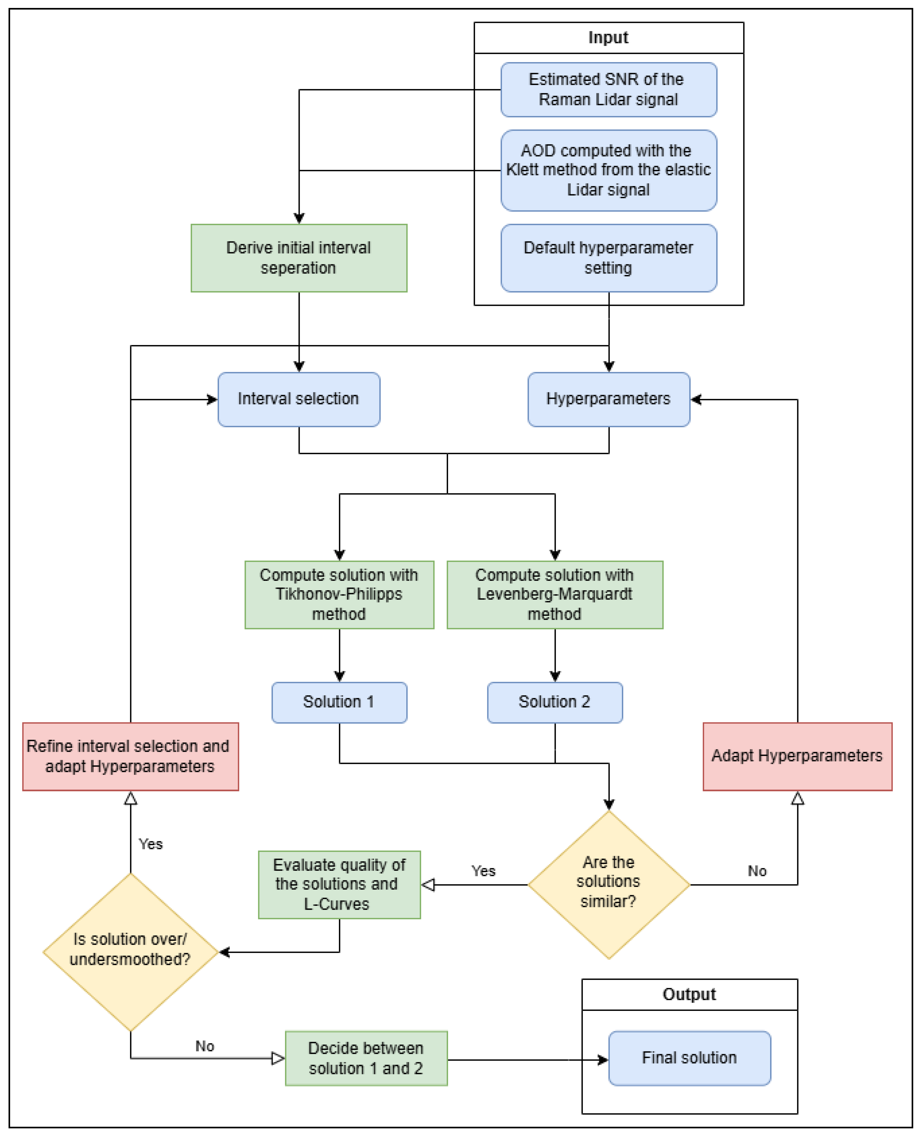
2.1. Basic Algorithm

Any signal P is given as a discrete point set P ¯ = [ P ¯ 1 , , P ¯ n ] . In fact, there is an equidistant grid { R 0 , , R n } with a grid length h from R 0 = H base up to R n = H max , where H base is the height of the base station and H max is the maximum height, for which we calculate the extinction. The discrete points are given by
P ¯ i = R i 1 R i P ( r ) d r h P ( R i )
for i { 1 , , n } . To apply the theory from Appendix A and Appendix B to these data, we need a discretization of y (see Figure 2 as well). Therefore, we approximate y as a piece-wise constant function
y ( R ) i = 1 n y ¯ i ϕ i ( R )
with the base functions { ϕ 1 , , ϕ n } given by
ϕ i : [ R 0 , R n ] R : r ϕ i ( r ) : = 1 if R i 1 < r R i 0 else
similar to the base function from Appendix B. Instead of the true values y ( R i ) , which are not available, we use approximated values y ¯ as coefficients. They are defined as follows (in practice, the term ln ( h ) can be neglected since it is constant and cancels out in (11) anyway):
y ¯ i : = ln P ¯ ( R i ) R i 2 N Mol ( R i ) + ln ( h ) = ln 1 h P ¯ ( R i ) R i 2 N Mol ( R i ) ln P ( R i ) R i 2 N Mol ( R i ) = y ( R i ) .
The task is to differentiate the data vector Y over the interval of interest [ R s , R t ] with 1 < s < t n ; in detail, the vector is
Y = [ y ¯ s , , y ¯ t ] y ¯ s 1 · [ 1 , , 1 ]
in [ R s , R t ] such that R s is a height where now overlap occurs anymore. With respect to R t , we want to mention an a priori criterion for the data quality. The extinction coefficient states how much (percentage) of the light is absorbed or scattered from particles at height R. Thus, this value has to be always positive. Looking into Equation (4), we see that also the derivative (see Equation (5)) has to be positive, even bigger than α λ 0 , Ray ( R ) + α λ Ra , Ray ( R ) . Hence, a monotonically increasing signal function y is expected. For our example, looking at Figure 2(right), we deduce that, for heights R > 4500 m, no more information may be contained in the Raman signal, and we should choose R t < 4500 m.
Then, the solution function x = y in [ R s , R t ] is given as
x ( R ) j = s t x j ϕ j ( R )
where the coefficients X = [ x s , , x t ] solve
A X = Y .
Here, the matrix A is the discretization of the classical integral equation according to Appendix B (see Equation (A19)). We point out that the constant shift y ¯ s 1 in Equation (11) does not change the derivative, but is necessary as described in Equations (A15) and (A18).

2.2. Algorithms for Splitting the Data (SI)

A variable noise level is a problem for regularization. Every theoretically admissible parameter choice rule does depend on the noise level [23]. We deduce that, in general, every parameter choice α for given noisy data fits best to a certain noise level. Hence, if the noise level is not constant, the parameter α cannot be optimal for every part of the solution. Thus, in methods 3 and 4, we consider splitting the data vector Y into smaller pieces (splitting of interval (SI)), differentiating them piece-wise, and sticking the solution together. We separate the interval of interest [ R s , R t ] into part-intervals as follows:
[ R s 1 , R s 2 ] , [ R s 2 , R s 3 ] , , [ R s K 1 , R s K ]
with s = s 1 < s 2 < < s K = t . By splitting the interval, we may compute different regularization parameters for each part-interval. Sticking the solutions together should, hence, lead to an improved result.
Although this turns out to be very promising, especially for high altitudes, we need to decide how to split the interval. At least the following two a priori choices are possible:
  • Based on the noise of the data, choose an interval separation such that every single interval has approximately the same noise level.
  • Based on the cumulative sum of the extinction solution α ¯ Aer = β Aer · L R from Klett’s method, consisting of the backscatter coefficient β Aer and the Lidar ratio (LR), determine an interval separation such that
    j = s i s i + 1 α ¯ ( R j )
    is constant for every i { 1 , , K 1 } . That is, in every part-interval, there may be the same amount of information (extinction).
Furthermore, we will test an a posteriori interval choice method from Pornsawad et al. [16], which introduces the interval length as an additional regularization parameter. We define
I t ˜ , k = [ R t ˜ , R t ˜ + k ]
for k < t t ˜ . The method works as follows:
  • Input: Discrete data Y for the interval [ R s , R t ] of interest (see Equation (11)).
  • Output: Regularized discrete derivative X.
  • Set t ˜ = s .
  • For k { 4 , , ( t t ˜ ) } , compute the regularized derivative X k of Y in I t ˜ , k with a regularization method and the L-curve parameter choice rule. Store the regularization parameter α k and its corresponding curvature c k of the L-curve.
  • Set k * = arg max c k . Store X k * as the final solution over I t ˜ , k * = [ R t ˜ , R t ˜ + k ] .
  • Set t ˜ = t ˜ + k + 1 and restart at (2) until t ˜ t .
The idea is to choose intervals with “good” L-curves. This should ensure that a good regularized solution could have been determined. Note that k 4 in step 2 is necessary, as this is the minimum number of points that we need to calculate the curvature of the L-curve. By choosing a higher value for the lower bound of k, it is possible to enlarge the minimum length of each part-interval.
Additionally, the two parameters k up and k down can be specified. They define the number of discrete points, which we are adding to the part-interval at both ends before calculating the derivative. After computation, we just take the solution from the original part-interval. Thus, we get rid of possible uncertainties occurring at the interval ends. For example, we observed that, at both ends of the part-interval, mathematical oscillations may occur. Furthermore, the solution near the left end of the interval is partly influenced by the shift value.

2.3. Appropriate Shifting of the Data

As mentioned before, the shift of the data Y has an impact on the accuracy of the solution. This is especially of interest when splitting the interval, as we need to shift the data again for every part-interval. Since the data point y ¯ s 1 (default shift) may also be highly influenced by noise, we must find another way to shift the data. The main idea here is to approximate the shift y ¯ s 1 by the solution X = [ x r , , x s 1 ] of the below interval [ R r , R s 1 ] , if it exists. We have
y ¯ s 1 y ( R s 1 ) = y ( R r 1 ) + R r 1 R s 1 d d r y ( r ) d r
= y ( R r 1 ) + R r 1 R s 1 x ( r ) dr
y ¯ r 1 + h k = r s 1 x k .
Assuming that [ x r , , x s 1 ] is a good regularized approximation of X over [ R r , R s 1 ] , the uncertainty of this shift mainly depends on the uncertainty of the data point Y ( R r ) . Since the signal-to-noise ratio (SNR) is getting worse with height, this may have a lower uncertainty than Y ( R s 1 ) . We point out that if there is an uncertainty in the calculation of X, this uncertainty is transported with this shift into the next interval. If no solution of a lower interval is provided, but we are already at altitudes, where the data are very noisy, we consider approximating the shift y ¯ s 1 by any running mean.

2.4. The Levenberg–Marquardt Method with Variable Step Width

The Levenberg–Marquardt method comes with a relaxation parameter γ in the following, considered as the step width. This step width can be chosen arbitrarily for the Levenberg–Marquardt iteration [13,24,25]. Larger step widths allow a faster convergence to the “exact” noisy solution, whereas small choices for γ result in very slow convergence towards the “exact” noisy solution. Observations in test cases lead to the result that there exists a relation between the L-curves of the iterated solutions for different values of γ . Independent of the choice of γ , there exists always just one L-curve, i.e., a set in R 2 on which every pair ( x , K x y ) of every possible iterated solution of the Levenberg–Marquardt method obtained with any step width lies. If the step width now is too small, the progress toward the exact solution is very slow, and it may occur that even large numbers of iterations do not reach the L-corner. If the step width in return is too large, then the L-corner may be “jumped over”. To prevent both, we consider calculating a few iterations with a small step width and then restarting the iteration with a slightly larger step width. This time, we take the last iterated solution as the starting value for the new one. Hence, we are making our way along the L-curve without making very big jumps. It turns out that now the L-corner is much more likely to appear. However, small discontinuities of the L-curve after an increased step width occur sometimes. As this may result in an unstable curvature calculation, we consider interpolating the L-curve piece-wise. As this method uses not just one but different values for the relaxation parameter γ , we call it the variable Levenberg–Marquardt method.

3. Results

3.1. Sensitivity Quantification

Before presenting the proposed methods in different case studies of real Lidar data, we will demonstrate the applicability of the regularized retrieval of the extinction coefficient profile for a synthetic case with a known solution.
Exemplarily, we use the Levenberg–Marquardt method with an a priori interval choice (method 3b). The focus does not depend on the choice of intervals, but rather on the behavior of the method under variational noise. Therefore, a synthetic Lidar profile was generated by solving the inelastic Lidar equation with an assumed extinction profile (solution from Section 3.2 at UT 8:02). This Lidar profile has been disturbed twenty times randomly by a uniform noise, which mimics a realistic noise level. We added this artificial noise to the synthetic Lidar profile. This was performed by an estimation of the maximum uncertainty of the Lidar profile for each height step. This uncertainty profile was then multiplied twenty times with a random number in the range of [−1, 1] for each height step.
In Figure 3, the twenty different input Lidar signals and the average solution (the extinction profile) over all these twenty cases are shown. The original, not smoothed, non-regularized “direct” solution of Equation (5) is presented in cyan, while the regularized solution, obtained with the Levenberg–Marquardt method, is presented in magenta. Both functions of Figure 3(right) are the average of all noisy realizations. A drastic improvement of the precision was found, by which the extinction profile can be retrieved using regularization.
In Figure 4(left), the individual extinction profiles for these 20 Lidar profiles with artificial noise are shown. We observe overall similar profiles that tend to deviate more with height. Figure 4(right) displays the mean and maximum absolute deviation to the original extinction profile averaged by a running mean. The curves clearly show that the deviation grows with altitude, which is natural, since the SNR decreases. Still, all individual solutions appear similar in Figure 4. We conclude that, through regularization, the retrieval of the extinction is possible up to higher altitudes compared with the non-regularized solution.

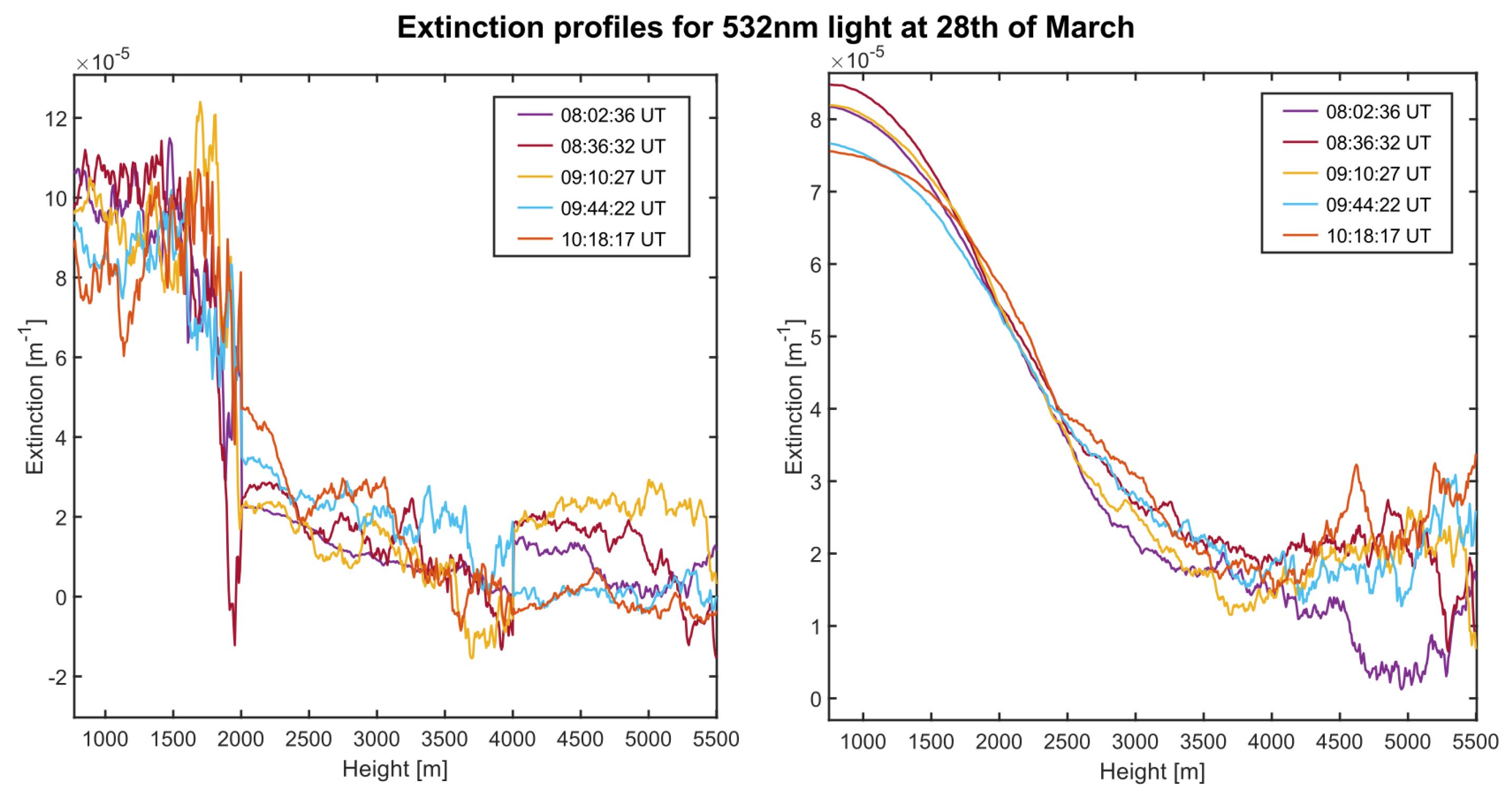
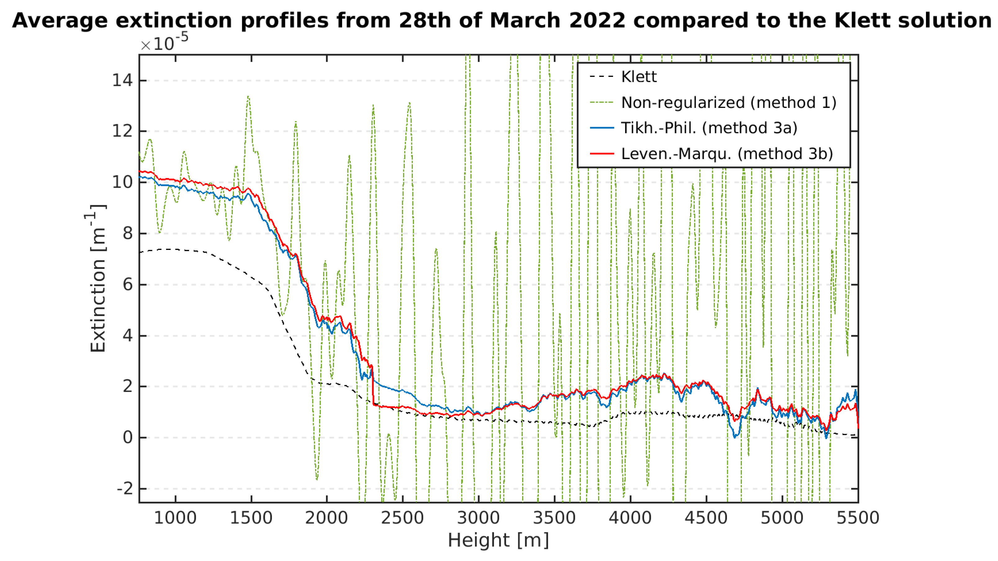
3.2. Analysis of Data from 28 March 2022

In this section, we will apply the regularization techniques to a case of Arctic Haze during daylight. We will derive the extinction profiles for two different time steps and interpret the results in terms of the local wind field.

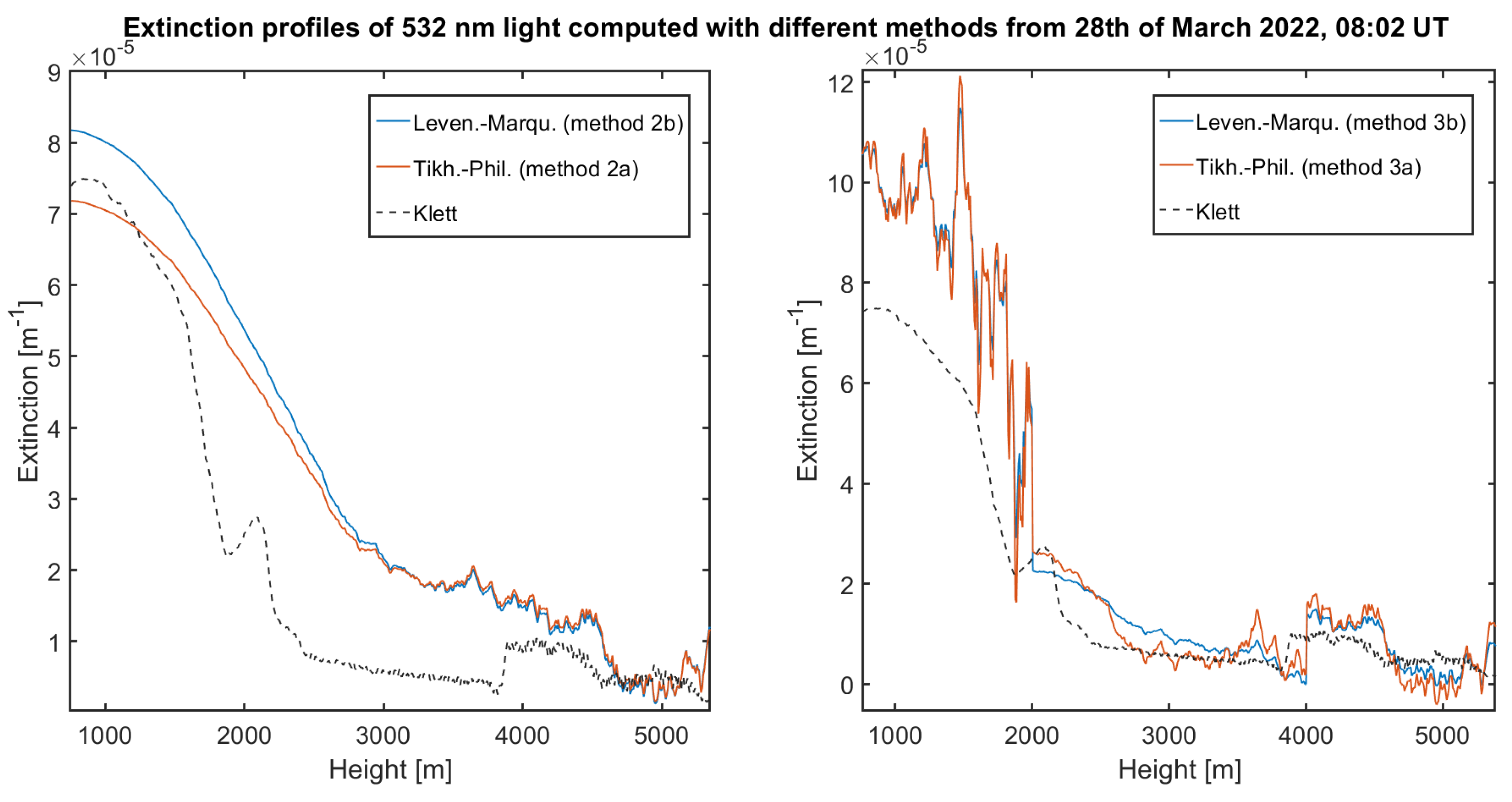
3.2.1. Comparison of the Tikhonov–Phillips and Levenberg–Marquardt Methods

To present an overview of the conditions on this day, we consider the backscatter ratio (BSR) at 532 nm first. The BSR at a given wavelength is defined as
B S R ( R ) : = β Aer ( R ) + β Mol ( R ) β Mol ( R )
and is shown in Figure 5.
The data were obtained via Klett’s method, i.e., without the use of the Raman Lidar signal. The solution with Klett’s method was computed with an arbitrarily predefined constant Lidar ratio of 50 sr for these altitudes. One can easily see an increased backscatter up to an approximately 2 km altitude. The maximum of the backscatter occurs between 08:00 UT and 09:00 UT at a height slightly above 1 km. Above a 2.5 km altitude, the atmosphere is very clear and backscattering mainly occurs on air molecules.
A first step to evaluate the quality of the Raman Lidar signal P 607 can be performed by comparing the critical term Y (Equation (5)) with Klett’s solution. For the analysis of this day, we decided on the analog measured signal (P607analog). A plot of this signal and the corresponding term Y, which we want to differentiate, is shown in Figure 2 for the time step at 08:02 UT. Looking at Y, we assume that its derivative should be positive and nearly constant up to 1500 m. It should decrease afterwards to almost 0 above 2500 m. Beyond this, the derivative should stay constant at 0, except for a small peak at 4500 m. This observation fits approximately the extinction calculated from the Lidar ratio and the backscatter coefficient obtained by Klett’s method Figure A6. Hence, we deduce that the Raman Lidar signal contains enough information for a promising analysis with the method of Ansmann et al. [14]. As the signal-to-noise ratio is relatively good up to 2000 m, we expect that even the non-regularized solution is acceptable at this altitude and should, in mean (averaging over time and height), give the same result as the regularized solution.
In Figure 6(left), the regularized solutions with Tikhonov–Phillips regularization and the variable Levenberg–Marquardt method are shown for the selected time step. The corresponding regularization parameters were determined using the L-curve method (cf. Figure 7). Table A1 and Table A2 in Appendix D list the parameters chosen for this case.
We observe that both algorithms produce nearly the same solution, whereby the solution of the Levenberg–Marquardt method seems to be a little bit smoother. The same result occurs for other time steps (see Figure A7), because the L-curves, which are almost identical for both methods, show good behavior. Therefore, we can assume that a solution was found that fits well to the exact signal.
However, it can be seen that the solutions with methods 2a and 2b are quite over-smoothed at lower altitudes (first half). This was expected since the signal-to-noise ratio decays significantly over the interval. Hence, the regularization parameter fits best to the worst noise level occurring at the end of the interval. Therefore, we consider to split the interval, such that we have an approximately constant SNR in every interval. Looking at the data, the choice of the intervals [ 750 , 2000 ] , [ 2000 , 4000 ] and [ 4000 , 5500 ]  m is reasonable. The solutions with methods 3a and 3b, i.e., with interval splitting, are shown in Figure 6(right).
Now, we observe that the first interval is not as smooth as before. Again, both methods give approximately the same result, while the solution from the Levenberg–Marquardt method seems a little bit smoother. In the third interval, both solutions are almost identical to the solution from the first attempt. Here, the regularization parameters are the largest, with just 10 iterations ( α = 1 10 ) for the Levenberg–Marquardt solution and α = 1.4175 · 10 5 for the Tikhonov regularization. This result can also be observed for other time steps (cf. Figure A7). An analysis of the Raman signal P 387 shows results of similar quality. In Figure A8 (left), the extinction for λ = 355  nm is shown. However, it seems like the solution for the first interval is too noisy. Since the data for those time steps, as well as the L-curves, look quite similar, we can manually adjust the regularization parameter for the first interval. Fixing the number of iterations for the first solution to 40, we obtain smoothed solutions shown in Figure A8(right). Now, we can see a clear correlation between the data from one step to the next. This is a good sign since the aerosol particles in the air change just a little over this period according to the B S R displayed in Figure 5. However, also this small change is observable with the regularized solutions and will be shown in the next subsection.
We were able to show that the regularization methods together with a manually chosen interval separation provide adequate solutions for the extinction coefficient. Calculating an average extinction value over certain time steps and altitudes can then be used to calculate the particle size distribution in an appropriate layer. Nearby, determining the particle size distribution from extinction and backscatter coefficients is again an ill-posed problem and requires regularization for itself (cf. Ritter et al. [26], Dube et al. [27]). Hence, any additional information, like the proposed stable results from the Raman Lidar signal or an additional infrared wavelength (cf. Böckmann et al. [12]), may improve results significantly.

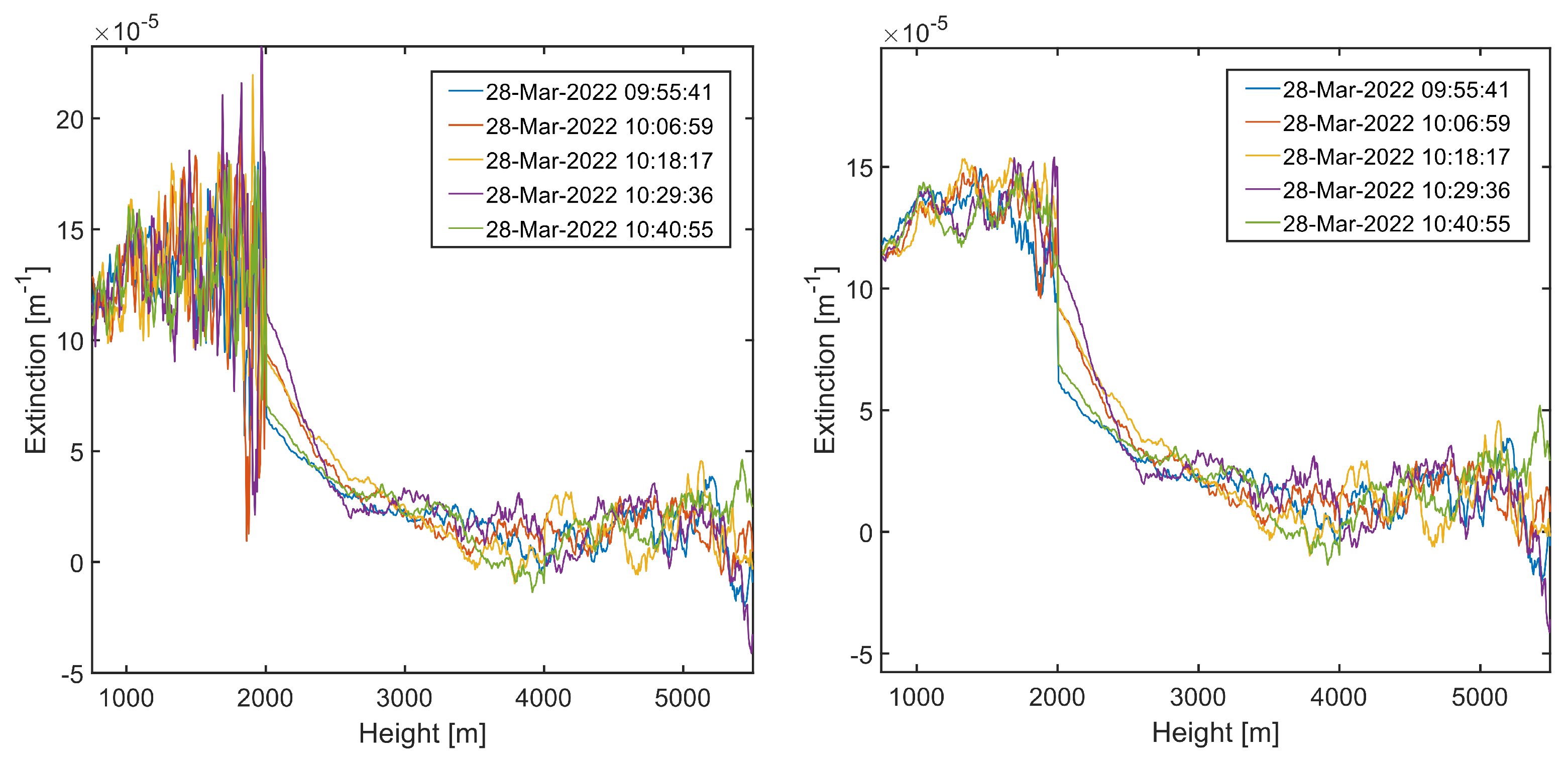
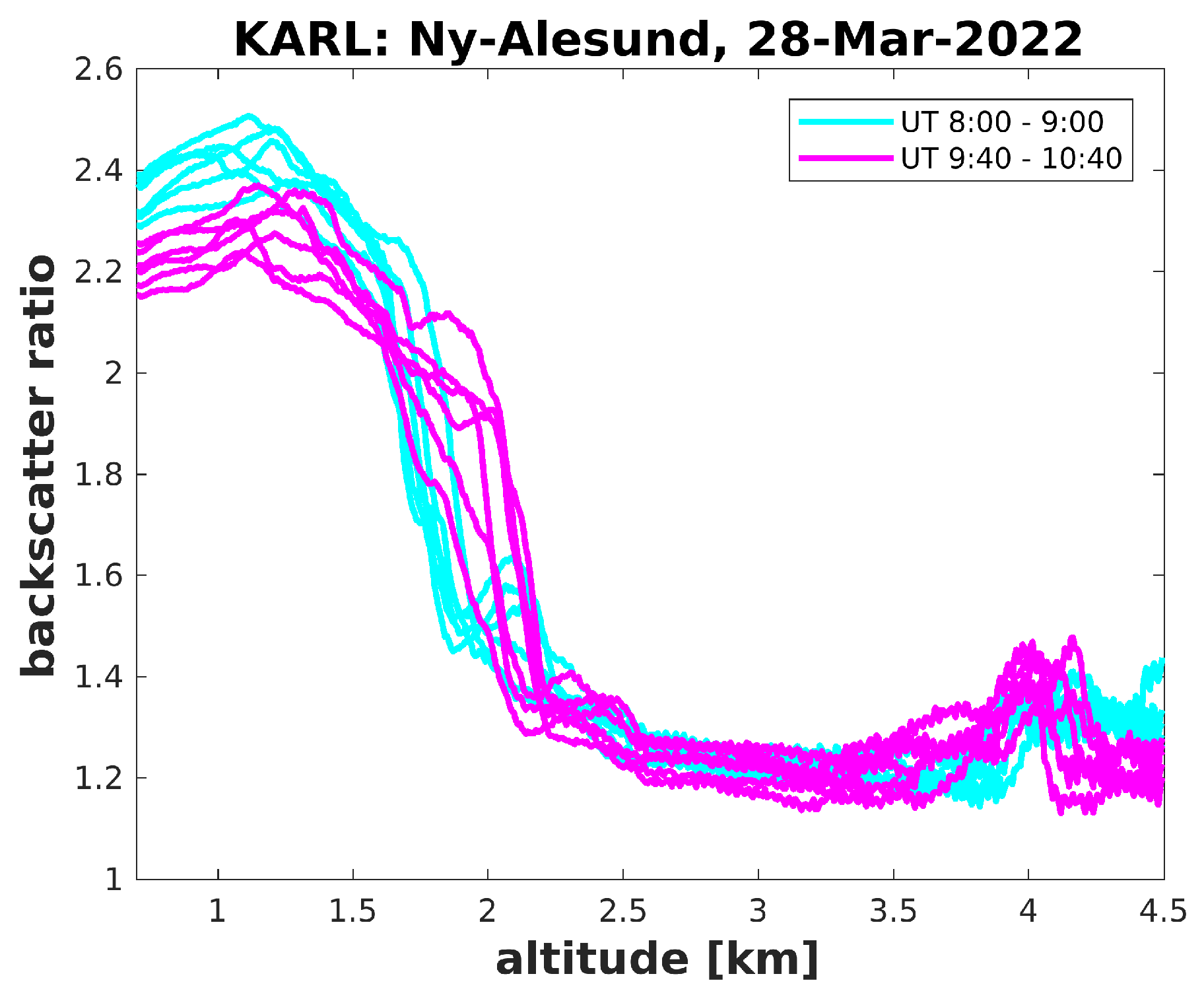
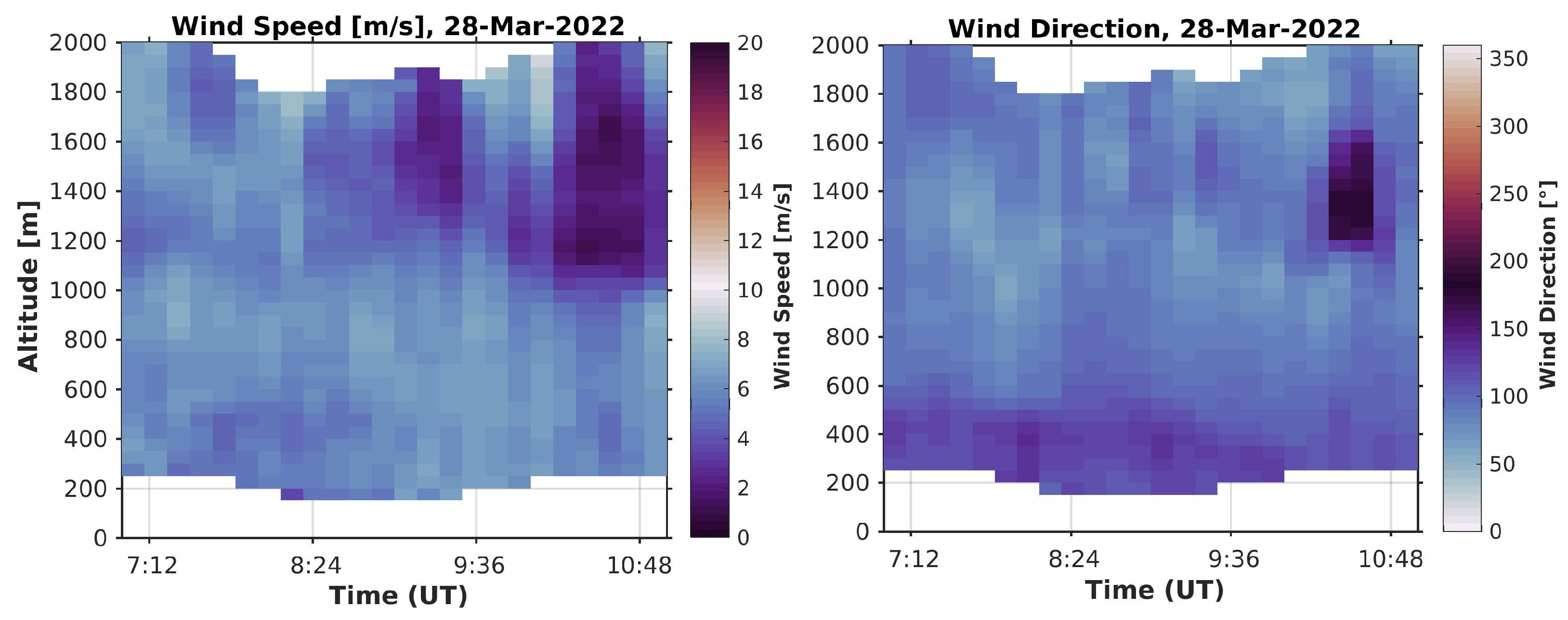
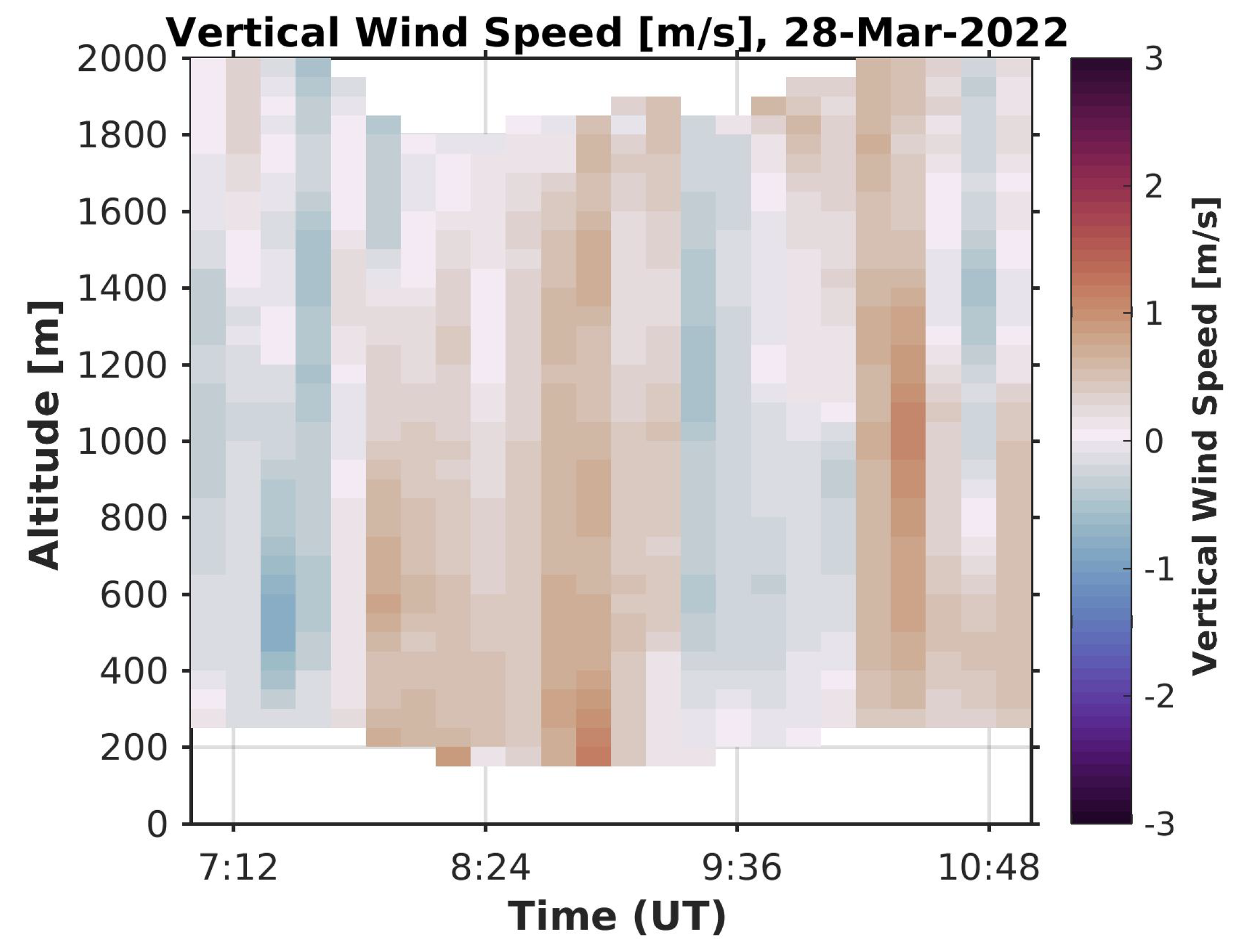
3.2.2. Comparison with a Doppler Wind Lidar

At this point, we want to use the regularized extinction values to analyze any temporal variability of the aerosols. The following comparison with the wind Lidar would not be possible with a classical non-regularized solution of the extinction profile as such solution is dominated by the noise. From the plot of the BSR in Figure 5, we observe the highest concentration of aerosols between 8:00 and 9:00 UT in altitudes below 1500 m. The maximal values of the BSR then clearly reduce until 10:00 UT. However it seems as if the particles were vertically shifted upwards. Now, the task is to explain this behavior of the aerosols. We analyze wind Lidar data from a Leosphere “windcube 200” at the same measurement site as the Raman Lidar to test the hypothesis, whether the decrease in BSR might be an advection phenomenon. More information about the wind Lidar is given in Graßl et al. [28]. Figure 8 presents the horizontal wind speed and the wind direction during that time. In the altitude of maximal backscatter, about 1 km to 1.5 km altitude, a wind speed of about 8 ms−1 from the east is observed. This wind speed might have caused the advection of different air masses, carrying distinct aerosol properties above Ny-Ålesund.
Although the vertical wind speed slows down a bit at 8:00 UT at an altitude of approximately 1000 m, the wind direction remains constant at 10:00 UT. Hence, we have no indication that a completely new air mass is transported towards our observation site. Still, temporal variations of aerosol load in an air mass does occur. To elaborate this, we compare the aerosol extinction coefficient between approximately 8:00 and 9:00 UT and compare this with the extinction between 9:40 and 10:40 UT. This result is presented in Figure 9.
We observe that the extinction value of the latter time period is approximately 2 · 10 5 m 1 smaller than at the earlier time. However, at this latter time, the aerosol layer has a larger vertical extent as the extinction value declines about 200 m higher. Above 2500 m, both extinction values are almost equal. From this result, one can deduce that the aerosols move vertically over time. By computing the cumulative sum ( A O D ) of both solutions, we can compare the total aerosol load in both time periods. The A O D at 2500 m from the first time period is A O D 1 = 0.02509884 , whereas the A O D at the same height from the second time period is A O D 2 = 0.0250964 . This leads to a relative difference of <0.1% and confirms the statement that we are observing the same aerosols. Finally, the vertical wind profile shows that there were indeed mostly updrafts between both times (Figure 10). Hence, the vertical wind from the wind Lidar gives an independent reference for the calculated extinction coefficient. As also the cumulative backscatter (Figure 5) is quite constant for both time intervals, our derived extinction profile can be easily explained by a constant aerosol load, which is simply uplifted by the wind.

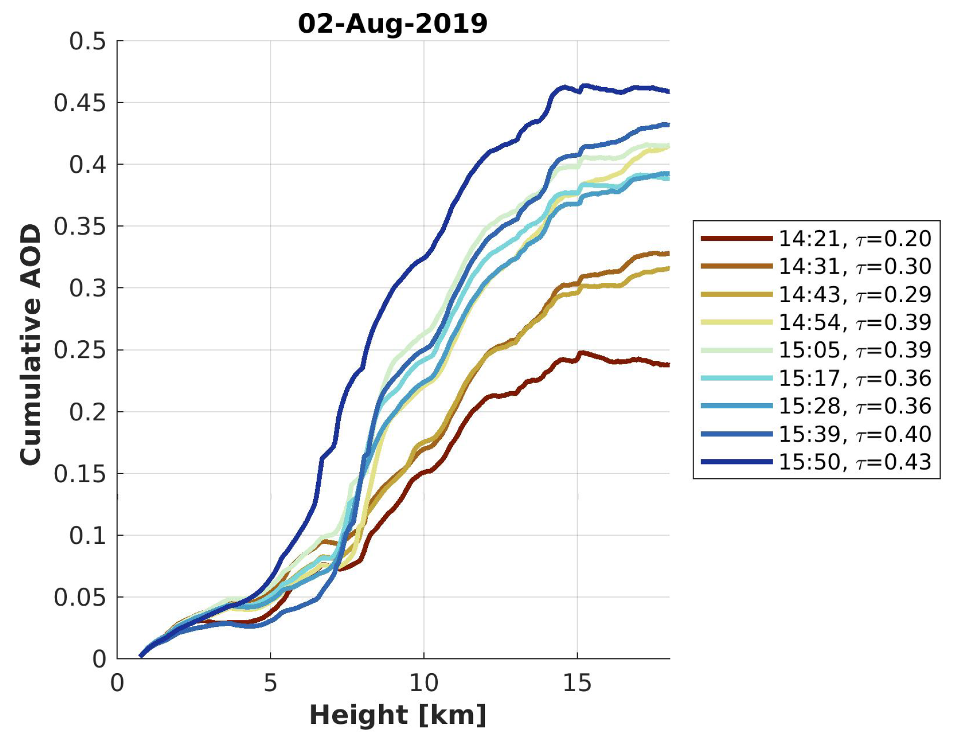
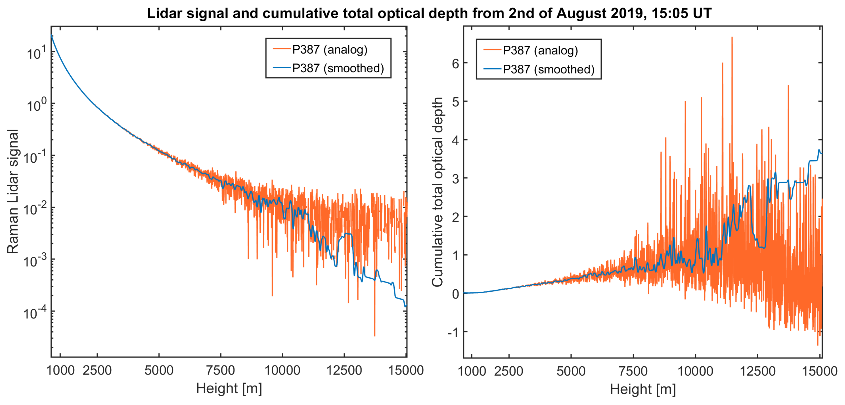
3.3. Analysis of Data from 2 August 2019

In this case study, we investigate aerosols in heights above 5000 m again under daylight conditions. The aim is to compute a stable solution for the cumulative AOD. To compare our results, we will use solutions of the cumulative AOD computed with Klett’s method [29]. Klett’s solution was computed with a constant and arbitrary Lidar ratio of 50 sr (cf. Figure 11). Using the definition of the cumulative AOD, we expect its value to increase stronger the higher the extinction coefficient is. Hence, up to 5 km, only low extinction occurs. Depending on the time step, beyond 5 to 7 km, the cumulative AOD increases significantly faster up to 15 km. Hence, in this interval, we expect more aerosols. Now we will try to obtain similar solutions for the cumulative AOD from the Raman signal. An analysis of the Raman Lidar signal P387analog shows that the term y starts to decrease above 10,000 m. Hence, we will set our interval of interest to [ 750 , 10000 ]  m. To compute results at these high altitudes, it is recommended to use SI (methods 3 and 4). We will compare all different regularized methods with Klett’s solution. Furthermore, it is theoretically possible to compute the cumulative AOD directly from the total cumulative AOD y. Since
y ( R ) = y ( R 0 ) + R 0 R α λ 0 ( r ) + α λ Ra ( r ) d r
we can derive the cumulative AOD of λ = 355  nm light directly. Therefore, we use the Ångström exponent equation (Equation (3)) with a sufficient choice of 1.2 of the Ångström exponent [30]. Furthermore, we use the Rayleigh extinction of the 355 nm and 387 nm light. They can be computed directly from air density and temperature. Putting it all together, we decompose y to
A O D 355 nm ( R ) = y y ( R 0 ) R 0 R α λ 0 , Ray ( r ) + α λ Ra , Ray ( r ) d r 1 + 387 355 1.2 .
A positive result would be that the regularized solution behaves like the solution from Klett’s method and at the same time like a good interpolation of the AOD derived in Equation (22).
We used the analog measured signal P387analog as well as a smoothed signal. (The smoothing was performed by applying a running mean on the range and density corrected Lidar signal.) Up to about a 11 km altitude, this smoothed signal approximates P387analog, as can be seen in Figure 12. Above 11 km, the smoothed and the original signal diverge and are dominated by noise.
All three regularized methods were applied to the analog signal P387analog. Furthermore, one solution with the smoothed signal was calculated over the whole interval [750, 10,000 m] (method 2b). The results can be seen in Figure 13 for the time step 15:17 UT. The regularization parameters for the methods with multiple intervals can be read up in Appendix D in Table A3, Table A4 and Table A5. Table A3 and Table A4 correspond to methods 4a and 4b, the a posteriori interval splitting methods. We observe that the regularization parameter is increasing in both scenarios (recall that the regularization parameter for the Levenberg–Marquardt method is given as 1/(number of iterations)). This can be explained by the fact that the signal-to-noise ratio is constantly decreasing with height, forcing a stronger regularization. In contrast to the other methods, the regularization parameter does not increase with height. This is not obscure in that case since the third interval contains a peak of the extinction profile. To retrieve those high extinction values, a larger number of iterations (smaller regularization parameter) was necessary, which could also be determined by the algorithm.
Generally, it can be seen from Figure 13 that the cumulated AOD up to a 10 km altitude in all different methods only differs by about 30%, and the uncertainty of the AOD retrieval is about 0.011. As expected, the solutions calculated for the whole interval (method 2b) tend to be over-smoothed. For this reason, the steep increase in extinction starting at about a 7500 m altitude is underestimated in some solutions. The Tikhonov–Phillips method with a posteriori SI (method 4a) does this as well. Compared with the AOD from Klett’s method, the regularized methods produce higher AOD profiles. This is not necessarily an error, but instead indicates that the Lidar ratio in Klett’s method was slightly underestimated. Comparing the qualities of the solution, we observe that the variable Levenberg–Marquardt method with a posteriori SI (method 4b) and with SI according to Klett’s AOD (method 3b) fit best to the AOD from Klett’s method. Both methods can determine a critical height between 7000 m and 8000 m, where the AOD starts to increase faster. Especially, method 3b (green graph in Figure 13) visually serves best as an approximation of the AOD, which was directly computed from the signal P387analog (gray graph). The following four major conclusions can be drawn from this case study:
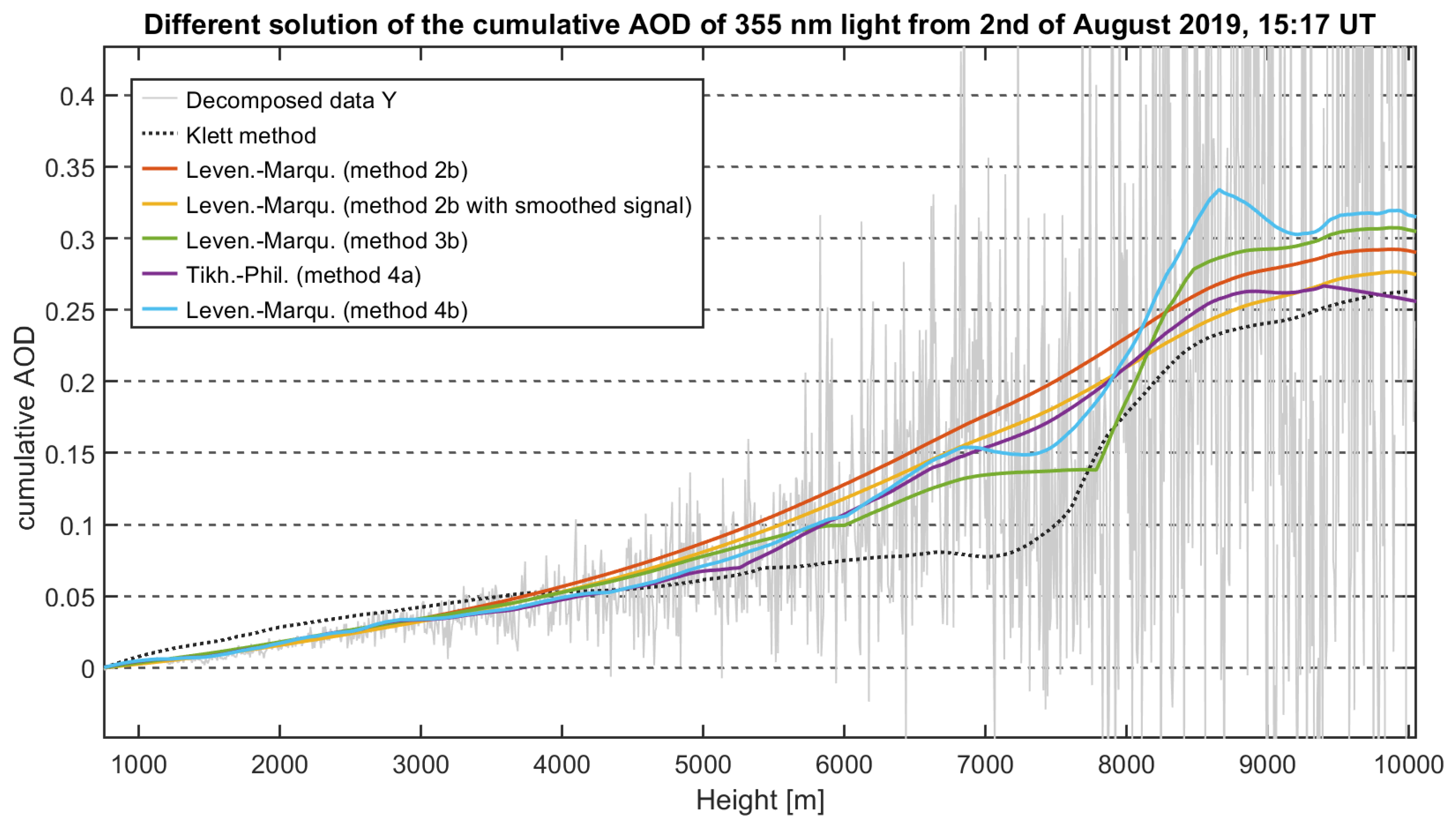
  • To prevent over-smoothing, it is recommended to use SI. This separation of the intervals needs attention as too narrow intervals (too little information content) may lead to non-physical results. In Figure 13, the solutions with a posteriori SI show few altitudes, in which the cumulative AOD shows a decrease with altitude, corresponding to a negative extinction. This can happen if the information content in the interval is too small compared with the noise. Regularized solutions (of the extinction) are not restricted to positive semi-definite values.
  • Although the Levenberg–Marquardt and Tikhonov–Phillips regularization might produce a similar result over a fixed interval, the solution can differ if the a posteriori SI is used. In this case study, only the Levenberg–Marquardt method was able to give meaningful results in combination with the a posteriori SI. Hence, it is in general good to have both regularization techniques in hand.
  • An interval split according to Klett’s solution is promising and produces, in this case, the best-regularized solution.
  • A pre-smoothing of the Lidar data does not clearly improve the range for a valid retrieval of the extinction coefficient and is therefore not necessary.

3.4. Analysis of Data from 18 October 2021

Finally, we present a case with strong extinction (a cloud) under dark conditions. Additionally, this example shows an increased range, in which a valid extinction coefficient can be retrieved by regularization. The measurements are again from Ny-Ålesund on 18 October 2021. Inspection of the Raman Lidar profile (Figure 14) indicates a significant extinction in heights between 2100 m and 2600 m. Above that altitude, noise in the Lidar data is observable. Since we are in relatively low altitudes and measurements were taken by night (no background light), the traditional Ansmann algorithm is already capable of producing a plausible solution for the significant extinction between 2100 m and 2600 m (cf. Figure 15d). We want to test in this case study if the regularized solutions verify the Ansmann method up to 2600 m and give meaningful full results for the extinction profile above.
We use this example to demonstrate the importance of selecting appropriate intervals and show how it can be done. In the previous case study, we already used an a prior SI method, which was based on Klett’s solution. In this example, we will develop a solution by choosing a step-by-step finer part interval. We have chosen the variable Levenberg–Marquardt regularization (method 3b) for computing the piece-wise solutions. First, in Figure 15a, only one height interval (from 700 m up to 6 km) for the retrieval of the extinction coefficient has been considered. An increased extinction is evident slightly above a 2 km altitude. Hence, we subdivided the intervals from 700 m to 1900 m and from 1900 m to 2800 m and above (red lines in Figure 15a). In this way, we obtained the extinction profile of Figure 15b. In this plot, two distinct layers, which are now vertically thinner but show higher extinction coefficients, become apparent. Hence, we redefined the intervals and set the interval borders at 2100 m and 2600 m (red lines in Figure 15b) to obtain the result of Figure 15c. Here, the existence of the two separate layers is confirmed, but a non-physical behavior, just above 2600 m where the extinction becomes negative, is obtained. Therefore, we further subdivided the intervals, as indicated in the plot, and obtained the final solution in Figure 15d. For comparison, also the traditional Ansmann solution (in black) is given. One can clearly see that the extinction of the two cloud layers agrees quite well. Our interpretation is that, in “easy situations”, the simple unregularized solution already gives a good approximation. However, the new regularized solution can produce much more reliable extinction values in the cloud-free altitudes, as can be seen from the lack of odd oscillations above a 2.6 km altitude. Hence, the effective range, in which a valid extinction coefficient can be retrieved, is increased.
In this study, a final strategy for an automated finding of appropriate intervals, in which a regularized extinction is calculated, cannot be given. However, we note that the cumulative AOD (e.g., from the onset of the full overlap up to that altitude in which the Lidar signal becomes too noisy) hardly depends on the choice of these intervals. This is demonstrated in Figure 16. Here, the four different solutions of Figure 15a–d are plotted, which are clearly very similar. Hence, a different interval selection does influence how much extinction (and AOD) is in each interval, but the sum of all AOD values of the intervals is hardly affected by their number. This could be achieved by the use of an adapted shift strategy that relies on the solutions of the lower intervals (cf. Section 2.3).

4. Discussion

In this section, we briefly discuss the usefulness of our approach for real data.

4.1. Discussion of Case Studies

Figure 6(right) and Figure 17 present the extinction profile from 28 March 2022 computed with methods 3a and 3b. It can be seen from Figure 17 that the unregularized “Ansmann solution” (green line, method 1) becomes completely useless beyond a 2 km altitude. The Tikhonov–Phillips and Levenberg–Marquardt solutions (red and blue lines, respectively) are very similar to each other. In Figure 6(right), both methods show an artificial jump in the extinction profile at a 4 km altitude. This is probably due to an imperfect interval selection in this range, as we were at this point mainly interested in the extinction in the lower troposphere and the interval selection focused on a constant SNR in each of the three intervals. The SNR for the 607 nm channel is presented in Figure 18. It can be seen that we have an SNR of about 100 at slightly above a 2 km altitude, while at a 4.5 km altitude, the SNR drops to approximately 50. If using another SI over the part-intervals [ 750 , 2300 ] m and [ 2300 , 5500 ] m, the artificial jump disappears (see Figure 17) by, for example, using an adapted SI with a focus also on the upper range; regularization allows for retrieving a valid extinction coefficient in an increased altitude range too. Finally, we conclude that, for the traditional unregularized solution of Ansmann, a S N R > 100 is mandatory, while, even with suboptimal interval settings (disregarding the jump), our new approaches allow a reliable retrieval of the extinction down to an SNR value of about 50.
A similar improvement in solutions could also be verified in the other case studies. The example from 18 October 2021 (Section 3.4) showed that the new methods could identify a clear sky beyond 2600 m, whereas the traditional method produces noisy results (see Figure 15).

4.2. Discussion of Method Adaptions

Within this study, we presented two regularization methods together with the L-curve parameter choice rule. However, the methods come together with a fairly large variety of different options and hyperparameters. Every new adaption that we introduced (for example, splitting the interval, introducing various shift strategies, or enlarging the interval borders with k up and k down ) in Section 2 improves the algorithm for our setting. On the other hand, it makes the program more complex and difficult to configure. However, we made sure that every new adaption addresses a specific weakness of the base algorithm. Most of the hyperparameters can be set in the same way for different case studies. This paper aims to present the new methods and summarizes various adaptions. The next step would be to further automatize the program, such that it can be used without having to understand every detail of the algorithms. A first step was already performed by Pornsawad et al. [16] with the automated choice of part intervals. Using this method, we were able to compute good mean extinction profiles in our first case study (Section 3.2). However, we observed that this approach does not always lead to meaningful results. Hence, various a priori SI methods were introduced. So far, in each case study, there was at least one strategy that resulted in an improvement of the classical Ansmann solution.

4.3. Utilizing Klett’s Solution to Derive an A Priori SI

At this point, we want to highlight the interval separation strategy based on Klett’s solution. In Section 3.3, this method, together with the variable Levenberg–Marquardt methods, produced the best solution. In the future, one could think of a combined algorithm that may also improve Klett’s solution. Heuristically, it would work like the following:
  • Compute a regularized Ansmann solution of the extinction based on SI with Klett’s solution.
  • Use the regularized extinction profile to update the Lidar ratio assumption for Klett’s algorithm. Compute a possible improved Klett’s solution for the backscatter and extinction coefficients with the updated Lidar ratio.
  • Repeat the above steps until the regularized extinction from Ansmann’s algorithm and the extinction from Klett’s algorithm are arbitrarily equal.
Even if we do not use Klett’s solution for an interval separation, we could use the new stable regularized extinction to update the Lidar ratio and so improve Klett’s solution.

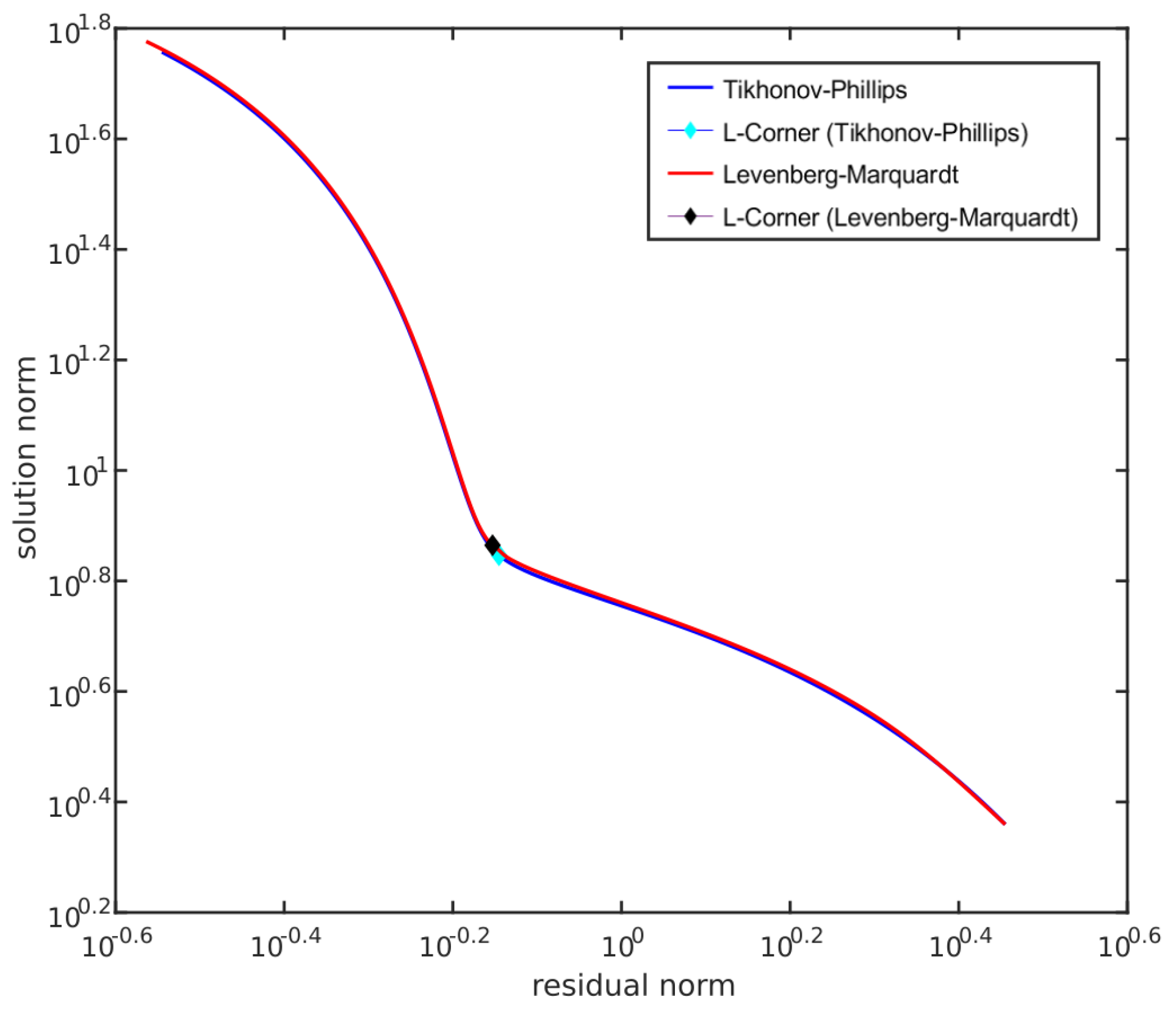
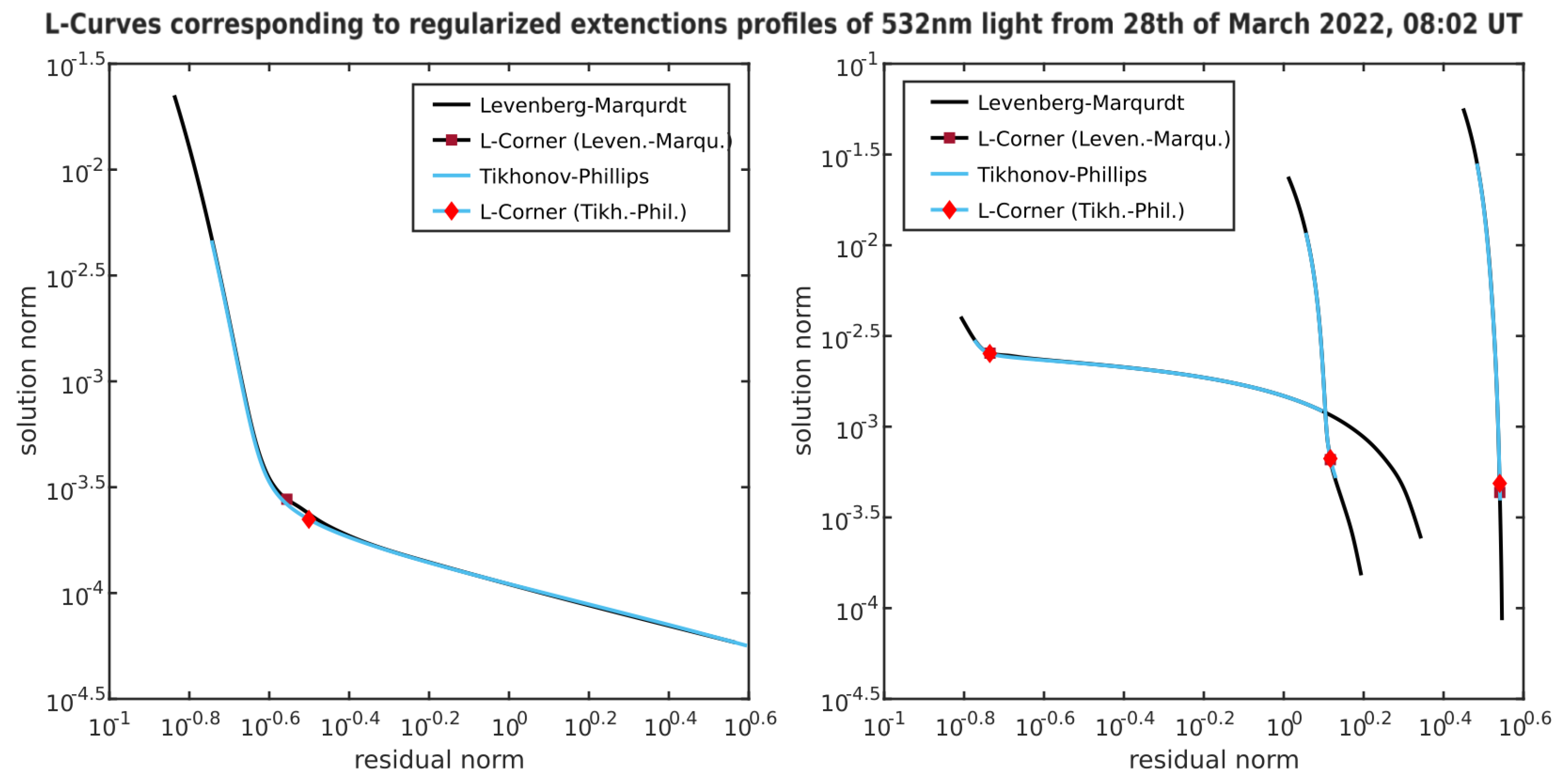
4.4. Discussion of Parameter Choice by L-Curve

Finally, we want to discuss the regularization methods that were used. Both, the Tikhonov–Phillips and the Levenberg–Marquardt methods seemed to be sufficient and promising choices for this task. As we can see, especially in Section 3.2, they often lead to almost identical solutions over the same intervals. However, as soon as we use advanced interval separation (e.g., method 4), the solution may differ. Hence, it is recommended to always have both in your hands.
Using the heuristic parameter choice rule from Hansen [31], which was already used by Pornsawad et al. [16], it was in many cases possible to determine a good regularization parameter. It worked best in cases, where the interval was large or the SNR was sufficiently high. Especially in lower altitudes or over large intervals, a clear L-curve could be observed. Although this L-corner did not always indicate the best solution, it is located often near the best regularization parameter. Introducing the variable Levenberg–Marquardt method (Section 2.4) significantly improved the L-curve quality for the Levenberg–Marquardt method.

5. Conclusions

In this study, we presented the retrieval of the extinction coefficients from Raman Lidar data using different regularization techniques. We considered both solutions of synthetic Lidar data and three different measurement cases from the Arctic, which provides a demanding test environment due to the lack of darkness for more than 6 months and generally low to moderate extinction values.
We applied and tested regularization methods, namely, adaptions of the Tikhonov–Phillips and Levenberg–Marquardt methods. Our main conclusions can be summarized like this:
  • The retrieval of the extinction from Raman Lidar data is ill-posed. The main difficulty occurs at the determination of the derivative of the Lidar signal with respect to the altitude. Hence, regularization provides an adequate tool to handle this class of problems.
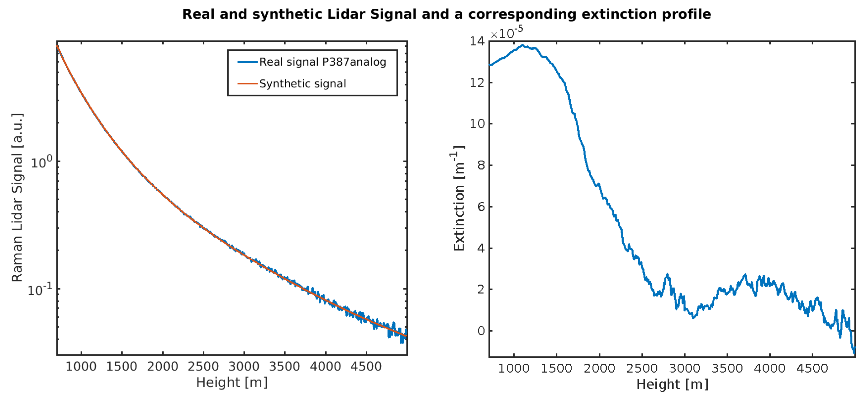
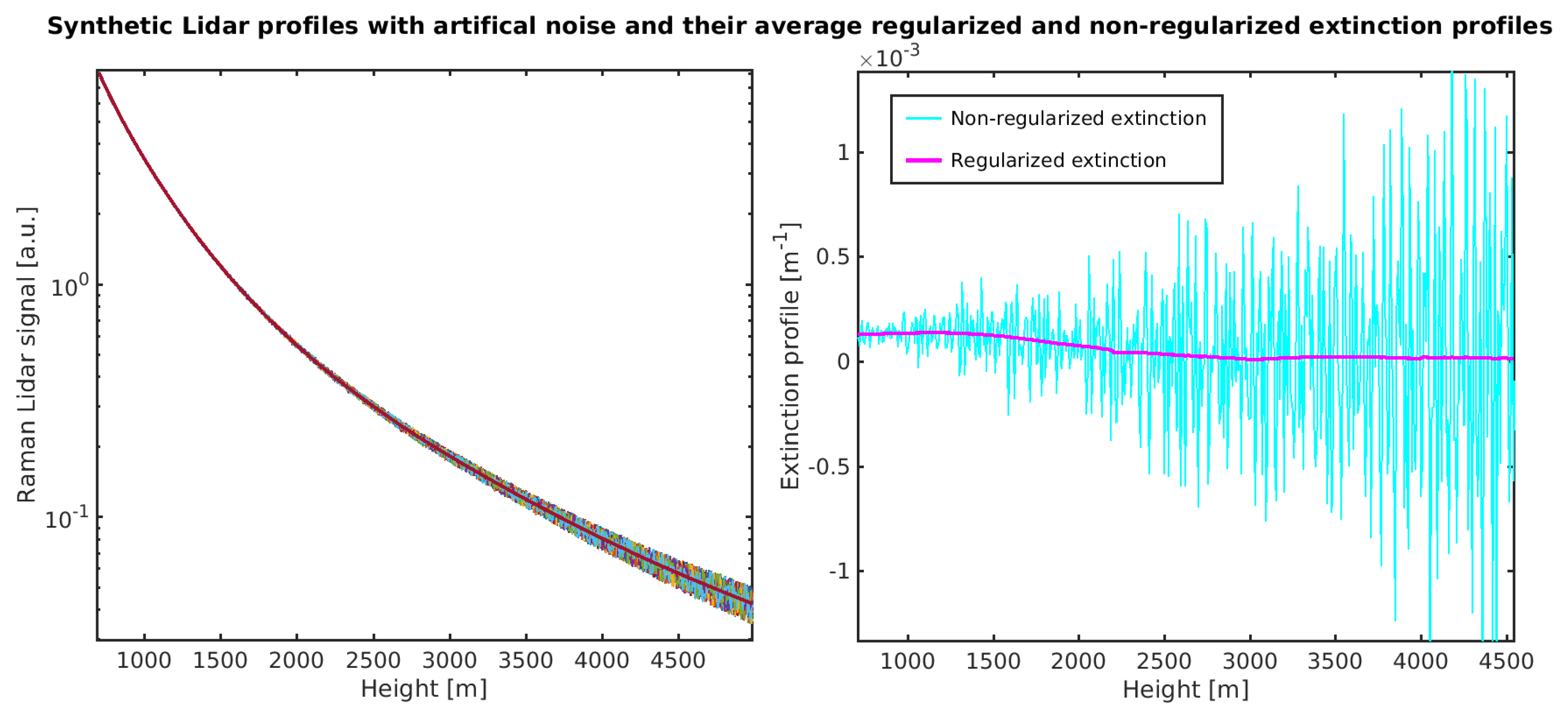
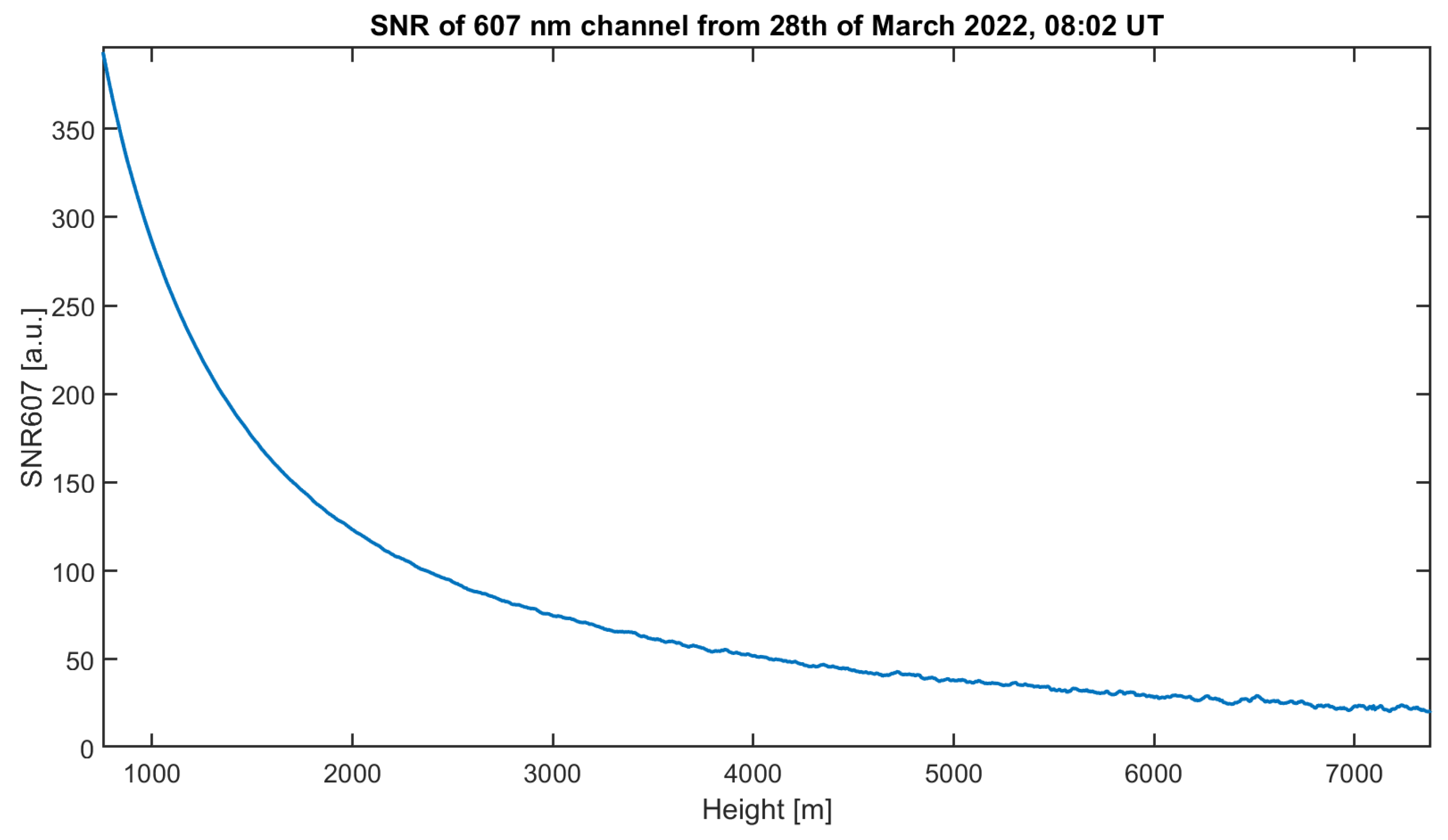
  • In principle, all presented methods work. The retrieval of a trustful extinction coefficient is possible into altitudes, which are clearly higher compared with the traditional non-regularized solution. As a rule of thumb, only half of the signal-to-noise ratio is necessary for our approaches. If the SNR of the Lidar data is very good, only a very small regularization parameter will be found, and the regularized and non-regularized solutions are basically identical.
  • The regularized solution depends on several hyperparameters, which need some attention to obtain best results. Two important ones are the regularization parameter and the interval separation for finding a solution. As the regularization parameter depends on the noise level and seems to be adjusted to the part of a signal with the worst quality (the upper end of each interval), very large intervals present a solution, which is too smooth. Contrarily, in very narrow intervals, it may be difficult to find an optimal regularization parameter, as the corresponding L-curve was oddly shaped.
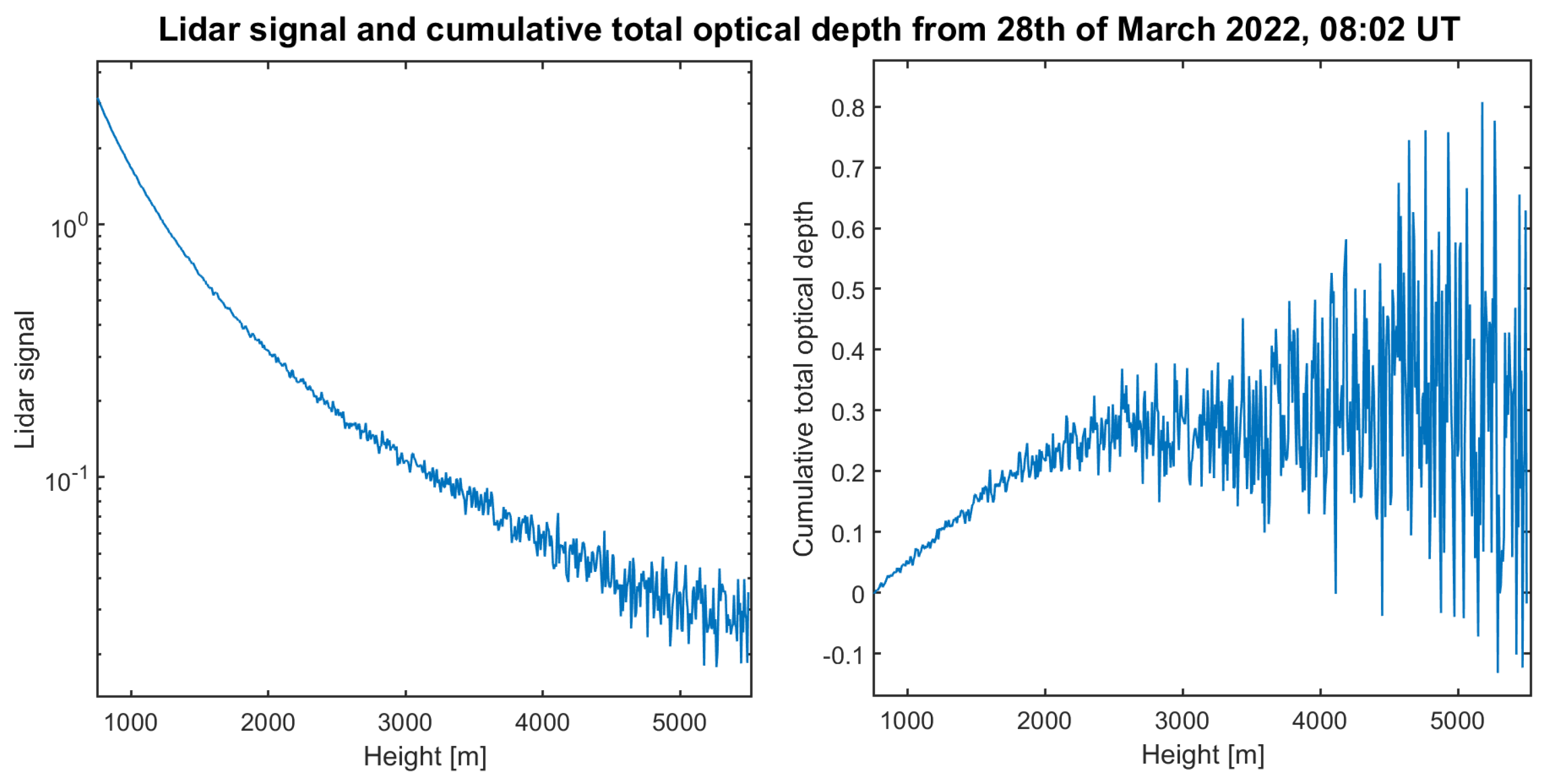
  • Clearly, the cumulative AOD over an extended interval is a quality that is much easier to obtain. In theory, it can be obtained directly by smoothing the Lidar signal (without the need of a derivative). However, the cumulative AOD can also be computed by the regularized solutions, as it is the integral (cumulative sum) of the extinction profile. This is another good approach that comes without any smoothing.
Our main findings concerning the advantages, disadvantages, and peculiarities of the applied methods are summarized in Table 1. Further, we provide a flowchart on the principal concept in Appendix D in Figure A4.

6. Outlook

  • In future work, one should work on an automated choice of the multiple parameters that can be chosen in the presented methods. This could make the algorithms more accessible to other researchers, since these regularization techniques are not only applicable for determination of Arctic extinction coefficient profiles from Raman Lidar but also at other places. In Figure 17 and Figure 18, a relation between the SNR of the Lidar data and the expected accuracy of the extinction profile is given, which should be valid for other sites as well.
  • Another aspect that one might consider in future work is the application of a multiple parameter choice rules. When using the L-curve method, we rely on a correlation between the solution norm and the data error. However, this correlation is sometimes not ideal. Especially for very smooth solutions, the solution norm tends to increase very late, which leads to a smaller regularization parameter at the L-corner. Hence, the solution might be too noisy (Hansen [32], Chapter 8.1). In this case, Hansen [32] recommends using a combination of multiple parameter choice rules. He encountered that using both the L-curve method and a generalized cross-validation (GCV) gives in many cases at least one of two good results. According to (Hansen [32], Chapter 7), the L-curve method is more stable, while the GCV, if it works, tends to give a more accurate regularization parameter. Considering the GCV method, especially if the solution from the L-curve parameter choice rule seems too noisy, is something worth studying in future work. More about GCV can be read in Wahba [33].
  • Non-heuristic parameter choice rules, like the principle of Morzorov, are not suitable for our studies due to the uncertainty about the noise level in our signal. When using the Levenberg–Marquardt and Tikhonov–Phillips regularization during this paper, we came to another interesting assumption. No matter which regularized solution was chosen, it always seems like it fits perfectly to a certain constant noise level. Since the noise level of the provided signal is increasing with height, this means that, especially over large intervals, a regularized solution can only fit well to a certain part of the interval. This also explains why separating the intervals mostly results in better solutions.
  • Our assumption can be underlined at least for the Tikhonov–Phillips method. As shown in Kaipio and Somersalo [34], the Tikhonov–Phillips regularization is equivalent to a Bayesian Inversion method, which models the true signal as well as the noise as a Gaussian distributed random variable with zero mean and a constant variance. Another idea for future work could be to apply other Bayesian models in Ansmann’s algorithm instead of the Tikhonov–Phillips methods. One could choose different models for the noise distribution that may fit better to the given signals. A suitable family of models could be the family of Lévy- α -processes [35], which could be capable of modeling an increasing noise level of the signal. Recent work from Suuronen et al. [35] showed the practical usability of those processes as prior assumptions.

Author Contributions

Conceptualization, R.M.H., C.B. and C.R.; methodology, R.M.H.; software, R.M.H.; validation, C.B. and C.R.; formal analysis, R.M.H. and C.B.; data curation, C.R. and S.G; writing—original draft preparation, R.M.H., C.B. and C.R.; writing—review and editing, R.M.H., C.R., C.B. and S.G.; visualization, R.M.H. and S.G.; supervision, C.B. and C.R. All authors have read and agreed to the published version of the manuscript.

Funding

This research received no external funding.

Data Availability Statement

The original contributions presented in this study are included in the article. Further inquiries can be directed to the corresponding author.

Acknowledgments

We thank the station crew at the AWIPEV station for the Lidar measurements and especially Wilfried Ruhe and Ingo Beninga for their great maintenance work at the station. We further thank Pornsarp Pornsawad for providing us a software package that was helpful to compare and develop our programs.

Conflicts of Interest

The authors declare no conflicts of interest.

Abbreviations

The following abbreviations are used in this manuscript:
AODaerosol optical depth
BSRbackscatter ratio
SSAsingle scattering albedo
SIsplitting of interval
SNRsignal-to-noise ratio

Appendix A. Mathematical Preliminaries

Let K : X Y be a linear bounded and compact operator between two Hilbert spaces (e.g., adapted function spaces) X and Y . For given data y Y ,
K x = y
is called an operator equation. In the context of this paper, K plays the role of the simple integral operator. That means y = K x is an antiderivative of x, and in return, x is the derivative of y. Then, y is the crucial term ln N Mol ( R ) S Ra ( R ) and x its derivative d d R ln N Mol ( R ) S Ra ( R ) . In order to determine x, we face two problems: The data y are not provided exactly, since they depend on the range corrected Lidar signal S Ra . In fact, we have only access to noisy data y δ . Second, solving the operator Equation (A1) is ill-posed, meaning that a small deviation in the noisy data y δ might lead to a totally different derivative x. In the following, we describe several regularization techniques that allow us to reconstruct a solution of Equation (A1) just given the noisy data y δ .
Assuming that there exists a solution x δ of Equation (A1) for noisy data y δ , which is not necessarily unique, we want to choose the solution x with minimal norm, i.e., the best-approximate solution x δ + , which is now unique and given by
x δ + : = K + y δ = n = 1 u n , y δ σ n v n .
K + is the Moore–Penrose generalized inverse of the operator K, δ is the noise level of the given data, and ( σ n ; v n , u n ) is the singular system of the compact operator K. The singular values σ n converge to zero
lim n σ n = 0 .
With this representation, it is fairly easy to see why such infinite-dimensional problems are ill-posed. A tiny noise δ in the nth coefficient is multiplied by 1 σ n . Since 1 σ n as n , the higher coefficients has to be determined very precisely for obtaining a stable result. The following question arises: how do we adjust the operator K + to obtain a stable but in the same way sufficiently accurate best-approximate solution x δ + ? We provide an answer in the next paragraph.
Let M , N R be closed subsets and X and Y be adapted function spaces on M and N , respectively. We now regard a particular linear bounded and compact operator K, namely, a Fredholm integral equation of the first kind, as follows:
y ( s ) = ( K x ) ( s ) = M k ( s , t ) x ( t ) d t
where k : N × M R is a functional and is called the integral kernel.
Our main problem is the stably numerical calculation of the derivative x of function y using Equation (A4). The derivative inside Equation (4) can easily be rewritten into such Fredholm integral equation of the first kind as follows:
K : L 2 ( [ a , b ] , R ) L 2 ( [ a , b ] , R ) : x y ( s ) = ( K x ) ( s ) = a b k ( s , t ) x ( t ) d t
with kernel
k : [ a , b ] × [ a , b ] R : k ( s , t ) 1 a t s b 0 a s > t b ,
For more details, see below.
The idea now is to replace the term 1 / σ n in Equation (A2) using a parameter-dependent filter function F α : ( 0 , K 2 ] R + such that F α is bounded away from 0. Then, the family of operators R α
x δ , α + = R α y δ : = n = 1 F α ( σ n 2 ) σ n u n , y δ v n
eventually could serve as a stable approximation of K + . Well-known filter regularization methods are, e.g., Tikhonov–Phillips regularization and Levenberg–Marquardt regularization. The unique “argmin” of the well-known Tikhonov functional J α
x δ , α + : = argmin x D ( K ) J α = argmin x D ( K ) K x y δ 2 + α x 2
can be computed via the solution of the well-known normal equation [36,37].
However, x δ , α + may also be represented as a filter method as follows:
x δ , α + = R α y δ = n = 1 F α ( σ n 2 ) σ n u n , y δ v n = n = 1 1 σ n 2 + α σ n u n , y δ v n
with α > 0 R + . Now 1 σ n + α if n . It converges to 1 α . The Levenberg–Marquardt regularization is
x δ , α + = R α y δ = n = 1 γ k = 1 1 / α ( 1 + γ σ n 2 ) k σ n u n , y δ v n
with α { 1 , 1 2 , 1 3 , } and γ R + . The index k counts the number of iteration steps and serves as regularization parameter α = 1 / k . The parameter γ is a relaxation parameter, which we explain in the next section in more detail. For the classical Levenberg–Marquardt method, this relaxation parameter is chosen to be constant. However, we investigated that the choice of a variable relaxation parameter can help to find the optimal solution. It allows for computing sequences of solutions that work very well together with the L-curve parameter choice rule. This so-called variable Levenberg–Marquardt method is further explained in Section 2.4. It is equivalent to the classical Levenberg–Marquardt methods with restarts.
Next, we need a parameter choice rule to select a suitable regularization parameter α . In general, it depends on the noise level δ (a priori rule) and, additionally, on the given noisy data y δ (a posteriori rule). There exist a range of different noise-dependent parameter choice rules, like the discrepancy principle of Morozov [37]. However, they often do require a certain accuracy of the noise level δ . If the noise is predicted to be too high, the regularization parameter α will be chosen to be too large, and hence, the approximation error x + x α becomes too big. On the other hand, if the noise is underestimated, the data error x α x δ , α is too high [37].
Therefore, the use of the so-called heuristic parameter choice rules is more convenient for cases in which the noise level δ cannot be predicted accurately enough. It is worth mentioning that such heuristic rules do not strongly fit into the mathematical theory but often works fine in applications. In the following, we briefly present the L-curve parameter choice rule according to Hansen [32]. Therefore, it is necessary to compute the regularized solutions x δ , α for multiple values α and one chooses the “best” solution, which is explained in the next paragraph. However, it is important to choose a wide range ( 0 , α max ] of possible parameters α to ensure that a good parameter α is inside the range.
Given a set of calculated regularized solutions { x α 1 , , x α i , , x α m } , we derive the L-curve by plotting the solution norms x α i against the residual norm K x α i y δ , i = 1 , , m in a log–log scale. The corresponding curve represents how both norms correlate. In parts where the curve is flat, the residual norm decreases faster than the solution norm increases. If the curve is steeper, the solution norm grows faster, and then the residual norm decreases. In many applications, one observes that the curve is relatively flat for large regularization parameters and becomes very steep if the regularization parameter tends toward 0. This often results in an L-shaped curve. If such a shape can be observed, we choose the regularization parameter for the point at the L-corner (see Figure A2).
In more detail, we have to recap the correlation between the residual versus solution norm and the approximation versus data error. On the one hand, the residual norm is directly correlated with the approximation error for the finite-dimensional problem. The solution norm, on the other hand, has often a connection with the data error. If the solution norm is high, one could assume that the solution is dominated by noise, and hence, the data error is large. In return, a small solution norm indicates a smooth solution, which is, if not over-smoothed, expected to be a good approximation of the true solution. The L-corner now marks the point where the solution norm (≈ data error) starts to grow faster, and then the residual norm (≈ approximation error) decreases. Therefore, one could expect that this L-corner is the point where the approximation error is small (minimal) before the data error dominates. An example of an L-curve using both methods (Equations (A8) and (A9)) is shown in Figure A2.

Appendix B. Discretization

For the implementation, we need to discretize the infinite-dimensional integral equation K (see Equation (A4)) into a finite-dimensional equation (system) A
A X = Y
where A is a ( n × n ) -matrix and X = [ x 1 , , x n ] and Y = [ y 1 , , y n ] are vectors now. We use collocation discretization [37] with the following family of finite-dimensional subspaces and basis [16,37]. Let n N and ( t i ) i = 0 n be the equidistant grid on [ a , b ] of n + 1 points with a = t 0 < t 1 < < t n = b and a grid with h = b a n . We define the subsets
S n : = x L 2 ( [ a , b ] , R ) | i { 1 , , n } : x | ( t i 1 , t i ] const .
S n is clearly a n-dimensional vector space. As base functions of S n , we choose { ϕ 1 , , ϕ n } , where
ϕ i : = 1 ( t i 1 , t i ]
for i { 1 , , n } . The interpolation problem for S n is always uniquely solvable since det [ ϕ i ( t j ) ] = 1 0 and the interpolation operator is given as
P n : L 2 ( [ a , b ] , R ) S n : x P n x : = i = 1 n x ( t i ) ϕ i .
In this manner, the discretizations of y and x are given as P n y and P n x , that is,
P n y = i = 1 n y ( t i ) ϕ i and P n x = i = 1 n x ( t i ) ϕ i
where ( ϕ i ) i = 1 n are the base functions of S n . The family of projections is restrictive in a way that the projected functions are always 0 at the left interval point a. However, this is no obscure feature since every function y R ( K ) fulfills this property as well. Because adding a constant shift to the given function y does not change its derivative x, we will shift the function y by the value y ( a ) . This has the consequence that the projections serve as better approximations of the measurement. We observed that our methods perform particularly better if a sufficient “shift” y ( a ) is used. Hence, y is discretized in the following way:
P n * y : = P n ( y y ( a ) ) = i = 1 n y ( t i ) y ( a ) ϕ i = i = 1 n y i ϕ i y ( a ) .
Using this discretization, we obtain the discrete integral equation
P n * y = K P n x .
We identify the discretizations of y and x via their coefficients
X = [ x 1 , , x n ] : = [ x ( t 1 ) , , x ( t n ) ]
and
Y = [ y 1 , , y n ] : = [ y ( t 1 ) , , y ( t n ) ] y ( a ) [ 1 , , 1 ]
By using the discrete integral equation, we obtain the following relation:
y j = ( P n * y ) ( t j ) = ( K P n x ) ( t j ) = K i = 1 n x i ϕ i ( t j ) = 0 1 k ( s , t j ) i = 1 n x i ϕ i ( s ) d s = i = 1 n x i 0 1 k ( s , t j ) ϕ i ( s ) d s = i = 1 n x i 0 t j ϕ i ( s ) d s = i = 1 j x i t j 1 t j 1 d s = i = 1 j x i ( t j t j 1 ) = i = 1 j x i h
This shows that the discrete integral Equation (A16) is solved if and only if the coefficients of P n * y and P n x fulfill A X = Y with
( A ) i j = h i j 0 i > j i , j { 1 , . . . , n } .
For more details about filter regularization methods, parameter choice rules, and discretization techniques, see Hansen [32], Engl et al. [36], Kirsch [37]. We give a simple illustration example (see Appendix C) to understand why the numerical calculation of the derivative of a function is often an ill-posed problem and therefore needs a regularization technique for their stable calculation. Both regularization methods (Equations (A8) and (A9)) together with the L-curve rule are used for our simple example in Appendix C.

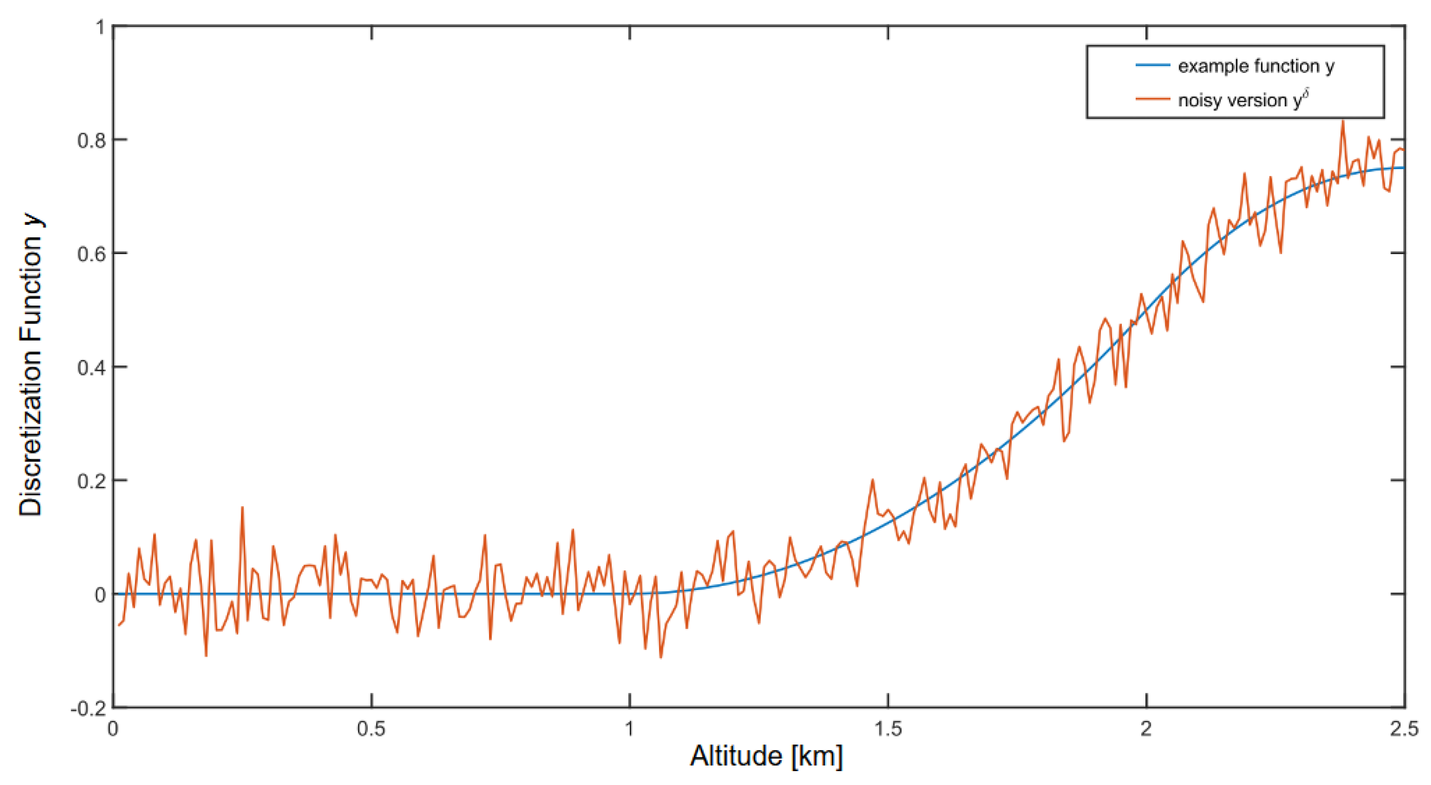
Appendix C. Simple Example with Gaussian Noise

This section aims to present two issues. On the one hand, we show with a simple example for the conveniences of the readers that, e.g., the standard method symmetric different quotient works unstably for the numerical differentiation of a function, like Equation (A20) (see Figure A1 and Figure A3). On the other hand, we demonstrate the good performance of the presented methods, i.e., differentiation with the Levenberg–Marquardt and Tikhonov–Phillips regularization together with the L-curve parameter choice rule for the numerical differentiation. The following example function should represent a good model of the actual Lidar signal. Hence, an “unsmooth” function was chosen. Furthermore, the data were perturbed by a Gaussian noise, which is a good model for the actual noise in the Lidar signal that comes from sun and star light. The example function is given as a discretization of
y : s 0 s 1 0.5 s 2 s + 0.5 1 < s 2 s 2 + 5 s 5.5 2 < s
whereby an equidistant grid of 250 points (0.01 grid-width) over the interval [ 0 , 2.5 ] km was chosen. The function was disturbed at each point by a Gaussian noise Z N ( 0 , 0.05 ) . The corresponding function is shown in Figure A1.
The noise is relatively small. However, it can be seen in Figure A3 that an unregularized solution, e.g., obtained with the symmetric difference quotient, becomes extremely noisy. Compared with this, we see that the regularized solutions obtained by the Tikhonov–Phillips or Levenberg–Marquardt method (methods 2a and 2b) perform much better. In this case, both methods produce nearly the same solution. Furthermore, both L-curves have a similar paths (cf. Figure A2). Besides the “solution” with huge amplitudes of the standard method, this method cannot find the sharp bend at t = 2 .
Figure A1. Example function y from Equation (A20) and its noisy version y δ (red line).
Remotesensing 17 00841 g0a1
Figure A2. L-curves corresponding to the classical Tikhonov–Phillips and the variable Levenberg–Marquardt regularization methods applied to the noisy data y δ . The scaling of the residual norm (horizontal axis) and of the solution norm (vertical axis) is log-converted as explained in Section 2. Both L-curves have almost identical paths and, hence, also almost identical L-corners. Note that a similar position of the L-corner does only imply that both solutions do have the same residual and solution norm. It is always possible that both methods differ at some point.
Remotesensing 17 00841 g0a2
Figure A3. Numerical derivative x of the example function y calculated by three different methods with the noisy function y δ (1 unstable standard method (gray line with reduced scaling by factor 10) and 2 stable regularization methods (red and blue lines)) and the exact analytical derivative of function y (black line).
Remotesensing 17 00841 g0a3

Appendix D. Additional Lidar Application Figures and Tables

Figure A4. This flowchart displays a schematic approach on how to use method 3 to derive an extinction profile. A blue box is a specific object or state that is either given a priori (i.e., the three input boxes) or derived by a task. The tasks are represented by the green and red boxes and well described throughout the paper. The red actions, especially adapting the hyperparameters, indicate that this task requires some experience with the methods. Here, hyperparameters stand for the various options that can be specified in the algorithm (cf. Section 2.2, Section 2.3 and Section 2.4), as for, example, the range of regularization parameters, the step width in the Levenberg–Marquardt method, and the variables k up and k down , which specify how much the part-intervals should overlap. Those yet somewhat difficult tasks might be further simplified or even automated in future work. The first task “Derive an initial interval separation” is described in Section 2.2. If the solutions are not similar, that could indicate an inappropriate choice of the hyperparameters. In this case, the range of the possible regularization parameters has to be adapted. Additionally, if the solutions seem to be under- or over-smoothed, the hyperparameters and interval selection must be adapted. Negative values or rough jump points between part-intervals indicate under-smoothing.
Remotesensing 17 00841 g0a4
Figure A5. (Left) Lidar profile of the 387 nm Raman channel from 28 March 2022, 08:02 UT (blue line), and corresponding synthetic Lidar profile (red line). The synthetic Lidar profile was obtained by the evaluation of the Lidar Equation (2) with an extinction profile computed from the real Lidar profile (blue line) with method 3b. This extinction profile is shown in the (right) Figure.
Remotesensing 17 00841 g0a5
Figure A6. Backscatter coefficient from 28 March 2022, 08:02 UT, for λ = 532 nm light computed with Klett’s method.
Remotesensing 17 00841 g0a6
Figure A7. Extinction coefficients for λ = 532 nm and multiple time steps computed with the variable Levenberg–Marquardt method. (Left) The solution was computed by separating the interval a priori (method 3b). (Right) The solution was computed for the whole interval (method 2b).
Remotesensing 17 00841 g0a7
Figure A8. Extinction coefficients for λ = 355 nm and multiple time steps computed with the Levenberg–Marquardt method and separated intervals. (Left) The regularization parameters are chosen by the L-curve method. (Right) The regularization parameter for the first interval was fixed at k = 40 iterations.
Remotesensing 17 00841 g0a8
Table A1. Parameters settings for the computation of the regularized extinction for λ = 532 nm on 28 March 2022, 08:02 UTC, with the variable Levenberg–Marquardt method. The first row states the parameter settings for method 2b (cf. Figure 6(left)). The second row displays the parameter settings that were chosen for method 3b with part-intervals [ 750 , 2000 ] , [ 2000 , 4000 ] and [ 4000 , 5500 ] m (cf. Figure 6(right)).
k down k up Step Sizes γ Iterations per Step Size
101001 × 10−6, 1 × 10⁻⁵,
1 × 10⁻⁴
10
10301 × 10−7, 1 × 10⁻⁶,
1 × 10⁻⁵, 1 × 10⁻⁴
20
Table A2. Parameter settings for the computation of the regularized extinction for λ = 532 nm on 28 March 2022, 08:02 UTC, with the Tikhonov–Phillips regularization. The first row states the parameter settings for method 2a (cf. Figure 6(left)). The second row displays the parameter settings that were chosen for method 3a with separated intervals [ 750 , 2000 ] , [ 2000 , 4000 ] and [ 4000 , 5500 ] m (cf. Figure 6(right)).
k down k up Exponents x of Reg. Param. 10 x
1010040 equidistant values from [ 4 , 7 ]
1030100 equidistant values from [ 3 , 7 ]
Table A3. Regularization parameters corresponding to the AOD for λ = 355 nm on 2 August 2019, 15:17 UT, computed with the Levenberg–Marquardt regularization and a posteriori SI (method 4b).
Interval [m]Regularization Parameter (Number of Iterations)Curvature at L-Corner
[ 697 , 2860 ] 19 8.93
[ 2860 , 4329 ] 10 4.51
[ 4329 , 6023 ] 8 0.95
[ 6023 , 6817 ] 4 0.12
[ 6817 , 8661 ] 6 0.052
[8661, 10,220]3 0.0017
Table A4. Regularization parameters corresponding to the AOD for λ = 355 nm on 2 August 2019, 15:17 UT, computed with the Tikhonov–Phillips regularization and a posteriori SI (method 4a).
Interval [m]Regularization ParameterCurvature at L-Corner
[ 697 , 2860 ] 6.43 × 10+3 7.99
[ 2860 , 5266 ] 8.70 × 10+4 2.41
[ 5266 , 6847 ] 1.83 × 10+5 0.35
[ 6847 , 9403 ] 7.39 × 10+5 0.05
[ 9403 , 9995 ] 1.00 × 10+7 0.0003
Table A5. Regularization parameters corresponding to the AOD for λ = 355 nm on 2 August 2019, 15:17 UT, computed with the Levenberg–Marquardt regularization and a priori SI (method 3a). The SI was determined by finding intervals with equidistant AOD based on Klett’s solution.
Interval [m]Regularization Parameter (Number of Iterations)
[ 754 , 6008 ] 12
[ 6008 , 7792 ] 10
[ 7792 , 8481 ] 15
[ 8481 , 9995 ] 10

References

  1. Lohmann, U.; Feichter, J. Global indirect aerosol effects: A review. Atmos. Chem. Phys. 2005, 5, 715–737. [Google Scholar] [CrossRef]
  2. Masson-Delmotte, V.; Zhai, P.; Pirani, A.; Connors, S.L.; Péan, C.; Berger, S.; Caud, N.; Chen, Y.; Goldfarb, L.; Gomis, M.; et al. Climate change 2021: The physical science basis. In Contribution of Working Group I to the Sixth Assessment Report of the Intergovernmental Panel on Climate Change; Cambridge University Press: Cambridge, UK, 2021; Volume 2, p. 2391. [Google Scholar] [CrossRef]
  3. Li, J.; Carlson, B.E.; Yung, Y.L.; Lv, D.; Hansen, J.; Penner, J.E.; Liao, H.; Ramaswamy, V.; Kahn, R.A.; Zhang, P.; et al. Scattering and absorbing aerosols in the climate system. Nat. Rev. Earth Environ. 2022, 3, 363–379. [Google Scholar] [CrossRef]
  4. Dubovik, O.; Holben, B.; Eck, T.F.; Smirnov, A.; Kaufman, Y.J.; King, M.D.; Tanré, D.; Slutsker, I. Variability of Absorption and Optical Properties of Key Aerosol Types Observed in Worldwide Locations. J. Atmos. Sci. 2002, 59, 590–608. [Google Scholar] [CrossRef]
  5. Nakoudi, K.; Ritter, C.; Böckmann, C.; Kunkel, D.; Eppers, O.; Rozanov, V.; Mei, L.; Pefanis, V.; Jäkel, E.; Herber, A.; et al. Does the intra-Arctic modification of long-range transported aerosol affect the local radiative budget? (a case study). Remote Sens. 2020, 12, 2112. [Google Scholar] [CrossRef]
  6. Myhre, G.; Myhre, C.; Samset, B.; Storelvmo, T. Aerosols and their relation to global climate and climate sensitivity. Nat. Educ. Knowl. 2013, 4, 7. [Google Scholar]
  7. Weitkamp, C. Lidar: Range-Resolved Optical Remote Sensing of the Atmosphere; Springer Series in Optical Sciences; Springer: Berlin/Heidelberg, Germany, 2005. [Google Scholar] [CrossRef]
  8. Foken, T. Springer Handbook of Atmospheric Measurements; Springer Nature: Berlin/Heidelberg, Germany, 2021. [Google Scholar] [CrossRef]
  9. Böckmann, C. Hybrid regularization method for the ill-posed inversion of multiwavelength lidar data in the retrieval of aerosol size distributions. Appl. Opt. 2001, 40, 1329–1342. [Google Scholar] [CrossRef]
  10. Veselovskii, I.; Kolgotin, A.; Griaznov, V.; Müller, D.; Franke, K.; Whiteman, D.N. Inversion of multiwavelength Raman lidar data for retrieval of bimodal aerosol size distribution. Appl. Opt. 2004, 43, 1180–1195. [Google Scholar] [CrossRef]
  11. Müller, D.; Wandinger, U.; Ansmann, A. Microphysical particle parameters from extinction and backscatter lidar data by inversion with regularization: Simulation. Appl. Opt. 1999, 38, 2358–2368. [Google Scholar] [CrossRef] [PubMed]
  12. Böckmann, C.; Ritter, C.; Graßl, S. Improvement of Aerosol Coarse-Mode Detection through Additional Use of Infrared Wavelengths in the Inversion of Arctic Lidar Data. Remote Sens. 2024, 16, 1576. [Google Scholar] [CrossRef]
  13. Böckmann, C.; Kirsche, A. Iterative regularization method for lidar remote sensing. Comput. Phys. Commun. 2006, 174, 607–615. [Google Scholar] [CrossRef]
  14. Ansmann, A.; Riebesell, M.; Weitkamp, C. Measurement of atmospheric aerosol extinction profiles with a Raman lidar. Opt. Lett. 1990, 15, 746–748. [Google Scholar] [CrossRef]
  15. Pornsawad, P.; Böckmann, C.; Ritter, C.; Rafler, M. Ill-posed retrieval of aerosol extinction coefficient profiles from Raman lidar data by regularization. Appl. Opt. 2008, 47, 1649–1661. [Google Scholar] [CrossRef]
  16. Pornsawad, P.; D’Amico, G.; Böckmann, C.; Amodeo, A.; Pappalardo, G. Retrieval of aerosol extinction coefficient profiles from Raman lidar data by inversion method. Appl. Opt. 2012, 51, 2035–2044. [Google Scholar] [CrossRef] [PubMed]
  17. Ceolato, R.; Berg, M.J. Aerosol light extinction and backscattering: A review with a lidar perspective. J. Quant. Spectrosc. Radiat. Transf. 2021, 262, 107492. [Google Scholar] [CrossRef]
  18. Hu, M.; Li, S.; Mao, J.; Li, J.; Wang, Q.; Zhang, Y. Novel Inversion Algorithm for the Atmospheric Aerosol Extinction Coefficient Based on an Improved Genetic Algorithm. Photonics 2022, 9, 554. [Google Scholar] [CrossRef]
  19. Hoffmann, A. Comparative Aerosol Studies based on Multi-wavelength Raman LIDAR at Ny-Ålesund, Spitsbergen. Ph.D. Thesis, Universität Potsdam, Potsdam, Germany, 2010. [Google Scholar]
  20. Ritter, C.; Münkel, C. Backscatter lidar for aerosol and cloud profiling. In Springer Handbook of Atmospheric Measurements; Springer: Berlin/Heidelberg, Germany, 2021; pp. 683–717. [Google Scholar]
  21. Thorsen, T.J.; Fu, Q.; Newsom, R.K.; Turner, D.D.; Comstock, J.M. Automated retrieval of cloud and aerosol properties from the ARM Raman lidar. Part I: Feature detection. J. Atmos. Ocean. Technol. 2015, 32, 1977–1998. [Google Scholar] [CrossRef]
  22. Ansmann, A.; Wandinger, U.; Riebesell, M.; Weitkamp, C.; Michaelis, W. Independent measurement of extinction and backscatter profiles in cirrus clouds by using a combined Raman elastic-backscatter lidar. Appl. Opt. 1992, 31, 7113–7131. [Google Scholar] [CrossRef] [PubMed]
  23. Bakushinskii, A. Remarks on choosing a regularization parameter using the quasi-optimality and ratio criterion. USSR Comput. Math. Math. Phys. 1984, 24, 181–182. [Google Scholar] [CrossRef]
  24. Kirsche, A.; Böckmann, C. Padé iteration method for regularization. Appl. Math. Comput. 2006, 180, 648–663. [Google Scholar] [CrossRef]
  25. Böckmann, C.; Pornsawad, P. Iterative Runge–Kutta-type methods for nonlinear ill-posed problems. Inverse Probl. 2008, 24, 025002. [Google Scholar] [CrossRef]
  26. Ritter, C.; Burgos, M.A.; Böckmann, C.; Mateos, D.; Lisok, J.; Markowicz, K.; Moroni, B.; Cappelletti, D.; Udisti, R.; Maturilli, M.; et al. Microphysical properties and radiative impact of an intense biomass burning aerosol event measured over Ny-Ãlesund, Spitsbergen in July 2015. Tellus B Chem. Phys. Meteorol. 2018, 70, 1–23. [Google Scholar] [CrossRef]
  27. Dube, J.; Böckmann, C.; Ritter, C. Lidar-Derived Aerosol Properties from Ny-Ålesund, Svalbard during the MOSAiC Spring 2020. Remote Sens. 2022, 14, 2578. [Google Scholar] [CrossRef]
  28. Graßl, S.; Ritter, C.; Schulz, A. The Nature of the Ny-Ålesund Wind Field Analysed by High-Resolution Windlidar Data. Remote Sens. 2022, 14, 3771. [Google Scholar] [CrossRef]
  29. Klett, J.D. Lidar inversion with variable backscatter/extinction ratios. Appl. Opt. 1985, 24, 1638–1643. [Google Scholar] [CrossRef]
  30. Graßl, S.; Ritter, C. Properties of Arctic Aerosol Based on Sun Photometer Long-Term Measurements in Ny-Ålesund, Svalbard. Remote Sens. 2019, 11, 1362. [Google Scholar] [CrossRef]
  31. Hansen, P.C. Analysis of Discrete Ill-Posed Problems by Means of the L-Curve. SIAM Rev. 1992, 34, 561–580. [Google Scholar] [CrossRef]
  32. Hansen, P.C. The L-Curve and Its Use in the Numerical Treatment of Inverse Problems; WIT Press: Southampton, UK, 2001; Volume 4, pp. 119–142. [Google Scholar]
  33. Wahba, G. Spline Models for Observational Data. Reg. Conf. Ser. Appl. Math. 1990, 59. [Google Scholar] [CrossRef]
  34. Kaipio, J.; Somersalo, E. Statistical and Computational Inverse Problems; Applied Mathematical Sciences; Springer: New York, NY, USA, 2010. [Google Scholar] [CrossRef]
  35. Suuronen, J.; Soto, T.; Chada, N.K.; Roininen, L. Bayesian inversion with α-stable priors. Inverse Probl. 2023, 39, 105007. [Google Scholar] [CrossRef]
  36. Engl, H.W.; Hanke, M.; Neubauer, A. Regularization of Inverse Problems; Mathematics and Its Applications; Springer: Dordrecht, The Netherlands, 2000. [Google Scholar] [CrossRef]
  37. Kirsch, A. An Introduction to the Mathematical Theory of Inverse Problems; Springer Nature: Cham, Switzerland, 2021. [Google Scholar] [CrossRef]
Figure 1. Location of Ny-Ålesund with our Lidar system on the west coast of Spitsbergen in the European Arctic. Sources: https://geokart.npolar.no/Html5Viewer/index.html?viewer=Svalbardkartet and https://de.wikipedia.org/wiki/Datei:Europe_on_the_globe_(red).svg (last accessed: 20 February 2025).
Remotesensing 17 00841 g001
Figure 2. (Left) Signal P607analog from 28 March 2022, 08:02 UT, in an arbitrary unit. (Right) Corresponding term y, the cumulative total optical depth.
Remotesensing 17 00841 g002
Figure 3. (Left) Synthetic Lidar profile (red line) and 20 versions of perturbations by artificial noise. The synthetic Lidar profile is obtained from the extinction of the 387 nm channel from 28 March 2022, 08:02 UT (cf. Figure A5). (Right) Extinction profile corresponding to the synthetic Lidar profiles with artificially created noise. Profiles were obtained by averaging over the solutions from the 20 signals shown in the right Figure. These solutions were computed with regularization method 3b (magenta line) and without any regularization method (cyan line).
Remotesensing 17 00841 g003
Figure 4. (Left) Extinction profiles of the 20 artificial noisy Lidar profiles shown in Figure 3(left) computed with the Levenberg–Marquardt method and a priori SI (method 3b). (Right) Pointwise maximum and mean deviation between the artificial extinction profiles from the left figure and the original extinction profile that was obtained from the real Lidar signal (cf. Figure A5).
Remotesensing 17 00841 g004
Figure 5. Plot of the BSR on 28 March 2022 obtained with Klett’s method. The Lidar ratio was chosen to be 50 sr.
Remotesensing 17 00841 g005
Figure 6. Regularized solutions of extinction coefficient for λ = 532 nm from 28 March, 08:02 UT. (Left) Solutions are computed for the interval [ 750 , 5500 ] m at once, i.e., methods 2a and 2b. (Right) Solutions with a priori SI [ 750 , 2000 ] , [ 2000 , 4000 ] , and [ 4000 , 5500 ] m, i.e., methods 3a and b.
Remotesensing 17 00841 g006
Figure 7. L-curves corresponding to the regularized extinctions profiles (Figure 6) for λ = 532 nm from 28 March 2022, 08:02 UTC. (Left) L-curves for solutions computed with methods 2a and 2b (Figure 6(left)). (Right) L-curves for solutions computed with methods 3 and 4 (Figure 6(right)). The left-most curves correspond to the interval [ 700 , 2000 ] m, the centred curves to the interval [ 2000 , 4000 ] m, and the right curves to the interval [ 4000 , 5500 ] m.
Remotesensing 17 00841 g007
Figure 8. (Left): Horizontal wind speed. (Right) Wind speed direction on 28 March 2022.
Remotesensing 17 00841 g008
Figure 9. Average extinction profiles of λ = 355 nm light from 28 March 2022. The solutions for each time step were calculated with the Levenberg–Marquardt method with a posteriori SI (method 4a). Since the regularization parameter α L at the L-corner seems to produce under-smoothed solutions (cf. Figure A8), the L-corner algorithm was modified. Instead of α L , the algorithm chooses min ( 3 , α L 5 ) .
Remotesensing 17 00841 g009
Figure 10. Vertical wind speed on 28 March 2022.
Remotesensing 17 00841 g010
Figure 11. AOD retrieved from λ = 355 nm light on 2 August 2019. Solutions were computed with Klett’s method [29].
Remotesensing 17 00841 g011
Figure 12. (Left) Signal P387analog and a smoothed signal P387 from 2 August 2019, 15:05 UT, in arbitrary units. (Right) Corresponding terms y (the cumulative total optical depth).
Remotesensing 17 00841 g012
Figure 13. Different solutions for the cumulative AOD for λ = 355  nm from 2 August 2019, 15:17 UT. The decomposed data of Y are an AOD, directly obtained from the total cumulative AOD Y, as described in Equation (22). Together with Klett’s solution (taken from Figure 11), it serves as a comparison with our methods. The red solution is obtained with the variable Levenberg–Marquardt method applied to the hole interval [750, 10,000 m] (method 2b). It uses the signal P387analog. The yellow graph was computed with the same method but with a smoothed version of the signal P387analog. All the other methods use again the original signal P387analog. The green graph is the solution computed with the variable Levenberg–Marquardt method with an a priori SI (method 3b). In this case, the part-intervals were chosen such that every interval contains approximately the same AOD based on Klett’s solution. The last two solutions (purple and blue lines) are obtained with methods 4a and 4b (a- posteriori SI).
Remotesensing 17 00841 g013
Figure 14. (Left) Signal P387analog from 18 October 2021, 20:46 UT, in arbitrary units. (Right) Corresponding term y, the cumulative total optical depth.
Remotesensing 17 00841 g014
Figure 15. Different solutions for the extinction of λ = 355 nm light on 18 October 2021, 20:46 UT. The solution was always computed with the Levenberg–Marquardt method, and the interval separation (method 3a) is given in the titles. The red dashed lines mark the altitudes, where we split the interval for the following solution. (a) Solution was computed over the whole interval [ 700 , 6000 ] m. We recognize a cloud between 1900 m and 2600 m. (b) This solution shows that the cloud is even thinner and must lie between 2100 m and 2800 m. (c) Detailed features of the cloud are visible in this plot. To obtain an even more precise solution, we separate the middle interval into three smaller intervals to isolate the peaks of the cloud. (d) Final solution obtained by the previous determined interval separation. The solution is compared with the classical Ansmann solution (method 1).
Remotesensing 17 00841 g015
Figure 16. Cumulative AOD corresponding to the different solutions for the extinction of λ = 355 nm light on 18 October 2021, 20:46 UT, from Figure 15. The lines (a–d) correspond to the extinction profiles in Figure 15a–d, respectively.
Remotesensing 17 00841 g016
Figure 17. Comparison of the retrieval of mean extinction profiles for 532 nm and the case of 28 March 2022; compare Section 3.2. The profiles were averaged over six time steps between 08:02 and 08:59 UT. The clear improvement compared with the non-regularized solution (green, method 1) is evident.
Remotesensing 17 00841 g017
Figure 18. Signal-to-noise ratio of the 607 nm Raman channel for the case of 28 March 2022; compare Section 3.2.
Remotesensing 17 00841 g018
Table 1. Comparison of the different methods that were used throughout the paper. The four methods refer to the non-regularized “Ansmann solution” (1), regularized solution of the whole altitude range (no selection of part-intervals) (2), regularization with an a priori selection of the intervals (3), and regularization with an a posteriori selection of the intervals (4).
MethodDescription/Use CasesWeaknesses/Difficulties
1
  • Classic approach
  • Assumes that data are noise-free
  • Only works for data with high SNR (mostly low altitudes or might time conditions)
  • Does not perform well if data are noisy (no regularization used)
2
  • Works well for small intervals
  • Can be used to estimate aerosol peaks in a large interval (cf. Figure 15a).
  • Since we do not split the interval, there is no risk of getting jumps in the solution from sticking two solutions together
  • Solution is rather a rough estimate and often over-smoothed in the left half of the interval
3
  • Splitting the interval is a way to include a priori information as, e.g., the SNR or AOD estimated from Klett’s method
  • Different regularization parameters for each part-interval are computed. Each regularization parameter fits better to the certain SNR in that part-interval.
  • Can be used to iteratively identify sharp transitions in the extinction profile (cf. Section 3.4)
  • If suitable interval split was found, it often applies well for successive time steps
  • Potentially unrealistic jumps at the points, where we stick the solution to part-intervals together due to uncertainties of the solution at the end of each part-interval.
  • This effect is even worse if we average over multiple solutions of successive time steps, where we used the same interval split for each solution
4
  • Chooses interval split automatically, does not rely on a priori heuristics
  • If used for successive time steps, it will produce slightly different interval splits for each time. Hence, it is good to compute time-averaged profiles as uncertainties at the points, where we stick part-intervals together, is averaged out (cf. Figure 9)
  • Requires choice of additional hyperparameters, as, for example, the minimal and maximal length of a part-interval
  • In general, it is more difficult to tune the hyperparameters. The solution seems to be more sensitive with respect to changes in the hyperparameters compared with methods 2 and 3
Disclaimer/Publisher’s Note: The statements, opinions and data contained in all publications are solely those of the individual author(s) and contributor(s) and not of MDPI and/or the editor(s). MDPI and/or the editor(s) disclaim responsibility for any injury to people or property resulting from any ideas, methods, instructions or products referred to in the content.

