Abstract
The orthogonality of transmitted waveforms is an important factor affecting the performance of MIMO radar systems. The orthogonal coded signal is a commonly adopted waveform in MIMO radar, and its orthogonality depends on the used orthogonal discrete code sequence set (ODCSs). Among existing optimization algorithms for ODCSs, the results designed by the greedy code search-based memetic algorithm (MA-GCS) have exhibited the best autocorrelation and cross-correlation properties observed so far. Based on MA-GCS, we propose a novel hybrid algorithm called the memetic algorithm with iterative greedy code search (MA-IGCS). Extensions involve replacing the greedy code search used in MA-GCS with a more efficient approach, iterative greedy code search. Furthermore, we propose an “individual uniqueness strategy” and incorporate it into our algorithm to preserve population diversity throughout iteration, thereby preventing premature stagnation and ensuring the continued pursuit of feasible solutions. Finally, the design results of our algorithm are compared with the MA-GCS. Experimental results demonstrate that the MA-IGCS exhibits superior search capability and generates more favorable design results than the MA-GCS.
1. Introduction
Multiple-input multiple-output (MIMO) radar has attracted significant interest owing to its exceptional capabilities in target detection and parameter estimation [1,2,3]. Selecting suitable waveforms is crucial for unlocking the full potential of MIMO radar systems and achieving excellent performance. Currently, commonly employed MIMO radar waveforms can be broadly categorized into four types: (1) time division multiple access (TDMA), (2) frequency division multiple access (FDMA), (3) code division multiple access (CDMA), and (4) Doppler division multiple access (DDMA) [2,3].
Each of these four MIMO radar waveforms has its benefits and drawbacks [4]. Among them, TDMA-MIMO radar waveform, due to its inefficient use of multi-channel transmission capabilities, results in a shorter radar detection range compared to other radar waveforms. Nevertheless, its advantage is reflected in its straightforward channel separation [1,5,6,7]. Application of the FDMA-MIMO waveform also achieves favorable orthogonal properties. However, the complex implementation structure limits its wide application in millimeter-wave radar chips [1,5,8]. The DDMA-MIMO waveform possesses good orthogonality and can achieve complete separation in the Doppler domain. On the other hand, it faces a limited Doppler unambiguity range, which reduces the detectable velocity range of moving targets [1,9,10]. The advantage of the CDMA-MIMO waveform is that it can approximately satisfy the orthogonality requirement through phase or frequency modulation without loss of transmit power, bandwidth, or pulse duration. However, one drawback of CDMA-MIMO radar waveforms is that their orthogonality is determined by orthogonal discrete code sequence set (ODCSs); since ODCSs with both ideal autocorrelation and cross-correlation properties do not exist, the orthogonality of CDMA-MIMO radar waveforms is not as good as that of other waveforms [3,6]. Therefore, the design and optimization of ODCSs is crucial to exploiting the potential of CDMA-MIMO radar waveforms.
Moreover, the design and optimization of ODCSs is a complex, high-dimensional, NP-complete problem. The computational cost of optimization for a code set with code set size L, code length N, and optional phase number M is on the order of , the computational cost growing exponentially with code set size L, code length N [11]. Conventional and classical optimization methods are not efficient enough to deal with such a complex, high-dimensional, NP-complete problem [12]. To address the challenge of optimizing ODCSs, various approaches have been proposed, including meta-heuristic algorithms, algebraic methods, and deep learning techniques [13,14,15]. Meta-heuristic algorithms have received widespread attention for their remarkable efficiency in solving optimization problems, ease of development, and other advantages [16]. The proposed meta-heuristic algorithms can be further divided into evolution-based, physics-based, or swarm intelligence-based [12]. Examples include the genetic algorithm [17], simulated annealing [11], particle swarm optimization [18], ant colony optimization [19,20], and a host of other algorithms [21].
The most used meta-heuristic algorithm for ODCSs optimization and various branches developed from it will be discussed here to be the starting point of our work. For brevity, other methods such as algebraic methods and deep learning will no longer be elaborated. A hybrid optimization algorithm combining a simulated annealing algorithm and a greedy code search algorithm was first proposed in ref. [11], which provides an effective method to solve the problems mentioned above. Subsequently, Liu et al. [22] proposed a hybrid genetic algorithm that integrates greedy code search algorithm. The method introduces genetic algorithm into the optimization problem of multiphase code sets for the first time, which provides a powerful tool and a new idea for the design of orthogonal multiphase sequences. Design results of this method show apparent progress in the performance of the polyphase code set compared to the design results in ref. [11]. Aiming at the two main defects of classical particle swarm optimization algorithm, the convergence problem and failure to deal with high-dimensional optimization problems, Zeng et al. presented a novel multi-objective micro particle swarm optimization (MO-MicPSO) method, which is characterized by using only a small population size to solve high-dimensional multi-objective optimization problems [18]. In ref. [20], the author focuses on the issue of optimizing discrete frequency coding waveform sequences in MIMO radar systems and develops an “improved ant colony optimization” algorithm. The algorithm finds optimal waveform sets by simulating foraging behavior of an ant colony and then compares results with other methods to illustrate its high efficiency and superior performance in searching large sets of waveforms. A greedy code search-based memetic algorithm (MA-GCS) is presented in ref. [23]. MA-GCS is a combination of an evolutionary algorithm and a greedy code search algorithm, which further improves the exploration and exploitation capabilities of optimization algorithms. In addition, the authors design an acceleration algorithm to reduce the computational complexity of local search. Experimental results given in the paper show that code sets designed by this algorithm have better autocorrelation and cross-correlation performance than other methods.
Although meta-heuristic algorithms as described above and a series of other proposed optimization algorithms have achieved good optimization results, there are still some problems that need to be solved, such as premature convergence and local search efficiency. In this situation, an effective algorithm is developed for the design of ODCSs in this paper. Iterative greedy code search is introduced into algorithm framework which is an extension of greedy code search. It conducts multiple local searches on the resulting offspring until the objective function no longer decreases. As a result, iterative greedy code search delivers superior search results compared to GCS at the same number of global searches. In addition, we propose an “individual uniqueness strategy” to prevent the algorithm from premature convergence. Hence, the performance of ODCSs designed with this method is much closer to the theoretical lower bound.
This paper is structured as follows: In Section 2, we introduce the problem of designing the ODCSs and outline the evaluation criteria for the code sequence sets. Section 3 details the iterative greedy code search strategy, a method for preserving population diversity, and the algorithmic flow of the whole algorithm. Section 4 presents the algorithm’s design outcomes and compares them with previous methods. Finally, Section 5 is a summary of this paper.
2. Problem and Materials
In order to understand thoroughly the problem to be addressed, we first introduce the concept of ODCSs and then state the problem of designing ODCSs.
The use of orthogonal waveforms can minimize the mutual interference between different transmitted signals. However, achieving ideal orthogonal waveforms is not feasible without sacrificing transmitted power, bandwidth, or other resources [24]. Therefore, “orthogonal” in this paper refers to “approximate orthogonal” not “ideal orthogonal”; i.e., it has good autocorrelation and cross-correlation properties. To promote the target detection performance of CDMA radar by means of waveform design, the key is to improve cross-correlation performance of the ODCSs while maintaining good autocorrelation characteristics.
2.1. Problem Statement
In this part, the design problem related to the ODCSs will be elaborated. The waveforms that achieve orthogonality through coding diversity can be either fast-time coded signals (intra-pulse coded waveform) or slow-time coded signals (inter-pulse coded waveform). Here, we consider a frame of the slow-time polyphase coded signal, in which a frame of the signal is composed of N pulses. Assume a MIMO radar system has L transmitting antennas and each transmits a frame of the slow-time polyphase coded signal, which can be expressed as follows:
where S represents set of L-frame signals transmitted by L transmitting antennas, i.e., S contains pulses. is the nth signal transmitted by the lth antenna. is transmitted signal waveform, which can be a linear frequency modulation (LFM) signal, a single-frequency continuous wave signal, etc., and is phase modulation function whose value can only be selected from (2), where M is the distinct phase number.
Formula (2) shows that the phases of the ODCSs are taken discretely, and there are only M optional discrete phases. Moreover, each phase in Formula (2) can be replaced by a number before , as shown in Formula (3). Taking binary code as an example, the optional phase of is 0 or , and corresponding discrete numbers are 0 and 1, respectively.
Similar to the value restriction in Formula (2), can only be chosen from the listed values in (3), with each discrete number in (3) corresponding to each phase value in (2) one by one.
When a transmitted signal waveform is determined, S can be concisely represented with an matrix as:
Although three different forms of S are substantially the same and can be converted into each other, each form has unique advantages and is suitable in different scenarios. Therefore, it is necessary to choose the appropriate form according to specific situations. is commonly used in optimization processes as this form eases the calculation of the objective function. The advantage of is that its representation is very intuitive and often used in data analysis. The last form appears more often in particle swarm optimization algorithms since these algorithms use discrete numbers to represent the current positions of particles. In our proposed algorithm, the first form is used during algorithm iteration for computational convenience. Moreover, in the experimental results analysis section, we use the second form to show the obtained ODCSs. In some cases, the three forms may all be used, such as in the improved ion motion algorithm proposed in ref. [25].
Based on the representations given above, the aperiodic autocorrelation and cross-correlation function of the ODCSs are defined as:
where is the aperiodic autocorrelation function of sequence in the ODCSs and is the aperiodic cross-correlation function of sequences and in the ODCSs. k denotes discrete time lag, and represent the nth element and th element of the lth sequence, respectively. denotes normalization of the above two correlation functions, where N is code length of the chosen sequence. The main purpose of performing normalization is to facilitate comparison of subsequent experimental results.
Many evaluation metrics have been proposed to evaluate the performance of the ODCSs. Among these, the peak sidelobe level (PSL) and integrated sidelobe level (ISL) are commonly used. Peak sidelobe level consists of cross-correlation peak (CP, largest magnitude of cross-correlation over all shifts), autocorrelation sidelobe peak (ASP, largest magnitude of autocorrelation sidelobe over all shifts except shift 0, i.e., ) [26,27]. Their definitions are shown below:
From the above formulas, it can be seen that ISL is the sum of the squares of correlation function values (autocorrelation function values and cross-correlation function values), excluding autocorrelation function values at . In brief, ISL reflects overall characteristics of correlation function. PSL is the maximum value in N autocorrelation sidelobe peaks and cross-correlation peaks, reflecting local characteristics of correlation function.
2.2. Evaluation Criterion
To gain an overall perspective of the optimization problem to be investigated, we provided expression for the ODCSs, derived formulas for calculating autocorrelation function and cross-correlation function of the ODCSs and introduced the evaluation metrics for the performance of the ODCSs in the preceding sections. Now, we will discuss the objective function.
Generally speaking, the choice of objective function decides whether the solution of an optimization problem is the expected one. To obtain the ODCSs with better orthogonality, this paper takes the weighted sum of the autocorrelation sidelobe peak and cross-correlation peak as the objective function, as shown in (13).
where w is the weighting coefficient to trade off the impact of the autocorrelation sidelobe peak and cross-correlation peak, with a value ranging from 0 to 1. That is to say, a bigger w indicates that the autocorrelation sidelobe peaks of the code sequences take higher priority in the optimization process and vice versa. According to the definition in (13), it can be observed that the objective function reflects a comprehensive impact of the autocorrelation and cross-correlation functions. Therefore, the smaller the objective function is, the better the orthogonality of ODCSs is. To evaluate the orthogonality of the ODCSs, average ASP (A-ASP) or average CP (A-CP) are applied, which can be calculated as follows.
3. MA-IGCS for Optimization of ODCSs
The optimization method proposed in this paper adopts the memetic algorithm framework, which employs evolutionary algorithm and the iterative greedy code search strategy in the global and local levels respectively. Therefore, in this section, we first present an introduction to the memetic algorithm framework. Subsequently, an iterative greedy code search strategy and a method to maintain population diversity are proposed in Section 3.2 and Section 3.3. In Section 3.4, the detailed algorithmic flow of the optimization algorithm (i.e., the memetic algorithm with iterative greedy code search, MA-IGCS) proposed in this paper is given. Finally, the time complexity of the MA-IGCS is derived in Section 3.5.
3.1. Memetic Algorithm
3.1.1. Introduction to MA
The memetic algorithm (MA) is a combination of population-based global search and heuristic local search made by each individual [28]. In ref. [28], the author points out that the motivation for genetic algorithm comes from imitating the optimization of genetic code in biological evolution, while meme algorithms try to mimic the optimization of memes in cultural evolution (in the case of Chinese Kung Fu, for example, those undecomposable movements in martial arts are the memes). The most distinct difference between MA and the genetic algorithm (GA) is that the MA combines global search with individual local search, which enhances the efficiency of solving optimization problems.
The MA has been successfully applied to solve many optimization problems, such as combinatorial optimization [29], non-stationary function optimization [30], multi-objective optimization [31], graph theory [32], the job shop scheduling problem (JSP) [33], FIR filter design [34], and the university course schedule problem [35]. Two typical application instances are the prediction of protein structures and optimal design of spacecraft orbits [36].
In this paper, the MA is used to optimize the ODCSs for the following reasons. Firstly, the ODCSs optimization problems usually need to find excellent solutions in a huge search space. The MA combines the global search ability and the local search, which can effectively explore and develop potential high-quality solutions in the search space. In addition, it proposes a new algorithmic framework, which can integrate and utilize all previous knowledge of the existing heuristic methods to improve the efficiency of solving complex optimization problems. In conclusion, the MA can effectively cope with the complexity and diversity of ODCSs optimization problems and provide high-quality solutions.
3.1.2. General Form of the Memetic Algorithm
In ref. [36], the authors make a concise and complete introduction to the memetic algorithm and give a more general form of the simple memetic algorithm, and its pseudocode is shown in Algorithm 1.
A population is a set of possible solutions. The population can be generated by simple random creation or using existing solutions. Before initializing the population, a series of parameters, including the maximum number of iterations and the code sequence set parameters, need to be initialized, where code sequence set parameters include sequences number L, code length N, and optional phase number M. Once the population initialization is finished, the objective function will be calculated for each individual in the population. Subsequently, a local search is performed for each individual [23]. After the local search of the initial individual is completed, the evolutionary operations, local searches, and selection operations are repeated until the termination condition is triggered. The goal of the evolutionary operation is to generate new individuals from old individuals through mutation operator or crossover operator. The process of creating new individuals is equivalent to generating new candidate solutions. The selection operator, working at the population level, distinguishes individuals based on their objective function and thereby enables superior individuals to become parents of the descendent generation. Regarding the termination condition, it can be a predefined number of iterations or a threshold value for the objective function.
| Algorithm 1 Pseudocode for a simple memetic algorithm [36] |
|
3.2. Iterative Greedy Code Search Strategy
Greedy code search (GCS), also known as a Hamming scan, first came up in ref. [37] and has been applied in many optimization algorithms [11,22,23]. GCS was originally proposed to obtain good aperiodic binary sequences and is essentially an iterative process based on enumeration and combinatorial structures. It consists of two main steps: element complementation and cyclic permutation. In element complementation, only one element value is changed in each iteration (from +1 to −1 or vice versa), and the corresponding objective function value is calculated. The change that minimizes the objective function value will be kept and used as the starting point for the next iteration. The purpose of cyclic permutation is to explore possible optimized sequences further when a local minimum is reached through element complementation. This step involves recording the first element and performing a cyclic permutation of the remaining elements.
However, the currently used GCS has become quite different from the original version. Firstly, the cyclic permutation is eliminated since changing the arrangement of elements in the code sequence set may deteriorate extremely its orthogonality. Secondly, the element value in the element complementation is extended from binary elements to quaternary, octal, hexadecimal, and other multi-ary elements. After modification, GCS has been widely applied to enhance the ability of pursuing optimal solution. Although the local search capability of GCS is quite powerful, it becomes less effective in the later stages of optimization. To fix this problem, an iterative greedy code search (IGCS) algorithm will be introduced below.
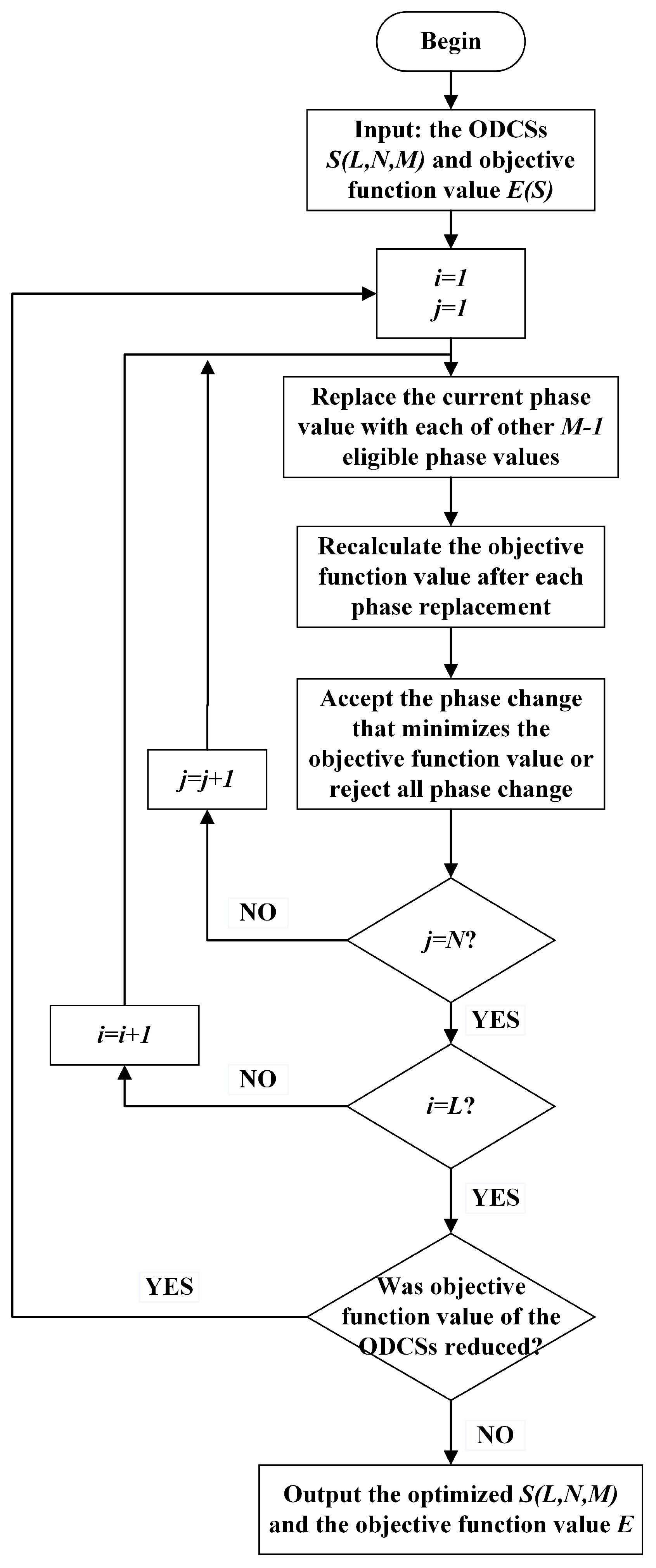
As an extension of the GCS algorithm, the concept of the iterative greedy code search algorithm (IGCS) was first introduced in ref. [11], although the author still refers to it as a GCS algorithm. Then, the specific implementation process of IGCS is introduced. Assuming that the value of in Matrix (5) is , the remaining phase value in (2) is used to replace in turn, and the objective function value of is updated after each replacement. If the objective function value decreases, the new phase value is accepted. Otherwise, the original phase value remains unchanged. After the phase replacement procedure of is completed, the same procedure is performed on in turn. And above the phase replacement procedure constitutes a complete GCS. Subsequently, the GCS is applied to the Matrix (5) repeatedly until the objective function value of cannot become smaller further.
To illustrate the whole procedure, a detailed flowchart is shown in Figure 1. The loop variables i and j in Figure 1 represent sequence numbers and code lengths, respectively.

Figure 1.
Flowchart for optimization of using IGCS.
3.3. Individual Uniqueness Strategy
Population diversity refers to the extent of differences among individuals in a population. High diversity implies that individuals are quite different from each other, while low diversity indicates that individuals tend to be similar. Maintaining population diversity is crucial because it affects the convergence speed and algorithm robustness. MA suffers from loss of diversity owing to premature convergence that the population converges around some sub-optimal points. When this happens, the MA will lose the ability to continue searching for feasible solutions and the optimization comes to a stagnation.
Several approaches have been proposed to solve this problem [36]:
- Enhancing the diversity of the initial population.
- Applying the local search to a small portion of the population (which helps to ensure that the rest of the population is diverse).
- Using a crossover operator designed to maintain diversity.
- Adding multiple local searchers, each of which produces a different search space with different local optima.
- Modifying the selection operator to prevent duplicates.
- Trying the partial restart strategy, the partial restart introduces randomly generated individuals into the current population during the optimization so as to increase the genetic diversity of the population [23].
We propose an “individual uniqueness strategy” inspired by this phenomenon: In some situations, it is observed that optimization sometimes stagnates when only the crossover operator is used to generate offspring during iteration. After analyzing the final optimized population, the reason for the loss of population diversity is identified. Analysis shows that when optimization stagnates there is only one unduplicated individual in the population, resulting from the local optimal individual being repeatedly retained during the selection process. Because of population diversity loss, the crossover operator cannot generate new offspring through swap operations between individuals. The “individual uniqueness strategy” is proposed to ensure that no duplicate individuals exist in the population after selecting operations during each iteration.
Figure 2 is a flowchart of the “individual uniqueness strategy” and followed by its implementation steps. In Figure 2, i and j denote the ith and jth individuals in the population (the jth individual may be retained or deleted), and N is the number of individuals in the population.
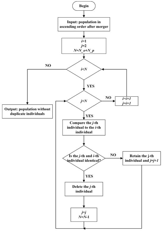
Figure 2.
Flowchart of using “individual uniqueness strategies” to maintain population diversity.
The first step is fusion processing, the parents used and generated offspring in the current iteration are merged. Then, individuals in merged populations are sorted in ascending order according to the value of the objective function. The sorted individuals are compared sequentially to check whether the individuals are duplicates or not. If two individuals are identical, one of the duplicate individuals will be removed; otherwise, it is retained. After removing or retaining the individual, the comparison moves on to the next individual. Ultimately, a refreshed population without duplicate individuals is obtained following a comprehensive comparison of all individuals.
The “individual uniqueness strategy” can enhance the quality of generated offspring and improve optimization results with negligible impact on runtime. Following the execution of the “individual uniqueness strategy”, the next iteration’s parent is selected from the population. Subsequently, the algorithm proceeds to the next iteration and the mutation or crossover operator is employed to produce offspring in subsequent iteration. Reduced population diversity could lead to offspring generated with mutation or crossover operators becoming highly similar. So, without implementing the “individual uniqueness strategy”, all offspring may converge to the same solution after local search, ultimately making the algorithm lose its search ability after multiple iterations.
Maintaining population diversity through the “individual uniqueness strategy” is one of the key advantages of our proposed algorithm, which enables our algorithm to continuously search for feasible solutions.
3.4. Memetic Algorithm with Iterative Greedy Code Search
In Section 3.1, Section 3.2 and Section 3.3, we respectively introduced the memetic algorithm framework, iterative greedy code search strategy, and individual uniqueness strategy. With the foundational knowledge from these preceding subsections, we present the complete memetic algorithm with iterative greedy code search (MA-IGCS). The distinguishing features of our proposed algorithm MA-IGCS compared to others are as follows:
- The MA-IGCS utilizes the MA framework introduced in Section 3.1 as its algorithmic framework, which enables the MA-IGCS to adopt a hybrid search mechanism integrating local search and global search. The hybrid search mechanism allows the MA-IGCS to search effectively on different levels, thereby promoting the convergence speed of the MA-IGCS and the quality of solutions.
- The MA-IGCS adopts the IGCS strategy introduced in Section 3.2 as its local search approach. As an extension of the GCS, the IGCS strategy can find a better local solution through multiple iterations. By utilizing the local solution obtained via the IGCS strategy to gradually improve the solution, the local search capability and search efficiency of the algorithm are lifted up.
- The “individual uniqueness strategy” described in Section 3.3 is implemented in the MA-IGCS to maintain population diversity during each iteration. The search space of our proposed algorithm is expanded by using the “individual uniqueness strategy”, enabling it to continuously search for feasible solutions and ultimately achieve superior solutions.
- In our proposed algorithm, both the mutation operator and crossover operator are employed to generate offspring. The mutation operator generates a new solution by introducing a certain random disturbance to the current solution. On the other hand, the traits (part of the phase value in code set) of desirable individuals will be randomly combined to generate new solutions when using the crossover operator. Two operators generate offspring in different ways, which can prevent the population from converging prematurely to the local optimal solution and increase the possibility of finding the global optimal solution.
The pseudocode for the MA-IGCS is shown below in Algorithm 2.
| Algorithm 2 Pseudocode for MA-IGCS |
|
3.5. Time Complexity Analysis of the MA-IGCS Algorithm
The time spent on the MA-IGCS is composed of the following parts: population initialization, objective function calculation, offspring generation, local search, and generation of new parents. The time complexity of each part is demonstrated below.
- In the first step of population initialization, individuals are generated, where an individual makes assignments, so the time complexity of population initialization is .
- Generation of new individuals from old ones by the mutation operation or crossover operation determines the time complexity related to the procedure of offspring generation. The computational complexity is and , where is the number of mutation bits and is the number of crossover columns. Therefore, .
- The implementation of GCS includes phase replacement and recalculating the objective function after each phase replacement. The objective function update after each phase substitution contributes significantly to the time complexity of the local search. So, when updating the objective function in the local search, we use the acceleration algorithm proposed in ref. [23] to reduce the computational complexity. Furthermore, according to the algorithm simulation results, one IGCS typically includes a GCS, where we use the uncertain integer A to represent . Therefore, its time complexity is . It should be noted that although the constant term is omitted for brevity here, the time consumption of the IGCS is times that of the GCS due to the existence of a constant term.
- The generation of new parents involves merging offspring and parents, sorting the merged population, removing duplicates, and taking the first individuals as parents. Since the time spent on merging and assigning operations is a constant item, the time complexity of new parent generation is determined by the sorting and deletion operations. The computational complexity of sorting and deleting operation is and , respectively. Consequently,
In summary, the time complexity of other parts is far less than and . Moreover, can also be ignored when compared to . Therefore, the time complexity of whole algorithm is mainly controlled by the local search efficiency of newly generated offspring during each iteration. Taking each item into account, the time complexity of MA-IGCS is
To illustrate the effectiveness and efficiency of the proposed algorithm more comprehensively, the time complexity of the SA-IGCS, GA, MSAA, and other algorithms is firstly derived and compared with the MA-IGCS. The results are shown in Table 1.

Table 1.
Comparison of time complexity between MA-IGCS and other existing methods.
In Table 1, A and B are uncertain integers. Our simulation results show that the value range of A is 3∼4, and B is the total number of iterations in the simulated annealing algorithm and its value is usually at a very high order. However, we know that the performance of these heuristic algorithms is greatly affected by the parameter settings. But, the parameters of these algorithms are not all the same, and the time complexity will vary with the parameters. Therefore, based only on the data in Table 1, we cannot draw a convincing conclusion. We will further analyze it in Section 4.2.
4. Simulation Results and Discussion
All simulations presented in this paper are carried out on a computer with an Intel(R) Core(TM) i5-12450H CPU@4.4 GHz, manufactured by Zhihui Tong Intelligent Technology (Suzhou) Co., Ltd., with its research and production base located in Suzhou, Jiangsu Province, China. In this part, we first validate the benefits of introducing IGCS and the “individual uniqueness strategy” through comparative experiments. Then, the design results obtained by the MA-IGCS algorithm are shown and analyzed. Finally, it is compared with other optimization algorithms to show the superiority of the proposed algorithm.
4.1. Benefits of Introducing IGCS and the “Individual Uniqueness Strategy”
Algorithm 2 is adopted as a basic framework, and then the ODCSs with the number of sequences , code length , and optional phase number are the aim of the optimization work. We conducted three experiments: experiment 1 is a control experiment, experiment 2 applies the proposed “individual uniqueness strategy” to the algorithm, and experiment 3 adds an iterative greedy code search method based on experiment 2.
The average autocorrelation sidelobe peak level (A-ASPL) and average cross-correlation peak level (A-CPL) are introduced to compare the performance of the ODCSs obtained by different experiments and algorithms, which are calculated as shown in (17) and (18).
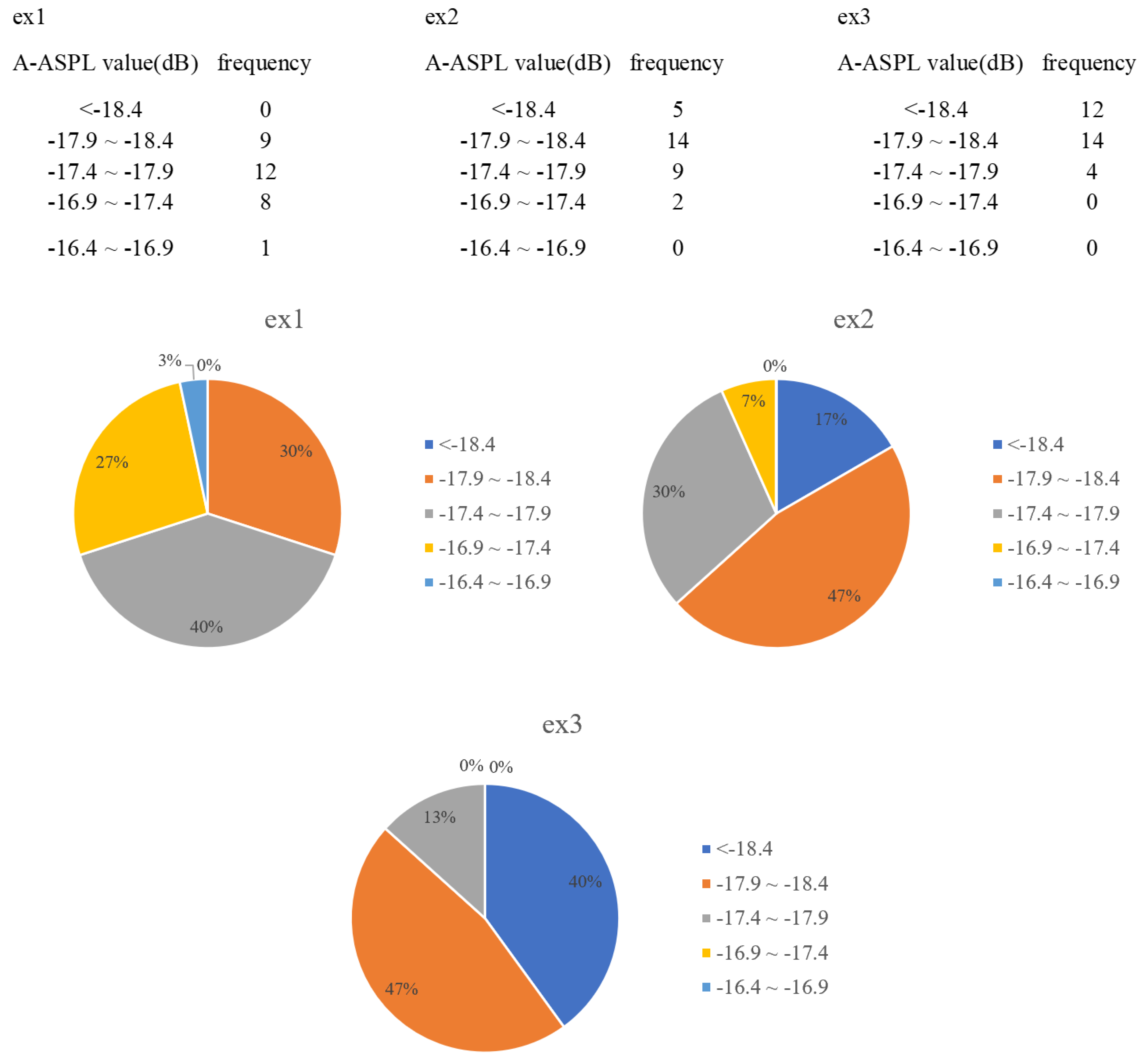
Figure 3 shows the A-ASPL value (dB) frequency distribution table and the corresponding pie chart of the three experiments (ex1, ex2, ex3). The A-ASPL values of each experiment are divided into the same five intervals, as shown in Figure 3. In ex1, the −17.9∼−17.4 dB interval has the highest frequency at 40%, and the interval <−18.4 dB has the lowest frequency at 0%. Ex2 also reaches the highest frequency (47%) in the interval −17.9∼−17.4 dB, and the frequency of interval <−18.4 dB is 17%. Ex3 has the same frequency of 47% as ex2 in the interval −17.9∼−17.4 dB, while its frequency increases from 17% to 40% in the interval <−18.4 dB compared to ex2.
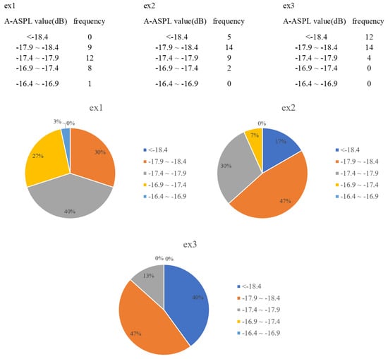
Figure 3.
Comparison of A-ASPL frequency distribution under different experimental conditions.
Figure 4 illustrates the frequency distribution table of A-CPL values and the corresponding pie chart. The A-CPL values are also divided into five intervals, as shown in Figure 4. Ex1 achieves a peak frequency of 40% in the interval of −14 to −14.2 dB and there is no value in the interval of <−14.6 dB. Ex1 achieves a peak frequency of 40% in the interval −14.2∼−14.4 dB and there is no value in the interval <−14.6 dB. Ex2 exhibited a relatively concentrated normal distribution with a peak frequency of 47% in the −14.2∼−14.4 dB interval. Compared to ex2, the frequency of ex3 in the <−14.6 dB interval is the same, but the frequencies of the −14.2∼−14.4 dB and −14.4∼−14.6 dB intervals are both increased by 10%.
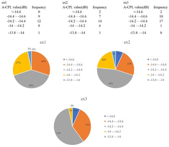
Figure 4.
Comparison of A-CPL frequency distribution under different experimental conditions.
The average running time of the three experiments is 430.82 s, 431.53 s, and 1202.87 s, respectively.
In summary, deploying the “individual uniqueness strategy” can improve the algorithm’s optimization results with negligible additional complexity. The comparison between ex3 and ex2 in Figure 3 and Figure 4 shows that the integration of IGCS can further improve the orthogonal performance of the ODCSs. However, the running time is nearly three times longer than ex1.
4.2. Design Results
Under constraints of , , , and weight coefficient , the optimized ODCSs by using MA-IGCS is shown in Table 2. After the autocorrelation function and cross-correlation function of the ODCSs in Table 2 are calculated, then the ASP and CP of the ODCSs are obtained according to (9) and (10). Table 3 shows the autocorrelation and cross-correlation properties of the ODCSs in Table 2.
Table 2.
The optimized ODCSs with L = 4, N = 40, M = 4, and weighting coefficient w = 0.5.
Table 3.
The autocorrelation and cross-correlation properties of ODCSs in Table 2.
The normalized autocorrelation sidelobe peak and cross-correlation peak levels of the designed ODCSs are shown in Table 3. The diagonal terms in Table 3 represent the ASPL of the optimized ODCSs and the off-diagonal terms are the CPL between two different sequences in the ODCSs. It can be observed that the data in Table 3 are diagonally symmetric, so it is sufficient to focus on either the upper triangular or lower triangular data. The A-ASPL and A-CPL are −19.37 dB and −14.23 dB, respectively.
To further illustrate the superiority of the optimization algorithm proposed in this paper, Table 4 lists the A-ASPL and A-CPL of the ODCSs with L = 4, N = 40, M = 4 designed by different optimization algorithms. The ODCSs optimized with the MA-IGCS are 0.47–2.87 dB lower than other optimization algorithms in A-ASPL. The MA-IGCS achieves an approximate performance as the MA-GCS concerning the A-CPL is 0.23–1.03 dB lower than the remaining optimization algorithms. In summary, it can be seen from Table 3 and Table 4 that compared with the existing optimization algorithms, the orthogonality of the ODCSs optimized with the MA-IGCS is further improved.
Table 4.
Comparison of A-ASPL and A-CPL values of ODCSs with L = 4, N = 40, M = 4 designed by different optimization algorithms.
4.3. Comparison with MA-GCS
Previously, we introduced various optimization algorithms and compared their design results with the MA-IGCS. In this part, we further compare the the ODCSs achieved by the MA-IGCS and MA-GCS in different conditions to demonstrate the superiority of the proposed algorithm. The comparison is limited to the MA-IGCS and MA-GCS because the code set generated by the MA-GCS exhibits the best observed orthogonal performance so far. The MA-GCS method is replicated according to the specific process given in reference [23], in which the partial restart method presented in the reference is not included. The particular implementation steps of the proposed MA-IGCS are shown in Algorithm 2, and the “individual uniqueness strategy” proposed in this paper does not apply to the MA-GCS.
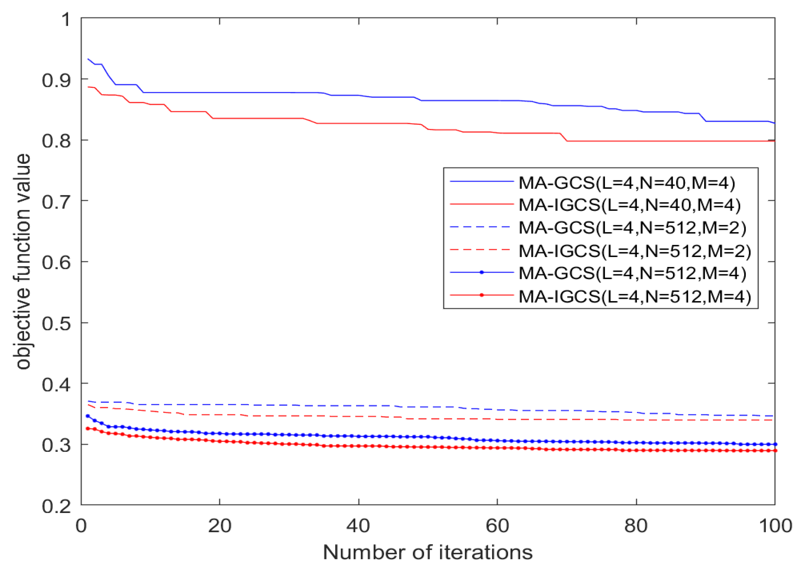
Figure 5 illustrates how the objective function value varies in each iteration under the three different conditions. It can be seen from Figure 5 that during each iteration with same parameters, the objective function value of the MA-IGCS is consistently lower than that of the MA-GCS. After the last iteration, compared to the MA-GCS, the MA-IGCS achieves a significant reduction in the objective function of the ODCSs. That shows that the MA-IGCS has more powerful search capabilities. Additionally, it can be inferred from Figure 5 that there is a significant decrease in the objective function values of the ODCSs when code length N increases from 40 to 512. Furthermore, when the number of optional phases is increased from 2 to 4, the objective function values of the ODCSs drop considerably as well.
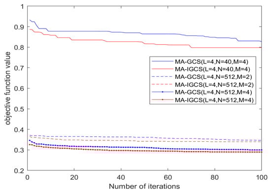
Figure 5.
Objective function value comparison between MA-IGCS and MA-GCCS.
Table 5 lists the results of ten simulation rounds with the parameter set of , , and to compare the MA-IGCS and MA-GCS in terms of objective function values, A-ASPL, and A-CPL. In this table, the objective function values obtained by the MA-IGCS vary from 0.81353 to 0.79795. All are less than the best objective function achieved by the MA-GCS. In the simulation results of the MA-GCS, the A-ASPL values range from −17.50445 to −18.54728, and the A-CPL values span from −14.06608 to −14.44138. The ODCSs optimized with the MA-GCS exhibits good cross-correlation properties, while its autocorrelation properties still need to be improved. Compared to the MA-GCS, the outcome of the MA-IGCS shows a substantial enhancement in the autocorrelation property and a modest improvement in the cross-correlation property.
Table 5.
Comparison of A-ASPL and A-CPL values of ODCSs with L = 4, N = 40, M = 4 designed by MA-IGCS and MA-GCS.
Table 6 further compares the A-ASPL and A-CPL of the optimized ODCSs with L = 4, N = 512, and M = 2 between the MA-IGCS and MA-GCS. The results suggest that the optimized ODCSs with MA-IGCS are consistently superior to the result obtained by the MA-GCS. Table 7 changes the number of optional phases from two to four in Table 6, which offers higher design freedom. Therefore, the A-CPL of the optimized ODCSs exhibits a great improvement compared to Table 6. Similar to Table 5 and Table 6, the results in Table 7 show that the ODCSs with , , and optimized by the MA-IGCS has better orthogonal performance. The above experimental results demonstrate that the MA-IGCS can obtain higher-quality solutions than state-of-the-art algorithms.
Table 6.
Comparison of A-ASPL and A-CPL values of ODCSs with L = 4, N = 512, M = 2 designed by MA-IGCS and MA-GCS.
Table 7.
Comparison of A-ASPL and A-CPL values of ODCSs with L = 4, N = 512, M = 4 designed by MA-IGCS and MA-GCS.
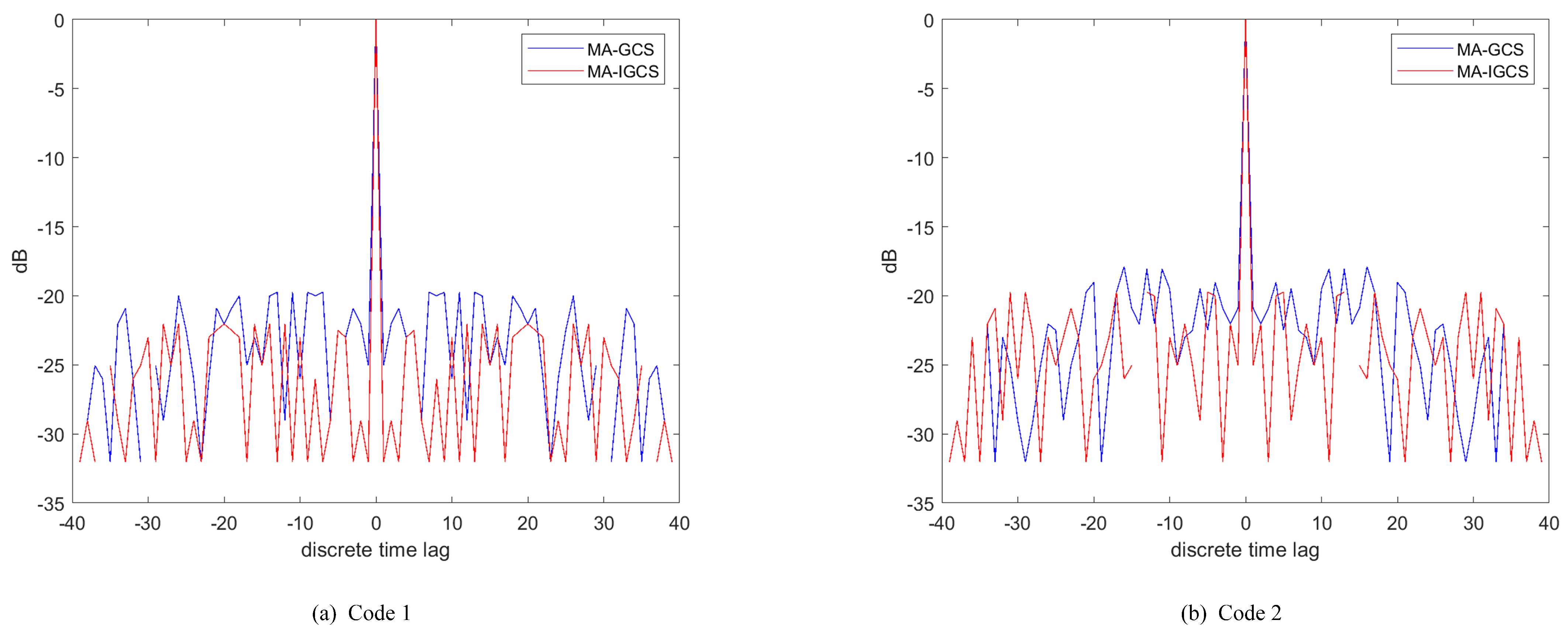
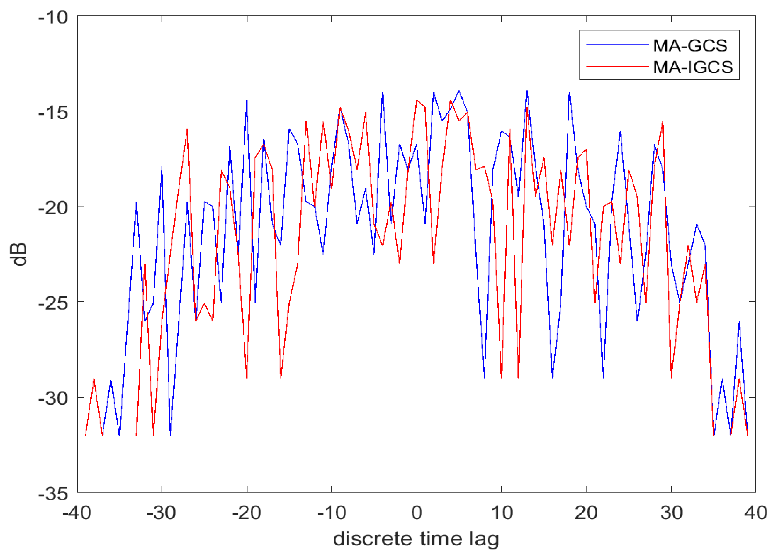
To demonstrate the performance of the MA-IGCS and MA-GCS more intuitively and not take up too much space, the autocorrelation and cross-correlation of the optimal four-phase code obtained by the two algorithms with , are depicted in Figure 6 and Figure 7, respectively. From Figure 6 and Figure 7, it can be inferred that the MA-IGCS algorithm achieves a lower autocorrelation sidelobe peak level than the MA-GCS algorithm, and the cross-correlation peak level is comparable.
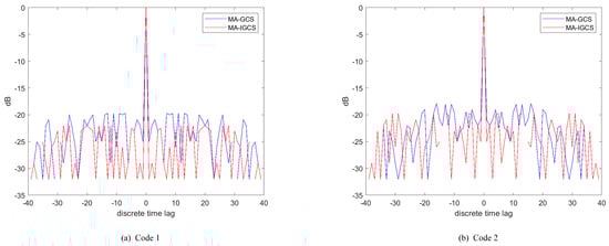
Figure 6.
Comparison of autocorrelation results for MA-IGCS and MA-GCS with L = 2, M = 4 and N = 40.
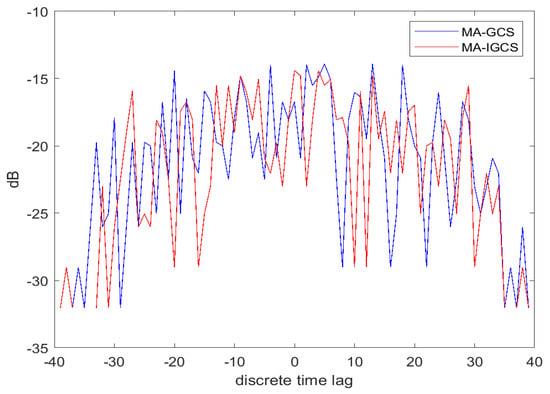
Figure 7.
Comparison of cross-correlation result for MA-IGCS and MA-GCS with L = 2, M = 4 and N = 40.
5. Conclusions
A novel and effective hybrid optimization algorithm, MA-IGCS, is proposed for optimizing the orthogonal waveform used in MIMO radar. This new algorithm chooses the MA as the algorithmic framework, IGCS as the local search approach, and incorporates an “individual uniqueness strategy” to maintain population diversity during iteration. We conducted three sets of comparative experiments to illustrate the benefits of integrating IGCS and the “individual uniqueness strategy” into the original algorithm framework. Based on the experimental results, it is clear that incorporating the “individual uniqueness strategy” can decrease the objective function value of optimized ODCSs without increasing execution runtime. Moreover, incorporating IGCS at the local search level further improves the orthogonality performance of the optimized ODCSs.
To show the effectiveness of the proposed algorithm, various ODCSs were designed with our algorithm under different conditions of code set sizes L, code length N, and optional phase numbers M. We first compared the A-ASPL and A-CPL of ODCSs designed by different optimization algorithms under constraints of L=4, N=40, and M=4, and the result shows that the MA-IGCS has best design results compared to other optimization algorithms. Furthermore, we conducted a comprehensive experimental comparison between the MA-IGCS and MA-GCS across different parameters. The analysis of simulation results indicates that the ODCSs designed by the proposed algorithm has better orthogonality than the state-of-the-art algorithm. Therefore, applying the ODCSs designed with the MA-IGCS to a CDMA-MIMO radar system can improve its signal detection capability and positioning accuracy. Although the MA-IGCS achieves better optimization results, a considerable gap remains between the designed ODCSs and the lower bound on peak sidelobe of Welch’s aperiodic correlation function. How to narrow this gap further is an important issue that needs to be fixed in the next stage.
Author Contributions
Conceptualization, W.W. and L.Q.; methodology, W.W.; validation, W.W. and L.Q.; formal analysis, W.W.; investigation, Y.Z.; data curation, W.W.; writing—original draft preparation, W.W.; writing—review and editing, L.Q. and Y.Z.; visualization, W.W.; supervision, L.Q. and Y.Z.; project administration, L.Q. and Y.Z.; funding acquisition, L.Q. and Y.Z. All authors have read and agreed to the published version of the manuscript.
Funding
This research was funded by the National Natural Science Foundation of China under Grant 42027805.
Data Availability Statement
The original contributions presented in the study are included in the article; further inquiries can be directed to the corresponding author.
Conflicts of Interest
The authors declare no conflicts of interest.
References
- Rabideau, D.J. Adaptive MIMO radar waveforms. In Proceedings of the 2008 IEEE Radar Conference, Rome, Italy, 26–30 May 2008; IEEE: Piscataway, NJ, USA, 2008; pp. 1–6. [Google Scholar]
- Sun, H.; Gao, C.; The, K.C. Performance evaluation of practical MIMO radar waveforms. In Proceedings of the 2016 IEEE Radar Conference (RadarConf), Philadelphia, PA, USA, 2–6 May 2016; IEEE: Piscataway, NJ, USA, 2016; pp. 1–6. [Google Scholar]
- Sun, H.; Brigui, F.; Lesturgie, M. Analysis and comparison of MIMO radar waveforms. In Proceedings of the 2014 International Radar Conference, Lille, France, 13–17 October 2014; IEEE: Piscataway, NJ, USA, 2014; pp. 1–6. [Google Scholar]
- Rambach, K.; Yang, B. MIMO radar: Time division multiplexing vs. code division multiplexing. In Proceedings of the International Conference on Radar Systems (Radar 2017), Belfast, UK, 23–26 October 2017; IET: Hertfordshire, UK, 2017; pp. 1–5. [Google Scholar]
- Mbeutcha, M.; Krozer, V. CDMA-based MIMO FMCW radar system performance using intra-pulse phase modulation. In Proceedings of the 2019 16th European Radar Conference (EuRAD), Paris, France, 2–4 October 2019; IEEE: Piscataway, NJ, USA, 2019; pp. 233–236. [Google Scholar]
- Solodky, G.; Longman, O.; Villeval, S.; Bilik, I. CDMA-MIMO Radar With the Tansec Waveform. IEEE Trans. Aerosp. Electron. Syst. 2021, 57, 76–89. [Google Scholar] [CrossRef]
- Baral, A.B.; Torlak, M. Joint Doppler frequency and direction of arrival estimation for TDM MIMO automotive radars. IEEE J. Sel. Top. Signal Process. 2021, 15, 980–995. [Google Scholar] [CrossRef]
- Cohen, D.; Cohen, D.; Eldar, Y.C. High Resolution FDMA MIMO Radar. IEEE Trans. Aerosp. Electron. Syst. 2020, 56, 2806–2822. [Google Scholar] [CrossRef]
- Sun, Y.; Bauduin, M.; Bourdoux, A. Enhancing unambiguous velocity in doppler-division multiplexing mimo radar. In Proceedings of the 2021 18th European Radar Conference (EuRAD), London, UK, 5–7 April 2022; IEEE: Piscataway, NJ, USA, 2022; pp. 493–496. [Google Scholar]
- Lian, H.; Lu, F.; Chen, Q.; Long, J.; Hu, X. DDMA-MIMO Radar Maximum Unambiguous Velocity Extension Based on Global Optimization Phase Modulation. In Proceedings of the 2021 CIE International Conference on Radar (Radar), Haikou, China, 15–19 December 2021; IEEE: Piscataway, NJ, USA, 2021; pp. 2856–2861. [Google Scholar]
- Deng, H. Polyphase code design for orthogonal netted radar systems. IEEE Trans. Signal Process. 2004, 52, 3126–3135. [Google Scholar] [CrossRef]
- Rajabi Moshtaghi, H.; Toloie Eshlaghy, A.; Motadel, M.R. A comprehensive review on meta-heuristic algorithms and their classification with novel approach. J. Appl. Res. Ind. Eng. 2021, 8, 63–89. [Google Scholar]
- Wang, Y.; Chen, M. A Novel MIMO Radar Orthogonal Waveform Design Algorithm Based on the Multi-Objective Improved Archimedes Optimization Algorithm. Remote Sens. 2023, 15, 5231. [Google Scholar] [CrossRef]
- Khan, H.; Edwards, D. Doppler problems in orthogonal MIMO radars. In Proceedings of the 2006 IEEE Conference on Radar, Verona, NY, USA, 24–27 April 2006; IEEE: Piscataway, NJ, USA, 2006; p. 4. [Google Scholar] [CrossRef]
- Sekiya, R.; Mori, H.; Hashimoto, H.; Suzuki, J. Design of Phase-Quantized Unimodular Waveforms on Neural Networks for MIMO Radar Systems. In Proceedings of the 2023 IEEE International Radar Conference (RADAR), Sydney, Australia, 6–10 November 2023; IEEE: Piscataway, NJ, USA, 2023; pp. 1–6. [Google Scholar]
- Sebdani, F.R.; Nasri, M. Binary Water Stream Algorithm: A New Metaheuristic Optimization Technique. In Proceedings of the 2023 14th International Conference on Information and Knowledge Technology (IKT), Isfahan, Iran, 26–28 December 2023; IEEE: Piscataway, NJ, USA, 2023; pp. 181–185. [Google Scholar]
- Hu, H.; Liu, B. Genetic algorithm for designing polyphase orthogonal code. In Proceedings of the 2008 4th International Conference on Wireless Communications, Networking and Mobile Computing, Dalian, China, 12–17 October 2008; IEEE: Piscataway, NJ, USA, 2008; pp. 1–4. [Google Scholar]
- Zeng, X.; Zhang, Y.; Guo, Y. Polyphase coded signal design for MIMO radar using MO-MicPSO. J. Syst. Eng. Electron. 2011, 22, 381–386. [Google Scholar] [CrossRef]
- Reddy, B.R.; M, U. Design of orthogonal waveform for MIMO radar using Modified Ant Colony Optimization Algorithm. In Proceedings of the 2014 International Conference on Advances in Computing, Communications and Informatics (ICACCI), Delhi, India, 24–27 September 2014; IEEE: Piscataway, NJ, USA, 2014; pp. 2554–2559. [Google Scholar]
- Reddy, B.R.; Uttarakumari, M. Optimization of discrete frequency coding waveform for MIMO radar using Modified Ant Colony Optimization algorithm. In Proceedings of the 2014 First International Conference on Networks & Soft Computing (ICNSC2014), Guntur, India, 19–20 August 2014; IEEE: Piscataway, NJ, USA, 2014; pp. 15–19. [Google Scholar]
- Liu, T.; Sun, J.; Wang, G.; Du, X.; Hu, W. Designing Low Side-Lobe Level-Phase Coded Waveforms for MIMO Radar Using P-Norm Optimization. IEEE Trans. Aerosp. Electron. Syst. 2023, 59, 3797–3810. [Google Scholar] [CrossRef]
- Liu, B.; He, Z.; Zeng, J.; Liu, B. Polyphase Orthogonal Code Design for MIMO Radar Systems. In Proceedings of the 2006 CIE International Conference on Radar, Shanghai, China, 16–19 October 2006; IEEE: Piscataway, NJ, USA, 2006; pp. 1–4. [Google Scholar]
- Ren, W.; Zhang, H.; Liu, Q.; Yang, Y. Greedy Code Search Based Memetic Algorithm for the Design of Orthogonal Polyphase Code Sets. IEEE Access 2019, 7, 13561–13576. [Google Scholar] [CrossRef]
- Huang, L.; Liu, A.; Gao, C. A Review of Orthogonal Waveform Design and Signal Processing in Colocated MIMO Radar. Radar Sci. Technol. 2023, 21, 1–15, 23. [Google Scholar]
- Zhang, L.; Wen, F. A Novel MIMO Radar Orthogonal Waveform Design Algorithm Based on Intelligent Ions Motion. Remote Sens. 2021, 13, 1968. [Google Scholar] [CrossRef]
- Katz, D.J.; van der Linden, C.M. Peak Sidelobe Level and Peak Crosscorrelation of Golay–Rudin–Shapiro Sequences. IEEE Trans. Inf. Theory 2022, 68, 3455–3473. [Google Scholar] [CrossRef]
- Liu, B.; He, Z.; Li, J. Mitigation of autocorrelation sidelobe peaks of orthogonal discrete frequency-coding waveform for MIMO radar. In Proceedings of the 2008 IEEE Radar Conference , Rome, Italy, 26–30 May 2008; IEEE: Piscataway, NJ, USA, 2008; pp. 1–6. [Google Scholar]
- Moscato, P. On evolution, search, optimization, genetic algorithms and martial arts: Towards memetic algorithms. Caltech Concurr. Comput. Program C3p Rep. 1989, 826, 37. [Google Scholar]
- Horng, S.C.; Lin, S.Y.; Lee, L.H.; Chen, C.H. Memetic Algorithm for Real-Time Combinatorial Stochastic Simulation Optimization Problems With Performance Analysis. IEEE Trans. Cybern. 2013, 43, 1495–1509. [Google Scholar] [CrossRef] [PubMed]
- Wang, B.; Shi, Q.; Mei, Q. Improvement of LS-SVM for time series prediction. In Proceedings of the 2014 11th International Conference on Service Systems and Service Management (ICSSSM), Beijing, China, 25–27 June 2014; IEEE: Piscataway, NJ, USA, 2014; pp. 1–5. [Google Scholar]
- Wang, N.; Wang, H.; Fu, Y.; Wang, D. A decomposition based memetic multi-objective algorithm for continuous multi-objective optimization problem. In Proceedings of the The 27th Chinese Control and Decision Conference (2015 CCDC), Qingdao, China, 23–25 May 2015; IEEE: Piscataway, NJ, USA, 2015; pp. 896–900. [Google Scholar]
- Zhuang, Z.; Fan, S.; Xu, H.; Zheng, J. A memetic algorithm using partial solutions for graph coloring problem. In Proceedings of the 2016 IEEE Congress on Evolutionary Computation (CEC), Vancouver, BC, Canada, 24–29 July 2016; IEEE: Piscataway, NJ, USA, 2016; pp. 3200–3206. [Google Scholar]
- Wang, B.g.; Zhang, G.h. Hybrid VNS and memetic algorithm for solving the job shop scheduling problem. In Proceedings of the 2011 IEEE 18th International Conference on Industrial Engineering and Engineering Management, Changchun, China, 3–5 September 2011; IEEE: Piscataway, NJ, USA, 2011; Volume 2, pp. 924–927. [Google Scholar]
- San-José-Revuelta, L.M. Design of Optimal Frequency-Selective FIR Filters Using a Memetic Algorithm. In Proceedings of the 2018 26th European Signal Processing Conference (EUSIPCO), Roma, Italy, 3–7 September 2018; IEEE: Piscataway, NJ, USA, 2018; pp. 1172–1176. [Google Scholar]
- Ahandani, M.A.; Baghmisheh, M.T.V. Memetic algorithms for solving university course timetabling problem. In Proceedings of the 2011 1st International eConference on Computer and Knowledge Engineering (ICCKE), Mashhad, Iran, 13–14 October 2011; IEEE: Piscataway, NJ, USA, 2011; pp. 40–44. [Google Scholar]
- Hart, W.E.; Krasnogor, N.; Smith, J.E. Recent Advances in Memetic Algorithms; Springer: Berlin/Heidelberg, Germany, 2005. [Google Scholar]
- Indiresan, P.; Uttaradhi, G. Iterative method for obtaining good aperiodic binary sequences. J. Optim. Theory Appl. 1971, 7, 90–108. [Google Scholar] [CrossRef]
- Singh, S.; Rao, K.S. Modified simulated annealing algorithm for poly phase code design. In Proceedings of the 2006 IEEE International Symposium on Industrial Electronics, Montreal, QC, Canada, 9–13 July 2006; IEEE: Piscataway, NJ, USA, 2006; Volume 4, pp. 2966–2971. [Google Scholar]
- Ramarakula, M.; Ramana, V. Optimization of Polyphase Orthogonal sequences for MIMO Radar Using Genetic Algorithm with Hamming Scan. In Proceedings of the 2019 IEEE International Conference on Advanced Networks and Telecommunications Systems (ANTS), Goa, India, 16–19 December 2019; IEEE: Piscataway, NJ, USA, 2019; pp. 1–5. [Google Scholar]
- Reddy, B.R.; Kumari, M.U. Polyphase orthogonal waveform using Modified Particle Swarm Optimization Algorithm for MIMO radar. In Proceedings of the 2012 IEEE International Conference on Signal Processing, Computing and Control, Solan, India, 15–17 March 2012; IEEE: Piscataway, NJ, USA, 2012; pp. 1–6. [Google Scholar]


Disclaimer/Publisher’s Note: The statements, opinions and data contained in all publications are solely those of the individual author(s) and contributor(s) and not of MDPI and/or the editor(s). MDPI and/or the editor(s) disclaim responsibility for any injury to people or property resulting from any ideas, methods, instructions or products referred to in the content. |
© 2025 by the authors. Licensee MDPI, Basel, Switzerland. This article is an open access article distributed under the terms and conditions of the Creative Commons Attribution (CC BY) license (https://creativecommons.org/licenses/by/4.0/).