Kinetic Energy Cascade in the Frequency Domain from Satellite Products

Abstract

Multiscale oceanic motions continuously transfer kinetic energy across various spatiotemporal scales through kinetic energy cascade. Satellite altimetry offers long-term daily ocean data at 0.25-degree resolution, enabling the analysis of energy cascades in both wavenumber and frequency domains. While energy cascade studies in the wavenumber domain are well-developed, frequency domain analyses remain limited. In this study, using 24 years of velocity data from satellite altimetry, we analyze the surface frequency-domain kinetic energy cascade primarily using the coarse-graining method. Compared to other approaches in literature, the coarse-graining approach shows superiority in diagnosing energy cascade in the frequency domain. Using this approach in the Kuroshio Extension region, we compare the spatiotemporal variability of energy cascades between the frequency and wavenumber domains. A pronounced low-frequency forward cascade, distinct from the wavenumber domain results, is identified. We propose a theory linking this low-frequency forward cascade with eddy generation through eddy–mean flow interactions. Significant variability is also observed in frequency domain energy cascades. Further analysis shows that wind forcing only plays a minor role in modulating the temporal variability of the energy cascade. Our findings are crucial for evaluating the model’s fidelity and advancing investigation of climate variability from the perspective of energy transfer.

1. Introduction

Oceanic motions, as part of a complex turbulent system, span a wide range of spatiotemporal scales. The kinetic energy (KE) within these motions is continually transferred across scales due to nonlinear interactions, which drives the ocean circulation system toward equilibrium. This process of cross-scale energy transfer, known as the energy cascade [1], serves as a crucial mechanism linking flows across vastly different scales [1,2,3]. An accurate estimation of the energy cascade is vital for understanding the ocean’s energy pathways and assessing its potential influence on low-frequency climate variability [4,5].

Rapid development of satellite altimetry in recent decades has brought unprecedented opportunities for geostrophic KE energy cascade study. Satellite altimetry offers daily data with a 0.25-degree resolution, enabling geostrophic KE cascade analyses in both the wavenumber and frequency domains. Based on the sea surface height (SSH) data from satellite altimetry, a predominant inverse KE cascade in the surface ocean was firstly observed in the wavenumber domain [2]. This inverse cascade, previously predicted by the two-dimensional quasi-geostrophic turbulence theory [1], demonstrates that geostrophic KE in the surface ocean predominantly transfers to larger spatial scales. Building on this pioneering work, significant progress has been made in the KE cascade study, especially using satellite altimetry data [6,7,8,9].

Current theories on KE energy cascade are primarily developed in the wavenumber domain. A commonly used metric for estimating KE transfer across different scales is the spectral KE flux. For gridded ocean data, three widely-used approaches for quantifying spectral KE fluxes in the wavenumber domain are: the spectral approach [8,10,11,12,13], the coarse-graining approach [5,14,15], and the method employed by Scott and Wang (hereafter the SW approach) [2,9,16]. Yang and Chen [17] systematically compared these three approaches in the wavenumber domain and highlighted the strengths of the coarse-graining approach for wavenumber domain KE cascade diagnosis, especially its adherence to Galilean invariance.

In contrast, diagnostic frameworks for frequency-domain KE cascades remain underdeveloped. Arbic et al. [6,18] proposed a stream-function-based spectral framework, which provides the first exploration of the frequency-domain KE cascade. They applied this framework to an idealized quasi-geostrophic (QG) model, a realistic ocean model, and satellite altimetry data. However, this spectral framework has two issues, which could potentially introduce biases in the frequency-domain KE cascade estimation: (i) it is essentially equivalent to the spectral approach, which includes a transport component according to Yang and Chen [17]; (ii) this spectral framework is derived based on a highly idealized two-layer QG model.

More recently, the coarse-graining approach [14] was extended to KE cascade studies in the frequency domain [19,20,21]. However, this approach has neither been applied to geostrophic KE cascade studies based on satellite altimetry, nor has it been used for low-frequency KE cascade analysis. Low-frequency KE cascade analysis is potentially critical for understanding climate variability. Previous studies mainly used in situ observations [20] or numerical simulations [19,20,21]. In addition, their focus is on high-frequency KE transfers, such as those within the submesoscale range [19,21] or between mesoscale and submesoscale ranges [20]. Despite these advancements, the two other approaches widely used in the wavenumber domain, the spectral approach and the SW approach, have not yet been extended to the frequency domain. In addition, systematic comparison among the three approaches in the frequency domain remain lacking. These methodological uncertainties would introduce potential biases into KE cascade studies. Given the limited evaluation of frequency domain KE cascade methods and their restricted application to satellite altimetry data across the whole available frequency ranges, we aim to (i) develop and compare various approaches for frequency domain KE cascades, and (ii) estimate KE cascades using satellite altimetry data at a wide range of frequencies.

Furthermore, the theoretical understanding of frequency domain energy cascades remains limited. From a spectral perspective, low wavenumbers are expected to correspond to low frequencies [22,23]. Inverse cascade has been typically identified at the low-wavenumber range [2,5,12]. Intuitively, one would expect that an inverse cascade would exist in the low-frequency range. However, using the spectral framework in the context of QG model, a strong forward cascade at low frequencies was previously identified by Arbic et al. [6] from the satellite altimetry data at some regions, such as the Kuroshio Extension region. Whether this phenomenon is sensitive to the choice of diagnostic approaches is to be determined. The mechanism for this low-frequency forward cascade also remains unclear. Therefore, another aim of this study is to investigate and interpret the underlying dynamics of this forward cascade in the low-frequency ranges. We also aim to systematically compare energy cascade in the frequency domain with that in the wavenumber domain, about which relatively few studies exist.

In this study, based on a 24-year velocity product of satellite altimetry from the Archiving, Validation, and Interpretation of Satellite Oceanographic Data (AVISO) program, we evaluate surface KE cascade in the frequency domain in the Kuroshio Extension region. As one of the most dynamically active areas in the global ocean, this region is characterized by intense multiscale interactions and contains a large portion of oceanic kinetic energy [11,24,25,26]. These features make this region an ideal site for KE cascade study.

KE cascade in this study is quantified through spectral KE fluxes. Comparison between three approaches highlights the superiority of the coarse-graining approach for KE cascade study in the frequency domain. Employing the coarse-graining approach, we compared the KE cascade results in the frequency and wavenumber domains. We observed a strong forward cascade at low frequencies, distinct from that in the wavenumber domain, and find that it is closely associated with eddy–mean flow interactions in this region. A theory linking low-frequency KE cascade and eddy–mean flow interaction is also proposed. Additionally, the temporal variability of KE cascades in the frequency domain differs from that in the wavenumber domain. Wind forcing is found to be a weak factor modulating the variability of KE cascades in the frequency domain.

This study is organized as follows. Section 2 introduces the definition of spectral KE energy flux and the three diagnostic methods in the frequency domain. Comparison between the three approaches in the frequency and wavenumber domains is also discussed. Section 3 describes the satellite products and data processing methods used in this study. Section 4 presents the main findings of this study. Section 5 is the summary and discussion.

2. Formulation of Diagnostic Framework

2.1. Definition of Kinetic Energy Cascade in the Frequency Domain

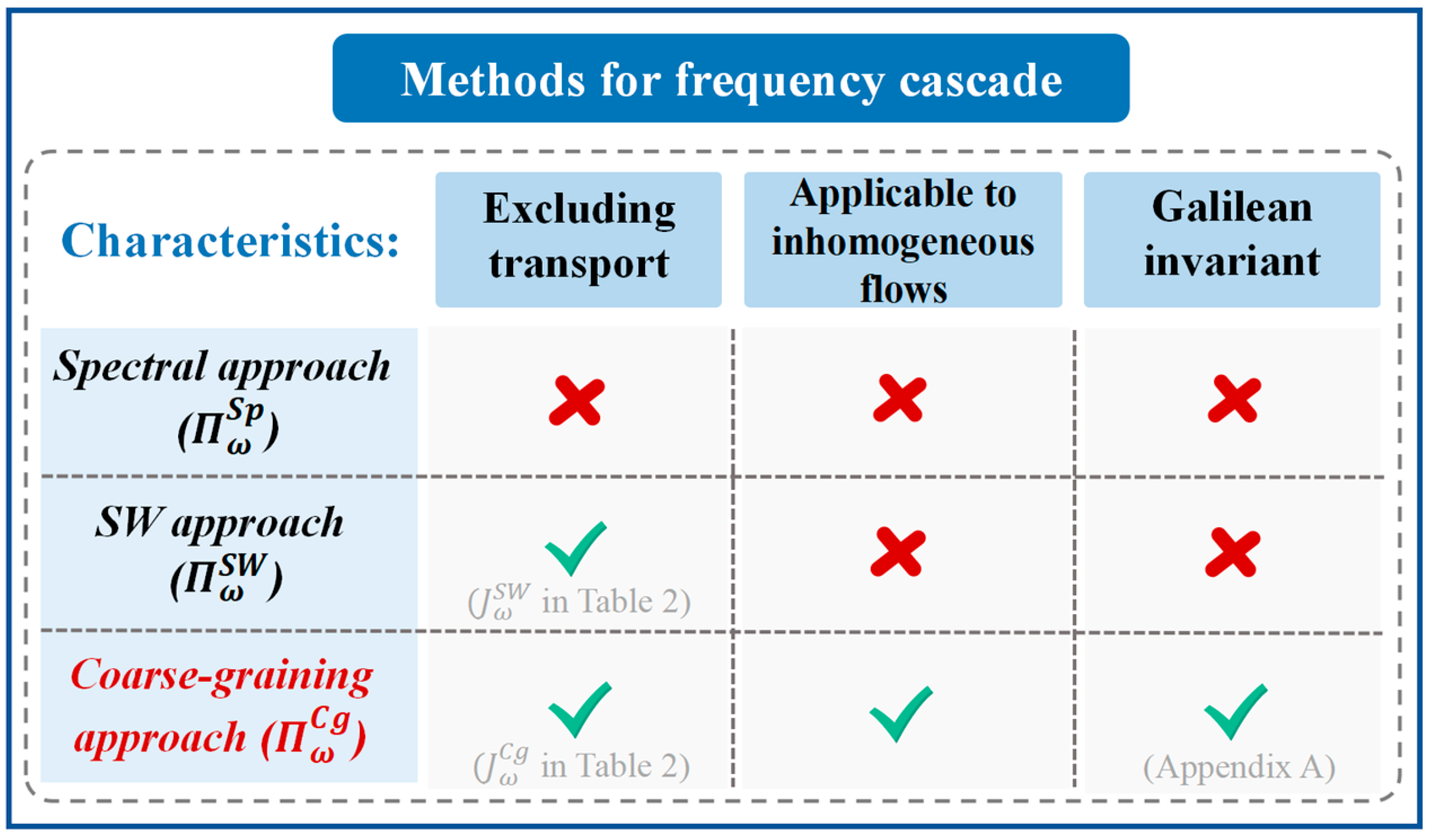
KE in the ocean is partitioned by different frequencies and generally increases quasi-monotonically with decreasing frequency [20,21,27] (Figure 1a). At low frequency, KE tends to vary slowly, while at high frequency, KE varies rapidly (Figure 1b). Due to the highly active coupling interaction between oceanic motions at different frequencies, KE constantly transfers across various frequencies through frequency KE cascade. Forward KE cascade in the frequency domain indicates KE transfer from low frequencies to high frequencies, while inverse KE cascade indicates transfer of KE from high frequencies to low frequencies (Figure 1b).

Spectral KE flux serves as a powerful metric for KE cascade study [2,15]. In the frequency domain, the spectral KE flux (${\Pi }_{\omega }$) quantifies KE transfer from flows at frequencies lower than a specific frequency $\omega$ to those at higher frequencies. A positive flux indicates a forward KE cascade, while a negative one indicates an inverse KE cascade. Through calculating ${\Pi }_{\omega }$ at each frequency, we can obtain the amounts of KE transfer across the whole available frequency range.

In this study, we introduce three definitions of spectral KE flux in the frequency domain: the spectral approach, the SW approach and the coarse-graining approach, which have proven effective for studying KE cascades in the wavenumber domain. Mathematical forms for these approaches are presented in

Table 1. Mathematical forms of the spectral KE flux in the three approaches. Refer to Supplementary Materials for detailed derivation.

Approach	Mathematical Form of Spectral KE Flux
$\mathrm{Spectral}\mathrm{approach}\left({\Pi }_{\omega }^{Sp}\right)$	${\Pi }_{\omega }^{Sp}={\displaystyle \sum _{\varpi >\omega }T(x,y,\varpi ) }\Delta \varpi ,$ where $T(x,y,\varpi )=-{\rho }_0\mathrm{Re} [\mathrm{F}{(u{\displaystyle \frac{\partial u}{\partial x}}+v{\displaystyle \frac{\partial u}{\partial y}})}_{\varpi }\mathrm{F}{(u)}_{\varpi }^{*}+\mathrm{F}{(u{\displaystyle \frac{\partial v}{\partial x}}+v{\displaystyle \frac{\partial v}{\partial y}})}_{\varpi }\mathrm{F}{(v)}_{\varpi }^{*}]$
$\mathrm{SW}\mathrm{approach}\left({\Pi }_{\omega }^{SW}\right)$	${\Pi }_{\omega }^{SW}={\rho }_0[u_{\omega }^{<}(u{\displaystyle \frac{\partial u_{\omega }^{>}}{\partial x}}+v{\displaystyle \frac{\partial u_{\omega }^{>}}{\partial y}})+v_{\omega }^{<}(u{\displaystyle \frac{\partial v_{\omega }^{>}}{\partial x}}+v{\displaystyle \frac{\partial v_{\omega }^{>}}{\partial y}})]$
$\mathrm{Coarse}-\mathrm{graining}\mathrm{approach}\left({\Pi }_{\omega }^{Cg}\right)$	${\Pi }_{\omega }^{Cg}=-{\rho }_0[{\tau }_{\omega }(u,u){\displaystyle \frac{\partial u_{\omega }^{<}}{\partial x}}+{\tau }_{\omega }(u,v)\left({\displaystyle \frac{\partial u_{\omega }^{<}}{\partial y}}\right.\left.+{\displaystyle \frac{\partial v_{\omega }^{<}}{\partial x}}\right)+{\tau }_{\omega }(v,v){\displaystyle \frac{\partial v_{\omega }^{<}}{\partial y}}],$ where ${\tau }_{\omega }(u_i,u_j)={(u_i{u}_j)}_{\omega }^{<}-u_{i\omega }^{<}{u}_{j\omega }^{<}$

Here, u is the zonal velocity and v is the meridional velocity. ${\cdot }_{\omega }^{<}$ and ${\cdot }_{\omega }^{>}$ represent the low-pass filtered and high-pass filtered components, respectively. ${\rho }_0$ is the seawater referenced density and takes a constant of 1027.4 kg m⁻³. $T(x,y,\varpi )$ in the spectral approach originates from the advection term in the momentum equation. It measures the redistribution of kinetic energy among different frequencies. $\varpi =2\pi n/T$ is the frequency at each sampling point, where $n\in \left[-N/2,N/2\right]$ and T is the total sampling duration. N is the total sampling points. $\mathrm{F}(\cdot )$ denotes taking the discrete Fourier transform (DFT) and * indicates complex conjugate. $\mathrm{Re}(\cdot )$ denotes taking the real part. The subfilter stress ${\tau }_{\omega }(u_i,u_j)$ in the coarse-graining approach represents the contribution of high-frequency flows at frequencies higher than $\omega$ to lower-frequency flows.

. For their detailed derivation, see S1 in Supplementary Materials. The three approaches introduced here have the following unique aspects:

• The spectral approach (${\Pi }_{\omega }^{Sp}$ in Table 1): The spectral approach here is developed directly from the primitive equations, instead of from the highly idealized quasi-geostrophic model as that in Arbic et al. [6,18]. It is essentially a natural extension of the spectral approach in the wavenumber domain [10,13] to the frequency domain. Based on the momentum equations (Equation (S1) and (S2) in Supplementary Materials), the spectral KE flux from this approach is obtained through the integration of Fourier-transformed advection term from one specific frequency to the highest available frequency;
• The SW approach (${\Pi }_{\omega }^{SW}$ in Table 1): The SW approach is developed for frequency-domain KE cascade for the first time. It is extended from the method proposed by Frisch [16] and Scott and Wang [2], which has not been applied in the frequency domain. Through applying a low-pass filter to momentum equations, this approach obtains spectral KE flux from the low-frequency KE budget equation. The low-pass filter here is defined as a specific type of filter that allows signals with a frequency lower than the cutoff frequency to pass through, while attenuating signals with frequencies higher than the cutoff frequency. The advection of low-frequency kinetic energy by total velocity ($J_{\omega }^{SW}$ in Table 2) is excluded from the original advection term due to its small effects to KE budget [16];
• The coarse-graining approach (${\Pi }_{\omega }^{Cg}$ in Table 1): Here, the coarse-graining approach is firstly applied to satellite altimetry data and shows its superiority in accurately estimating KE cascade. It was initially introduced by Aluie et al. [14], and was recently extend to the frequency domain [19,20,21] focusing on KE transfer at high frequencies. In situ observations [20] and numerical simulations [19,20,21] were used in these studies. However, previous literature [5,15,21] did not apply this approach to satellite altimetry-based study, and results of low-frequency KE cascade are also yet to be explored from this approach. Here, we apply the coarse-graining approach to the KE cascade study at the whole available frequency range, spanning from monthly to yearly timescales. The KE cascade term from the low-frequency KE budget equation is separated from a transport part ($J_{\omega }^{Cg}$ in Table 2).

2.2. Discussion: Comparison Among the Three Approaches

Here we compare the three approaches proposed in Section 2.1 in the frequency domain for the first time. In contrast with the other two approaches in Table 1 and Table 2, coarse-graining approach has three advantages: (i) the exclusion of transport component, (ii) applicability to inhomogeneous flows and (iii) adherence to Galilean invariance (Figure 2).

As shown in Figure 2, unlike the other two approaches, the coarse-graining approach does not rely on assumptions of homogeneity or isotropy [14,15,19,20], making it particularly effective for investigating energy transfer mechanisms in heterogeneous flow regimes. Additionally, both the coarse-graining approach and SW approach exclude a transport part (Table 2) from the KE cascade term, which only redistribute KE spatially but do not contribute to the KE transfer across different frequencies. Another unique advantage of the coarse-graining approach is its adherence to Galilean invariance (see proof in Appendix A). Galilean invariance ensures that cascade estimates remain invariant under inertial frame transformations, preventing errors caused by advective effects in methods that don’t have this property [14]. Such theoretical robustness provides superior quantification of KE transfer rates compared to the other two approaches.

To further confirm the advantages of the coarse-graining approach, we compared the spectral KE fluxes from the three approaches at the Kuroshio Extension region (Appendix B). Our numerical results again show that the coarse-graining approach is superior in accurately assessing KE cascade through excluding a transport part and adhering to Galilean invariance (Figure A1). For detailed information, refer to Appendix B and Figure A1.

Table 2. Mathematical forms of the transport terms in the SW and coarse-graining approaches. Refer to Supplementary Materials for detailed derivation.

Approach	Mathematical Form of Transport Term
SW approach	$J_{\omega }^{SW}={\rho }_0\left(u_{\omega }^{<}u{\displaystyle \frac{\partial u_{\omega }^{<}}{\partial x}}+u_{\omega }^{<}v{\displaystyle \frac{\partial u_{\omega }^{<}}{\partial y}}+v_{\omega }^{<}u{\displaystyle \frac{\partial v_{\omega }^{<}}{\partial x}}+v_{\omega }^{<}v{\displaystyle \frac{\partial v_{\omega }^{<}}{\partial y}}\right)$
Coarse-graining approach	$\begin{array}{cc}\hfill J_{\omega }^{Cg}& ={\displaystyle \frac{\partial }{\partial x}}(u_{\omega }^{<}\cdot K{E}_{\omega }^{<})+{\displaystyle \frac{\partial }{\partial y}}(v_{\omega }^{<}\cdot K{E}_{\omega }^{<})\hfill \\ & +{\rho }_0\left\{{\displaystyle \frac{\partial }{\partial x}}[u_{\omega }^{<}{\tau }_{\omega }(u,u)+v_{\omega }^{<}{\tau }_{\omega }(u,v)]+{\displaystyle \frac{\partial }{\partial y}}[u_{\omega }^{<}{\tau }_{\omega }(u,v)+v_{\omega }^{<}{\tau }_{\omega }(v,v)]\right\}\hfill \end{array}$

Here, $K{E}_{\omega }^{<}$ is defined as $K{E}_{\omega }^{<}={\displaystyle \frac{1}{2}}{\rho }_0(u_{\omega }^{<}{u}_{\omega }^{<}+v_{\omega }^{<}{v}_{\omega }^{<})$, which represents kinetic energy of low-frequency flows. $J_{\omega }^{SW}$ represents the advection of low-pass-filtered velocity with total velocity. $J_{\omega }^{Cg}$ represents transports of $K{E}_{\omega }^{<}$ due to low-frequency and high-frequency flows.

Table 2. Mathematical forms of the transport terms in the SW and coarse-graining approaches. Refer to Supplementary Materials for detailed derivation.

Approach	Mathematical Form of Transport Term
SW approach	$J_{\omega }^{SW}={\rho }_0\left(u_{\omega }^{<}u{\displaystyle \frac{\partial u_{\omega }^{<}}{\partial x}}+u_{\omega }^{<}v{\displaystyle \frac{\partial u_{\omega }^{<}}{\partial y}}+v_{\omega }^{<}u{\displaystyle \frac{\partial v_{\omega }^{<}}{\partial x}}+v_{\omega }^{<}v{\displaystyle \frac{\partial v_{\omega }^{<}}{\partial y}}\right)$
Coarse-graining approach	$\begin{array}{cc}\hfill J_{\omega }^{Cg}& ={\displaystyle \frac{\partial }{\partial x}}(u_{\omega }^{<}\cdot K{E}_{\omega }^{<})+{\displaystyle \frac{\partial }{\partial y}}(v_{\omega }^{<}\cdot K{E}_{\omega }^{<})\hfill \\ & +{\rho }_0\left\{{\displaystyle \frac{\partial }{\partial x}}[u_{\omega }^{<}{\tau }_{\omega }(u,u)+v_{\omega }^{<}{\tau }_{\omega }(u,v)]+{\displaystyle \frac{\partial }{\partial y}}[u_{\omega }^{<}{\tau }_{\omega }(u,v)+v_{\omega }^{<}{\tau }_{\omega }(v,v)]\right\}\hfill \end{array}$

Here, $K{E}_{\omega }^{<}$ is defined as $K{E}_{\omega }^{<}={\displaystyle \frac{1}{2}}{\rho }_0(u_{\omega }^{<}{u}_{\omega }^{<}+v_{\omega }^{<}{v}_{\omega }^{<})$, which represents kinetic energy of low-frequency flows. $J_{\omega }^{SW}$ represents the advection of low-pass-filtered velocity with total velocity. $J_{\omega }^{Cg}$ represents transports of $K{E}_{\omega }^{<}$ due to low-frequency and high-frequency flows.

2.3. Comparison Between Methods in the Frequency and Wavenumber Domains

One of the goals of this study is to compare energy cascade features from the frequency domain with those in the wavenumber domain. Therefore, for the convenience of the readers, here we also provide the mathematical forms of these approaches in the wavenumber domain (

Table 3. Mathematical forms of the three approaches in the wavenumber domain. These formulas are based on [17].

Approach	Mathematical Form of Spectral KE Flux
$\mathrm{Spectral}\mathrm{approach}\left({\Pi }_K^{Sp}\right)$	${\Pi }_K^{Sp}={\displaystyle \sum _{\kappa >K}T(k_x,k_y,t)}\Delta k^2,$ where $T(k_x,k_y,t)=-{\rho }_0\mathrm{Re}[\mathrm{F}{(u{\displaystyle \frac{\partial u}{\partial x}}+v{\displaystyle \frac{\partial u}{\partial y}})}_k\mathrm{F}{(u)}_k^{*}+\mathrm{F}{(u{\displaystyle \frac{\partial v}{\partial x}}+v{\displaystyle \frac{\partial v}{\partial y}})}_k\mathrm{F}{(v)}_k^{*}]$
$\mathrm{SW}\mathrm{approach}\left({\Pi }_K^{SW}\right)$	${\Pi }_K^{SW}={\rho }_0[u_K^{<}(u{\displaystyle \frac{\partial u_K^{>}}{\partial x}}+v{\displaystyle \frac{\partial u_K^{>}}{\partial y}})+v_K^{<}(u{\displaystyle \frac{\partial v_K^{>}}{\partial x}}+v{\displaystyle \frac{\partial v_K^{>}}{\partial y}})]$
$\mathrm{Coarse}-\mathrm{graining}\mathrm{approach}\left({\Pi }_K^{Cg}\right)$	${\Pi }_K^{Cg}=-{\rho }_0[{\tau }_K(u,u){\displaystyle \frac{\partial u_K^{<}}{\partial x}}+{\tau }_K(u,v)\left({\displaystyle \frac{\partial u_K^{<}}{\partial y}}\right.\left.+{\displaystyle \frac{\partial v_K^{<}}{\partial x}}\right)+{\tau }_K(v,v){\displaystyle \frac{\partial v_K^{<}}{\partial y}}],$ where ${\tau }_K(u_i,u_j)={(u_i{u}_j)}_K^{<}-u_{iK}^{<}{u}_{jK}^{<}$

Here, u and v are zonal and meridional velocities, respectively. $\left(k_x,k_y\right)=2\pi \left(m/L_x,n/L_y\right)$ is the horizontal wavenumber vector, where $m\in \left[-{\displaystyle \frac{N_x}{2}},{\displaystyle \frac{N_x}{2}}\right]$ and $n\in \left[-{\displaystyle \frac{N_y}{2}},{\displaystyle \frac{N_y}{2}}\right]$. $N_x$ and $N_y$ are grid point numbers in zonal and meridional directions, respectively. $L_x$ and $L_y$ are zonal and meridional domain sizes, respectively. $\kappa =\sqrt{k_x^2+k_y^2}$ is isotropic wavenumber. $\mathrm{F}(\cdot )$ denotes taking the discrete Fourier transform (DFT) and * indicates complex conjugate. $\mathrm{Re}(\cdot )$ denotes taking the real part. ${\cdot }_K^{<}$ and ${\cdot }_K^{>}$ represent the low-pass filtered and high-pass filtered components in the wavenumber domain, respectively. Detailed derivation of the three approaches can be found in [17].

). As shown in Table 1 and Table 3, the three methods share similar forms in both the frequency and wavenumber domains. However, they differ in their physical kernels. Here, the subscripts “$\omega$” or “K” represent KE transfer rate at a specific frequency or wavenumber. In the frequency domain, the three approaches calculate the spectral KE fluxes by decomposing the one-dimensional velocity time series into components at different frequencies. The spectral KE flux thus represents the KE transfer rate across different temporal scales. In contrast, in the wavenumber domain, the spectral KE fluxes represent the KE transfer rate across different spatial scales, obtained by decomposing the 2-dimensional velocity fields into multiple wavenumber components.

3. Data and Methods

3.1. Satellite Products

In this study, we utilize satellite altimetry data from AVISO to diagnose spectral KE fluxes. Previous studies have confirmed that the AVISO data is useful for energy cascade study [2,5,6,9]. To obtain energy cascade results for a wide range of frequencies, we choose to use the geostrophic surface current velocity data with the temporal duration of 24 years (1 January 1994–31 December 2017). This dataset, with a spatial resolution of 0.25° and a temporal resolution of one day, is consistent with the in situ drifter data, confirming its effectiveness and reliability [28]. This dataset is also used to calculate the current velocities in the wind power input term within the KE budget.

Version 3.1 of Cross-Calibrated Multi-Platform (CCMP V3.1) is used to calculate the wind power input in Section 4.4. This product provides six-hourly vector wind data, integrating ocean surface wind observations from various satellite microwave sensors with a background field derived from reanalysis. The dataset has a spatial resolution of 0.25° and also spans the period from 1 January 1994 to 31 December 2017 in this study.

3.2. Filtering Methods

In the frequency domain, a convolution-based low-pass filter is applied to the time series of velocity data at each frequency when evaluating KE cascade from the SW approach and the coarse-graining approach. For any time series of velocity u, the low-pass filtered velocity at frequencies lower than the cutoff frequency $\omega$ can be defined as:

$$u_{\omega }^{<}=G_{\omega }\ast u,$$

(1)

where * is a convolution and $G_{\omega }$ is the normalized kernel (window) function. The filter kernel we used here is a fourth-order Butterworth kernel [29,30,31], whose response function is:

$$H(\omega )={\displaystyle \frac{1}{\sqrt{1+{\left({\omega }_s/\omega \right)}^{2n}}}},$$

(2)

where n is the order of the filter, which is set as four in this study. ${\omega }_s$ is the sample frequency, which is 1 cpd here. Then, the high-pass filtered velocity $u_{\omega }^{>}$ is defined as:

$$u_{\omega }^{>}=u-u_{\omega }^{<},$$

(3)

which retains the information of velocity at frequencies higher than $\omega$. This spectrally sharp filter has proven effective in several energy cascade studies in the frequency domain [20,21].

Through applying this Butterworth filter to velocity data from AVISO satellite altimetry, we can directly isolate the low-frequency and high-frequency component of the velocities. The spectral KE fluxes and spatial transports are then calculated using the formulas in Table 1 and Table 2. To mitigate the edge effects introduced by the filtering procedure [19,21], we truncated approximately 1.2 times the filter’s temporal scale from both ends of the filtered time series. For the spectral approach, inspired by the filtering method used in the wavenumber domain [8,12,17], we apply a discrete Fourier transform (DFT) operation to the velocity data to decompose scales in the frequency domain.

While in the wavenumber domain, to calculate ${\Pi }_K^{Cg}$ from the coarse-graining approach (Table 3), we use a uniform filter that has been widely used in literature [14,21,32] to decompose scales in the spatial space. The filter kernel is chosen to be a spatially sharp top-hat kernel [14,21,32].

3.3. Analysis

We estimate the KE cascade in the frequency domain over a range of frequencies from 5.48 × 10⁻⁴ cpd (cycles per day) to 0.01 cpd, corresponding to temporal scales of 5 years to 3 months. The minimum temporal scale of 3 months is determined based on the Nyquist period of satellite observations. Considering the periods discarded during the filtering process, the maximum temporal scale is set to 5 years, ensuring that half of the time series length (12 years) is retained for further analysis.

4. Results

Using satellite altimetry data, we characterize the kinetic energy cascade in the frequency domain at the Kuroshio Extension region. Given the established superiority of the coarse-graining approach in the wavenumber domain [5,14,15,17], we compare the KE cascade results in both the frequency and wavenumber domains using this approach, aiming to fully elucidate the underlying mechanisms of the frequency-domain KE cascades in the Kuroshio Extension region. The spatiotemporal variability of KE cascades in both the wavenumber and frequency domains is also compared. We found that compared to the results in the wavenumber domain, KE cascade in the frequency domain is characterized by a strong forward cascade at low frequencies (mostly at frequencies lower than 0.002 cpd). This is closely associated with eddy–mean flow interactions, through which energy can be exchanged between time-varying eddies and the mean flow (Section 4.1). We further propose a theory to support this finding (Appendix C). The inverse cascade in the frequency domain is generally stronger than that in the wavenumber domain (Section 4.2). Additionally, we demonstrate that the temporal variability of KE cascade in the frequency domain is weakly linked with wind forcing (Section 4.4).

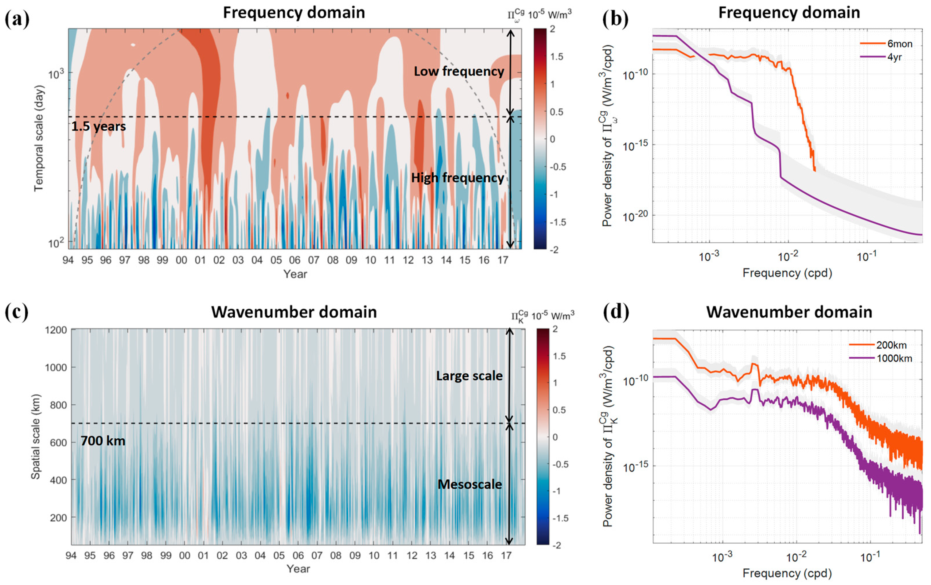
4.1. Forward Energy Cascades: Frequency vs. Wavenumber Domain Results

4.1.1. Phenomenon

Unlike the predominant upscale KE transfer observed in wavenumber space [2,5,8,12,14] (Figure 3a), the frequency-domain KE cascade in the Kuroshio Extension region is characterized by a strong downscale transfer, particularly at very low frequencies (Figure 3b). This low-frequency forward cascade was also noted by Arbic et al. [6] using AVISO satellite altimetry data. However, the mechanism of the low-frequency forward cascade has not been considered in literature. This is partially because this phenomenon seems counterintuitive: Low-wavenumber motions generally have low-frequencies [22,23] and thus inverse cascade at low wavenumbers should correspond to inverse cascade at low frequencies; however, forward cascade at low frequencies have been identified here. The discrepancy between the wavenumber-domain and frequency-domain KE cascade results in the Kuroshio Extension region reveals the complex relationship between temporal and spatial scales in this region.

We define the maximum positive value of a spectral kinetic energy flux as the amplitude of the forward kinetic energy cascade (hereafter Amp_forward), which quantifies the strength of forward cascade. The spatial pattern for Amp_forward in the frequency domain reveals that the frequency domain forward cascade predominantly occurs in the Kuroshio Extension region (Figure 3c), with approximately 83% of the grid points displaying forward cascading behavior. Strong forward cascades are predominantly observed in the upstream of the Kuroshio Extension region, particularly in areas where the jet flow is intense. Considering the distinctions between the forward cascades in the frequency and wavenumber domains, we next explore the underlying mechanism of the low-frequency forward cascade from the perspective of eddy–mean flow interactions.

4.1.2. Interpretation

Eddy–mean flow interaction denotes the interaction between time–mean flow and time-varying eddies. Based on the eddy-driven theories, eddies can cause the mean flow to evolve, and the instabilities in the mean flow can generate eddies [33]. In this process, kinetic energy can be exchanged between eddies and mean flow [34,35]. This eddy–mean kinetic energy exchange process can be quantified by $M_{KE}$ in the ocean Lorenz energy cycle, which represents the eddy kinetic energy (EKE) change rate due to eddy momentum fluxes [34,36,37,38]. Its mathematical formula is

$$M_{KE}=-{\rho }_0[\overline{u^{\prime }{u}^{\prime }}{\displaystyle \frac{\partial \overline{u}}{\partial x}}+\overline{u^{\prime }{v}^{\prime }}\left({\displaystyle \frac{\partial \overline{u}}{\partial y}}\right.\left.+{\displaystyle \frac{\partial \overline{v}}{\partial x}}\right)+\overline{v^{\prime }{v}^{\prime }}{\displaystyle \frac{\partial \overline{v}}{\partial y}}],$$

(4)

where $\overline{\cdot }$ denotes mean flow, and $\cdot ’$ denotes the time-varying eddies. Note that $M_{KE}$ in this study is diagnosed using geostrophic velocity from satellite altimetry, which represents the contribution of geostrophic flow to $M_{KE}$ [34]. The eddy–mean kinetic energy exchange process, quantified by $M_{KE}$, is particularly prevalent in the Kuroshio Extension region. In the western part of the Kuroshio Extension, where barotropic instability is strong, most of the KE released from the mean flow tends to transfer to time-varying eddies (i.e., $M_{KE}$ > 0). In the eastern part, however, KE could be transferred back to the mean flow (i.e., $M_{KE}$ < 0) [34].

The linkage between low-frequency forward cascade and eddy–mean flow interaction can be rigorously derived through Fourier expansion (see Appendix C). In the Lorenz energy cycle, mean flow is typically defined as the time–mean flow, while eddies represent the time-varying motions. From the Fourier expansion of current velocity, it follows that zero-frequency flows correspond to the mean flow, while the flow component at non-zero frequencies represent time-varying eddies. Therefore, eddy–mean energy exchange through eddy–mean flow interaction directly corresponds to energy cascade at zero frequency (see detailed derivation in Appendix C). Specifically, a zero-frequency forward cascade (${\Pi }_0^{Cg}$ > 0) reflects the transfer of KE from the mean flow to eddies ($M_{KE}$ > 0), while a zero-frequency inverse cascade (${\Pi }_0^{Cg}$ < 0) indicates energy transferring back to the mean flow ($M_{KE}$ < 0). Therefore, it can be inferred that as long as the mean flow in a region is barotropically unstable, the low-frequency forward kinetic energy cascade will occur.

The numerical results from AVISO satellite altimetry data further validate the linkage between energy cascade at low frequencies and eddy–mean flow interaction process (Figure 4). Here we compare the time mean of ${\Pi }_{4yr}^{Cg}$, which is the spectral KE flux at the frequency of cycle/4 years, with eddy–mean energy exchange term $M_{KE}$. The spatial patterns for the spectral KE flux at other low frequencies (e.g., periods form 2 years to 5 years) are analogous to that of ${\Pi }_{4yr}^{Cg}$. Therefore, we choose the temporal scale of 4 years as a representative scale for low frequencies.

The spatial distributions of ${\Pi }_{4yr}^{Cg}$ and $M_{KE}$ are similar at the Kuroshio Extension region (Figure 4). Both ${\Pi }_{4yr}^{Cg}$ and $M_{KE}$ are characterized by large positive values in the western part of Kuroshio Extension, indicating forward cascade at low frequencies and eddy generation (Figure 4a,b,

Table 4. Spatiotemporal-averaged ${\Pi }_{4yr}^{Cg}$ and $M_{KE}$ at the Kuroshio Extension region estimated from satellite altimetric data. The western and eastern parts of the Kuroshio Extension are defined in Figure 4.

	Kuroshio Extension	Western Part	Eastern Part
$M_{KE}$(10−6 W/m3)	8.36	17.27	0.87
${\Pi }_{4yr}^{Cg}$(10−6 W/m3)	6.40	11.81	0.99

). In contrast, in the eastern part of the Kuroshio Extension, both ${\Pi }_{4yr}^{Cg}$ and $M_{KE}$ have magnitudes smaller than one (Table 4), and both spatial structures have positive and negative patches (Figure 4a,b). The probability density functions (PDF) of ${\Pi }_{4yr}^{Cg}$ and $M_{KE}$ also exhibit a similar pattern, both peaking at zero (Figure 4c). The PDF corresponding to the positive range of ${\Pi }_{4yr}^{Cg}$ and $M_{KE}$ is generally higher than that corresponding to the negative range, which indicates that the spatial distribution of ${\Pi }_{4yr}^{Cg}$ and $M_{KE}$ is predominantly dominated by positive values. The correlation coefficient between ${\Pi }_{4yr}^{Cg}$ and $M_{KE}$ reaches 0.90 ± 0.02, significant above the 95% confidence level. This further confirms the strong relationship between ${\Pi }_{4yr}^{Cg}$ and $M_{KE}$.

Table 4 reveals that the eddy–mean flow interaction in the entire Kuroshio Extension region is predominantly governed by eddy generation (the spatiotemporal-averaged $M_{KE}$ is 8.36 × 10⁻⁶ W/m³), where KE transfers from mean flow to eddies. This is closely associated with the strong low-frequency forward cascade in this region.

4.2. Inverse Energy Cascades: Frequency vs. Wavenumber Domain Results

Analogous to the amplitude of forward cascade, the amplitude of inverse KE cascade (hereafter Amp_inverse) is defined as the minimum negative value of a spectral KE flux (Figure 5), which represents the strength of the inverse energy cascade’s strength. As shown in Figure 5, inverse cascades in the frequency domain primarily occur at medium frequencies (monthly timescales) that are considerably higher than zero frequency (Figure 5a). As a result, they cannot be attributed to eddy–mean flow interaction. Instead, the medium-frequency inverse cascades are analogous to those in the medium-wavenumber range (Figure 5b). In the wavenumber domain, inverse cascades strengthen as wavenumbers approach the mesoscale range. Considering the broad continuum of motions across all spatiotemporal scales [22,23], the spatial mesoscale range can be roughly associated with the temporal medium range. This implies that regions with more mesoscale activities are likely to experience stronger inverse cascades in the frequency domain. This can be further supported by the similarity between the spatial patterns for Amp_inverse in the frequency and wavenumber domains, with both showing higher concentrations in regions of elevated kinetic energy levels (Figure 5c,d).

Nevertheless, a noticeable difference in Amp_inverse between the frequency and wavenumber domains is observed in the Kuroshio Extension region (Figure 5e,f). The spatial pattern of the difference in Amp_inverse indicates that inverse cascades are generally more pronounced in the frequency domain compared to those in the wavenumber domain, particularly in regions with intense currents. In contrast, in coastal areas, inverse cascades in the wavenumber domain tend to be stronger (Figure 5e). The PDF of the difference in Amp_inverse further illustrates the dominance of stronger inverse cascades in the frequency domain, with the PDF in the negative range being higher than that in the positive range.

4.3. Temporal Variability of Energy Cascade: Frequency vs. Wavenumber Domain Results

In the frequency domain, low-frequency KE cascades tend to exhibit variability over long temporal scales, whereas high-frequency cascades fluctuate on shorter temporal scales (Figure 6a). To investigate the temporal variability of frequency-domain KE cascades, we calculate regional averages of spectral fluxes and analyze the time series of the spectral flux at each frequency we consider. The results indicate that the temporal variability of energy cascades depends on the scale (or frequency): spectral KE fluxes at larger temporal scales evolve more slowly, while those at smaller temporal scales fluctuate faster. In addition, the KE cascades at larger temporal scales (or lower frequencies) tend to be stronger. As the temporal scale increases, forward cascades grow in strength and become more dominant in the Kuroshio Extension region. This behavior is closely linked to the eddy generation process within eddy–mean flow interactions, as discussed in Section 4.1. The frequency spectra of the spectral KE flux at the two temporal scales further confirm our findings (Figure 6b). The peak frequencies for the two spectra are approximately 0.035 cpd for the 6-month scale and ~0 cpd for the 4-year scale. This indicates that the dominant frequencies at which KE cascades evolve in the frequency domain align with the frequency ranges of the cascades themselves.

In contrast, in the wavenumber domain, the temporal variability of KE cascades at different spatial scales is similar (Figure 6c). All the spectral KE fluxes exhibit rapid fluctuations. The frequency spectra of the spectral KE flux at spatial scales of 200 km (corresponding to the mesoscale range) and 1000 km (corresponding to the large-scale range) show similar tendencies, with values increasing as the frequency decreases (Figure 6d). However, the magnitude of KE cascades between the large-scale and mesoscale ranges differs significantly. Inverse cascades tend to be stronger in the mesoscale range (Figure 6c). The power density of spectral flux at the 200 km spatial scale is also consistently higher than that at the 1000 km scale across all available frequencies (Figure 6d). This suggests that in the wavenumber domain, the strength of KE cascades, rather than their temporal variability, tends to vary with spatial scales.

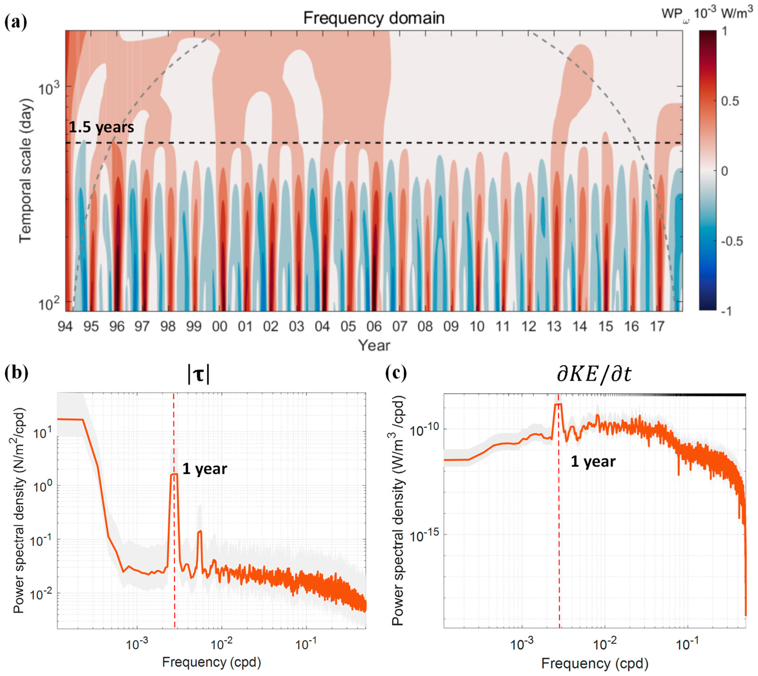
4.4. Linkage Between KE Cascades in the Frequency Domain and Wind Forcing

In this section, we investigate potential factors influencing the temporal variability of KE cascade in the frequency domain. On a global scale, O’Rourke et al. [39] discussed the potential relation between wind stress and KE cascade through the transfers of KE in the frequency domain. They quantified the relative contributions of wind forcing and intrinsic advection to low-frequency KE and identified a relative balance between the two, especially in regions with rich eddies. Consequently, they speculated that the KE cascade and wind forcing may be weakly linked. Inspired by their work, we evaluate the linkage between KE cascades and wind power input both at annual and other frequencies.

We define the wind power input term from the low-frequency KE budget as:

$$W{P}_{\omega }={\displaystyle \frac{u_{\omega }^{<}{\left({\tau }_x\right)}_{\omega }^{<}+v_{\omega }^{<}{\left({\tau }_y\right)}_{\omega }^{<}}{H}},$$

(5)

where ${\left({\tau }_x\right)}_{\omega }^{<}$ and ${\left({\tau }_y\right)}_{\omega }^{<}$ represent the low-pass filtered zonal and meridional surface wind stress at the frequency $\omega$, respectively. The wind stress here is estimated using the wind speeds based on the method in [32]. H is approximately the Ekman layer thickness, which is set as 10 m in this study [1]. $W{P}_{\omega }$ represents wind power input into low-frequency KE. See detailed derivation of $W{P}_{\omega }$ and the low-frequency KE budget in Supplementary Materials.

The temporal variability of $W{P}_{\omega }$ exhibits similarities to that of KE cascades in the frequency domain (Figure 7a). In the low-frequency range, $W{P}_{\omega }$ evolves gradually, while in the high-frequency range, it fluctuates rapidly (Figure 7a). The frequency spectra of $W{P}_{\omega }$ also show a similar trend to that of ${\Pi }_{\omega }^{Cg}$, with the peak frequency for the 6-month scale exceeding that for the 4-year scale. This further indicates that wind power input at higher (lower) frequencies tends to vary over shorter (longer) temporal scales.

A significant annual cycle, which is absent in the frequency-domain KE cascade variations (Figure 6a,b), exists in $W{P}_{\omega }$, particularly within the high-frequency band (Figure 7a). Consistently, the frequency spectrum of wind stress peaks at annual frequency (Figure 7b). A similar annual peak is also observed in the frequency spectra of geostrophic KE (Figure 1a) [39] and KE tendency term (Figure 7b). This indicates that the seasonal cycles of KE could be attributed more to the seasonal cycle of wind than to that of frequency-domain energy cascade. In the wavenumber domain, such a consistent and significant annual peak of wind and KE is absent.

Statistical analysis between $W{P}_{\omega }$ and ${\Pi }_{\omega }^{Cg}$ reveals that wind forcing is only weakly linked with KE cascade variations (

Table 5. Linkage between the KE cascades in the frequency domain (${\Pi }_{\omega }^{Cg}$) and wind power input term ($W{P}_{\omega }$) at the Kuroshio Extension region. The low-frequency (high-frequency) range corresponds to frequencies lower (higher) than one cycle per 1.5 years. A low-frequency (high-frequency) time series is derived by averaging all the fluxes in the low-frequency (high-frequency) range. The symbol “√” indicates significant correlation coefficients or information flow at the 95% confidence level.

${\mathsf{\Pi }}_{\mathit{\omega }}^{\mathit{C}\mathit{g}}$$\mathbf{and}\mathit{W}{\mathit{P}}_{\mathit{\omega }}$	Low Frequency		High Frequency
	With Annual Cycle	Without Annual Cycle	With Annual Cycle	Without Annual Cycle
Correlation coefficients	0.09 ± 0.03 [√]	0.09 ± 0.03 [√]	0.05 ± 0.02 [√]	0.07 ± 0.02 [√]
$\mathrm{Normalized}\mathrm{information}\mathrm{flow}\mathrm{from}W{P}_{\omega }$$\mathrm{to}{\Pi }_{\omega }^{Cg}$	0.02 ± 0.06	0.02 ± 0.06	0.07 ± 0.03 [√]	0.04 ± 0.04

). In both the low- and high-frequency ranges, $W{P}_{\omega }$ and ${\Pi }_{\omega }^{Cg}$ exhibit weak yet statistically significant correlations, with both the correlation coefficients reaching below 0.1. Considering that correlation does not imply causality [40], we also conducted a causality analysis [40,41]. The normalized information flow from $W{P}_{\omega }$ to ${\Pi }_{\omega }^{Cg}$ is significant in the high-frequency range (0.07 ± 0.02) but remains insignificant in the low-frequency range (0.02 ± 0.06). However, the information flow from $W{P}_{\omega }$ to ${\Pi }_{\omega }^{Cg}$ at both low- and high-frequencies becomes insignificant when excluding the annual cycle. This suggests that the wind variability significantly affects the frequency-domain cascade variability mainly at the annual frequency. Compared to wind, intrinsic nonlinear interaction itself plays a more significant role in modulating the variability of ${\Pi }_{\omega }^{Cg}$.

5. Conclusions and Discussion

In this study, using the velocity product from satellite altimetry data, we confirmed the superiority of the coarse-graining approach in the frequency-domain KE cascade study compared to the other two approaches. This is the first time that the coarse-graining approach is applied to the frequency-domain KE cascade diagnosis using satellite altimetry data. We also developed the spectral approach and the SW approach for the KE cascade diagnosis in the frequency domain. Here, for the first time, the SW approach is extended from the wavenumber domain to the frequency domain. The spectral approach for the frequency KE cascade diagnosis is also firstly derived based on the primitive equations.

Using the coarse-graining approach, we further compared the spatiotemporal variability of KE cascades in both the frequency and wavenumber domains at the Kuroshio Extension region. The usage of this method enables a more accurate estimation of energy cascade and validates the energy cascade results derived in this study. Unlike the predominant inverse cascades in the wavenumber domain, we identified a strong forward cascade at low frequencies and found that this phenomenon is closely associated with eddy generation during eddy–mean flow interactions. A theory linking low-frequency forward cascade with eddy–mean flow interaction is also proposed. In terms of the inverse cascade, the inverse KE cascades in the frequency domain are generally stronger than those in the wavenumber domain. Additionally, we observed distinct temporal variabilities of KE cascades in the frequency and wavenumber domains. The temporal variability of KE cascades in the frequency domain is found to be weakly influenced by wind forcing. This suggests that the intrinsic oceanic variability or other factors—such as the vertical transport or eddy diffusion which are not considered due to the lack of observational data—may contribute to the observed variations in the frequency domain KE cascade. Considering the potential errors in the velocity product [28], the errors in the spectral KE flux in this study are estimated to be approximately 30% based on error propagation. A further detailed calibration of our results is needed for future work.

A comparison between the results from our datasets and the latest satellite data reveals that our key conclusions are robust and insensitive to the choice of time period or the dataset we used. The velocity data used in this study is from the delayed-time altimetry product provided by the Multi-satellite Data Unification and Altimeter Combination System (DUACS DT2018), which was released in 2018 and includes current velocity data up until 2018. To assess the potential impact of the selected time range, we recalculated the main results using the recently updated DT2024 dataset, spanning from 1 January 1993 to 31 December 2023. We found that our key conclusions are not significantly affected by the choice of time period or dataset. Further analysis of the KE cascade using this updated product is planned for future work.

Previous studies have decomposed kinetic energy cascades in the wavenumber domain into normal strain and shear strain components [17,21]. However, Srinivasan et al. [21] demonstrated that this decomposition is sensitive to the rotation of the coordinate system and therefore lacks independent interpretability. They instead decomposed the kinetic energy cascade into rotational and divergent components, demonstrating that both components are coordinate-invariant. Further exploration is thus needed to extend this strain/divergence decomposition of energy cascade into the frequency domain. Other possible future work includes: (i) applying the diagnostic framework in this study, especially the coarse-graining approach, to other ocean regions; (ii) examining frequency domain kinetic energy cascades induced by ageostrophic motions; (iii) assessing the fidelity of ocean models and reanalysis data in representing geostrophic KE cascades; (iv) exploring the role of other factors, such as vertical transport of eddy diffusion, in modulating the temporal variability of KE cascades.

Our findings offer important insights. Firstly, we rigorously demonstrated the superiority of the coarse-graining approach. This approach will serve as an effective tool for evaluating the fidelity of model simulations in representing energy transfer across different spatiotemporal scales. The energy cascade results diagnosed from satellite altimetry can also provide a valuable baseline for assessing model fidelity. Secondly, the close relation between low-frequency forward cascade and eddy–mean flow interaction could help interpret multiscale KE transfer at low frequencies. Finally, our findings in the variability of the low-frequency cascade would potentially provide insights into investigation for climate variability from the energy transfer perspective.

References

1. Vallis, G.K. Atmospheric and Oceanic Fluid Dynamics, 1st ed.; Cambridge University Press: New York, NY, USA, 2006; p. 995. [Google Scholar]
2. Scott, R.B.; Wang, F. Direct evidence of an oceanic inverse kinetic energy cascade from satellite altimetry. J. Phys. Oceanogr. 2005, 35, 1650–1666. [Google Scholar] [CrossRef]
3. Alexakis, A.; Biferale, L. Cascades and transitions in turbulent flows. Phys. Rep. 2018, 767, 1–101. [Google Scholar] [CrossRef]
4. Sérazin, G.; Penduff, T.; Barnier, B.; Molines, J.-M.; Arbic, B.K.; Müller, M.; Terray, L. Inverse cascades of kinetic energy as a source of intrinsic variability: A global OGCM study. J. Phys. Oceanogr. 2018, 48, 1385–1408. [Google Scholar] [CrossRef]
5. Storer, B.A.; Buzzicotti, M.; Khatri, H.; Griffies, S.M.; Aluie, H. Global cascade of kinetic energy in the ocean and the atmospheric imprint. Sci. Adv. 2023, 9, eadi7420. [Google Scholar] [CrossRef]
6. Arbic, B.K.; Müller, M.; Richman, J.G.; Shriver, J.F.; Morten, A.J.; Scott, R.B.; Sérazin, G.; Penduff, T. Geostrophic turbulence in the frequency–wavenumber domain: Eddy-driven low-frequency variability. J. Phys. Oceanogr. 2014, 44, 2050–2069. [Google Scholar] [CrossRef]
7. Arbic, B.K.; Polzin, K.L.; Scott, R.B.; Richman, J.G.; Shriver, J.F. On eddy viscosity, energy cascades, and the horizontal resolution of gridded satellite altimeter products. J. Phys. Oceanogr. 2013, 43, 283–300. [Google Scholar] [CrossRef]
8. Wang, S.; Liu, Z.; Pang, C. Geographical distribution and anisotropy of the inverse kinetic energy cascade, and its role in the eddy equilibrium processes. J. Geophys. Res. Oceans 2015, 120, 4891–4906. [Google Scholar] [CrossRef]
9. Khatri, H.; Sukhatme, J.; Kumar, A.; Verma, M.K. Surface ocean enstrophy, kinetic energy fluxes, and spectra from satellite altimetry. J. Geophys. Res. Oceans 2018, 123, 3875–3892. [Google Scholar] [CrossRef]
10. Capet, X.; McWilliams, J.C.; Molemaker, M.J.; Shchepetkin, A.F. Mesoscale to submesoscale transition in the California Current System. Part III: Energy balance and flux. J. Phys. Oceanogr. 2008, 38, 2256–2269. [Google Scholar] [CrossRef]
11. Dong, J.; Fox-Kemper, B.; Zhang, H.; Dong, C. The seasonality of submesoscale energy production, content, and cascade. Geophys. Res. Lett. 2020, 47, e2020GL087388. [Google Scholar] [CrossRef]
12. Li, H.; Xu, Y. Barotropic and baroclinic inverse kinetic energy cascade in the Antarctic Circumpolar Current. J. Phys. Oceanogr. 2021, 51, 809–824. [Google Scholar] [CrossRef]
13. Qiu, B.; Scott, R.B.; Chen, S. Length scales of eddy generation and nonlinear evolution of the seasonally modulated South Pacific Subtropical Countercurrent. J. Phys. Oceanogr. 2008, 38, 1515–1528. [Google Scholar] [CrossRef]
14. Aluie, H.; Hecht, M.W.; Maltrud, M.E.; Rai, S.; Sadek, M.; Storer, B.A.; Vallis, G.K. Mapping the energy cascade in the North Atlantic Ocean: The coarse-graining approach. J. Phys. Oceanogr. 2018, 48, 225–244. [Google Scholar] [CrossRef]
15. Schubert, R.; Gula, J.; Greatbatch, R.J.; Baschek, B.; Biastoch, A. The submesoscale kinetic energy cascade: Mesoscale absorption of submesoscale mixed layer eddies and frontal downscale fluxes. J. Phys. Oceanogr. 2020, 50, 2573–2589. [Google Scholar] [CrossRef]
16. Frisch, U. Turbulence: The Legacy of A. N. Kolmogorov; Cambridge University Press: New York, NY, USA, 1995; p. 296. [Google Scholar]
17. Yang, Y.; Chen, R. Spectral kinetic-energy fluxes in the North Pacific: Definition comparison and normal- and shear-strain decomposition. J. Mar. Sci. Eng. 2022, 10, 1148. [Google Scholar] [CrossRef]
18. Arbic, B.K.; Scott, R.B.; Flierl, G.R.; Morten, A.J.; Richman, J.G.; Shriver, J.F. Nonlinear cascades of surface oceanic geostrophic kinetic energy in the frequency domain. J. Phys. Oceanogr. 2012, 42, 1577–1600. [Google Scholar] [CrossRef]
19. Barkan, R.; Srinivasan, K.; Yang, L.; McWilliams, J.C.; Gula, J.; Vic, C. Oceanic mesoscale eddy depletion catalyzed by internal waves. Geophys. Res. Lett. 2021, 48, e2021GL094376. [Google Scholar] [CrossRef]
20. Garabato, A.C.N.; Yu, X.; Callies, J.; Barkan, R.; Polzin, K.L.; Frajka-Williams, E.E.; Buckingham, C.E.; Griffies, S.M. Kinetic energy transfers between mesoscale and submesoscale motions in the open ocean’s upper layers. J. Phys. Oceanogr. 2022, 52, 75–97. [Google Scholar] [CrossRef]
21. Srinivasan, K.; Barkan, R.; McWilliams, J.C. A forward energy flux at submesoscales driven by fontogenesis. J. Phys. Oceanogr. 2023, 53, 287–305. [Google Scholar] [CrossRef]
22. Wortham, C.; Wunsch, C. A multidimensional spectral description of ocean variability. J. Phys. Oceanogr. 2014, 44, 944–966. [Google Scholar] [CrossRef]
23. Wunsch, C. The oceanic variability spectrum and transport trends. Atmosphere-Ocean 2009, 47, 281–291. [Google Scholar] [CrossRef]
24. Yang, H.; Qiu, B.; Chang, P.; Wu, L.; Wang, S.; Chen, Z.; Yang, Y. Decadal variability of eddy characteristics and energetics in the Kuroshio Extension: Unstable versus stable states. J. Geophys. Res. Oceans 2018, 123, 6653–6669. [Google Scholar] [CrossRef]
25. Cao, H.; Fox-Kemper, B.; Jing, Z. Submesoscale eddies in the upper ocean of the Kuroshio Extension from high-resolution simulation: Energy budget. J. Phys. Oceanogr. 2021, 51, 2181–2201. [Google Scholar] [CrossRef]
26. Chen, R.; Gille, S.T.; McClean, J.L. Isopycnal eddy mixing across the Kuroshio Extension: Stable versus unstable states in an eddying model. J. Geophys. Res. Oceans 2017, 122, 4329–4345. [Google Scholar] [CrossRef]
27. Martin, P.E.; Arbic, B.K.; Hogg, A.M.; Kiss, A.E.; Munroe, J.R.; Blundell, J.R. Frequency-domain analysis of the energy budget in an idealized coupled ocean–atmosphere model. J. Clim. 2020, 33, 707–726. [Google Scholar] [CrossRef]
28. Taburet, G.; Sanchez-Roman, A.; Ballarotta, M.; Pujol, M.I.; Legeais, J.F.; Fournier, F.; Faugere, Y.; Dibarboure, G. DUACS DT2018: 25 years of reprocessed sea level altimetry products. Ocean Sci. 2019, 15, 1207–1224. [Google Scholar] [CrossRef]
29. Butterworth, S. On the theory of filter amplifiers. Wirel. Eng. 1930, 7, 536–541. [Google Scholar]
30. Manal, K.; Rose, W. A general solution for the time delay introduced by a low-pass Butterworth digital filter: An application to musculoskeletal modeling. J. Biomech. 2007, 40, 678–681. [Google Scholar] [CrossRef]
31. Shouran, M.; Elgamli, E. Design and implementation of Butterworth filter. Int. J. Innov. Res. Sci. Eng. Technol. 2020, 9, 7975–7983. [Google Scholar]
32. Rai, S.; Hecht, M.; Maltrud, M.; Aluie, H. Scale of oceanic eddy killing by wind from global satellite observations. Sci. Adv. 2021, 7, eabf4920. [Google Scholar] [CrossRef]
33. Cronin, M. Eddy-mean flow interaction in the Gulf Stream at 68 W. Part II: Eddy forcing on the time-mean flow. J. Phys. Oceanogr. 1996, 26, 2132–2151. [Google Scholar] [CrossRef]
34. Chen, R.; Flierl, G.R.; Wunsch, C. A description of local and nonlocal eddy–mean flow interaction in a global eddy-permitting state estimate. J. Phys. Oceanogr. 2014, 44, 2336–2352. [Google Scholar] [CrossRef]
35. Kang, D.; Curchitser, E.N. Energetics of eddy–mean flow interactions in the Gulf Stream region. J. Phys. Oceanogr. 2015, 45, 1103–1120. [Google Scholar] [CrossRef]
36. Chen, R.; Yang, Y.; Geng, Q.; Stewart, A.; Flierl, G.; Wang, J. Diagnostic framework linking eddy flux ellipse with eddy-mean energy exchange. Ocean-Land-Atmos. Res. 2024, 3, olar.0072. [Google Scholar] [CrossRef]
37. Storch, J.-S.V.; Eden, C.; Fast, I.; Haak, H.; Hernández-Deckers, D.; Maier-Reimer, E.; Marotzke, J.; Stammer, D. An estimate of the Lorenz energy cycle for the world ocean based on the STORM/NCEP Simulation. J. Phys. Oceanogr. 2012, 42, 2185–2205. [Google Scholar] [CrossRef]
38. Waterman, S.; Jayne, S.R. Eddy-mean flow interactions in the along-stream development of a western boundary current jet: An idealized model study. J. Phys. Oceanogr. 2011, 41, 682–707. [Google Scholar] [CrossRef]
39. O’Rourke, A.K.; Arbic, B.K.; Griffies, S.M. Frequency-domain analysis of atmospherically forced versus intrinsic ocean surface kinetic energy variability in GFDL’s CM2-O model hierarchy. J. Clim. 2018, 31, 1789–1810. [Google Scholar] [CrossRef]
40. Liang, X.S. Unraveling the cause-effect relation between time series. Phys. Rev. E 2014, 90, 052150. [Google Scholar] [CrossRef]
41. Liang, X.S. Normalizing the causality between time series. Phys. Rev. E 2015, 92, 022126. [Google Scholar] [CrossRef]
42. Yang, H.; Chang, P.; Qiu, B.; Zhang, Q.; Wu, L.; Chen, Z.; Wang, H. Mesoscale air–sea interaction and its role in eddy energy dissipation in the Kuroshio Extension. J. Clim. 2019, 32, 8659–8676. [Google Scholar] [CrossRef]
Figure 1. Definition of kinetic energy cascade in the frequency domain. (a) Frequency spectrum of domain-averaged geostrophic kinetic energy from velocity product of satellite altimetry data at the Kuroshio Extension region. The red vertical dashed line indicates the frequency of 1/365 cycles per day (cpd), which marks the evident annual cycle of geostrophic KE in this region. (b) Schematic diagram of kinetic energy cascade in the frequency domain. Here the geostrophic KE at frequencies lower than frequency ω is defined as K E ω = 1 2 ρ 0 ( u ω 2 + v ω 2 ) , where u and v are zonal and meridional velocities, respectively. ρ 0 is referenced density and takes a constant of 1027.4 kg m−3. u ω and v ω are derived from low-pass-filtered velocities at (36°N, 142°E) based on gridded AVISO satellite altimetry. The red (blue) arrows represent the forward (inverse) cascades in the frequency domain.
Remotesensing 17 00877 g001
Figure 2. Schematic diagram illustrating the advantages and disadvantages of the three methods for diagnosing frequency-domain KE cascade. The term “excluding transport” refers to the exclusion of the spatial transport term, which does not represent energy cascade ( J ω S W and J ω C g in Table 2), from the spectral kinetic energy flux. “Applicable to inhomogeneous flows” allows the approach free of the assumption of homogeneity or isotropy. “Galilean invariant” refers to the property ensuring that cascade estimates remain invariant under inertial frame transformations. Approaches that align with the characteristics are marked with “√”, while those do not are marked with “×”.
Remotesensing 17 00877 g002
Figure 3. Comparison between the forward KE cascades in the wavenumber and frequency domain. (a) Spatiotemporal-averaged spectral kinetic energy flux in the wavenumber domain at the Kuroshio extension region. The diagnostic method used here is the coarse-graining approach in Table 3. (b) as in (a), but in the frequency domain. The vertical dashed grey line in (b) indicates the frequency at 0.01 cpd, and the solid red dot represents the amplitude of the forward cascade. Both of the two fluxes are estimated using AVISO satellite altimetry data. (c) Spatial pattern for forward cascade amplitude (Ampforward), which is defined in (b), in the frequency domain. A 1° running average is applied to the spatial map here. Gray lines in (c) indicate barotropic streamlines ψ = g η ¯ / f , where g is the gravitational acceleration, f is the Coriolis parameter, and η ¯ is the time–mean sea surface height.
Remotesensing 17 00877 g003
Figure 4. Relation between (a) low-frequency (at temporal scale of 4 years) kinetic energy transfer ( Π 4 y r C g ) and (b) eddy–mean energy exchange ( M K E ). Both Π 4 y r C g and M K E are calculated as a time mean from 1994–2017 using the velocity product of satellite altimetry data. The vertical dashed black lines at 150 °E in (a) and (b) divide the Kuroshio Extension region into western and eastern parts. A 2° running average is applied to the spatial maps here. (c) Probability density functions (PDF) of Π 4 y r C g and M K E . PDF represents the distribution of values for a given variable. (d) Grid point by grid point comparison between Π 4 y r C g and M K E . The correlation coefficient between them is 0.90 ± 0.02, which is significant above the 95% confidence level.
Remotesensing 17 00877 g004
Figure 5. Comparison between the inverse KE cascades in the wavenumber and frequency domain. (a) Time–mean spectral kinetic energy flux at (30°N, 132°E) in the frequency domain based on coarse-graining approach. The vertical dashed grey line indicates the frequency at 0.01 cpd. (b) as in (a), but in the wavenumber domain. The amplitude of inverse cascade (Ampinverse) is defined in (a) and (b). (c) Spatial pattern for Ampinverse in the frequency domain at the Kuroshio Extension region. (d) as in (c), but in the wavenumber domain. (e) Spatial pattern for difference in Ampinverse between the frequency domain and wavenumber domain (i.e., difference between (c) and (d)). Gray lines in (c), (d), and (e) indicate barotropic streamlines, which are defined in Figure 3. A 2° running average is applied to the spatial maps here. (f) Probability density function (PDF) of the difference in Ampinverse between the frequency domain and wavenumber domain.
Remotesensing 17 00877 g005
Figure 6. Temporal variability of KE cascade in the frequency and wavenumber domains at the Kuroshio Extension region. (a) Time series of regionally averaged spectral KE fluxes in the frequency domain at different temporal scales. The dashed grey lines represent the time boundaries of edge effects caused by the temporal filtering procedure. Our analysis focuses solely on the time series between the two boundaries. The dashed black line represents the temporal scale of 1.5 years. Frequencies lower than cycles/1.5 years (corresponding to temporal scales longer than 1.5 years) are defined as the low-frequency range, while frequencies higher than cycles/1.5 years (corresponding to temporal scales shorter than 1.5 years) are considered the high-frequency range. Here, only the spectral fluxes at temporal scales larger than 3 months are considered. (b) Frequency spectra of spectral KE flux at two representative temporal scales: 4 years for the low-frequency range and 6 months for the high-frequency range. (c) as in (a), but for spectral KE fluxes in the wavenumber domain at different spatial scales. The dashed black line represents the spatial scale of 700 km, which divides the entire spatial scale range into large-scale and mesoscale ranges. (d) Frequency spectra of spectral KE flux at two representative spatial scales: 1000 km for the large-scale range and 200 km for the mesoscale range. The grey shading in (b) and (d) indicates 95% confidence intervals. The estimated error in the spectral KE fluxes here is approximately 30% based on error propagation.
Remotesensing 17 00877 g006
Figure 7. Temporal variability of low-frequency wind power input term W P ω at the Kuroshio Extension region. (a) Time series of regionally averaged low-frequency wind power input W P ω at different temporal scales. The dashed grey lines and the dashed black line have the same meaning as those in Figure 6a. Only the fluxes for wind power input at temporal scales larger than 3 months are considered. (b) Frequency spectrum of the magnitude of wind stress ( τ = τ x 2 + τ y 2 ). The vertical dashed red line indicates the frequency at 1/365 cpd. (c) As in (b), but for KE tendency term ( K E / t ). The grey shading indicates 95% confidence intervals. Here, the wind stress is estimated using the wind speeds from CCMP V3.1.
Remotesensing 17 00877 g007