
A Cross-Track Interferometric Synthetic Aperture 3D Passive Positioning Algorithm

 , ,
, ,
Abstract
:
1. Introduction
2. Model and Methods
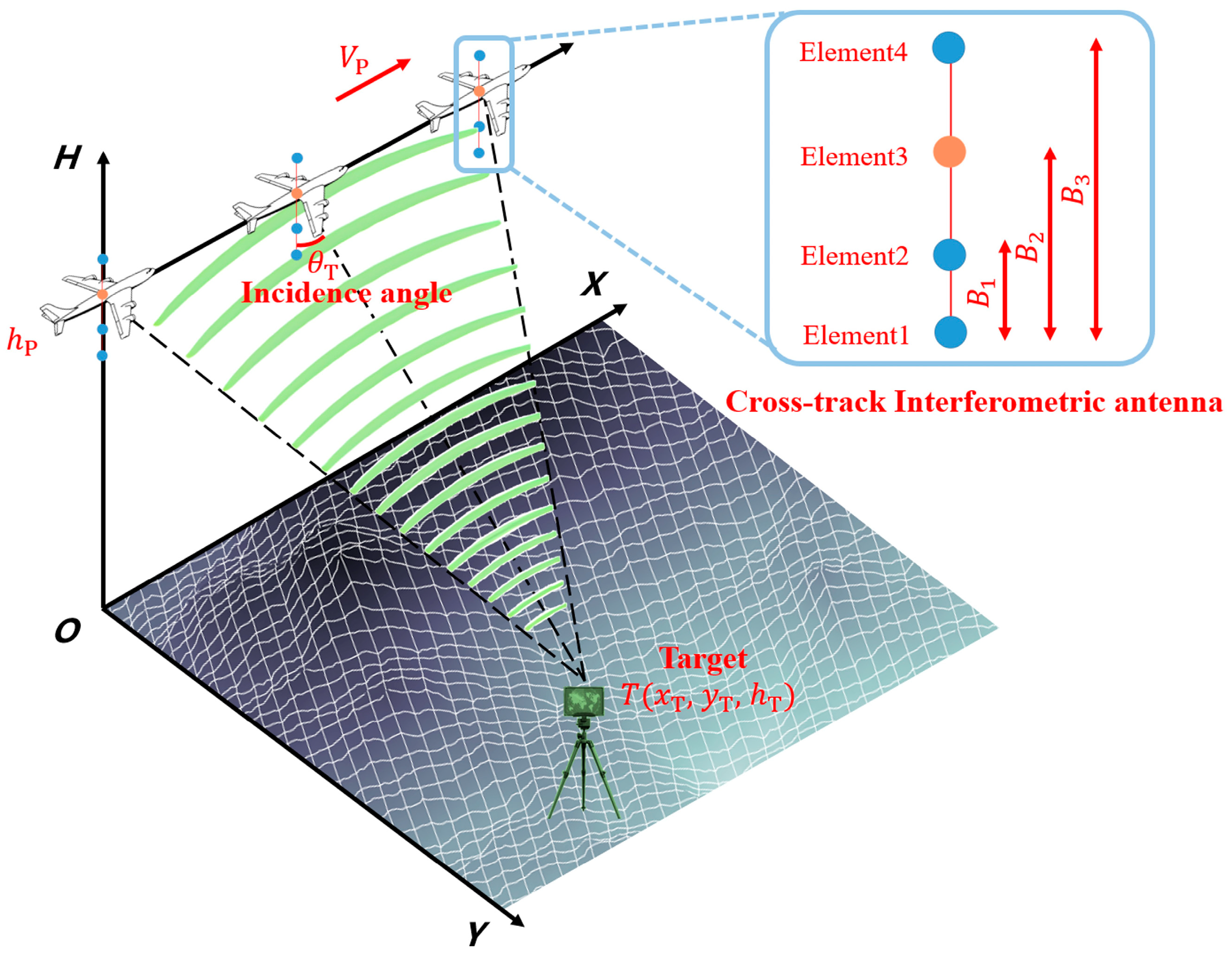
2.1. Signal Modeling
2.2. Cross-Track Interferometric Synthetic Aperture 3D Passive Positioning Algorithm
- (1)
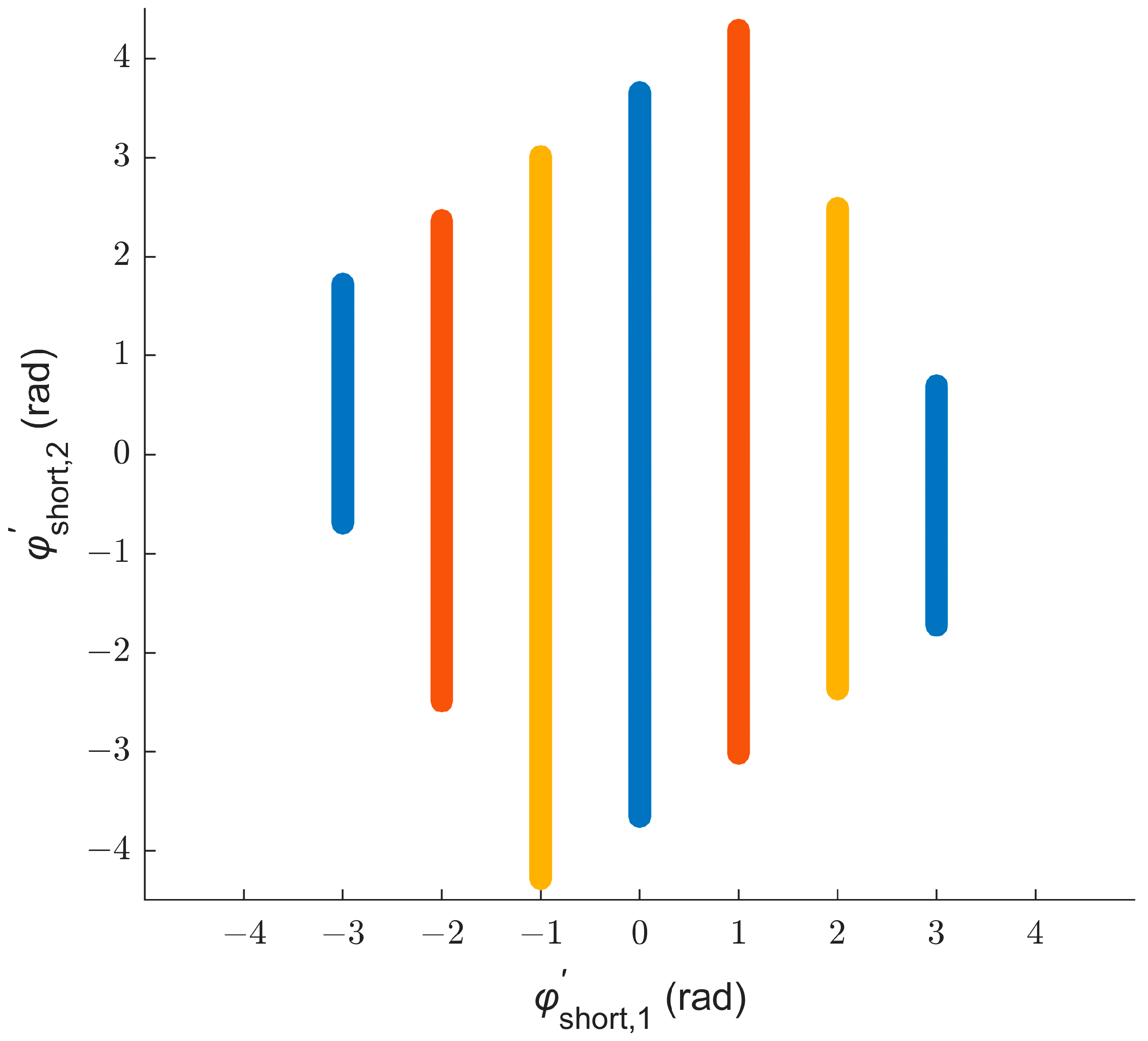
- Second-order differencing of the baselines yields two virtual short baselines and ;
- (2)
- The virtual baselines are prime multiples of the half-wavelength;
- (3)
- The prime numbers are as small as possible.
2.3. Effects of Incoherence on SAPP
3. Results
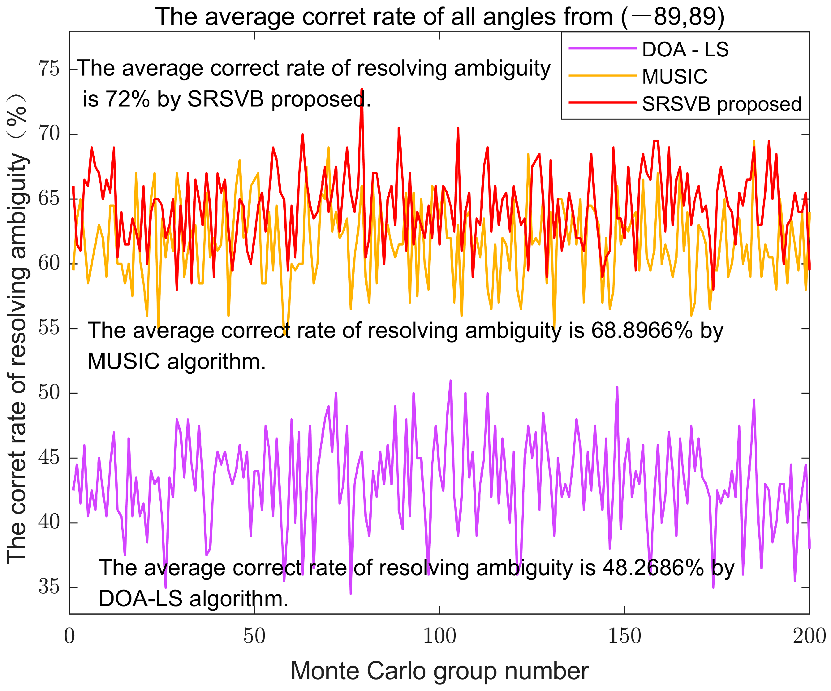
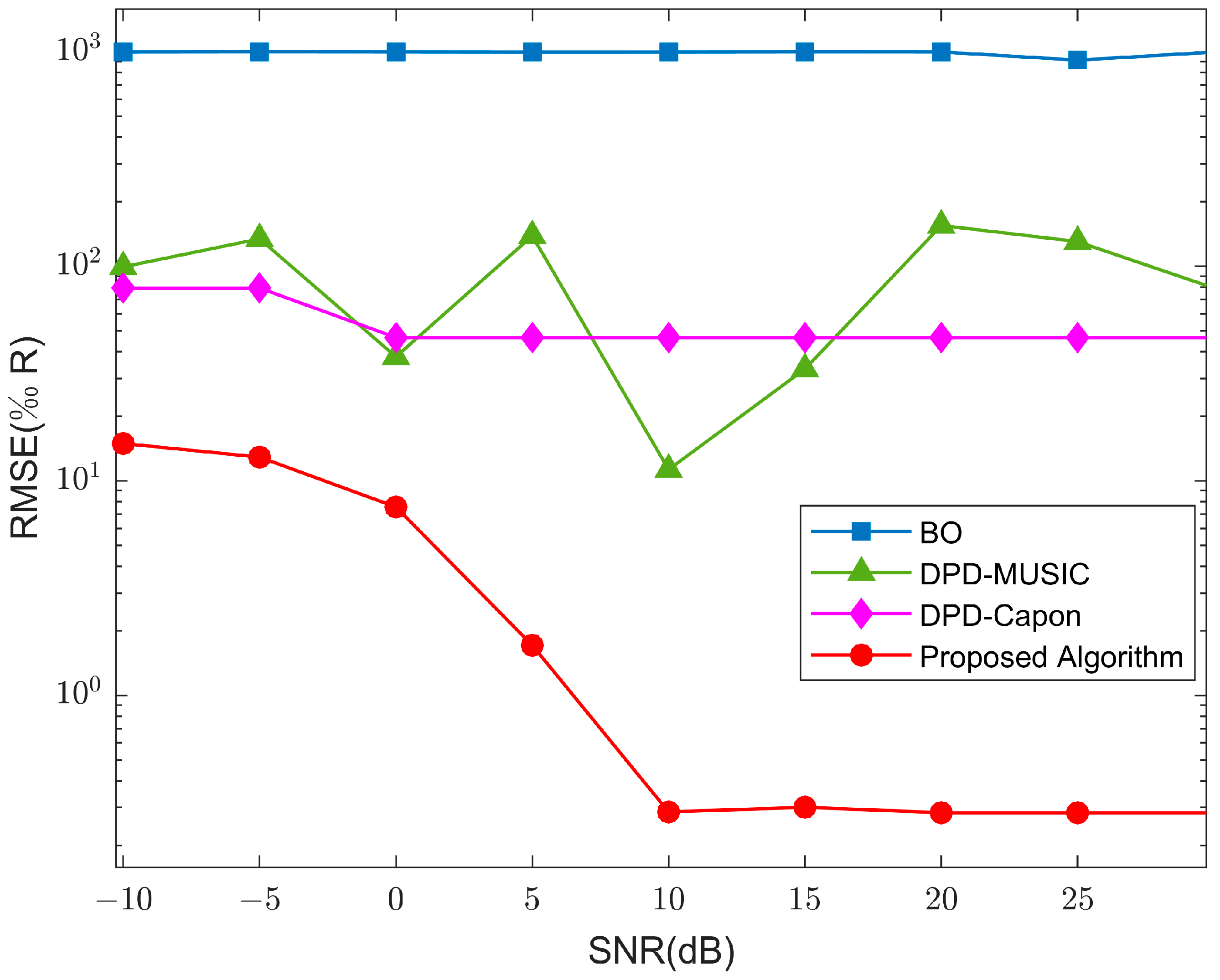
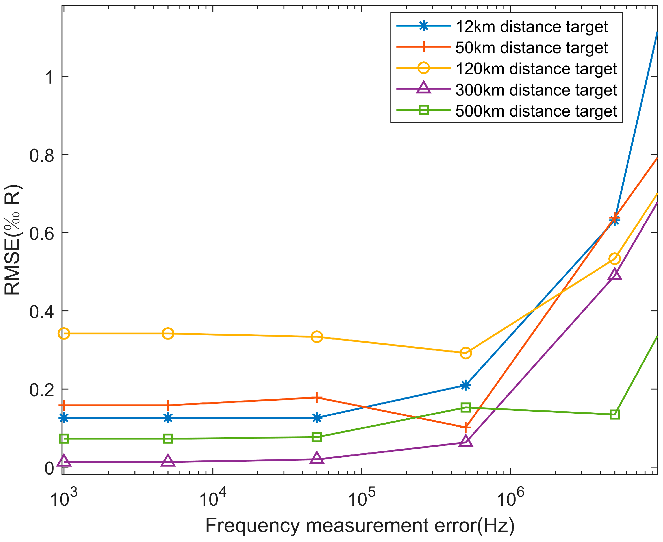
3.1. Simulation Results
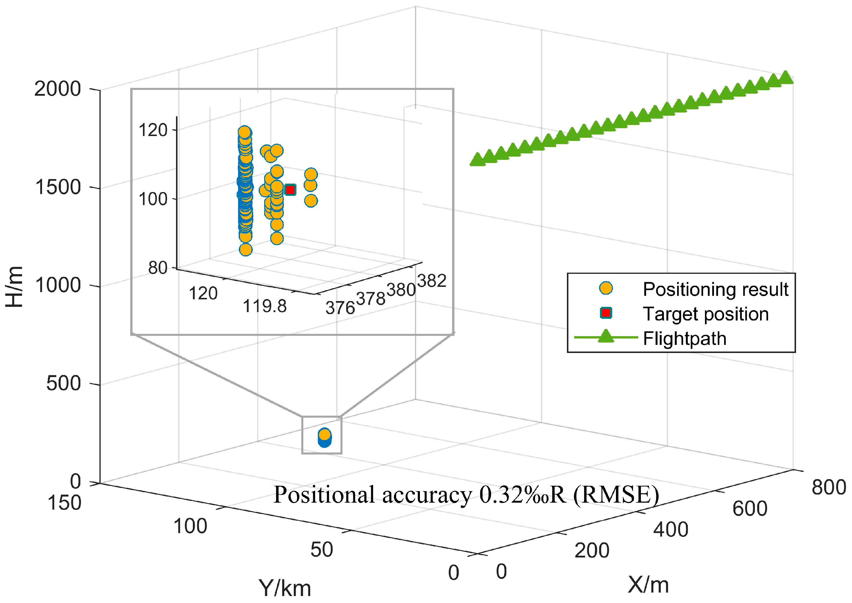
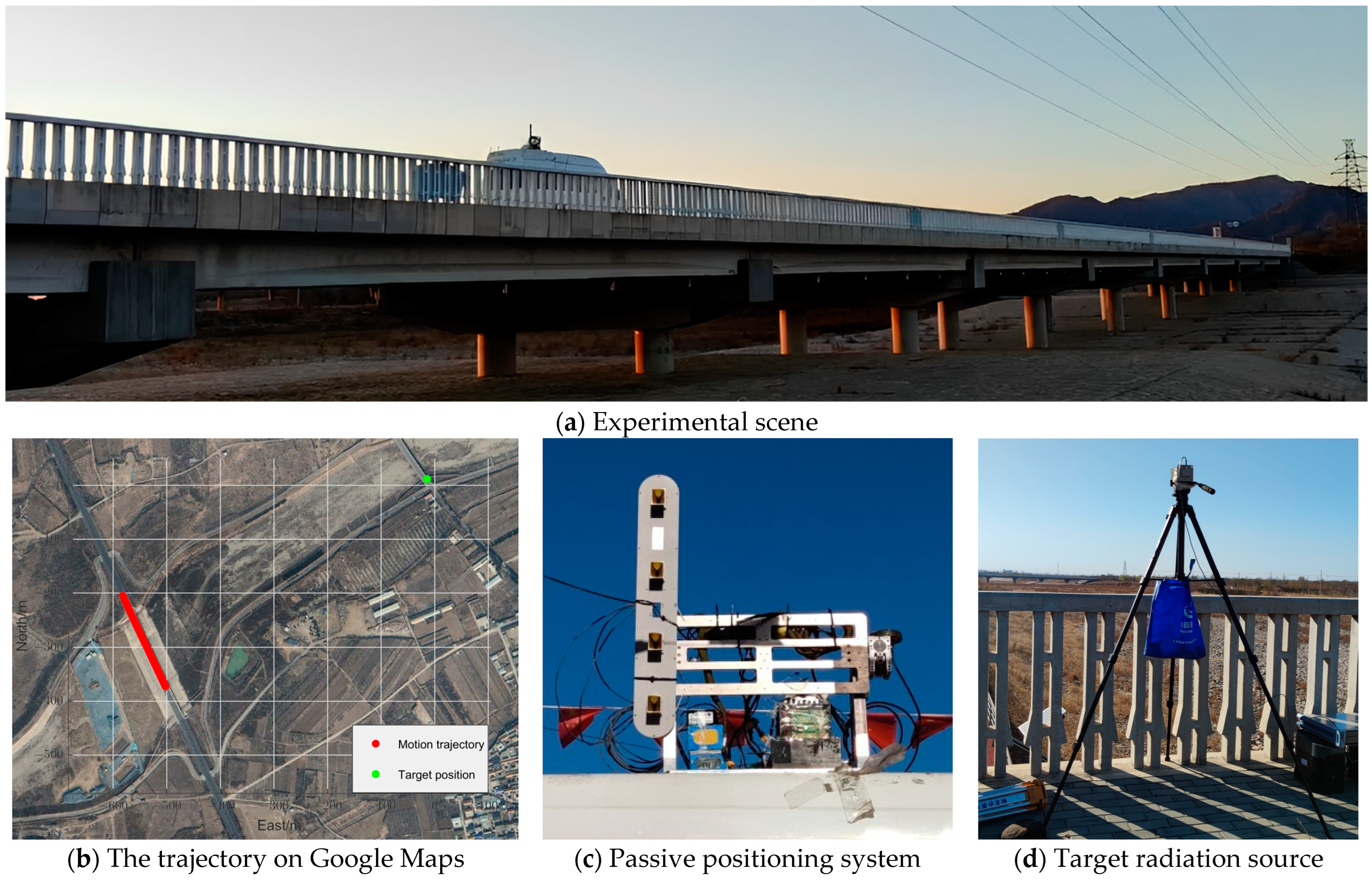
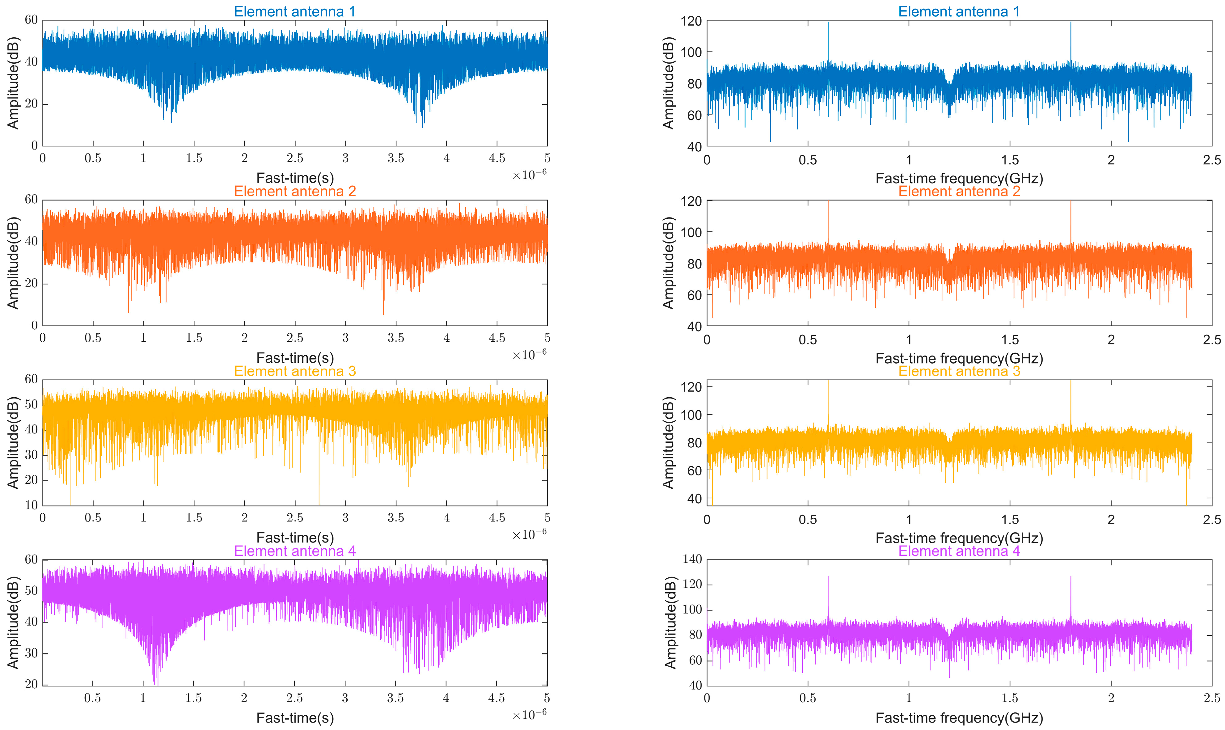
3.2. Experiment Results
4. Discussion
5. Conclusions
Author Contributions
Funding
Data Availability Statement
Acknowledgments
Conflicts of Interest
References
- Li, C.; Tanghe, E.; Fontaine, J.; Martens, L.; Romme, J.; Singh, G.; De Poorter, E.; Joseph, W. Multistatic UWB Radar-Based Passive Human Tracking Using COTS Devices. IEEE Antennas Wirel. Propag. Lett. 2022, 21, 695–699. [Google Scholar] [CrossRef]
- Li, A.; Huan, H.; Tao, R.; Zhang, L. Passive Synthetic Aperture High-Precision Radiation Source Location by Single Satellite. IEEE Geosci. Remote Sens. Lett. 2022, 19, 4010105. [Google Scholar] [CrossRef]
- Mao, Z.; Su, H.; He, B.; Jing, X. Moving Source Localization in Passive Sensor Network With Location Uncertainty. IEEE Signal Process. Lett. 2021, 28, 823–827. [Google Scholar] [CrossRef]
- Zhou, B.; Kim, N.; Kim, Y. A Passive Indoor Tracking Scheme with Geometrical Formulation. IEEE Antennas Wirel. Propag. Lett. 2016, 15, 1815–1818. [Google Scholar] [CrossRef]
- Yang, H.; Chun, J.; Chae, D. Hyperbolic Localization in MIMO Radar Systems. IEEE Antennas Wirel. Propag. Lett. 2015, 14, 618–621. [Google Scholar] [CrossRef]
- Liu, Y.; Xia, X.G.; Liu, H.W.; Nguyen, A.H.T.; Khong, A.W.H. Iterative Implementation Method for Robust Target Localization in a Mixed Interference Environment. IEEE Trans. Geosci. Remote Sens. 2022, 60, 5107813. [Google Scholar] [CrossRef]
- Wu, X.H.; Zhu, W.P.; Yan, J. A High-Resolution DOA Estimation Method With a Family of Nonconvex Penalties. IEEE Trans. Veh. Technol. 2018, 67, 4925–4938. [Google Scholar] [CrossRef]
- Li, P.; Li, J.F.; Ma, P.H.; Zhang, X.F. Array Orientation Adjustments Subject to Optimal Direct Position Determination Performance. IEEE Signal Process. Lett. 2022, 29, 115–119. [Google Scholar] [CrossRef]
- Tzafri, L.; Weiss, A.J. High-Resolution Direct Position Determination Using MVDR. IEEE Trans. Wirel. Commun. 2016, 15, 6449–6461. [Google Scholar] [CrossRef]
- Zhang, G.X.; Yi, W.; Varshney, P.K.; Kong, L.J. Direct Target Localization with Quantized Measurements in Noncoherent Distributed MIMO Radar Systems. IEEE Trans. Geosci. Remote Sens. 2023, 61, 5103618. [Google Scholar] [CrossRef]
- Le Gall, Y.; Socheleau, F.-X.; Bonnel, J. Matched-Field Processing Performance Under the Stochastic and Deterministic Signal Models. IEEE Trans. Signal Process. 2014, 62, 5825–5838. [Google Scholar] [CrossRef]
- Wang, Q.; Wang, Y.; Zhu, G. Matched Field Processing Based on Least Squares with a Small Aperture Hydrophone Array. Sensors 2017, 17, 71. [Google Scholar] [CrossRef]
- Wu, G.Z.; Zhang, M.; Guo, F.C. High-resolution direct position determination based on eigenspace using a single moving ULA. Signal Image Video Process. 2019, 13, 887–894. [Google Scholar] [CrossRef]
- Tirer, T.; Weiss, A.J. Performance Analysis of a High-Resolution Direct Position Determination Method. IEEE Trans. Signal Process. 2017, 65, 544–554. [Google Scholar] [CrossRef]
- Tirer, T.; Weiss, A.J. High Resolution Direct Position Determination of Radio Frequency Sources. IEEE Signal Process. Lett. 2016, 23, 192–196. [Google Scholar] [CrossRef]
- Song, K.; Feng, W. An Efficient Method of Direct Position Determination of Passive Radar with DIRECT Algorithm. J. Signal Process. 2020, 36, 149–154. [Google Scholar]
- Li, J.; Yang, L.; Guo, F.; Jiang, W. Coherent summation of multiple short-time signals for direct positioning of a wideband source based on delay and Doppler. Digit. Signal Process. 2016, 48, 58–70. [Google Scholar] [CrossRef]
- Kumar, G.; Ponnusamy, P.; Amiri, I.S. Direct Localization of Multiple Noncircular Sources with a Moving Nested Array. IEEE Access 2019, 7, 101106–101116. [Google Scholar] [CrossRef]
- Wang, Z.Q.; Sun, Y.M.; Wan, Q.; Xie, L.; Liu, N. A Modest Power Consumption Maximum Likelihood Direct Position Determination Approach for Multiple Targets With Moving Sensor Arrays. IEEE Sens. J. 2022, 22, 21885–21898. [Google Scholar] [CrossRef]
- Huang, Y.; Li, Y.; Liu, J. Long Distance Source Localization with Passive Synthetic Aperture Sonar. J. Electron. Inf. Technol. 2006, 28, 526–531. [Google Scholar]
- Li, T.; Li, Y.; Huang, H.; Chi, C. Robust estimation of target depth for towed array using synthetic aperture algorithm. J. Appl. Acoust. 2020, 39, 810–820. [Google Scholar]
- Zhao, S.; Sun, C.; Chen, X.; Yu, H. An Improved Passive Synthetic Aperture Sonar Alogorithm Application for Detecting of the Ship Radiated Noise. J. Electron. Inf. Technol. 2013, 35, 426–431. [Google Scholar] [CrossRef]
- Wang, Y.; Sun, G.; Yang, J.; Xing, M.; Yang, X.; Bao, Z. Passive Localization Algorithm for Radiation Source Based on Long Synthetic Aperture. J. Radars 2020, 9, 185–194. [Google Scholar]
- Wang, Y.; Sun, G.C.; Wang, Y.; Zhang, Z.; Xing, M.; Yang, X. A High-Resolution and High-Precision Passive Positioning System Based on Synthetic Aperture Technique. IEEE Trans. Geosci. Remote Sens. 2022, 60, 1–13. [Google Scholar] [CrossRef]
- Wang, Y.Q.; Sun, G.C.; Xing, M.D.; Zhang, Z.J. Performance Analysis and Parameter Design of Synthetic Aperture Passive Positioning. J. Electron. Inf. Technol. 2022, 44, 3155–3162. [Google Scholar]
- Yang, H.; Yang, J.; Liu, Z. Localizing Ground-Based Pulse Emitters via Synthetic Aperture Radar: Model and Method. IEEE Trans. Geosci. Remote Sens. 2023, 61, 5216714. [Google Scholar] [CrossRef]
- Wang, Y.; Dong, W.; Sun, G.C.; Zhang, Z.; Xing, M.; Yang, X. A CLEAN-Based Synthetic Aperture Passive Localization Algorithm for Multiple Signal Sources. IEEE J. Miniaturization Air Space Syst. 2022, 3, 294–301. [Google Scholar] [CrossRef]
- Wang, Y.; Han, L.; Zhang, X.; Sun, G.-C.; Zhang, Z.; Xing, M.; Yang, X. A Passive Signal Focusing Algorithm Based on Synthetic Aperture Technique for Multiple Radiation Source Localization. IEEE Trans. Geosci. Remote Sens. 2024, 62, 5206516. [Google Scholar] [CrossRef]
- Dong, W.L.; Wang, Y.Q.; Sun, G.C.; Zhang, Z.J.; Xing, M.D.; Yang, X.N. Synthetic Aperture Passive Localization for Frequency Hopping Signal. In Proceedings of the IGARSS 2022—2022 IEEE International Geoscience and Remote Sensing Symposium, Kuala Lumpur, Malaysia, 17–22 July 2022; pp. 1308–1311. [Google Scholar]
- Zhang, Y.; Bu, X.; Ge, X.; Xin, J.; Liang, X. An Iterative Motion Compensation Algorithm for Synthetic Aperture Passive Positioning. IEEE Signal Process. Lett. 2024, 31, 2680–2684. [Google Scholar] [CrossRef]
- Huang, C.Y.; Polydoros, A. Likelihood Methods for MPSK Modulation Classification. IEEE Trans. Commun. 1995, 43, 1493–1504. [Google Scholar]
- Swami, A.; Sadler, B.M. Hierarchical digital modulation classification using cumulants. IEEE Trans. Commun. 2000, 48, 416–429. [Google Scholar] [CrossRef]
- Wei, W.; Mendel, J.M. Maximum-likelihood classification for digital amplitude-phase modulations. IEEE Trans. Commun. 2000, 48, 189–193. [Google Scholar] [CrossRef]
- Wang, Y.; Liu, M.; Yang, J.; Gui, G. Data-Driven Deep Learning for Automatic Modulation Recognition in Cognitive Radios. IEEE Trans. Veh. Technol. 2019, 68, 4074–4077. [Google Scholar] [CrossRef]
- Shen, J.; Yi, J.; Wan, X.; Cheng, F.; Zhang, W. DOA Estimation Considering Effect of Adaptive Clutter Rejection in Passive Radar. IEEE Trans. Geosci. Remote Sens. 2022, 60, 5108913. [Google Scholar] [CrossRef]
- Zhang, X.; Tao, H.; Fang, Z.; Xie, J. Efficient DOA Estimation for Wideband Sources in Multipath Environment. Remote Sens. 2022, 14, 3951. [Google Scholar] [CrossRef]
- Lei, Y.; Tan, J.; Guo, W.; Cui, J.; Liu, J. Time-Domain Evaluation Method for Clock Frequency Stability Based on Precise Point Positioning. IEEE Access 2019, 7, 132413–132422. [Google Scholar] [CrossRef]
- Zhao, Y.; Li, Z.; Zhou, W.; Wu, H.; Bai, L.; Miao, M. Research on aging and frequency stability of crystal oscillator. J. Time Freq. 2018, 41, 267–275. [Google Scholar]
- Riley, W.J. Handbook of Frequency Stability Analysis; NIST Special Publication; US Department of Commerce, National Institute of Standards and Technology: Boulder, CO, USA, 2007.
- Xin, J.; Ge, X.; Zhang, Y.; Liang, X.; Li, H.; Wu, L.; Wei, J.; Bu, X. High-Precision Time Difference of Arrival Estimation Method Based on Phase Measurement. Remote Sens. 2024, 16, 1197. [Google Scholar] [CrossRef]
- Huang, C.; Chan, E.H.W.; Hao, P.; Wang, X. Wideband High-Speed and High-Accuracy Instantaneous Frequency Measurement System. IEEE Photon. J. 2023, 15, 7100408. [Google Scholar] [CrossRef]
- Wang, D.; Zhang, X.; Zhou, W.; Du, C.; Zhang, B.; Dong, W. Microwave Frequency Measurement Using Brillouin Phase-Gain Ratio With Improved Measurement Accuracy. IEEE Microw. Wirel. Compon. Lett. 2021, 31, 1335–1338. [Google Scholar] [CrossRef]


| Parameter | Value |
|---|---|
| Carrier frequency | 10.5 GHz |
| Moving speed | 60 m/s |
| Platform height | 2 km |
| Sampling frequency | 2.4 GHz |
| Synthetic aperture length | 800 m |
| Observation intersection angle | 0.38° |
| Antenna baseline | [0.17 m, 0.37 m, 0.58 m] |
| Target position | (380 m, 120 km, 100 m) |
| Algorithm | Run Time/s |
|---|---|
| DOA-LS | 0.0048 |
| MUSIC | 0.0345 |
| Proposed SRSVB Algorithm | 0.0050 |
| Algorithm | Run Time/s |
|---|---|
| BO | 1.50 |
| DPD-MUSIC | 115.62 |
| DPD-Capon | 109.76 |
| Proposed Algorithm | 2.99 |
| Parameter | Value |
|---|---|
| Carrier frequency | 11.5 GHz |
| Intermediate frequency | 1.8 GHz |
| Platform height (elevation) | 56.23 m |
| Moving speed | 10 m/s |
| Synthetic aperture length | 56.55 m |
| PRT | 1 ms |
| Sampling window length | 5 µs |
| Sampling frequency | 2.4 GHz |
| Antennae baseline | [0.17 m, 0,37 m, 0.58 m] |
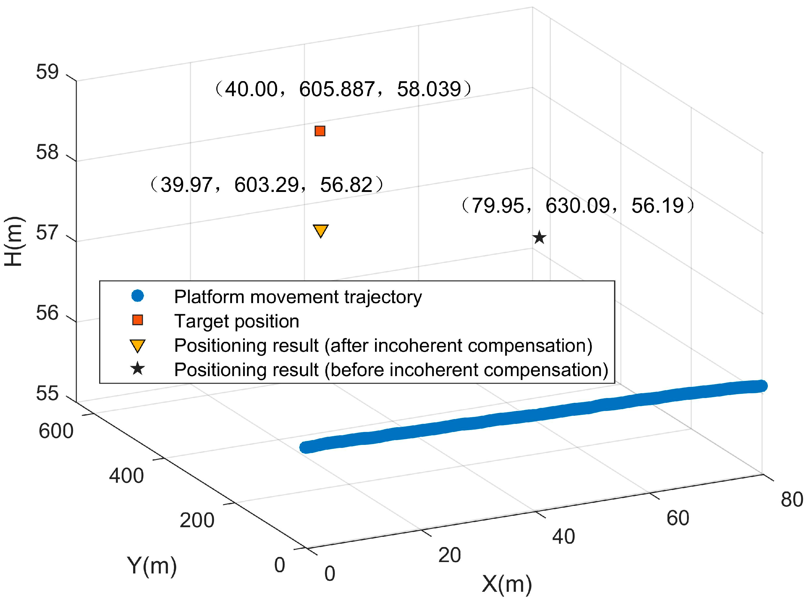
| Target position | [40.00 m, 605.887 m, 58.039 m] |
| Algorithm | Positioning Result | Positioning Error | Positioning Accuracy |
|---|---|---|---|
| BO | [40.01 m, 2.75 m, 57.57 m] | 603.14 m | 995.46 ‰R |
| DPD-MUSIC | [55.80 m, 550.75 m, 74.00 m] | 59.53 m | 98.25 ‰R |
| DPD-Capon | [5.00 m, 619.00 m, 81.20 m] | 43.97 m | 72.57 ‰R |
| Proposed Algorithm | [39.97 m, 603.29 m, 56.82 m] | 2.87 m | 4.73 ‰R |
Disclaimer/Publisher’s Note: The statements, opinions and data contained in all publications are solely those of the individual author(s) and contributor(s) and not of MDPI and/or the editor(s). MDPI and/or the editor(s) disclaim responsibility for any injury to people or property resulting from any ideas, methods, instructions or products referred to in the content. |
© 2025 by the authors. Licensee MDPI, Basel, Switzerland. This article is an open access article distributed under the terms and conditions of the Creative Commons Attribution (CC BY) license (https://creativecommons.org/licenses/by/4.0/).
Share and Cite
Zhang, Y.; Bu, X.; Guan, S.; Xin, J.; Jiang, Z.; Ge, X.; Li, M.; Li, Y.; Liang, X. A Cross-Track Interferometric Synthetic Aperture 3D Passive Positioning Algorithm. Remote Sens. 2025, 17, 932. https://doi.org/10.3390/rs17050932
Zhang Y, Bu X, Guan S, Xin J, Jiang Z, Ge X, Li M, Li Y, Liang X. A Cross-Track Interferometric Synthetic Aperture 3D Passive Positioning Algorithm. Remote Sensing. 2025; 17(5):932. https://doi.org/10.3390/rs17050932
Chicago/Turabian StyleZhang, Yuan, Xiangxi Bu, Sheng Guan, Jihao Xin, Zhiyu Jiang, Xuyang Ge, Miaomiao Li, Yanlei Li, and Xingdong Liang. 2025. "A Cross-Track Interferometric Synthetic Aperture 3D Passive Positioning Algorithm" Remote Sensing 17, no. 5: 932. https://doi.org/10.3390/rs17050932
APA StyleZhang, Y., Bu, X., Guan, S., Xin, J., Jiang, Z., Ge, X., Li, M., Li, Y., & Liang, X. (2025). A Cross-Track Interferometric Synthetic Aperture 3D Passive Positioning Algorithm. Remote Sensing, 17(5), 932. https://doi.org/10.3390/rs17050932