Quantifying the Accuracy of UAS-Lidar Individual Tree Detection Methods Across Height and Diameter at Breast Height Sizes in Complex Temperate Forests

Abstract

Unpiloted aerial systems (UAS) and light detection and ranging (lidar) sensors provide users with an increasingly accessible mechanism for precision forestry. As these technologies are further adopted, questions arise as to how select processing methods are influencing subsequent high-resolution modelling and analysis. This study addresses how specific individual tree detection (ITD) methods impact the successful detection of trees of varying sizes within complex forests. First, while many studies have compared ITD methods over several sites, algorithms, or sets of parameters based on a singular validation metric, this study quantifies how 10 processing methods perform across varying tree-height size quartiles and varying tree diameter at breast height (dbh) size quartiles. In total, over 1000 reference trees from 20 species within three complex temperate forest sites were analyzed at an average point density of 826.8 ${\mathrm{p}\mathrm{t}\mathrm{s}/\mathrm{m}}^2$. The results indicate that across four tree height size classes, the highest overall F-score (0.7344) was achieved with F-scores ranging from 0.857 for the largest and 0.633 for the smallest height size class. To further expand on this analysis, generalized linear models were used to compare the top performing and worst performing ITD method for each tree size variable and study site along a continuous gradient. This analysis suggests clear distinctions in the performance (true positive and false positive rates) based on tree sizes and ITD method. UAS-lidar users must ensure that demonstrated ITD processing methods are validated in ways that communicate their relative effectiveness for trees of all sizes. Without such consideration, the results of this study show that forest surveys and management conducted using these technologies may not accurately characterize trees present within complex forests.

1. Introduction

The measurement of forest characteristics is an important step towards understanding forest ecosystems [1,2,3]. For many decades, remote-sensing technologies have been leveraged to provide valuable supplemental data to make the collection of forest measurements more efficient and exhaustive [4,5,6,7]. The use of aerial photography and digital imagery for photo interpretation and photogrammetry in forest monitoring and management is a well-established, yet still developing, discipline. Active remote-sensing technologies, such as light detection and ranging (lidar) and radar systems have further transformed the way we measure and observe forests in the 21st century [8,9,10,11]. Research into the use of lidar in forestry has demonstrated that these sensors are effective in measuring forest structure [12]. To date, lidar applications have been demonstrated from satellite [7,13,14], airborne [15,16], terrestrial [17,18,19], mobile [20,21], and unpiloted aircraft systems [22,23]. The advantages and disadvantages of various lidar systems are discussed in [24]. Growing interest in the commercial, research, and management fields has led to the development of lidar sensors capable of sufficiently high point densities to measure individual trees. These novel lidar sensors are also attainable at a fraction of the cost of sensors available even five years ago [25,26]. The pairing of such sensors with unpiloted aerial systems (UAS or UAV) offers an approach to surveying forests at practical or even commercial scales and accuracies [4,22,27,28,29,30]. An often-critical step in this approach, however, is the detection of individual trees, which still incurs three notable difficulties. These are: (1) poor detection rates within complex forests, (2) uncertainty in the performance of various individual tree detection (ITD) methods, and (3) insufficient evaluation of the performance of such methods across tree size classes.

UAS-lidar, when applied to planted forests, have demonstrated an exceptional performance for surveying individual trees [27,31,32]. Many conventional methods for individual tree detection, however, have had difficulty with mixed-species, multi-layered, forests due to the occlusion of small trees or complex crowns of deciduous trees [33,34,35]. In Yin et al. [36], for example, the detection rate for individual mangrove trees was problematic due to the clumping of tree stems. Similarly, You et al. [37] showed that the accuracy of segmentation of individual mangrove trees was influenced by stand complexity. Liang et al. [38] demonstrated that the performance of measuring forest parameters decreases with increasing stand complexity. Natural forests, such as those in the eastern United States often contain dense, multi-layered canopies [39,40]. UAS-lidar data must be accurate and complete enough to effectively characterize forest stands, even among natural forests [41].

A compounding challenge for UAS-lidar analyses of complex natural forests has been the limited validation of processing methods across trees of different sizes. Several studies have found the performance of ITD methods to be dependent on the processing method choices. Such ITD processing method choices include the size of the moving window function or algorithm choice [35,42,43]. These largely open-ended options lead to uncertainty for new UAS practitioners as they navigate the most effective methods for using UAS-lidar data for precision forestry. As UAS-lidar technologies continue to be developed and become more affordable, it is likely that many will turn to ITD algorithms originally designed and tested on UAS structure from motion (SfM) models. The transferability between photogrammetric point clouds and lidar point clouds remains unclear. Even when adopting UAS-lidar specific parameters, past studies have found that successive missions across neighboring properties could be improved using unique processing settings [44]. Additionally, if users adopt ITD algorithms or processing settings based on the findings of studies which are even five to ten years old, the differences in UAS-lidar data point densities could introduce an unintentional source of error. Wallace et al. [45] performed an early study on tree-detection algorithms when varying segmentation methods and UAS-lidar point cloud densities. In their study, higher density point clouds demonstrated lower tree detection (omission) error; however, the point cloud densities ranged between 5 ${\mathrm{p}\mathrm{t}\mathrm{s}/\mathrm{m}}^2$ and 50 ${\mathrm{p}\mathrm{t}\mathrm{s}/\mathrm{m}}^2$ which is over an order of magnitude lower than what is readily achievable today. For example, UAS-lidar research published in the last two years has been conducted with point densities ranging from 100 ${\mathrm{p}\mathrm{t}\mathrm{s}/\mathrm{m}}^2$ to 1000 ${\mathrm{p}\mathrm{t}\mathrm{s}/\mathrm{m}}^2$ [46,47,48]. Such a difference in sensor capability makes comparison to earlier established methods less applicable [44,46]. Lastly, while many studies have tested and reported ITD accuracies, few have considered the performance of such methods more comprehensively than a singular overall detection rate [49,50,51,52]. Over-detection of large trees (i.e., false positive detections or commission error) and under-detection of small trees (false negative detections or omission error) has been a challenge for UAS digital photogrammetry [35]. Understory trees may be important for several reasons including wildlife resources, management planning, carbon accounting, and accurate forest type mapping. These trees are also a key to microclimate observations, competition, and future forest dynamics [53]. By not quantifying tree-detection accuracy across tree size classes, current methods for the UAS-lidar analysis of individual trees could be misleading practitioners as they study complex forests. For example, by introducing error into estimating the number of stems per unit area or skewing tree level measurements towards larger trees and those in the upper canopy [45,54].

This study addresses three crucial aspects of a knowledge gap for future practitioners of UAS-lidar in forestry who are seeking a framework for performing analyses at the individual tree scale [24,55]. First, through investigating the relative effectiveness of various technologically accessible ITD methods. Here, technologically accessible methods include algorithms and processing settings which can be performed with minimal coding or software experience. Second, by documenting the performance of such ITD methods across a range of tree height and diameter at breast height (dbh) sizes, which are commonly found in complex forests. Third, by demonstrating the results of such methods using UAS-lidar point densities which are more comparable to sensors which are increasingly available to today’s researchers and land managers.

2. Materials and Methods

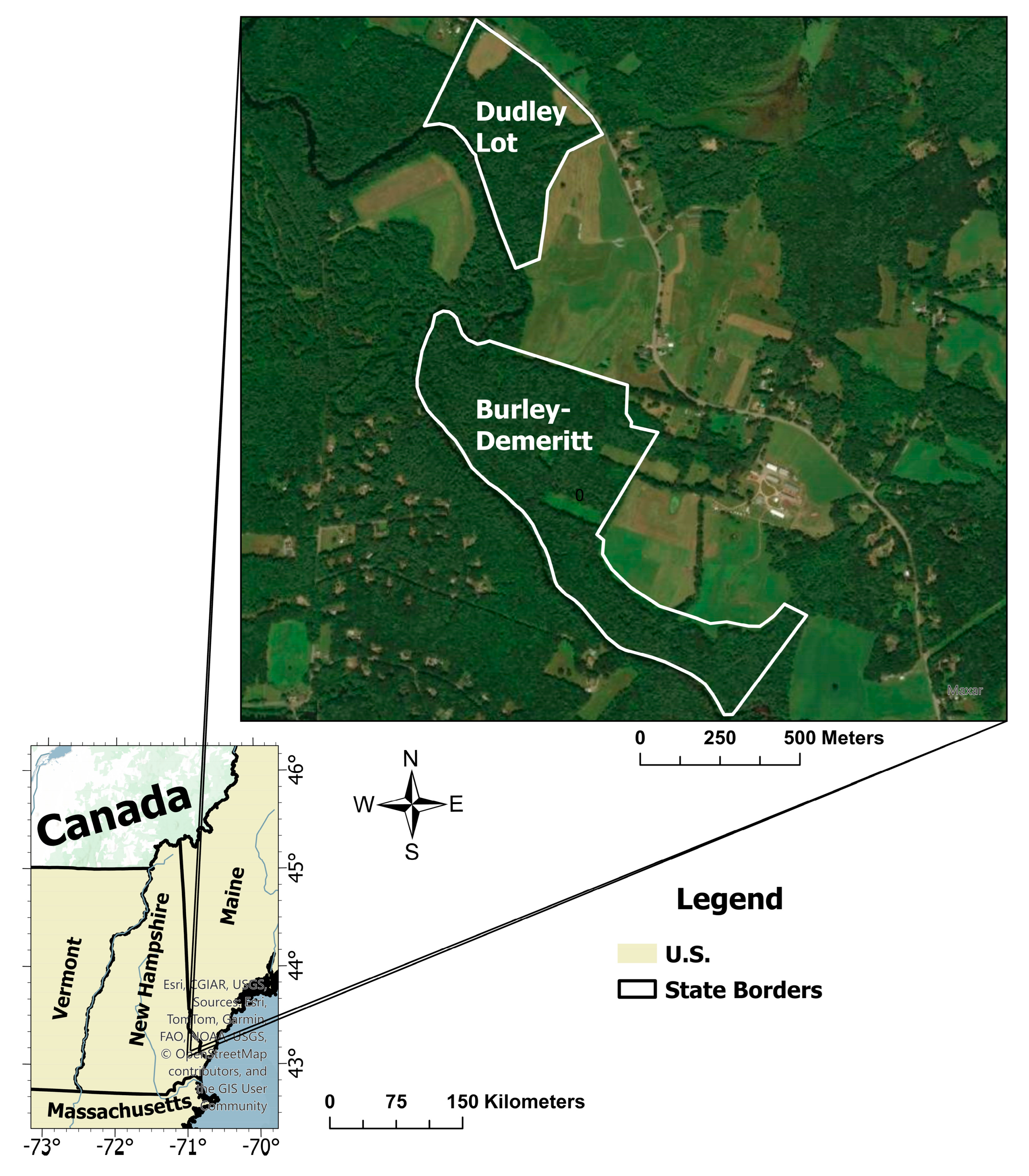
2.1. Study Sites

Three woodlands located within the eastern deciduous forest biome were surveyed during this research. The first two woodlands were located in Lee, New Hampshire (NH, USA) and are managed as research and educational forests by the University of New Hampshire (UNH) [56] (Figure 1). Dudley Lot (hereafter referred to as Dudley) is a 42.5-hectare (ha) property of which 16.19 ha are forested. Six total forest stands (management units) make up the Dudley woodlands [44]. One stand was harvested in the mid-1980s and is now an early successional forest. The remainder parallels the regional mixed-forest composition. Burley-Demeritt is an 82.15 ha parcel located less than 1 km away. On this parcel, 52.6 ha are forested, while the rest is home to the UNH organic dairy farm [56]. Timber inventories for these properties conducted in 2015 reported a total of over 20 indigenous tree species [56].

The third woodland is a subcomponent of the UNH Woodman Horticulture farm. This parcel, located in Durham, NH, is also managed by UNH primarily for research use. Out of the total 109 ha, 81.7 ha of this parcel are forested. Similarly to both other study sites, during the most recent forest inventory, over 20 indigenous tree species were recorded [57]. This site was selected due to the recent establishment of a marteloscope plot within a southwestern compartment of this property (Figure 2), which is described further in the next section.

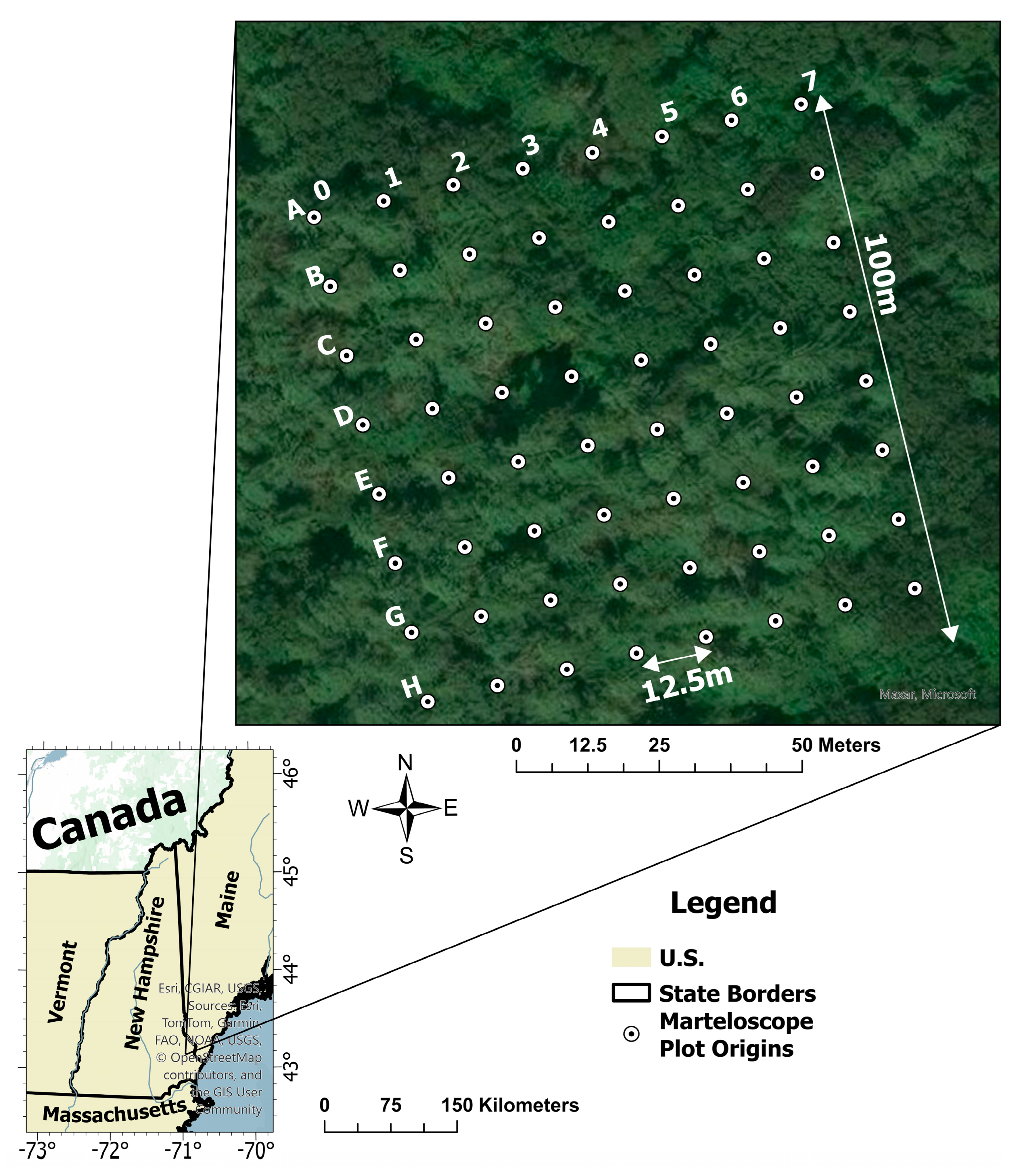
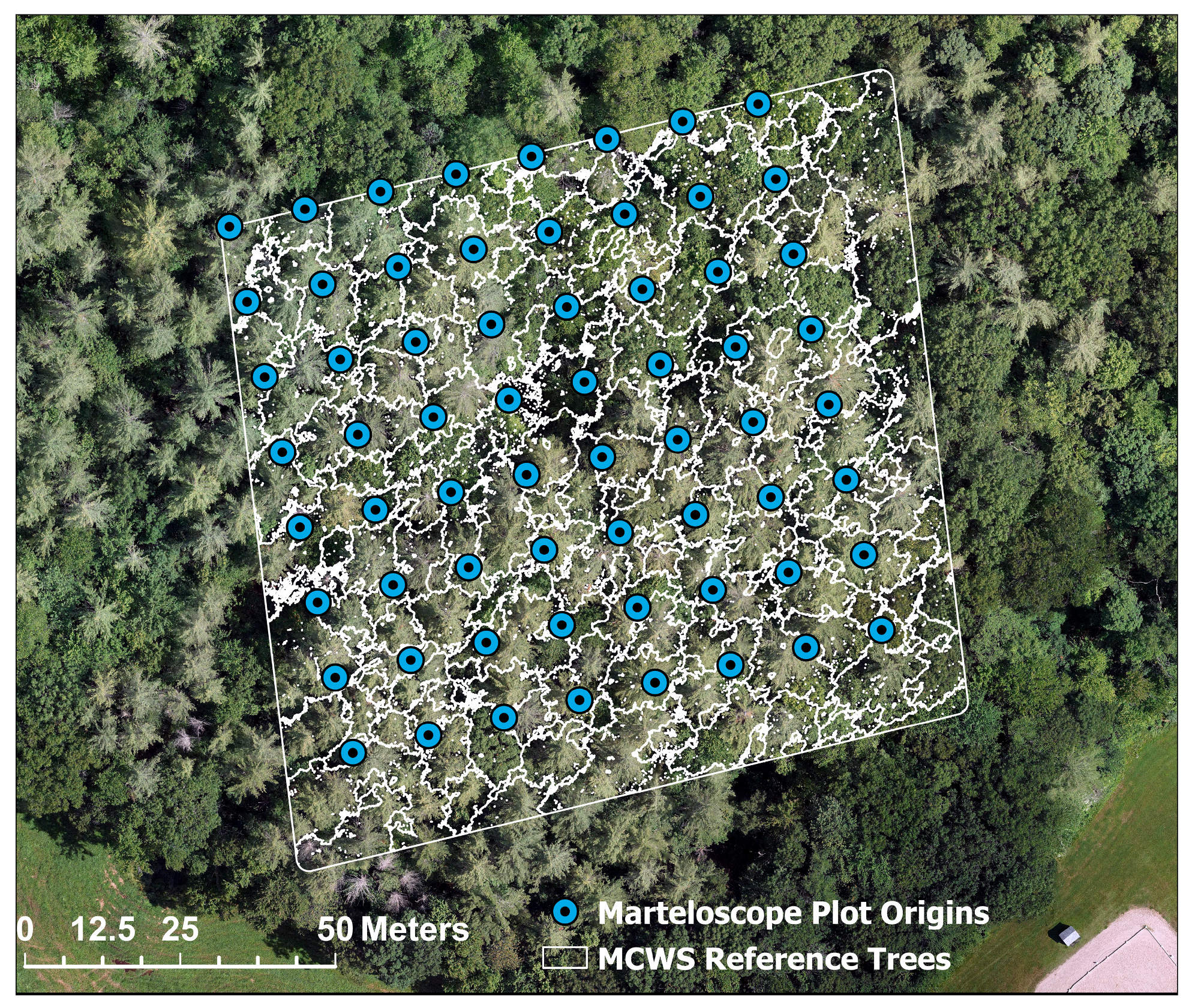
2.2. Reference Data

Reference trees were measured for the Dudley and Burley-Demeritt study sites in July and August of 2022 by repeating the 2015 UNH continuous forest inventory (CFI) plot sampling design [56]. The original plot design established for both properties placed one variable radius plot every hectare, maintaining a grid spacing. At each plot, trees greater than 10.16 cm (4 inches) in dbh were surveyed using a basal area factor (BAF) 4.59 ${\mathrm{m}}^2/\mathrm{h}\mathrm{a}$ prism (BAF 20 in imperial units). High-precision coordinate information was recorded for each measured tree using an EOS Arrow 100 GPS (Quebec, QC, Canada) [58]. The average estimated positional error for these tree locations was 1.44 m (std. dev. ± 0.71 m). Next, the species and dbh for these trees were recorded. In total, 357 trees were surveyed. The dbh values for these trees ranged from 11.43 cm to 114.3 cm. A concurrent Big BAF survey was conducted on these same trees using a BAF of 17.2 ${\mathrm{m}}^2/\mathrm{h}\mathrm{a}$ prism (BAF 75 in imperial units) [1,59].

Two measurement practices were used to revisit these plots from 2015 and collect updated individual tree-height measurements. First, all height trees (those measured as part of the Big BAF plots) still standing from the 2015 forest inventory were measured during the 2022 site visits. Tree heights were measured using a Vertex hypsometer (Haglof Sweden, Langsle, Sweden) [44]. Second, to increase the tree-height sample size across both properties, additional trees originally surveyed during the 2015 forest inventory based on the smaller (BAF) 4.59 ${\mathrm{m}}^2/\mathrm{h}\mathrm{a}$ prism also had their heights measured. These trees were selected across both properties to more equally sample trees of varying height from among the initial CFI plot measurements. In total, 162 tree heights were measured. These tree heights ranged from 12.22 m to 39.04 m.

For both measurements, height and dbh, tree sizes were subdivided into four quantiles based on their maximum values (

Table 1. Tree height (m) and diameter at breast height (dbh) size quartile measurement ranges for the Lee study sites (Dudley and Burley-Demeritt). All numbers are rounded to 2 decimal places. Tree sizes are smallest to largest from left to right. Size 4 are the smallest trees for each parameter, size 1 are the largest trees for each parameter.

	4	3	2	1
Height (m)	12.22 to 23.74	23.84 to 28.16	28.19 to 32.25	32.31 to 39.04
DBH (cm)	11.43 to 28.45	28.96 to 40.64	40.89 to 52.83	52.83 to 114.3

). This division of tree sizes was used to ensure that the number of sample trees for each size class was comparable as possible. The size class quantiles for both tree height and dbh were ordered with class 4 being the smallest and class 1 being the largest. For the dbh measurements, this resulted in class-specific sample sizes of 89, 89, 89, and 90 (1, 2, 3, and 4). For the tree height measurements, this resulted in class-specific sample sizes of 40, 40, 41, and 41 for each quartile (1, 2, 3, and 4).

Each of the 357 trees located in the field were visually matched to trees identified in a high-resolution natural color UAS-orthoimage created from imagery collected during the UAS-lidar flights. The spatial resolution of these orthoimages for each study site was smaller than 3 cm (1.1 cm to 2.6 cm). The trees crowns were then manually digitized by a pair of trained remote-sensing technicians and given both a height and dbh size class label. These 357 and 162 tree crown polygons (dbh and height class samples, respectively) served as reference data for the ITD accuracy assessment based on the Lee property analysis.

At the third and final study site, the Woodman Horticulture farm, reference trees were measured as part of a 1 ha marteloscope plot, established based guidance in the I+ sampling design [60,61]. The marteloscope plot sampling design is an internationally recognized format for conducting research on and teaching from a standardized forest survey [62,63,64]. This marteloscope plot consisted of a 100 m by 100 m square, in which every tree, living or dead, greater than 7.5 cm dbh was inventoried. After an initial assessment of the potential plot location, the northwest corner of the plot was marked using a high precision Arrow 100 GPS [58]. Next, internal cells were meticulously laid out, within which each tree meeting the dbh threshold was surveyed. Once all of the trees within a cell were measured, subsequent cells were established column by column within the 1 ha boundary. In total, 666 trees were measured during this survey. After the entire plot was established, a secondary plot sampling phase is initiated. During this second plot sampling phase, a 10% systematic sample of trees was measured for total height and four crown radii using a Vertex hypsometer. This second sampling phase recorded 62 tree heights. Based on these two sampling phases, the dbh values ranged from 7 cm to 69.7 cm with an arithmetic mean of 22.79 cm (15.1 cm standard deviation). The height measurements ranged from 0.2 m to 37.7 m with an arithmetic mean of 18.79 m (9.04 m standard deviation).

The trees measured throughout the marteloscope plot were georeferenced based on their bearing (using a Suunto compass) and horizontal distance from each internal cell origin using a combination of the ‘Distance and Bearing to Line’ and ‘Line to End Points’ tools in ArcGIS Pro (v 3.1) (Redlands, CA, USA). Three of the trees were removed due to errors in the recorded measurements or positions. Another two samples were removed while generating the reference tree crown areas (due to poor geometry). The remaining 661 trees were each used as reference samples for the detection of individual trees based on their dbh and height size quantiles (

Table 2. Tree height (m) and diameter at breast height (dbh) size class measurement ranges for the marteloscope plot. All numbers are rounded to one decimal place. Trees sizes are smallest to largest from left to right. Size 4 are the smallest trees for each parameter, size 1 are the largest trees for each parameter.

	4	3	2	1
Height (m)	1.9 to 11.9	12.1 to 19.0	19.3 to 25.2	25.8 to 37.7
DBH (cm)	7.0 to 10.7	10.7 to 17.3	17.3 to 30.8	31.0 to 69.7

).

2.3. UAS-Lidar Data Collection

The UAS-lidar data were collected for each of the three study sites using the same DJI Matrice 300 RTK (M300 RTK) (Shenzen, China) and Zenmuse L1 lidar sensor. The DJI Zenmuse L1 has promising performance, matching or exceeding the manufacturer values in some instances during early studies [65]. Thorough descriptions of the DJI M300 RTK and Zenmuse L1 technical specifications and performance can be found in Stroner et al. [65]. The sensor specifications are listed as: 240,000 points per second, up to 3 returns per pulse, a 5 cm vertical accuracy, a 10 cm horizontal accuracy, a maximum detection range of 450 m, and an integrated 20 MP natural color camera for automatic point cloud colorization. Paired with this sensor and UAS was the DJI D-RTK 2 global navigation satellite system (GNSS) base station. This base station provided real-time corrections of the GPS data during all missions. Each of the missions (flights) were pre-programmed using the DJI Enterprise smart controller DJI pilot app (v7.0.1.). A .kml file for each of the three study areas was uploaded as the corresponding mission areas.

Both Lee properties, Dudley and Burley-Demeritt, were flown in July and August 2022. Dudley was completed in 2 flights, while Burley-Demeritt was completed in 3 flights given their size and geometry. All flights were conducted at 100 m above the ground, a 7.5 $\mathrm{m}/\mathrm{s}$ flight speed and with an 85% side overlap and 80% forward overlap (forward overlap is specific to the concurrently collected imagery) [44,66]. The L1 sensor was set to a 160 Hz scanning frequency, triple return mode, and enabled to collect natural color imagery. The resulting (estimated) scanning density for these flights was 799 ${\mathrm{p}\mathrm{t}\mathrm{s}/\mathrm{m}}^2$. At the beginning of each flight, end of each flight, and ends of each flight line, the mission planning software automatically conducted a GNSS and sensor calibration, to maintain the positional accuracy throughout the missions.

The Horticulture farm marteloscope plot was flown in August 2023, during the same month in which the field sampling was conducted. This study area was flown with similar flight planning settings as the Lee parcels. Given the size of the mission area, the full plot was completed in a single flight. The flying height was set to 100 m, the side overlap was 85%, the forward overlap (i.e., endlap) was 80%, the scanning frequency was 160 Hz, and the sensor recorded triple returns. Simultaneous natural color imagery was collected during this flight. The resulting (estimated) scanning density was 882.4 ${\mathrm{p}\mathrm{t}\mathrm{s}/\mathrm{m}}^2$ (Figure 3).

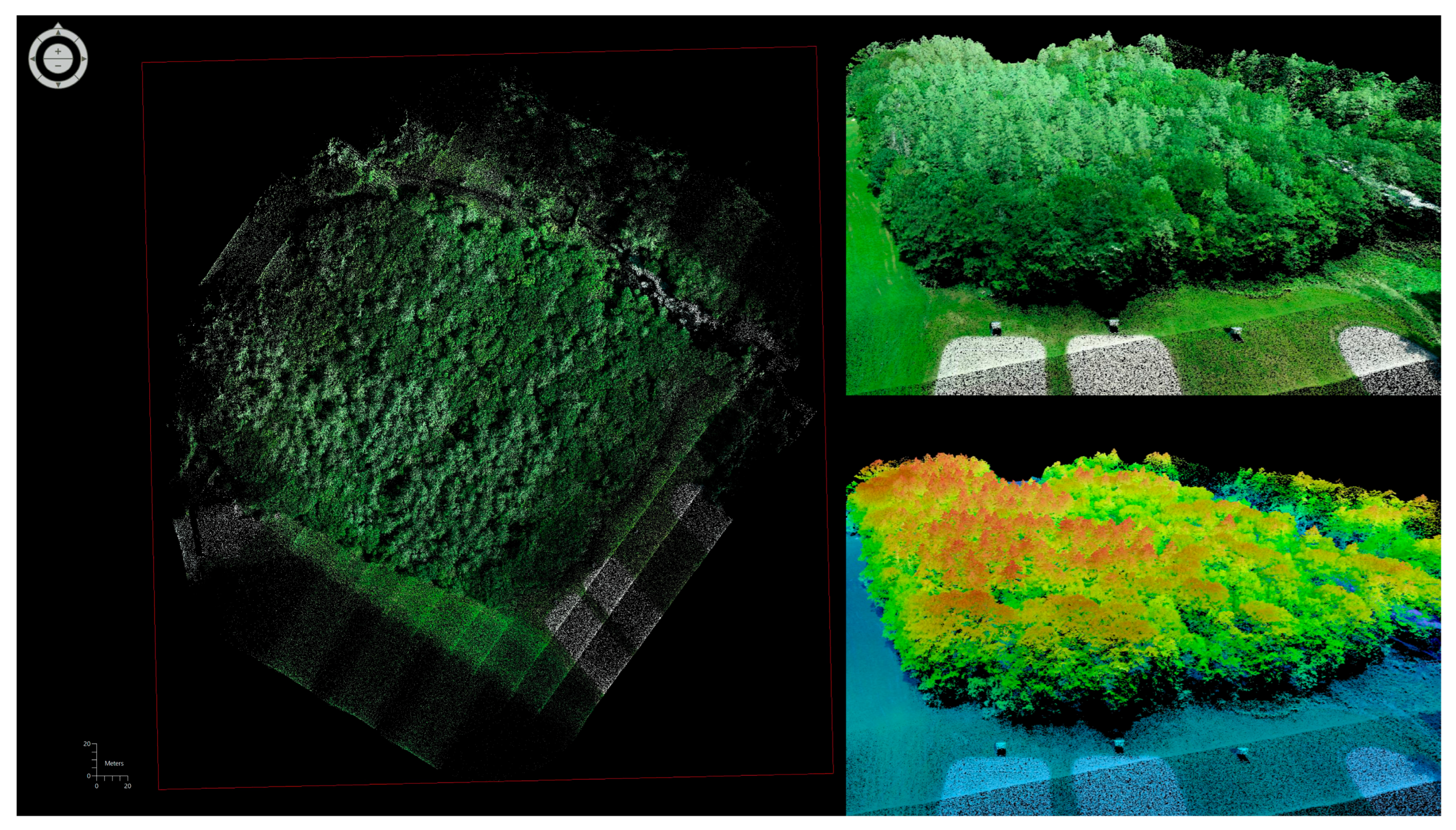
2.4. UAS-Lidar Data Pre-Processing

The lidar files and natural color imagery for each complete study site was individually imported into the DJI Terra software (v3.6.0; Shenzen, China). The DJI Terra software was used to pre-process the remotely sensed data, creating a singular, merged, colorized (.las) lidar point cloud and natural color orthomosaic for each site. The lidar point cloud was processed at its full (100%) resolution). Both the point cloud and orthomosaic were exported in the WGS 84/UTM 19N projected coordinate system.

The lidR package (R v4.3.3) was used to generate additional lidar products as well as for all individual tree detection (both fixed and variable window sizes) processing [67,68,69,70]. This open-source package provides a foundation for processing large, high-density point clouds, with a variety of leading statistical methods [69,70]. To generate statistically appropriate raster products, such as the digital surface model (DSM or terrain model) and canopy height model (CHM), the nominal point spacing for each study site was calculated using the provided point density conversion (Equation (1)) [15]. Before generating each of the intermediate raster products, the ground points were filtered and classified based on the Zhang et al. [71] cloth simulation function. Next, the digital terrain models (i.e., ground) were interpolated based on the lidR built-in kriging functions [67,72,73]. Third, the las point clouds were then normalized, to heights above the ground, based on the continuous functions [68]. Lastly, a CHM for each site was rasterized based on the point density (Equation (1)) creating raster surfaces of 3.6 cm, 3.6 cm, and 3.4 cm, for Dudley, Burley-Demeritt, and marteloscope plot, respectively [15]. Voids in the CHM were filled during this stage using a 5 cm point to radius function for all sites. These three CHMs were used for the ITD analysis.

Equation (1). Point density (PD) calculation based on the nominal point spacing (NPS or PS) [15].

$$PD={\displaystyle \frac{1}{{PS}^2}}$$

(1)

2.5. Tree Detection Methods

A total of seven fixed and three variable window size functions were applied to the three study site CHMs. All functions were performed using the R lidR package [67]. The full description of all 10 functions is given in

Table 3. Ten unique methods for performing the raster (canopy height model)-based individual tree detection process based on either fixed window (FW) or variable window functions (VWFs). Each method is based on a generic testing parameter or literature relevant to this region.

Window Function	Description	Method	Citation
Fixed	Generic FW size.	50 cells (~1.5 m)
Fixed	Generic FW size.	100 cells (~3 m)
Fixed	Minimizing under-segmentation, to support individual tree classification.	1.65 m	[54]
Fixed	Reference tree crown size average for recent study in this region.	4.5 m	[37]
Fixed	Reference tree crown size average for a deciduous plot for recent study in this region.	4.51 m	[45]
Fixed	Reference tree crown size average for a coniferous plot for recent study in this region.	4.58 m	[45]
Fixed	Average tree crown radius of digitized crowns from previous study at Lee sites	2.767727 m	[44]
Variable	Mixed forest equation from Popescu and Wynne [12]	$\mathrm{C}\mathrm{W}=2.51503+0.00901\ast {\mathrm{H}}^2$ ${\mathrm{R}}^2=0.59$	[12]
Variable	R: ForestTools default parameters	$\mathrm{C}\mathrm{R}=\mathrm{H}\ast 0.05+0.6$	[12,74]
Variable	Forest inventory data (2015) regression	$\mathrm{C}\mathrm{R}=4.7802+0.1104\ast \mathrm{H}$ ${\mathrm{R}}^2=0.14$	[37,56]

. The fixed window size functions (FW) were based on recent literature conducted on local forests using either UAS digital photogrammetry or UAS lidar [37,44,45,54]. These FW functions represent a combination of optimal results from previous studies, empirically formulated averages for crown diameters from previous studies, and generic cell size (e.g., 50 cell and 100 cell windows). The variable window size functions (VWFs) were based on (1) regression results from Popescu and Wynne [12] for mixed composition forests, (2) a linear regression based on the guide for the R ForestTools package (v1.0.2) [74], and (3) a linear regression between crown width and tree height based on the Lee study sites’ original field reference data [37,56]. The regression equations for these three VWFs are given below as Equation (2), Equation (3), and Equation (4), respectively.

Equation (2): Popescu and Wynne [12] mixed forest quadratic regression equation for crown width (CW) based on tree height (H).

$$\mathrm{C}\mathrm{W}=2.51503+0.00901\ast {\mathrm{H}}^2$$

(2)

Equation (3): Tree crown regression for crown radius (CR) based on tree height (H) based on the default parameters found within the R ForestTools guide [74].

$$\mathrm{C}\mathrm{R}=\mathrm{H}\ast 0.05+0.6$$

(3)

Equation (4): Field inventory measurement tree crown regression for crown radius (CR) based on tree height (H) from the Lee, NH study sites.

$$\mathrm{C}\mathrm{R}=4.7802+0.1104\ast \mathrm{H}$$

(4)

2.6. Individual Tree Detection Performance

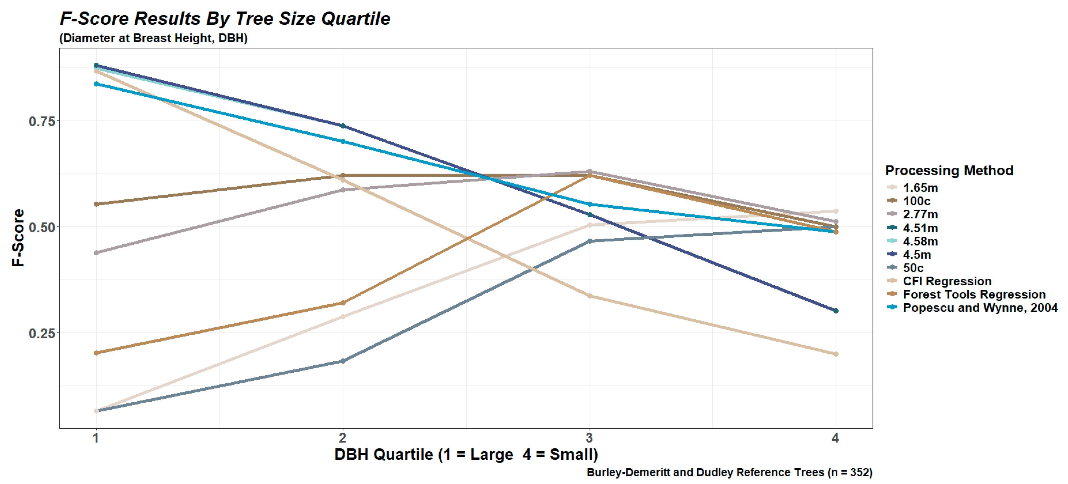
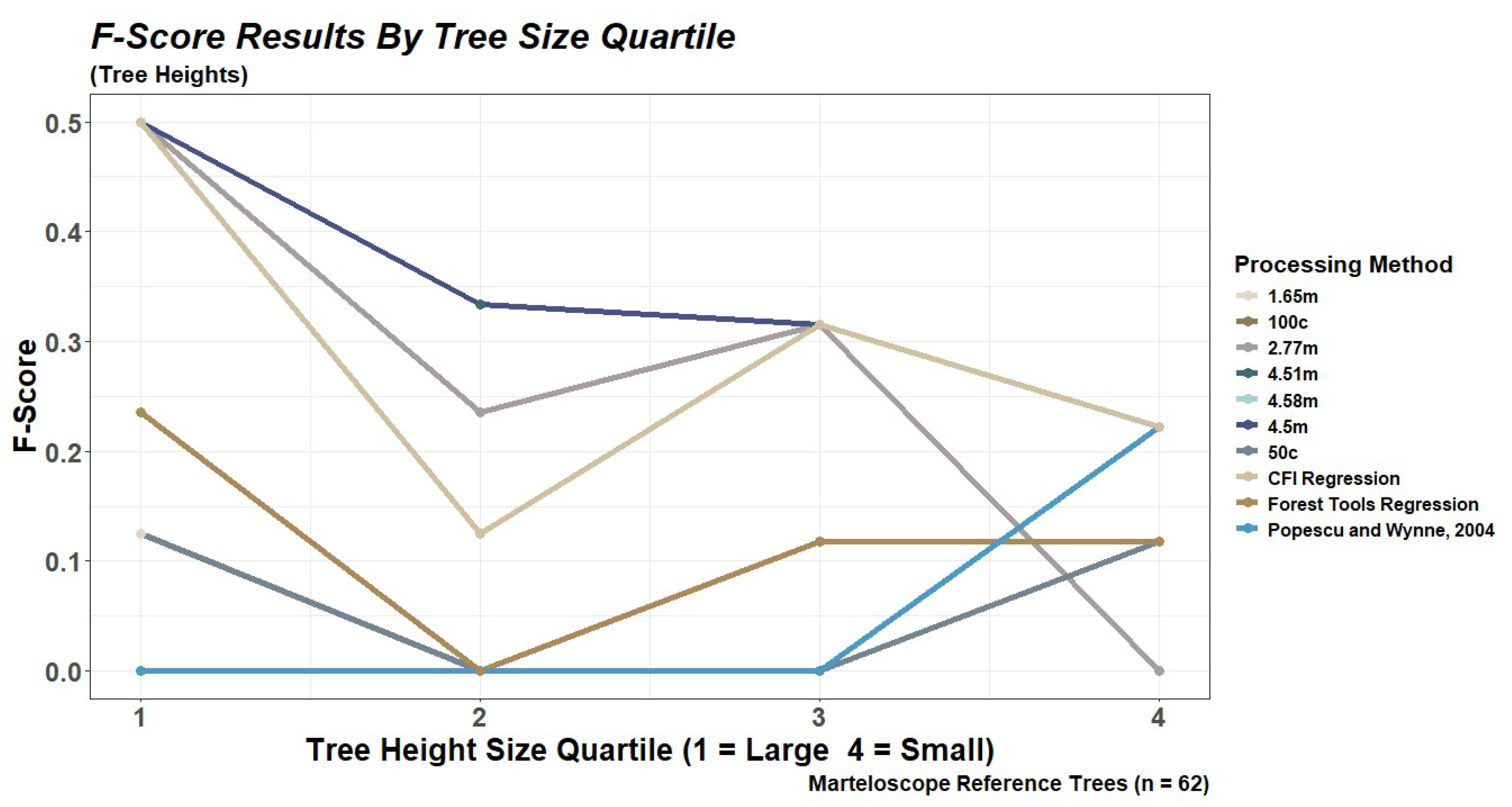
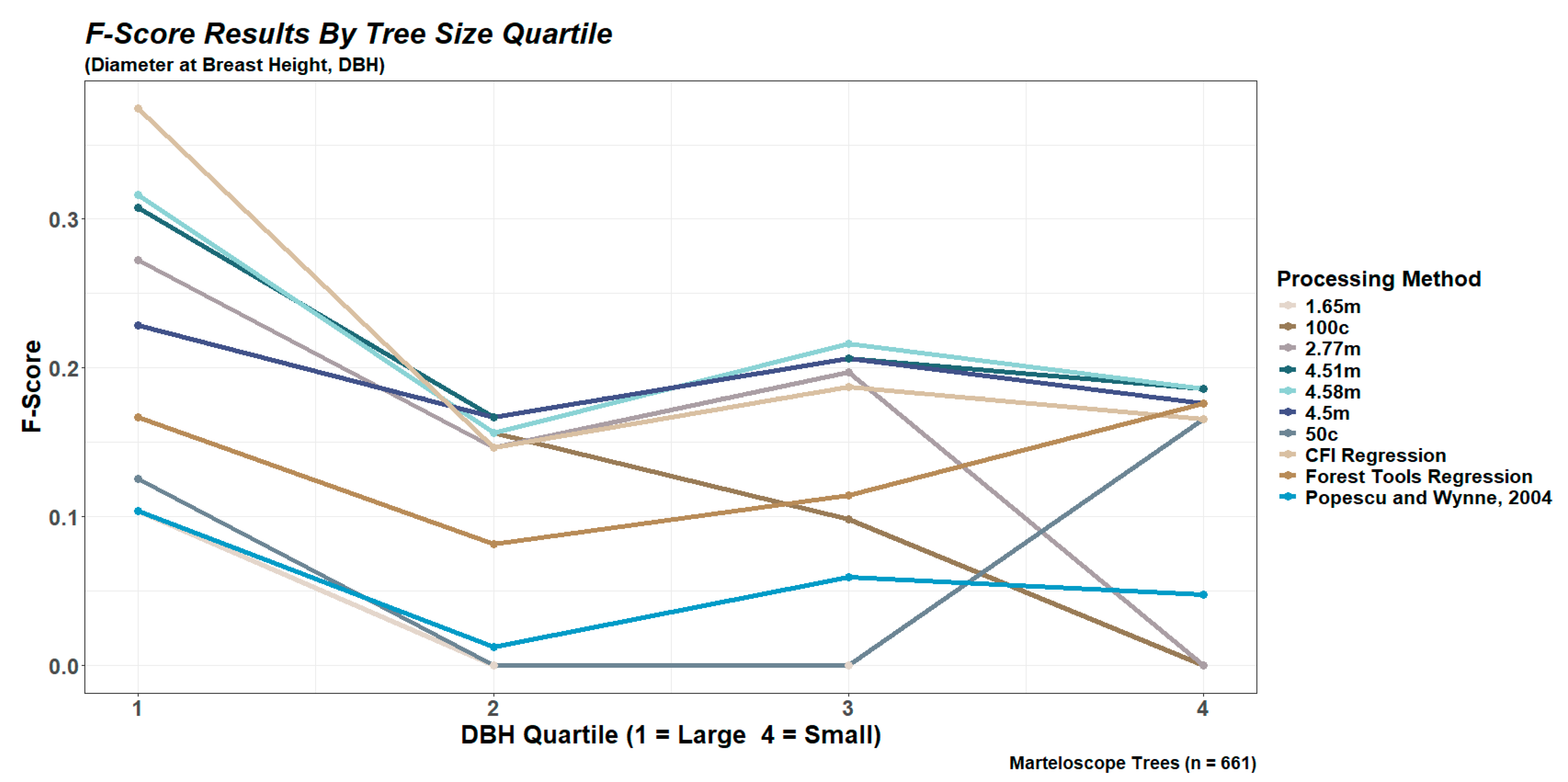
2.6.1. Performance Based on Tree Size Quartiles

For the Dudley and Burley-Demeritt study sites, the individual tree-detection accuracy was quantitatively evaluated by comparing the tree top points generated by each of the 10 window functions to the manually digitized reference tree crowns (357 for dbh and 162 for height tree classes). First, the true positive (TP, correct detection), false negative (FN, omission error), and false positive (FP, commission error) terms were calculated in ArcGIS Pro [44,52,55,75]. TP was defined as reference tree crowns which intersected a single tree top generated by the tree top detection functions. FNs were defined as reference tree crowns which did not intersect a tree top generated by the tree top detections functions. FPs were defined as reference tree crowns which were intersected by more than one tree top generated by the tree top detections functions. These calculations were used to evaluate the performance for both of the individual size classes (i.e., class 1 to 4 for both dbh and tree height) and for all reference trees. The recall (r), precision (p) and F-score terms were also calculated for each window size function, based on the following Equations (5)–(7) [76,77,78]. The F-score term, in particular, was used to compare the overall performance of each ITD method during each test as it represents the harmonic mean of the precision and recall calculations. F-score is set to a scale from 0 to 1.0, with 1.0 being a 100% accurate model.

Equation (5): Formula for recall (r) based on the true positive (TP) and false negative (FN) individual tree detection rates.

$$\mathrm{r}={\displaystyle \frac{\mathrm{T}\mathrm{P}}{(\mathrm{T}\mathrm{P}+\mathrm{F}\mathrm{N})}}$$

(5)

Equation (6): Formula for precision (p) based on the true positive (TP) and false positive (FP) individual tree detection rates.

$$\mathrm{p}={\displaystyle \frac{\mathrm{T}\mathrm{P}}{(\mathrm{T}\mathrm{P}+\mathrm{F}\mathrm{P})}}$$

(6)

Equation (7): Formula for F-score (F, weighted average precision and recall) based on the recall (r) and precision (p) individual tree detection rates.

$$\mathrm{F}=2\ast {\displaystyle \frac{\mathrm{r}\ast \mathrm{p}}{\mathrm{r}+\mathrm{p}}}$$

(7)

The same six statistical terms (TP, FN, FP, r, p, and F) were also calculated for all 10 window functions through quantitative comparison between the UAS-lidar-based tree detections and the marteloscope plot reference trees. To generate the most comparable reference data between the marteloscope plot and Lee properties, a marker-controlled watershed segmentation (MCWS) was applied to the 661 reference tree stems documented during the field sampling [79]. This process transformed the tree stem locations into defined canopy polygons, which were then clipped to the boundary of the 1 ha plot (Figure 4). TP, FN, and FP were then quantified based on the comparison between the reference tree polygons and automatically identified trees corresponding to each detection method. For this site, TPs were defined as tree crown segments which intersected a single tree stem. FN detections were defined as tree crown segments which did not intersect a tree stem point. FP detections were defined as tree crown segments which intersected more than a single tree stem. The corresponding r, p, and F-score terms were then calculated for each window function using the TP, FN, and FP rates.

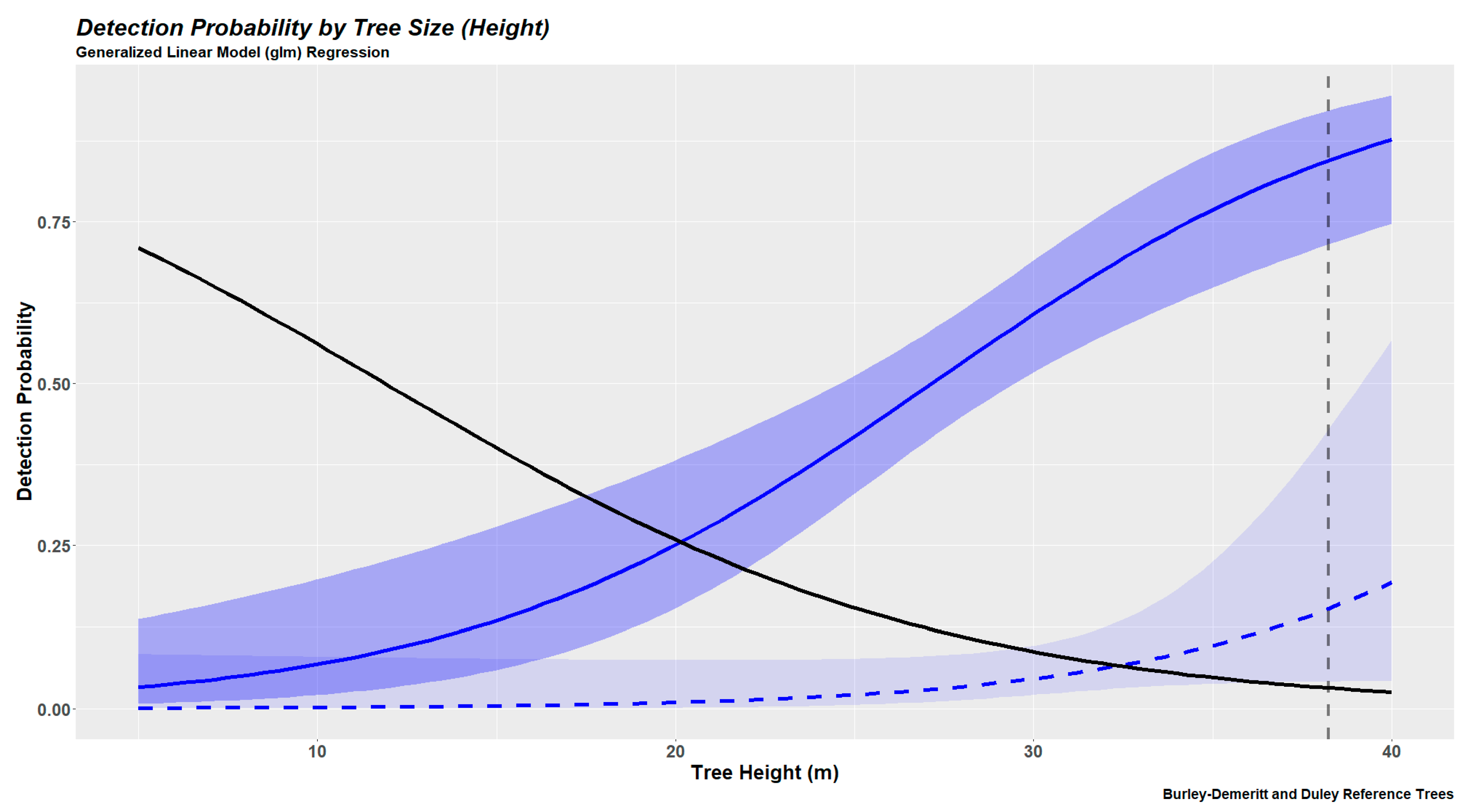
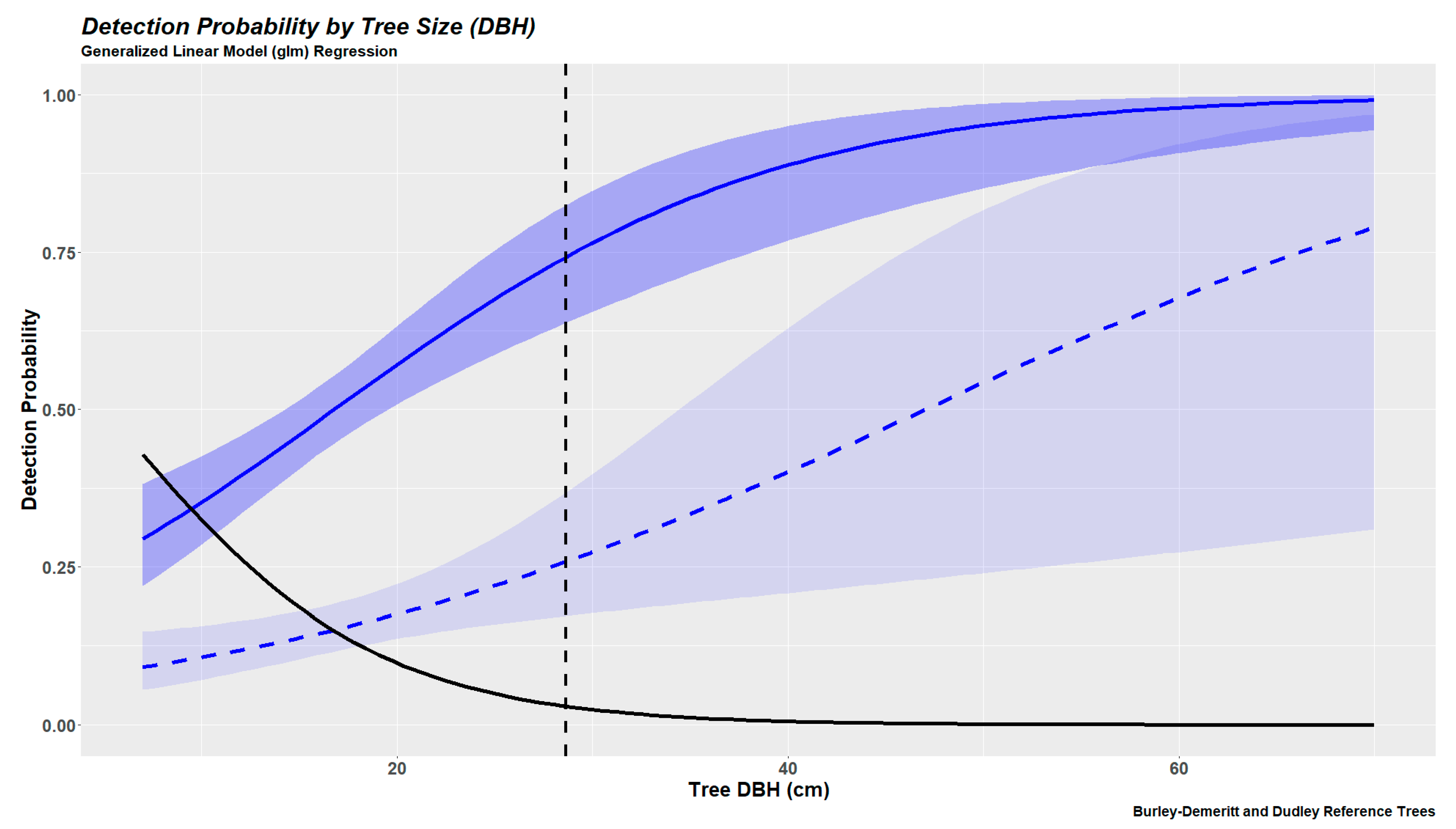
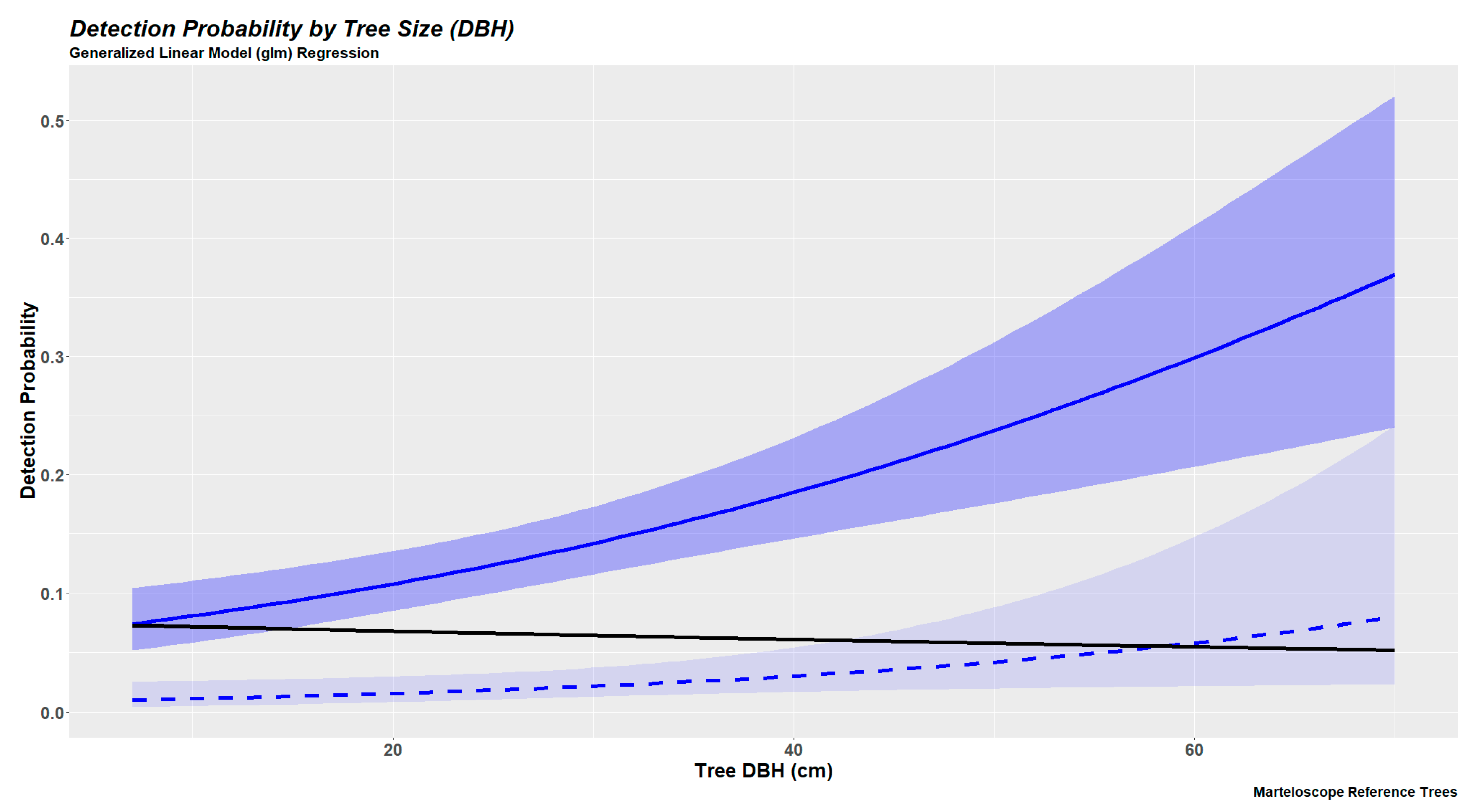
2.6.2. Tree Detection Probabilities Based on Generalized Linear Modeling

To treat the detection probability of each tree as a continuous function of either its dbh or height size, a generalized linear model was also applied to ITD records for each of the study sites [80,81]. The R generalized linear model (glm) function was used to calculate the detection (‘prediction’) probability and accompanying standard error for the most accurate window function for each study site and size metric based on the assessment of size quartiles above [82]. Here, the most accurate result was defined as the window function with the highest overall F-score. Both the TP and FP detection rates were modeled based on the glm function for this top performing method. For each study site (Lee properties or marteloscope) and size metric (dbh or height), the method with the lowest overall F-score was also modeled using the glm function. This secondary estimate was used to infer the size threshold at which any detection method would infer comparable performance.

3. Results

3.1. Tree Detection for the CFI Plots

The height measured reference trees for the Dudley and Burley-Demeritt (Lee Property) woodlands ranged in size from 12.22 m (Size 4) to 39.04 m (Size 1). The resulting F-scores for the 10 individual tree detection (ITD) methods for each of the four size classes are given in Figure 5. The methods show a greater variation in F-scores, weighted average precision and recall [78], for the largest trees (Size 1) than the smallest trees (Size 4). Size class 1 reached a maximum F-score of 0.857 (using the 4.5 m, 4.51 m, or 4.58 m fixed window function (FW)), while size class 4 reached a maximum of 0.63 (using the 4.5 m FW). Methods such as the 4.5 m FW show a good overall performance, even for the smallest class. Other methods, such as the 50 cell FW, failed to reach a 0.5 F-score for any size class. These lower accuracy methods also failed to detect many of the trees within the largest size class.

The TP, FP, and FN detections for each size class across all 10 detection methods (

Table A1. True positive (TP), false positive (FP), and false negative (FN) (from top to bottom) ITD results for each of the 10 methods as applied to the Lee property height measured reference trees. To the right: overall recall (r), precision (p), and F-score for each of the 10 ITD methods.

Method	Size 1	Size 2	Size 3	Size 4	r	p	F-Score
FW: 50 cells	0 39 1	5 33 2	6 28 7	11 24 6	0.5789	0.1507	0.2391
FW: 100 cells	12 23 5	13 17 10	18 10 13	17 1 23	0.5405	0.5405	0.5405
FW: 1.65 m	1 38 1	7 31 2	9 25 7	13 21 7	0.6383	0.2069	0.3125
FW: 4.5 m	30 4 6	24 2 14	21 0 20	19 1 21	0.6065	0.9307	0.7344
FW: 2.77 m	12 26 2	11 20 9	17 12 12	18 4 19	0.5800	0.4833	0.5273
FW: 4.58 m	30 4 6	24 2 14	21 0 20	9 1 31	0.5419	0.9231	0.6829
FW: 4.51 m	30 4 6	24 2 14	21 0 20	9 1 31	0.5419	0.9231	0.6829
Popescu Mixed Forests	27 9 4	21 8 11	16 9 16	18 5 18	0.6260	0.7257	0.6721
Forest Inventory Regression	29 0 11	18 0 22	16 0 25	4 0 37	0.4136	1.00	0.5852
ForestTools Regression	2 37 1	9 27 4	9 26 6	11 24 6	0.6458	0.2138	0.3212

), show, as expected, that the rate of omission (FN) increases for all methods as the tree height decreases. For the 4.5 m FW, specifically, which achieved the highest overall F-score (0.7344), the number of FN detections went from 6 to 21 trees. ITD methods such as the 50 cell and 1.65 m FW achieved the lowest overall F-scores at 0.2391 and 0.3125, respectively. Both maintained relatively low amounts of FN detections but also resulted in high overall amounts of commission (FP) detections. The VWF based on the forest inventory tree height to crown radius regression resulted in the highest precision, with a value of 1.0. The VWF based on the ForestTools default regression equation resulted in the highest recall (r), with a value of 0.645.

Similar trends in ITD performance for the 10 detection methods were found when applied to trees of varying dbh size classes (n = 357) across the Lee properties. The dbh size class quantiles ranged from 11.4 cm to 28.5 cm (Size 4) to 52.8 cm to 114.3 cm (Size 1). The variation in ITD results between the tree size classes is further heightened when compared to the height measured reference trees (Figure 6). For example, the largest trees (Size 1) vary in F-score from 0.8805 (4.5 m and 4.51 m FW) to 0.065 (50 cell and 1.65 m FW). For the smallest trees (Size 4), the ITD results for several detection methods ranged from 0.537 (1.65 m FW) to 0.487 (Popescu mixed forest and ForestTools VWF). Unlike for the height measured reference trees, only one detection method achieved an F-score above 0.5 for all four size classes, the 100 cell FW.

When the overall F-score is quantified for each of the ITD methods for all 357 dbh-measured reference trees, the Popescu mixed forest VWF resulted in the best performance (F-score = 0.658). The TP, FP, and FN detection rates for each of the detection methods, across each of the four dbh size classes (

Table A2. True positive (TP), false positive (FP), and false negative (FN) (from top to bottom) ITD results for each of the 10 methods as applied to the Lee property dbh measured reference trees. To the right: overall recall (r), precision (p), and F-score for each of the 10 ITD methods.

Method	Size 1	Size 2	Size 3	Size 4	r	p	F-Score
FW: 50 cells	3 84 2	9 74 6	27 51 113	30 38 22	0.627	0.218	0.324
FW: 100 cells	34 50 5	40 27 22	40 11 38	30 1 59	0.537	0.618	0.575
FW: 1.65 m	3 84 2	15 68 6	30 48 11	33 31 26	0.643	0.260	0.370
FW: 4.5 m	70 10 9	52 2 35	32 1 56	16 0 74	0.494	0.929	0.645
FW: 2.77 m	25 61 3	37 34 18	41 16 32	31 5 54	0.556	0.536	0.546
FW: 4.58 m	69 10 10	52 2 35	32 1 56	16 0 74	0.491	0.929	0.643
FW: 4.51 m	70 10 9	52 2 35	32 1 56	16 0 74	0.494	0.929	0.645
Popescu Mixed Forests	64 20 5	48 16 25	34 11 44	29 8 53	0.579	0.761	0.658
Forest Inventory Regression	68 0 21	39 0 50	18 0 71	10 0 80	0.378	1.00	0.549
ForestTools Regression	10 78 1	17 64 8	40 38 11	29 38 23	0.691	0.306	0.424

). The forest inventory tree height to crown radius regression VWF resulted in the highest precision (p = 1.0) yet failed to detect many of even the largest trees. The ForestTools default VWF resulted in the highest recall (r = 0.691).

Table 4. True positive (TP), false positive (FP), and false negative (FN) (from top to bottom) ITD results for the highest overall F-score methods as applied to the Lee property height and dbh measured reference trees. To the right: overall recall (r), precision (p), and F-score for each of the 10 ITD methods.

Height
Method	Size 1	Size 2	Size 3	Size 4	R	p	F-score
FW: 4.5 m	30 4 6	24 2 14	21 0 20	19 1 21	0.6065	0.9307	0.7344
FW: 4.58 m	30 4 6	24 2 14	21 0 20	9 1 31	0.5419	0.9231	0.6829
FW: 4.51 m	30 4 6	24 2 14	21 0 20	9 1 31	0.5419	0.9231	0.6829
DBH
Method	Size 1	Size 2	Size 3	Size 4	R	p	F-score
Popescu Mixed Forests	64 20 5	48 16 25	34 11 44	29 8 53	0.579	0.761	0.658
FW: 4.5 m	70 10 9	52 2 35	32 1 56	16 0 74	0.494	0.929	0.645
FW: 4.51 m	70 10 9	52 2 35	32 1 56	16 0 74	0.494	0.929	0.645

provides a summary of the methods which achieved the highest overall F-scores for the Lee woodlands as applied to both tree size variables (height and DBH).

3.2. Tree Detection for the Marteloscope Plot

When applied to the marteloscope plot height measured reference trees, the F-scores for each of the 10 detection methods, across all four size classes, show a general decrease in performance (Figure 7). For example, the largest of trees (Size 1, 25.8 m to 37.7 m in height) reach a maximum F-score value of 0.5, compared to a value of 0.857 above. Similarly, for the smallest size class (size class 4, 1.9 m to 11.9 m in height) the F-score statistics report a maximum overall performance of 0.222. The worst performing ITD methods (50 cell and 1.65 m FW) both failed to detect trees of intermediate size classes 2 and 3. Finally, there is a noticeable difference in overall detection performance (F-score) between methods such as the 4.5 m, 4.51 m, or 4.58 m FW and these underperforming functions.

The consistent decline in overall F-score results for each of the 10 ITD detection methods, when applied to the marteloscope plot height measured reference trees, is further confirmed in

Table A3. True positive (TP), false positive (FP), and false negative (FN) (from top to bottom) ITD results for each of the 10 methods as applied to the marteloscope plot height measured reference trees. To the right: overall recall (r), precision (p), and F-score for each of the 10 ITD methods.

Method	Size 1	Size 2	Size 3	Size 4	r	p	F-Score
FW: 50 cells	1 7 7	0 3 12	0 4 12	1 3 12	0.044	0.105	0.063
FW: 100 cells	5 2 8	2 0 13	3 0 13	0 3 13	0.175	0.667	0.278
FW: 1.65 m	1 7 7	0 3 12	0 4 12	1 3 12	0.044	0.105	0.063
FW: 4.5 m	5 1 9	3 0 12	3 0 13	2 1 13	0.217	0.867	0.347
FW: 2.77 m	5 2 8	2 1 12	3 1 12	2 1 13	0.182	0.588	0.278
FW: 4.58 m	5 1 9	3 0 12	3 0 13	0 3 13	0.217	0.867	0.347
FW: 4.51 m	5 1 9	3 0 12	3 0 13	2 1 13	0.217	0.867	0.347
Popescu Mixed Forests	0 0 0	0 0 0	0 0 0	2 0 14	0.125	1.000	0.222
Forest Inventory Regression	5 0 10	1 0 14	3 0 13	2 0 14	0.177	1.000	0.301
ForestTools Regression	2 6 7	0 3 12	1 4 11	1 3 12	0.087	0.200	0.121

. The highest overall F-scores here were achieved by the 4.5 m, 4.51 m, and 4.58 m FW, F-score = 0.347. The lowest overall performance was maintained by the 50 cell and 1.65 m FW (F-score = 0.063). Both FW resulted in low rates of TP detections, moderate rates of FP detections, and high rates of FN detection. Both the forest inventory-based VWF and Popescu mixed forest VWF achieved precision results of 1.0. The highest recall performance was achieved by the 4.5 m, 4.51 m, and 4.58 m FW (r = 0.217).

When broadened to the full set of 661 dbh measured reference trees within the marteloscope plot, the 10 ITD methods demonstrate relatively poor performance (low F-scores) for all four dbh size classes (Figure 8). The variation in results for the largest trees (Size 1) range from an F-score value of 0.374 (forest inventory regression-based VWF) to an F-score value of 0.103 (1.65 m FW and Popescu and Wynne mixed forest regression VWF). For the smallest measured trees (Size 4), the F-score value never achieved a performance greater than 0.2.

The TP, FP, and FN results for each of the 10 ITD methods for the reference trees within the marteloscope plot demonstrate considerable amounts of both commission (FP) and omission (FN) error for all methods (

Table A4. True positive (TP), false positive (FP), and false negative (FN) (from top to bottom) ITD results for each of the 10 methods as applied to the marteloscope plot reference trees. Size quartiles are defined here based on dbh size measurements. To the right: overall recall (r), precision (p), and F-score for each of the 10 ITD methods.

Method	Size 1	Size 2	Size 3	Size 4	r	p	F-Score
FW: 50 cells	11 62 92	7 37 121	9 35 121	15 30 121	0.085	0.204	0.119
FW: 100 cells	31 29 105	14 16 135	8 11 136	14 12 140	0.115	0.496	0.187
FW: 1.65 m	9 64 92	8 37 120	9 35 121	15 32 119	0.083	0.196	0.117
FW: 4.5 m	20 23 112	15 10 140	19 8 138	16 8 142	0.116	0.588	0.194
FW: 2.77 m	26 36 103	13 22 130	18 16 131	12 18 136	0.121	0.429	0.189
FW: 4.58 m	31 22 112	14 10 141	20 7 138	17 7 142	0.133	0.641	0.221
FW: 4.51 m	30 23 112	15 10 140	19 8 138	17 7 142	0.132	0.628	0.218
Popescu Mixed Forests	9 1 155	1 0 164	5 0 160	4 1 161	0.029	0.905	0.056
Forest Inventory Regression	38 6 121	13 3 149	17 1 147	15 3 148	0.128	0.865	0.223
ForestTools Regression	15 57 93	7 36 122	10 33 122	16 28 122	0.095	0.238	0.135

). The forest inventory regression-based VWF and 4.58 m FW resulted in the highest overall F-scores of 0.223 and 0.221, respectively. The Popescu and Wynne mixed forest regression-based VWF resulted in the highest precession at 0.905. The highest recall value across all ITD methods was 0.133, based on the 4.58 m FW.

Table 5. True positive (TP), false positive (FP), and false negative (FN) (from top to bottom) ITD results for the highest overall F-score methods as applied to the marteloscope plot height and dbh measured reference trees. To the right: overall recall (r), precision (p), and F-score for each of the 10 ITD methods.

Height
Method	Size 1	Size 2	Size 3	Size 4	r	p	F-score
FW: 4.5 m	5 1 9	3 0 12	3 0 13	2 1 13	0.217	0.867	0.347
FW: 4.58 m	5 1 9	3 0 12	3 0 13	0 3 13	0.217	0.867	0.347
FW: 4.51 m	5 1 9	3 0 12	3 0 13	2 1 13	0.217	0.867	0.347
DBH
Method	Size 1	Size 2	Size 3	Size 4	r	p	F-score
Forest Inventory Regression	38 6 121	13 3 149	17 1 147	15 3 148	0.128	0.865	0.223
FW: 4.58 m	31 22 112	14 10 141	20 7 138	17 7 142	0.133	0.641	0.221
FW: 4.51 m	30 23 112	15 10 140	19 8 138	17 7 142	0.132	0.628	0.218

details the ITD methods which achieved the highest overall F-scores for the marteloscope plot as applied to both tree size variables (height and DBH).

3.3. Tree Detection as a Continuous Variable (Generalized Linear Models)

The first glm regression was applied to the Burley-Demeritt and Dudley CFI plot reference trees which were measured and categorized based on their heights (Figure 9). Based on the tree-height size quartile analysis above, the top performing ITD method was based on the 4.5 m fixed window function (F-score = 0.7344). The glm function shows a steady increase in TP probability (solid blue line), with a maximum detection rate of ~0.875 for the tallest trees (height = 40 m). The FP detection probability starts to rise at tree heights over 25 m, reaching a maximum of approx. 0.23 for the tallest trees at these sites. The total detection rate, calculated by combining the TP and FP probabilities, surpassed a 90% threshold using this ITD method at approximately 38.23 m (dashed vertical black line). This 90% total detection rate is calculated to be approximately 97.9% of the maximum tree height for these sites ($H_{max}$ = 39.04 m). The worst performing ITD method, based on the 50-cell fixed window function (solid black line) shows a decreasing TP detection probability as tree height increases. The glm regression shows that at a tree height of less than approximately 20.5 m, even this worst performing method performs as well or better than any of the ITD methods.

The second glm regression was applied to the Burley-Demeritt and Dudley CFI plot reference trees which were categorized based on their dbh (all measured trees). Based on the tree dbh size quartile analysis above, the top performing ITD method was based on the Popescu and Wynne [12] mixed forest variable window function (F-score = 0.658). The glm regression function shows again a steady increase in the TP detection probability (solid blue line) as the dbh size increases (Figure 10). At tree dbh sizes larger than approximately 50 cm (44% of the maximum dbh) the TP detection probability starts to plateau. The FP detection probability shows a continual increase across all dbh sizes, reaching a detection probability just over 0.5 by 50 cm and 0.75 by 66 cm. The total detection rate threshold of 90% for this ITD method (dashed vertical black line) is estimated for trees with a roughly 28 cm dbh or larger (24.5% of maximum dbh). The worst performing ITD method, based again on the 50-cell fixed window function (solid black line) shows a sharp decrease in TP detection probability as dbh increases. At all sizes, the ITD detection probability for this method is below 0.5. Finally, this glm analysis shows that at the top performing method generates more TP detections than the worst performing method at all but the smallest (dbh) sizes.

The third glm regression analysis was applied to the marteloscope plot reference trees which were measured and categorized based on their heights (Figure 11). Based on the marteloscope tree-height size quartile analysis above, the top performing ITD method was based on the 4.5 m fixed window function (F-score = 0.347). The glm function shows an increasing TP detection probability by tree height. A maximum detection probability for the tree sizes measured at this site was estimated at just over 0.4. The FP detection probability shows just a gradual increase as tree height increases but never surpasses a rate of 0.1. The total detection rate, calculated by combining the TP and FP detection probability for this method, never reaches the 90% detection success threshold. The worst performing ITD method, based on the 50-cell fixed window function (solid black line) shows an overall poor performance, with all tree heights estimating a detection probability of less than 0.1. Additionally, this worst performing method does achieve a higher TP detection probability than the top method at any tree-height size.

The final glm regression analysis was applied to the marteloscope plot reference trees which were categorized based on their dbh (all measured trees) (Figure 12). Based on the tree (dbh) size quartile analysis above, the top performing ITD method was based on the 2015 forest inventory data height to crown radius regression (variable window function) (F-score = 0.223). The glm function shows an increasing trend in TP detection probability as dbh increases. At all dbh sizes, the TP detection probability is less than 0.4. The FP detection probability increases at a higher rate for trees with a dbh larger than 40 cm. The worst performing ITD method, based on the 1.65 m fixed window function (solid black line) shows a decreasing TP detection probability as tree (dbh) size increases. This worst performing method achieves a lower TP detection probability than the top performing method for all dbh sizes measured for this site (7 cm to 70 cm).

4. Discussion

Forests are a key component of global biodiversity and ecosystem dynamics [83]. To better understand the characteristics of forests at ecologically relevant scales, smart technologies have been increasingly leveraged throughout the 21st century under the context of precision forestry [30,84,85]. Some of these technologies include UAS and lidar sensors. In the application of UAS-lidar for precision forestry, one of the often-fundamental processing steps is to detect individual trees. Recognizing this importance, the methods, limitations, and functions of individual tree detection (ITD) have been a focus of study for over two decades [11,22,51,52]. One key insight from this research is the statistical and analytical impacts resulting from selecting a specific option from among the various ITD processing methods (algorithms and parameter combinations). To address this knowledge gap, this research focused on three considerations which should be made when using UAS-lidar to characterize complex temperate forests at the individual tree scale.

Firstly, this research quantified the relative effectiveness of 10 technologically accessible ITD methods using high-density UAS-lidar. Although many advanced algorithms exist, many practitioners lack the technical expertise, training data, or processing resources to use them. To address this objective, 10 ITD methods were applied to a diverse mixture of trees measured across three study sites [86]. These ITD methods were selected to compare numerous functions specifically designed for this region [37,44,45] or modeling process [12,44,74]. When ITD performance was analyzed based on tree size quartiles for the Lee woodlands, the 4.5 m FW detection method achieved the highest overall F-score (weighted average precision and recall, F-score = 0.7344). For this method, the F-score values ranged from 0.857 to 0.6333 for tree height size classes 1 (large) through 4 (small), respectively. For the dbh size classes, the F-scores for this same method ranged from 0.8805 to 0.3018, sizes 1 through 4 (F-score = 0.645 overall). These results suggest that there is a greater variance in F-scores (overall performance) for trees varying in dbh size classes than height size classes. Zaforemska et al. [44] achieved an average F-score of 0.802, across 1 mixed (2-species) and five single species plots. Fraser et al. [37] reported an overall F-score of 0.785 based on the same 4.5 m FW detection method, as applied to a similar composition of tree species (although with less tree size diversity). Xu et al. [87] reported F-scores ranging from 0.607 to 0.737 for detecting trees within their more complex, mixed broadleaf, stand. Yin et al. [36] reported an F-score of 0.630 using UAS-lidar to detect individual mangrove trees. Based on the statistical comparison between the UAS-lidar derived tree detections and the field-measured reference trees, a VWF based on a regression equation calculated from a forest inventory-based crown radius to tree height, followed by a 4.58 m FW method resulted in the highest overall F-scores (0.223 and 0.221, respectively). The 4.5 m FW performed relatively well but only achieved an F-score of 0.194 when applied to the marteloscope plot. These low F-score results suggest that even at higher point cloud densities, processing and analyzing UAS-lidar data as 2D raster data (i.e., canopy height models, CHM) are ineffective for use in complex, multi-layered canopies.

Secondly, this research was to determine which, and to what extent, specific sizes of trees were being under- or over-represented in UAS-lidar-based ITD analyses. A combination of the tree size quartile analysis and the generalized linear model (glm, i.e., continuous) analyses were used to satisfy this objective. The tree size quartile analysis validated that the largest trees for both height and dbh (size class 1) consistently showed a greater detection performance (F-score) when compared to the smallest trees (size class 4). Such results are consistent with other literature based on UAS-lidar and complex forests [35,87]. Additionally, the detection rate for largest size class was not universally higher for all ITD methods, suggesting some methods did not accurately reflect the tree sizes present in this landscape. The glm regression analyses determined that, when analyzed based on a tree height gradient, only the tallest trees (those taller than 38 m) achieved an overall detection probability greater than 90%. The TP detection probability reached a maximum of 0.875 (87.5%) for the Burley-Demeritt and Dudley reference trees. Trees less than 50% of the maximum recorded tree height (39.04 m) resulted in a detection probability less than 50% based on this same ITD method. Additionally, trees with heights less than 20 m (approx. 50% of the maximum recorded tree height) had an equal or lesser chance of detection using any of the 10 ITD methods. Goldbergs et al. [88] provided evidence that the detection of dominant and co-dominant trees would achieve higher accuracies (~70%) compared to suppressed trees (<35%), following the conventional understanding of remote-sensing applications. When applied to trees across a range of dbh sizes, the ITD probability (TP detection probability) started to plateau at rates above 90% for the largest one-third of tree sizes. A 90% overall detection threshold was reached at dbh sizes greater than 28 cm (24.5% of the maximum recorded dbh for these sites). Only the smallest 20% of trees resulted in a detection probability less than 50% during this analysis. These results agree with raster-based local maxima detection method applied in Torresan et al. [89], which estimated a notably lower detection probability for small diameter trees within multi-layered mixed forests.

Thirdly, current day practitioners of UAS-lidar also face a challenge in that lidar point densities have increased considerably in recent years, leading to discrepancies between current data resolutions and conventional processing recommendations. Foundational studies on UAS-lidar ITD methods within the last 10 years have defined ‘high density’ point clouds at 5 to 50 ${\mathrm{p}\mathrm{t}\mathrm{s}/\mathrm{m}}^2$ [46]. Modern lidar sensors can capture point densities at an order of magnitude higher than such studies (e.g., up to and exceeding 1000 ${\mathrm{p}\mathrm{t}\mathrm{s}/\mathrm{m}}^2$) [44,47,48,90], making the direct adoption of historically validated methods less appropriate. While this study bases its results on UAS-lidar data with a point density greater than 800 ${\mathrm{p}\mathrm{t}\mathrm{s}/\mathrm{m}}^2$, in most cases the reliance on 2D CHM-based methods for ITD proves to be insufficient in detecting trees within complex forests. For example, each test and method reported the low detection probability of small dbh and shorter trees within these multi-layered, complex, forests.

Speaking to the practicality of the currently tested 10 ITD methods, the three VWF methods failed to notably outperform the seven FW methods tested here. During both of the dbh-based tree size analyses (quartile and glm regression) the top performing method was based on a VWF regression function; however, the overall F-scores were only slightly higher than the FW methods. Despite the comparable performance, both the VWF based on the default ForestTools parameters [12,74] and the 2015 forest inventory regression equation [37,56] took hours longer to finish processing. The VWF based on the Popescu and Wynne [12] mixed forest regression equation required days longer to finish processing, when compared to the processing time for the FW methods. Further highlighting this difference in processing performance, an 11th ITD function, based on a regression equation calculated from the regression between digitized tree crown width and tree heights for the Lee properties was initially investigated [37,91,92]. The processing time for this method was estimated to take more than a month, based on an average completion rate of approximately 1% per day for the Burley-Demeritt study site. Such processing time requirements make these methods impractical for operational use.

The results detail the findings of applying 10 unique ITD methods across a range of tree height and dbh size classes. For practitioners looking to adopt such methods for their own precision forestry projects, such information provides a basis for methodological decision making. This decision-making ability can then be better paired with other considerations of practicality and accessibility. For example, UAS-lidar ITD methods are not limited to CHM techniques. Voxel [93,94,95] or point cloud-based segmentation techniques [96,97,98,99] are also available but require additional technical expertise. The fusion of structural metrics and image-based data (spectral information) are also a viable option [100,101,102] for ITD. Additionally, sensor and site independent techniques, built on the foundation of large amounts of individual tree annotations (training data) are starting to become available [90].

Trees of diverse height and dbh size classes are important components of New England temperate forests and other complex forests around the world [39,40,86,103]. More research is needed to ensure that the performance and transferability of ITD methods are comprehensively detailed and understood. This may necessitate similar studies focused on alternate forest types or densities (stems/ha).

References

- Kershaw, J.A.; Ducey, M.J.; Beers, T.W.; Husch, B. Forest Mensuration, 5th ed.; John Wiley and Sons Ltd.: Hoboken, NJ, USA, 2016. [Google Scholar]
- Burkhart, H.E.; Avery, T.E.; Bullock, B.P. Forest Measurements, 6th ed.; Waveland Press, INC: Long Grove, IL, USA, 2019; ISBN 1-4786-3618-1. [Google Scholar]
- del Río, M.; Pretzsch, H.; Alberdi, I.; Bielak, K.; Bravo, F.; Brunner, A.; Condés, S.; Ducey, M.J.; Fonseca, T.; von Lüpke, N.; et al. Characterization of Mixed Forests. In Dynamics, Silviculture and Management of Mixed Forests; Bravo-Oviedo, A., Pretzsch, H., del Río, M., Eds.; Springer International Publishing: Cham, Switzerland, 2018; pp. 27–71. ISBN 978-3-319-91953-9. [Google Scholar]
- Corte, A.P.D.; Souza, D.V.; Rex, F.E.; Sanquetta, C.R.; Mohan, M.; Silva, C.A.; Zambrano, A.M.A.; Prata, G.; Alves de Almeida, D.R.; Trautenmüller, J.W.; et al. Forest Inventory with High-Density UAV-Lidar: Machine Learning Approaches for Predicting Individual Tree Attributes. Comput. Electron. Agric. 2020, 179, 105815. [Google Scholar] [CrossRef]
- Spurr, S.H. Aerial Photographs in Forestry, 1st ed.; Ronald Press, Co.: New York, NY, USA, 1948; 340p. [Google Scholar]
- Avery, T.E. Forester’s Guide To Aerial Photo Interpretation; USDA Forest Service: Washington, DC, USA, 1969; 40p. [Google Scholar]
- Lillesand, T.; Kiefer, R.W.; Chipman, J. Remote Sensing and Image Interpretation, 7th ed.; John Wiley and Sons Ltd.: Hoboken, NJ, USA, 2015; ISBN 978-1-118-34328-9. [Google Scholar]
- Sexton, J.O.; Bax, T.; Siqueira, P.; Swenson, J.J.; Hensley, S. A Comparison of Lidar, Radar, and Field Measurements of Canopy Height in Pine and Hardwood Forests of Southeastern North America. For. Ecol. Manag. 2009, 257, 1136–1147. [Google Scholar] [CrossRef]
- Holopainen, M.; Vastaranta, M.; Karjalainen, M.; Karila, K.; Kaasalainen, S.; Honkavaara, E.; Hyyppä, J. Forest Inventory Attribute Estimation Using Airborne Laser Scanning, Aerial Stereo Imagery, Radargrammetry and Interferometry-Finnish Experiences of the 3d Techniques. ISPRS Ann. Photogramm. Remote Sens. Spat. Inf. Sci. 2015, 2, 63–69. [Google Scholar] [CrossRef]
- Chen, Y.; Hakala, T.; Karjalainen, M.; Feng, Z.; Tang, J.; Litkey, P.; Kukko, A.; Jaakkola, A.; Hyyppä, J. UAV -Borne Profiling Radar for Forest Research. Remote Sens. 2017, 9, 58. [Google Scholar] [CrossRef]
- Vierling, K.T.; Vierling, L.A.; Gould, W.A.; Martinuzzi, S.; Clawges, R.M. Lidar: Shedding New Light on Habitat Characterization and Modeling. Front. Ecol. Environ. 2008, 6, 90–98. [Google Scholar] [CrossRef]
- Popescu, S.C.; Wynne, R.H. Seeing the Trees in the Forest: Using Lidar and Multispectral Data Fusion with Local Filtering and Variable Window Size for Estimating Tree Height. Photogramm. Eng. Remote Sens. 2004, 70, 589–604. [Google Scholar] [CrossRef]
- Su, Y.; Ma, Q.; Guo, Q. Fine-Resolution Forest Tree Height Estimation across the Sierra Nevada through the Integration of Spaceborne LiDAR, Airborne LiDAR, and Optical Imagery. Int. J. Digit. Earth 2017, 10, 307–323. [Google Scholar] [CrossRef]
- Rosette, J.; Suarez, J.; North, P.; Los, S. Forestry Applications for Satellite Lidar Remote Sensing. Photogramm. Eng. Remote Sens. 2011, 77, 271–279. [Google Scholar] [CrossRef]
- Renslow, M. Manual of Airborne Topographic Lidar; ASPRS: Bethesda, MD, USA, 2013; ISBN 1-57083-097-5. [Google Scholar]
- Vauhkonen, J.; Maltamo, M.; McRoberts, R.E.; Næsset, E. Introduction to Forestry Applications of Airborne Laser Scanning. In Forestry Applications of Airborne Laser Scanning: Concepts and Case Studies; Maltamo, M., Næsset, E., Vauhkonen, J., Eds.; Springer: Dordrecht, The Netherlands, 2014; pp. 1–16. ISBN 978-94-017-8663-8. [Google Scholar]
- Donager, J.J.; Sankey, T.T.; Sankey, J.B.; Sanchez Meador, A.J.; Springer, A.E.; Bailey, J.D. Examining Forest Structure with Terrestrial Lidar: Suggestions and Novel Techniques Based on Comparisons Between Scanners and Forest Treatments. Earth Space Sci. 2018, 5, 753–776. [Google Scholar] [CrossRef]
- Calders, K.; Adams, J.; Armston, J.; Bartholomeus, H.; Bauwens, S.; Bentley, L.P.; Chave, J.; Danson, F.M.; Demol, M.; Disney, M.; et al. Terrestrial Laser Scanning in Forest Ecology: Expanding the Horizon. Remote Sens. Environ. 2020, 251, 112102. [Google Scholar] [CrossRef]
- Dassot, M.; Constant, T.; Fournier, M. The Use of Terrestrial LiDAR Technology in Forest Science: Application Fields, Benefits and Challenges. Ann. For. Sci. 2011, 68, 959–974. [Google Scholar] [CrossRef]
- Di Stefano, F.; Chiappini, S.; Gorreja, A.; Balestra, M.; Pierdicca, R. Mobile 3D Scan LiDAR: A Literature Review. Geomat. Nat. Hazards Risk 2021, 12, 2387–2429. [Google Scholar] [CrossRef]
- Heo, H.K.; Lee, D.K.; Park, J.H.; Thorne, J.H. Estimating the Heights and Diameters at Breast Height of Trees in an Urban Park and along a Street Using Mobile LiDAR. Landsc. Ecol. Eng. 2019, 15, 253–263. [Google Scholar] [CrossRef]
- Wallace, L.; Lucieer, A.; Watson, C.; Turner, D. Development of a UAV-LiDAR System with Application to Forest Inventory. Remote Sens. 2012, 4, 1519–1543. [Google Scholar] [CrossRef]
- Hu, T.; Sun, X.; Su, Y.; Guan, H.; Sun, Q.; Kelly, M.; Guo, Q. Development and Performance Evaluation of a Very Low-Cost UAV-Lidar System for Forestry Applications. Remote Sens. 2021, 13, 77. [Google Scholar] [CrossRef]
- Beland, M.; Parker, G.; Sparrow, B.; Harding, D.; Chasmer, L.; Phinn, S.; Antonarakis, A.; Strahler, A. On Promoting the Use of Lidar Systems in Forest Ecosystem Research. For. Ecol. Manag. 2019, 450, 117484. [Google Scholar] [CrossRef]
- Pilarska, M.; Ostrowski, W.; Bakuła, K.; Górski, K.; Kurczyński, Z. The Potential of Light Laser Scanners Developed for Unmanned Aerial Vehicles—The Review and Accuracy. Int. Arch. Photogramm. Remote Sens. Spat. Inf. Sci.-ISPRS Arch. 2016, 42, 87–95. [Google Scholar] [CrossRef]
- Nitoslawski, S.A.; Wong-Stevens, K.; Steenberg, J.W.N.; Witherspoon, K.; Nesbitt, L.; Konijnendijk van den Bosch, C.C. The Digital Forest: Mapping a Decade of Knowledge on Technological Applications for Forest Ecosystems. Earths Future 2021, 9, 1–28. [Google Scholar] [CrossRef]
- Corte, A.P.D.; Rex, F.E.; de Almeida, D.R.A.; Sanquetta, C.R.; Silva, C.A.; Moura, M.M.; Wilkinson, B.; Zambrano, A.M.A.; da Cunha Neto, E.M.; Veras, H.F.P.; et al. Measuring Individual Tree Diameter and Height Using Gatoreye High-Density UAV-Lidar in an Integrated Crop-Livestock-Forest System. Remote Sens. 2020, 12, 863. [Google Scholar] [CrossRef]
- Brede, B.; Lau, A.; Bartholomeus, H.M.; Kooistra, L. Comparing RIEGL RiCOPTER UAV LiDAR Derived Canopy Height and DBH with Terrestrial LiDAR. Sensors 2017, 17, 2371. [Google Scholar] [CrossRef]
- Alsadik, B.; Remondino, F. Flight Planning for LiDAR-Based UAS Mapping Applications. ISPRS Int. J. Geoinf. 2020, 9, 378. [Google Scholar] [CrossRef]
- Fraser, B.T.; Bunyon, C.L.; Reny, S.; Lopez, I.S.; Congalton, R.G. Analysis of Unmanned Aerial System (UAS) Sensor Data for Natural Resource Applications: A Review. Geographies 2022, 2, 303–340. [Google Scholar] [CrossRef]
- Liu, K.; Shen, X.; Cao, L.; Wang, G.; Cao, F. Estimating Forest Structural Attributes Using UAV-LiDAR Data in Ginkgo Plantations. ISPRS J. Photogramm. Remote Sens. 2018, 146, 465–482. [Google Scholar] [CrossRef]
- Zhou, X.; Ma, K.; Sun, H.; Li, C.; Wang, Y. Estimation of Forest Stand Volume in Coniferous Plantation from Individual Tree Segmentation Aspect Using UAV-LiDAR. Remote Sens. 2024, 16, 2736. [Google Scholar] [CrossRef]
- Liu, L.; Lim, S.; Shen, X.; Yebra, M. A Hybrid Method for Segmenting Individual Trees from Airborne Lidar Data. Comput. Electron. Agric. 2019, 163, 104871. [Google Scholar] [CrossRef]
- Zhen, Z.; Quackenbush, L.J.; Zhang, L. Trends in Automatic Individual Tree Crown Detection and Delineation-Evolution of LiDAR Data. Remote Sens. 2016, 8, 333. [Google Scholar] [CrossRef]
- Fraser, B.T.; Congalton, R.G. Estimating Primary Forest Attributes and Rare Community Characteristics Using Unmanned Aerial Systems (UAS): An Enrichment of Conventional Forest Inventories. Remote Sens. 2021, 13, 2971. [Google Scholar] [CrossRef]
- Yin, D.; Wang, L. Individual Mangrove Tree Measurement Using UAV-Based LiDAR Data: Possibilities and Challenges. Remote Sens. Environ. 2019, 223, 34–49. [Google Scholar] [CrossRef]
- You, H.; Liu, Y.; Lei, P.; Qin, Z.; You, Q. Segmentation of Individual Mangrove Trees Using UAV-Based LiDAR Data. Ecol. Inform. 2023, 77, 102200. [Google Scholar] [CrossRef]
- Liang, X.; Wang, Y.; Pyörälä, J.; Lehtomäki, M.; Yu, X.; Kaartinen, H.; Kukko, A.; Honkavaara, E.; Issaoui, A.E.I.; Nevalainen, O.; et al. Forest in Situ Observations Using Unmanned Aerial Vehicle as an Alternative of Terrestrial Measurements. For. Ecosyst. 2019, 6, 20. [Google Scholar] [CrossRef]
- Braun, E.L. Deciduous Forests of Eastern North America, 1st ed.; Echo Point Books & Media, LLC: Brattleboro, VT, USA, 2023; ISBN 1648373119. [Google Scholar]
- Yahner, R.H. Eastern Deciduous Forest, 2nd ed.; Univ of Minnesota Press: Minneapolis, MN, USA, 2000; ISBN 9780816633609. [Google Scholar]
- Puliti, S.; Granhus, A. Drone Data for Decision Making in Regeneration Forests: From Raw Data to Actionable Insights. J. Unmanned Veh. Syst. 2021, 9, 45–58. [Google Scholar] [CrossRef]
- Zaforemska, A.; Xiao, W.; Gaulton, R. Individual Tree Detection from Uav Lidar Data in a Mixed Species Woodland. Int. Arch. Photogramm. Remote Sens. Spat. Inf. Sci.-ISPRS Arch. 2019, 42, 657–663. [Google Scholar] [CrossRef]
- Gu, J.; Grybas, H.; Congalton, R.G. A Comparison of Forest Tree Crown Delineation from Unmanned Aerial Imagery Using Canopy Height Models vs. Spectral Lightness. Forests 2020, 11, 605. [Google Scholar] [CrossRef]
- Reny, S.A. The Estimation of Forest Inventory Biometrics Using UAS-Lidar. Master’s Thesis, University of New Hampshire, Durham, NH, USA, 2023. [Google Scholar]
- Wallace, L.; Lucieer, A.; Watson, C.S. Evaluating Tree Detection and Segmentation Routines on Very High Resolution UAV LiDAR Ata. IEEE Trans. Geosci. Remote Sens. 2014, 52, 7619–7628. [Google Scholar] [CrossRef]
- Iheaturu, C.J.; Hepner, S.; Batchelor, J.L.; Agonvonon, G.A.; Akinyemi, F.O.; Wingate, V.R.; Ifejika Speranza, C. Integrating UAV LiDAR and Multispectral Data to Assess Forest Status and Map Disturbance Severity in a West African Forest Patch. Ecol. Inform. 2024, 84, 102876. [Google Scholar] [CrossRef]
- Deng, S.; Jing, S.; Zhao, H. A Hybrid Method for Individual Tree Detection in Broadleaf Forests Based on UAV-LiDAR Data and Multistage 3D Structure Analysis. Forests 2024, 15, 1043. [Google Scholar] [CrossRef]
- Ferreira, M.P.; Martins, G.B.; de Almeida, T.M.H.; da Silva Ribeiro, R.; da Veiga Júnior, V.F.; da Silva Rocha Paz, I.; de Siqueira, M.F.; Kurtz, B.C. Estimating Aboveground Biomass of Tropical Urban Forests with UAV-Borne Hyperspectral and LiDAR Data. Urban. For. Urban. Green. 2024, 96, 128362. [Google Scholar] [CrossRef]
- Kanaskie, C.R.; Routhier, M.R.; Fraser, B.T.; Congalton, R.G.; Ayres, M.P.; Garnas, J.R. Early Detection of Southern Pine Beetle Attack by UAV-Collected 2 Multispectral Imagery. Remote Sens. 2024, 16, 2608. [Google Scholar] [CrossRef]
- Nevalainen, O.; Honkavaara, E.; Tuominen, S.; Viljanen, N.; Hakala, T.; Yu, X.; Hyyppä, J.; Saari, H.; Pölönen, I.; Imai, N.N.; et al. Individual Tree Detection and Classification with UAV-Based Photogrammetric Point Clouds and Hyperspectral Imaging. Remote Sens. 2017, 9, 185. [Google Scholar] [CrossRef]
- Hirschmugl, M.; Ofner, M.; Raggam, J.; Schardt, M. Single Tree Detection in Very High Resolution Remote Sensing Data. Remote Sens. Environ. 2007, 110, 533–544. [Google Scholar] [CrossRef]
- Liu, Y.; You, H.; Tang, X.; You, Q.; Huang, Y.; Chen, J. Study on Individual Tree Segmentation of Different Tree Species Using Different Segmentation Algorithms Based on 3D UAV Data. Forests 2023, 14, 1327. [Google Scholar] [CrossRef]
- Rollinson, C.R.; Alexander, M.R.; Dye, A.W.; Moore, D.J.P.; Pederson, N.; Trouet, V. Climate Sensitivity of Understory Trees Differs from Overstory Trees in Temperate Mesic Forests. Ecology 2021, 102, e03264. [Google Scholar] [CrossRef] [PubMed]
- Fraser, B.; Congalton, R.G. A Comparison of Methods for Determining Forest Composition from High-Spatial Resolution Remotely Sensed Imagery. Forests 2021, 12, 1290. [Google Scholar] [CrossRef]
- de Oliveira, L.F.R.; Lassiter, H.A.; Wilkinson, B.; Whitley, T.; Ifju, P.; Logan, S.R.; Peter, G.F.; Vogel, J.G.; Martin, T.A. Moving to Automated Tree Inventory: Comparison of Uas-Derived Lidar and Photogrammetric Data with Manual Ground Estimates. Remote Sens. 2021, 13, 72. [Google Scholar] [CrossRef]
- Eisenhaure, S. Burley-Demeritt and Dudley Lot Management and Operations Plan Original 2010—Update 2016; Office of Woodlands and Natural Areas, Univeristy of New Hampshire: Durham, NH, USA, 2016. [Google Scholar]
- Eisenhaure, S. Assessment of Natural Resources and Uses at the Woodman Horticultural Farm; Office of Woodlands and Natural Areas, Univeristy of New Hampshire: Durham, NH, USA, 2013. [Google Scholar]
- EOS Arrow 100 RTK GNSS. Available online: https://eos-gnss.com/product/arrow-series/arrow-200/?gclid=Cj0KCQjw2tCGBhCLARIsABJGmZ47-nIPNrAuu7Xobgf3P0HGlV4mMLHHWZz25lyHM6UuI_pPCu7b2gMaAukeEALw_wcB (accessed on 10 March 2025).
- Marshall, D.D.; Iles, K.; Bell, J.F. Using a Large-Angle Gauge to Select Trees for Measurement in Variable Plot Sampling. Can. J. For. Res. 2004, 34, 840–845. [Google Scholar] [CrossRef]
- Derks, J.; Krumm, F.; Krau, D. GUIDELINES FOR ESTABLISHING I+ Marteloscopes; European Forest Institue: Joensuu, Finland, 2020. [Google Scholar]
- Cosyns, H.; Joa, B.; Mikoleit, R.; Krumm, F.; Schuck, A.; Winkel, G.; Schulz, T. Resolving the Trade-off between Production and Biodiversity in Integrated Forest Management: Comparing Selection Practices of Foresters and Conservationists. Biodivers. Conserv. 2020, 29, 3717–3737. [Google Scholar] [CrossRef]
- O’Brien, L.; Derks, J.; Schuck, A. The Use of Marteloscopes in Science; A Review of Past Research and Suggestions for Further Application; European Forest Institue: Joensuu, Finland, 2022. [Google Scholar]
- Derks, J.; Schuck, A.; O’Brien, L. Forestry Training WITH I+ MARTELOSCOPES; Integrate Network; European Forest Institue: Joensuu, Finland, 2022. [Google Scholar]
- Schuck, A.; Krumm, F.; Kraus, D. Integrate+ Marteloscopes Description of Parameters and Assessment Procedures; European Forest Institue: Joensuu, Finland, 2015. [Google Scholar]
- Stroner, M.; Urban, R.; Linkova, L. A New Method for UAV Lidar Precision Testing Used for the Evaluation of an Affordable DJI ZENMUS L1 Scanner. Remote Sens. 2021, 13, 4811. [Google Scholar] [CrossRef]
- Fraser, B.T.; Congalton, R.G. Issues in Unmanned Aerial Systems (UAS) Data Collection of Complex Forest Environments. Remote Sens. 2018, 10, 908. [Google Scholar] [CrossRef]
- Roussel, J.-R.; Goodbody, T.R.H.; Tompalski, P. The LidR Package. Available online: https://r-lidar.github.io/lidRbook/ (accessed on 12 June 2024).
- Roussel, J.; Auty, D. Airborne LiDAR Data Manipulation and Visualization for Forestry Applications; R Package Version 4.2.0. 2024. Available online: https://cran.r-project.org/package=lidR (accessed on 5 January 2025).
- Roussel, J.R.; Auty, D.; Coops, N.C.; Tompalski, P.; Goodbody, T.R.H.; Meador, A.S.; Bourdon, J.F.; de Boissieu, F.; Achim, A. LidR: An R Package for Analysis of Airborne Laser Scanning (ALS) Data. Remote Sens. Environ. 2020, 251, 112061. [Google Scholar] [CrossRef]
- R Core Team. R: A Language and Environment for Statistical Computing; R Foundation for Statistical Computing: Vienna, Austria, 2021. [Google Scholar]
- Zhang, W.; Qi, J.; Wan, P.; Wang, H.; Xie, D.; Wang, X.; Yan, G. An Easy-to-Use Airborne LiDAR Data Filtering Method Based on Cloth Simulation. Remote Sens. 2016, 8, 501. [Google Scholar] [CrossRef]
- Oliver, M.A.; Webster, R. Kriging: A Method of Interpolation for Geographical Information Systems. Int. J. Geogr. Inf. Syst. 1990, 4, 313–332. [Google Scholar] [CrossRef]
- Olea, R.A. Optimal Contour Mapping Using Universal Kriging. J. Geophys. Res. 1974, 79, 695–702. [Google Scholar] [CrossRef]
- Plowright, A.; Roussel, J.-R. ForestTools: Tools for Analyzing Remote Sensing Forest Data. 2024. Available online: https://cran.r-project.org/web/packages/ForestTools/index.html (accessed on 5 January 2025).
- Mohan, M.; Silva, C.A.; Klauberg, C.; Jat, P.; Catts, G.; Cardil, A.; Hudak, A.T.; Dia, M. Individual Tree Detection from Unmanned Aerial Vehicle (UAV) Derived Canopy Height Model in an Open Canopy Mixed Conifer Forest. Forests 2017, 8, 340. [Google Scholar] [CrossRef]
- Ke, Y.; Quackenbush, L.J. A Review of Methods for Automatic Individual Tree-Crown Detection and Delineation from Passive Remote Sensing. Int. J. Remote Sens. 2011, 32, 4725–4747. [Google Scholar] [CrossRef]
- Li, W.; Guo, Q.; Jakubowski, M.K.; Kelly, M. A New Method for Segmenting Individual Trees from the Lidar Point Cloud. Photogramm. Eng. Remote Sens. 2012, 78, 75–84. [Google Scholar] [CrossRef]
- Goos, G.; Hartmanis, J.; Van, J.; Board, L.E.; Hutchison, D.; Kanade, T.; Kittler, J.; Kleinberg, J.M.; Mattern, F.; Zurich, E.; et al. LNCS 3408—Advances in Information Retrieval. In Proceedings of the Advances in Information Retrieval; Losada, D.E., Fernandez-Luna, J.M., Eds.; Springer: Santiago de Compostela, Spain, 2005; pp. 1–571. [Google Scholar]
- Beucher, S.; Meyer, F. The Morphological Approach to Segmentation: The Watershed Transformation. In Mathematical Morphology in Image Processing; CRC Press: Boca Raton, FL, USA, 1992; p. 552. ISBN 9781315214610. [Google Scholar]
- Hosmer, D.W.; Lemeshow, S. Applied Logistic Regression, Wiley Series in Probability and Statistics; 2nd ed.; Wiley-Interscience Publication: New York, NY, USA, 2000; ISBN 978-0471356325. [Google Scholar]
- Everitt, B.S.; Hothorn, T. A Handbook of Statistical Analyses Using R, 2nd ed.; CRC Press: Boca Raton, FL, USA, 2010; ISBN 978-1-4200-7933-3. [Google Scholar]
- UCLA: Statistical Consulting Group Logit Regression|R Data Analysis Examples. Available online: https://stats.oarc.ucla.edu/r/dae/logit-regression/ (accessed on 5 January 2025).
- Kashian, D.M.; Zak, D.R.; Barnes, B.V.; Spurr, S.H. Forest Ecology, 5th ed.; Wiley: Hoboken, NJ, USA, 2023; ISBN 978-1119476085. [Google Scholar]
- Goodbody, T.R.H.; Coops, N.C.; Marshall, P.L.; Tompalski, P.; Crawford, P. Unmanned Aerial Systems for Precision Forest Inventory Purposes: A Review and Case Study. For. Chron. 2017, 93, 71–81. [Google Scholar] [CrossRef]
- Taylor, S.E.; McDonald, T.P.; Veal, M.W.; Corley, F.W.; Grift, T.E. Precision Forestry: Operational Tactics for Today and Tomorrow. In Proceedings of the 25th Annual Meeting of the Council of Forest Engineers, Auburn, AL, USA, 16–20 June 2002; Volume 6. [Google Scholar]
- Ehbrecht, M.; Seidel, D.; Annighöfer, P.; Kreft, H.; Köhler, M.; Zemp, D.C.; Puettmann, K.; Nilus, R.; Babweteera, F.; Willim, K.; et al. Global Patterns and Climatic Controls of Forest Structural Complexity. Nat. Commun. 2021, 12, 519. [Google Scholar] [CrossRef]
- Xu, W.; Deng, S.; Liang, D.; Cheng, X. A Crown Morphology-Based Approach to Individual Tree Detection in Subtropical Mixed Broadleaf Urban Forests Using UAV Lidar Data. Remote Sens. 2021, 13, 1278. [Google Scholar] [CrossRef]
- Goldbergs, G.; Maier, S.W.; Levick, S.R.; Edwards, A. Efficiency of Individual Tree Detection Approaches Based on Light-Weight and Low-Cost UAS Imagery in Australian Savannas. Remote Sens. 2018, 10, 161. [Google Scholar] [CrossRef]
- Torresan, C.; Carotenuto, F.; Chiavetta, U.; Miglietta, F.; Zaldei, A.; Gioli, B. Individual Tree Crown Segmentation in Two-Layered Dense Mixed Forests from Uav Lidar Data. Drones 2020, 4, 10. [Google Scholar] [CrossRef]
- Wielgosz, M.; Puliti, S.; Xiang, B.; Schindler, K.; Astrup, R. SegmentAnyTree: A Sensor and Platform Agnostic Deep Learning Model for Tree Segmentation Using Laser Scanning Data. Remote Sens. Environ. 2024, 313, 114367. [Google Scholar] [CrossRef]
- Minor, C.O. Stem-Crown Diameter Relations in Southern Pine. J. For. 1951, 59, 490–493. [Google Scholar]
- Bonnor, G.M. A Tree Volume Table for Red Pine by Crown Width and Height. For. Chron. 1964, 40, 339–346. [Google Scholar] [CrossRef]
- Wang, C.; Luo, S.; Xi, X.; Nie, S.; Ma, D.; Huang, Y. Influence of Voxel Size on Forest Canopy Height Estimates Using Full-Waveform Airborne LiDAR Data. For. Ecosyst. 2020, 7, 31. [Google Scholar] [CrossRef]
- Pearse, G.D.; Watt, M.S.; Dash, J.P.; Stone, C.; Caccamo, G. Comparison of Models Describing Forest Inventory Attributes Using Standard and Voxel-Based Lidar Predictors across a Range of Pulse Densities. Int. J. Appl. Earth Obs. Geoinf. 2019, 78, 341–351. [Google Scholar] [CrossRef]
- Zhang, C.; Song, C.; Zaforemska, A.; Zhang, J.; Gaulton, R.; Dai, W.; Xiao, W. Individual Tree Segmentation from UAS Lidar Data Based on Hierarchical Filtering and Clustering. Int. J. Digit. Earth 2024, 17, 2356124. [Google Scholar] [CrossRef]
- Comba, L.; Biglia, A.; Ricauda Aimonino, D.; Gay, P. Unsupervised Detection of Vineyards by 3D Point-Cloud UAV Photogrammetry for Precision Agriculture. Comput. Electron. Agric. 2018, 155, 84–95. [Google Scholar] [CrossRef]
- Changsalak, P.; Tiansawat, P. Comparison of Seedling Detection and Height Measurement Using 3D Point Cloud Models from Three Software Tools: Applications in Forest Restoration. Environ. Asia 2022, 15, 100–105. [Google Scholar] [CrossRef]
- Tian, J.; Dai, T.; Li, H.; Liao, C.; Teng, W.; Hu, Q.; Ma, W.; Xu, Y. A Novel Tree Height Extraction Approach for Individual Trees by Combining TLS and UAV Image-Based Point Cloud Integration. Forests 2019, 10, 537. [Google Scholar] [CrossRef]
- Hamraz, H.; Contreras, M.A.; Zhang, J. Forest Understory Trees Can Be Segmented Accurately within Sufficiently Dense Airborne Laser Scanning Point Clouds. Sci. Rep. 2017, 7, 6770. [Google Scholar] [CrossRef]
- Aguilar, F.J.; Nemmaoui, A.; Aguilar, M.A.; Peñalver, A. Fusion of Terrestrial Laser Scanning and RPAS Image-Based Point Clouds in Mediterranean Forest Inventories. Dyna 2019, 94, 131–136. [Google Scholar] [CrossRef]
- Prošek, J.; Šímová, P. UAV for Mapping Shrubland Vegetation: Does Fusion of Spectral and Vertical Information Derived from a Single Sensor Increase the Classification Accuracy? Int. J. Appl. Earth Obs. Geoinf. 2019, 75, 151–162. [Google Scholar] [CrossRef]
- Karunaratne, S.; Thomson, A.; Morse-McNabb, E.; Wijesingha, J.; Stayches, D.; Copland, A.; Jacobs, J. The Fusion of Spectral and Structural Datasets Derived from an Airborne Multispectral Sensor for Estimation of Pasture Dry Matter Yield at Paddock Scale with Time. Remote Sens. 2020, 12, 2017. [Google Scholar] [CrossRef]
- Pretzsch, H.; Forrester, D.I.; Bauhaus, J. Mixed-Species Forests: Ecology and Management, 1st ed.; Springer: Berlin/Heidelberg, Germany, 2017; 653p. [Google Scholar] [CrossRef]