Article

A VMD-TCN-Based Method for Predicting the Vibrational State of Scaffolding in Super High-Rise Building Construction

School of Geomatics and Urban Spatial Informatics, Beijing University of Civil Engineering and Architecture, Beijing 100044, China
*
Author to whom correspondence should be addressed.
Remote Sens. 2025, 17(6), 1047; https://doi.org/10.3390/rs17061047
Submission received: 2 February 2025 / Revised: 8 March 2025 / Accepted: 13 March 2025 / Published: 16 March 2025

Abstract

:
In the construction of super high-rise buildings, vibration monitoring of climbing scaffolding is crucial for ensuring construction safety. This study proposes a vibration state prediction model based on Variational Mode Decomposition (VMD) and Temporal Convolutional Network (TCN), referred to as the VMD-TCN model. Using the construction of the Tianjin Zhonghai City Plaza super high-rise building as a case study, this model was applied to 48 h of climbing scaffolding vibration data for modeling and prediction. The results demonstrate that VMD significantly enhances the multi-band feature extraction capability of vibration signals. Compared to predictions using raw, undecomposed signals, the VMD-TCN model reduces the root mean square error (RMSE) by 43.9%, 43.2%, and 34.7% for 1 min, 3 min, and 5 min prediction tasks, respectively, while improving the coefficient of determination (R2) by 21.0%, 33.0%, and 37.6%. Furthermore, the computational efficiency of the VMD-TCN model surpasses that of the VMD-GRU model by approximately 88–91%, making it well-suited for engineering applications with high real-time requirements. Additionally, the VMD-TCN model maintains high predictive accuracy across different sensor placements and data collection periods, demonstrating strong generalization capabilities. The findings of this study provide scientific support for intelligent monitoring and safety early warning of climbing scaffolding, contributing to improved safety and management efficiency in super high-rise building construction.

1. Introduction

Super high-rise buildings, as a crucial component of modern urbanization processes, pose significant construction safety challenges due to their complex structures and towering features. The scaffolding systems used in the construction of these buildings serve as a common safety platform, protecting workers from high-altitude falls [1]. Compared to traditional scaffolding, these systems only need to be constructed to a width of about four stories and rely on their own lifting mechanisms and power equipment to climb layer by layer, significantly reducing the consumption of building materials [2]. However, during construction, any minor vibration anomalies could potentially cause the scaffolding to collapse or topple, making vibration monitoring of the scaffolding structures particularly critical [3].
Traditional tethered sensing systems have been successfully applied to monitor the operation and extreme conditions of many civil engineering structures. Yet, their deployment is often complex and costly [4]. With the advancement of micro-electromechanical systems (MEMS) technology, the performance of MEMS accelerometers has improved significantly, featuring small size, low power consumption, low cost, and strong anti-interference and impact capabilities, making them suitable for the harsh environments of super high-rise building construction sites. In 1959, George W. Housner first used an accelerometer to monitor the vibrations of high-rise buildings, discussing in detail the importance of using accelerometers to monitor the dynamic behavior of buildings during earthquakes [5]. Researchers in the United States [6,7,8] have proposed a new MEMS-based strong motion network for community participation in earthquake monitoring. Liang and others [9] developed a MEMS-based Structural Health Monitoring (SHM) system and conducted a shake table test on a small three-story specimen. By comparing cost-effective MEMS accelerometers with high-cost, high-precision accelerometers based on the principle of force balance, experimental studies have shown that MEMS accelerometers are suitable for precise acceleration response measurements and structural frequency calculations under strong vibrations.
In 2018, the pedestrian bridge at Florida International University [10] collapsed due to excessive tightening of cables causing cracks to expand, and in 2020, the Xingjia Express Hotel [11] collapsed due to unauthorized additional construction, resulting in 29 deaths. Efficiently managing the safety status of buildings has become an urgent problem to solve. The integration of Internet of Things (IoT) technology with sensing monitoring systems, combining MEMS accelerometers with IoT devices, has led to the development of remote structural health monitoring systems that capture and transmit monitoring data in real-time, thereby obtaining and analyzing the health status of structures in real-time, somewhat addressing this issue. Lamonaca et al. [12] introduced a calibrated finite element method model that utilizes data from accelerometer sensors to identify damage to the San Filippo Castle in Italy. Uva and colleagues [13] studied the seismic vulnerability of masonry churches using data obtained through an IoT framework connected to computer platforms and mobile phones. Law et al. [14] proposed a structural state assessment method based on environmental excitation, which relies on the structural acceleration responses measured before and after damage to identify structural damage. Lin and Xu [15,16,17] proposed using a variety of sensors and multi-scale finite element models for more accurate detection of damage in large civil structures. Rocha Ribeiro et al. [18] describes the development and validation of a low-cost, vibration-based SHM multi-node wireless system using the Arduino platform, aimed at identifying modal parameters in civil infrastructure. Komarizadehasl et al. [19] introduces a microcontroller technology based on the Internet of Things (IoT), capable of enabling wireless data stream transmission and collection with a low-cost, reliable Adaptive Reliable Angle Recorder (LARA) for structural damage detection.
Numerous guidelines mandate monitoring during construction to assess the potential impacts of construction activities [20,21,22]. In contrast, few researchers have focused on using wireless sensors for vibration monitoring and impact assessment during construction. Simple monitoring operations require occasional measurements at relevant locations, while more advanced monitoring requires continuous measurement, featuring real-time data processing and remote data display capabilities [23]. Existing construction safety warning methods are often based on empirical threshold settings, i.e., setting certain physical limits to judge whether a structure is at risk. Since warnings are based on current data, when thresholds are exceeded, the risk event may have already occurred, making it difficult to intervene in advance [24]. Machine learning methods are now widely applied in construction site management, such as Artificial Neural Networks (ANNs) [25], Support Vector Machines (SVMs) [26], Decision Trees (DTs) [27], k-Nearest Neighbors (kNNs) [28], and Random Forests (RFs) [29]. In existing studies, Pan et al. [30] implemented an automatic identification method for the vibration states of high-rise construction equipment (HBM) based on the kNN algorithm. However, this study primarily focused on classification rather than prediction, lacking the capability for early warning, which limits its effectiveness in preventing potential construction risks. Zhou et al. [31] proposed deep learning models based on LSTM and PSO-LSTM, which improved the accuracy of GPS displacement monitoring for super high-rise buildings during tropical storms. However, this method is mainly applicable to low-frequency or slowly varying displacement response monitoring and may not be sufficient for real-time detection of high-frequency vibration anomalies. Slaton et al. [32] introduced a CNN-LSTM hybrid network that has been successfully applied to the recognition of heavy machinery activities. Nevertheless, the complexity of the model structure and high computational costs make it unsuitable for real-time monitoring applications. Gao et al. [33] developed a parameter prediction model for tunnel boring machines (TBMs) based on recurrent neural networks (RNNs), including GRUs and LSTM. Although their model demonstrated high prediction accuracy, RNN-based networks suffer from gradient vanishing issues when processing long-sequence data, limiting their ability to capture high-frequency dynamic signals effectively and restricting their application in real-time dynamic monitoring. Sun et al. [34] proposed a mode identification method combining variational mode decomposition (VMD) and adaptive super-wavelet transform (ASLT), while Manikumar et al. [35] employed empirical mode decomposition (EMD) for vibration fault diagnosis. However, these methods are mainly confined to spectral feature extraction or fault analysis and have not been integrated with deep learning approaches for real-time dynamic state prediction. Fan et al. [36] applied the Temporal Convolutional Networks (TCNs) model to predict dynamic acceleration and angular velocity data, demonstrating that it has lower computational complexity than GRUs while effectively mitigating the gradient vanishing problem observed in GRUs when handling long-sequence data. Additionally, Geng et al. successfully combined VMD with TCNs for accurate predictions of modern electric load data, validating the effectiveness of the VMD-TCN model in complex time-series forecasting tasks.
Although climbing scaffolding systems play a crucial role in ensuring operational safety in high-rise construction, research on the prediction of their vibration states remains relatively insufficient. To address this issue, this study proposes a VMD-TCN hybrid prediction model specifically designed for vibration state prediction in climbing scaffolding used in super high-rise construction. Initially, VMD is applied to decompose the raw vibration signals from the scaffolding structure, extracting dynamic features across different frequency bands. Subsequently, the TCN model, leveraging causal and dilated convolutions, captures both long-term and short-term trend variations in each modal component. This approach effectively overcomes the gradient vanishing problem encountered in RNN-based models, achieving high-precision and real-time vibration state prediction. The proposed VMD-TCN model provides a more effective technical solution for safety monitoring and risk early warning in super high-rise building construction.

2. Materials and Methods
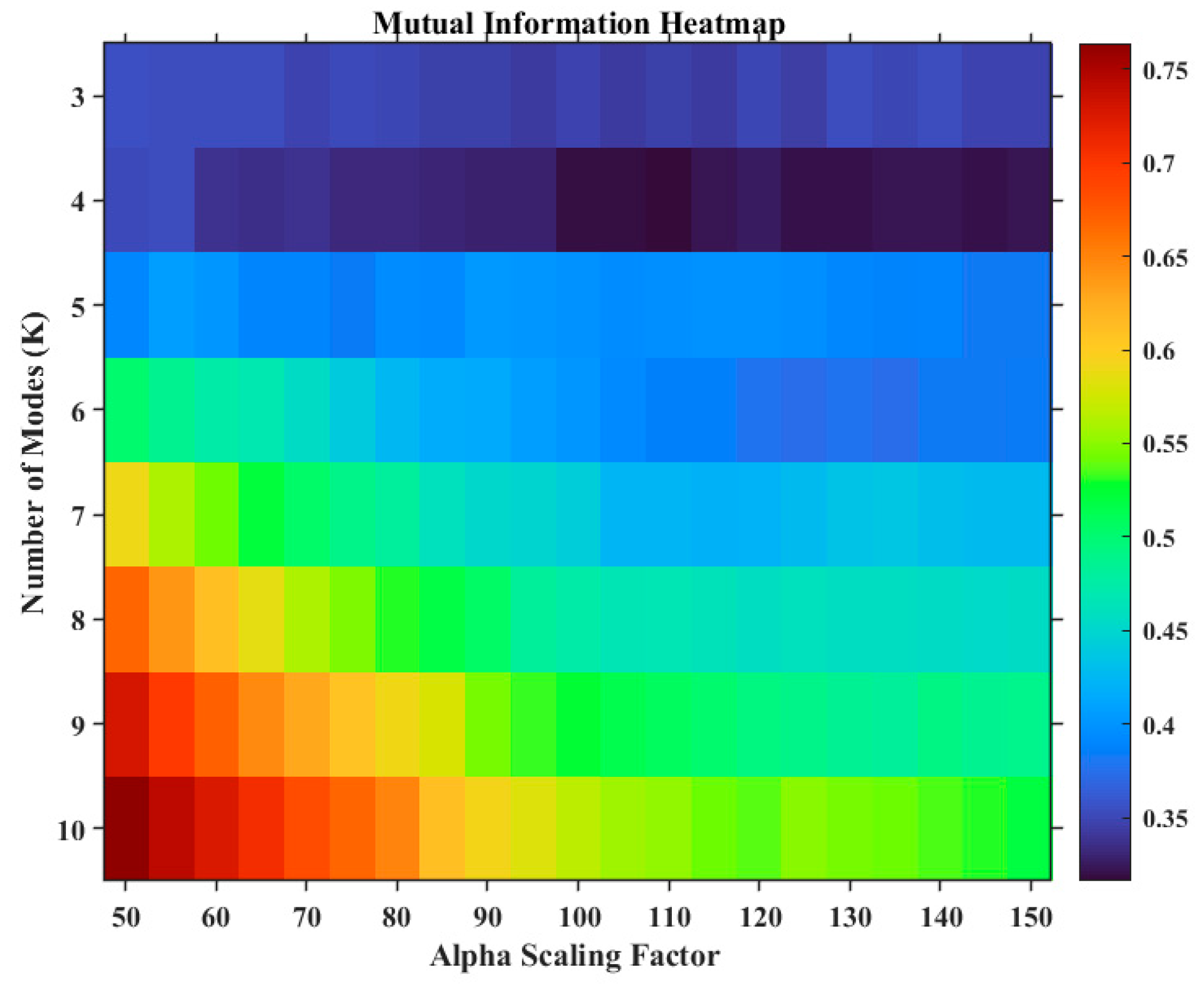
This section describes the methodologies involved in the hybrid prediction model proposed in this paper.

2.1. VMD Algorithm

Variational Mode Decomposition (VMD) is an adaptive signal processing method proposed by Dragomiretskiy et al. [37]. The core idea of VMD is to decompose a given signal into multiple Intrinsic Mode Functions (IMFs) based on specific central frequencies and finite bandwidths. In the context of monitoring the construction of super high-rise buildings, accelerometer data often obscure key features due to noise and complex environmental disturbances. VMD allows the decomposition of acceleration signals into several physically meaningful modal components, each corresponding to different frequency ranges and dynamic characteristics, highlighting the signal’s features to provide a clearer and more accurate input data foundation for subsequent predictions using TCNs [38].
The decomposition process is as follows:
(1)
Utilize the Hilbert transform to obtain the one-sided spectrum of the signal:
δ ( t ) + j π t × v k ( t )
(2)
Convert the spectrum into a baseband by multiplying it with an exponential signal at the estimated center frequency:
δ ( t ) + j π t v k ( t ) e j ω k t
(3)
Estimate the bandwidth by Gaussian smoothing of the demodulated signal, represented as a constrained variational problem in Equation (3):
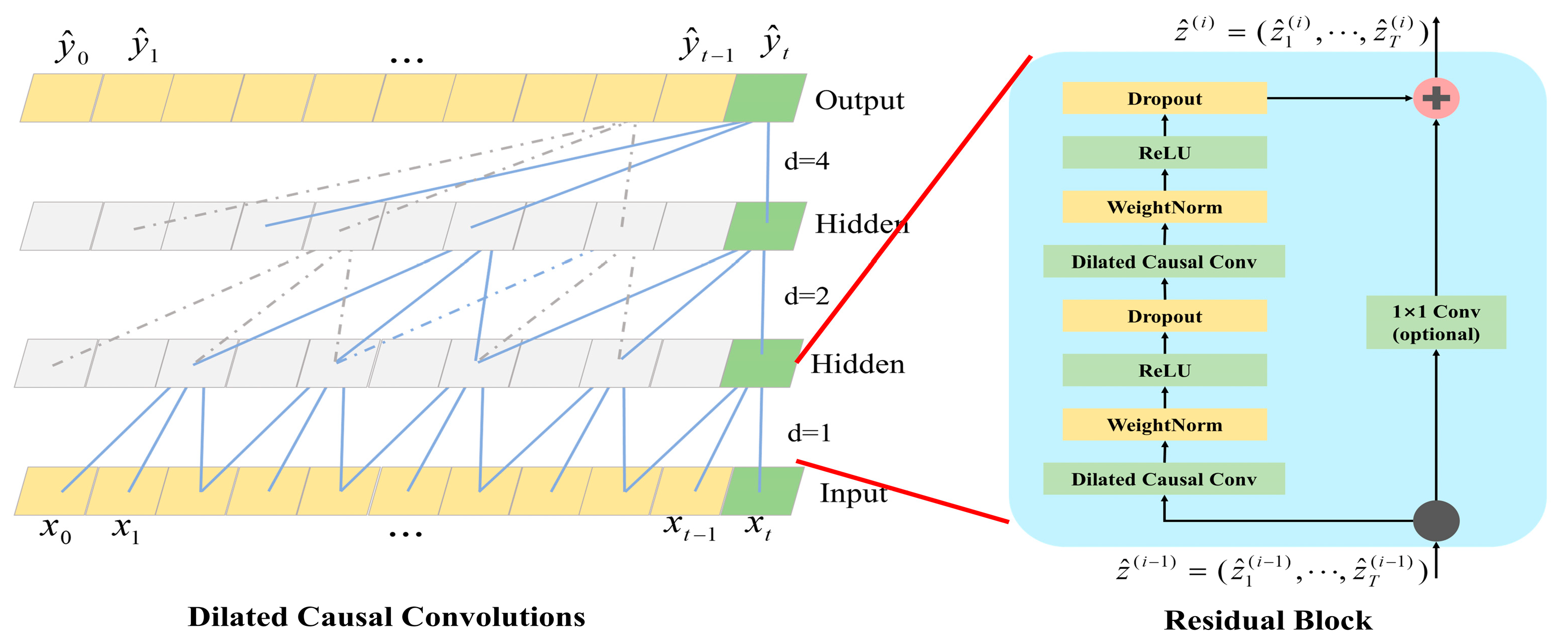
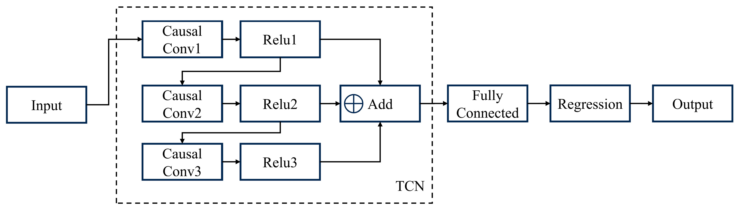
min { v k } , { ω k } k = 1 K t δ ( t ) + j π t × v k ( t ) e j ω k t 2
In Equations (1)–(3), t represents the derivative with respect to time; δ ( t ) + j π t is the Hilbert transform, used for computing the unilateral spectrum; δ ( t ) is the unit pulse signal v k ( t ) denotes the kth mode, and ω k is the central frequency of the kth mode; the constraint is that the sum of all modes should restore the original signal, denoted as k = 1 K v k ( t ) = f ( t ) .
To transform the above constrained variational problem into an unconstrained problem, a Lagrange multiplier λ, and a penalty parameter α are introduced, resulting in an augmented Lagrangian function:
L ( { v k } , { ω k } , λ ) = R + F
R = k = 1 K α t δ ( t ) + j π t v k ( t ) e j ω k t 2
F = f ( t ) k = 1 K v k ( t ) 2 + λ ( t ) , f ( t ) k = 1 K v k ( t )
In the formula, L denotes the augmented Lagrangian function; R and F correspond to the bandwidth penalty term and the signal reconstruction error term, respectively; α represents the balancing parameter; λ ( t ) denotes the Lagrange multiplier; , is the inner product symbol; denotes the convolution operator.
Utilizing the Alternating Direction Method of Multipliers (ADMMs), each mode v k ( t ) and its corresponding central frequency ω k are iteratively updated in the frequency domain to converge to the optimal solution.
v ˜ k n + 1 ( ω ) = f ˜ ( ω ) i k v ˜ i ( ω ) + λ ˜ ( ω ) 2 1 + 2 α ( ω ω k ) 2
ω k n + 1 = 0 ω v ˜ i ( ω ) + 2 d ω 0 v ˜ i ( ω ) + 2 d ω
In the formula, v ˜ k n + 1 ( ω ) represents the update of the kth mode in the frequency domain; f ˜ ( ω ) is the Fourier transform of the original signal; λ ˜ ( ω ) denotes the Fourier transform of the Lagrange multiplier.

2.2. TCN Algorithm

Temporal Convolutional Networks (TCNs) is a deep learning model specifically designed for time series analysis, capable of efficiently capturing long-term dependencies and multi-scale temporal features [39]. Compared to traditional Convolutional Neural Networks [40] (CNNs), Long Short-Term Memory (LSTM) networks, and Gated Recurrent Units [41] (GRUs), the TCN model features a lightweight structure and can flexibly control the receptive field by adjusting the size of the convolutional kernels, making it particularly suitable for time series prediction tasks [42,43]. The model framework is as shown in Figure 1.
The TCN model is applied to monitor the vibrational data for scaffolding safety. The model primarily comprises the following components:
(1)
Causal Convolution
Causal convolution is one of the key components of the TCN, designed to operate on current and past values to estimate current outcomes, while preventing leakage of information from future time steps. However, similar to other neural networks, due to its small kernel size, it struggles to capture long-term dependencies. Causal convolutions require deeper network layers or larger kernel sizes to expand their receptive fields, enabling the capture of dependencies over longer time spans.
(2)
Dilation Convolution
To expand the receptive field without increasing the number of parameters, the TCN model incorporates dilated convolution. Dilated convolution introduces gaps between elements in the convolutional kernel (dilation factor d), thereby enlarging the receptive field while keeping the dimensions of the output feature map constant. By adjusting the value of the dilation factor d (e.g., d = 1, 2, 4, …), the receptive field of the convolutional kernel can be effectively expanded while maintaining the same number of network parameters. This design allows the TCN to efficiently capture long-span temporal features. The mathematical expression is as follows:
F ( s ) = i = 0 k 1 f ( i ) X s d i
In the formula, denotes the convolution result at X s , d represents the dilation factor; f denotes the convolutional kernel; k indicates the size of the convolutional kernel; s d · i represents the index of input at time step s going back by i steps.
(3)
Residual Block
The TCN model employs residual blocks to mitigate issues of gradient vanishing and explosion in deep networks. The core idea of the residual block is to use “skip connections” that add the input directly to the output, thus effectively preserving key input information while enhancing the network’s depth and nonlinear modeling capabilities. Specifically, the structure of the residual block includes two convolutional layers equipped with dilated causal convolution, each layer featuring weight normalization, ReLU activation function, and Dropout regularization. Ultimately, a convolutional layer adjusts the output dimensions to match the input dimensions and implements the residual connection. The formula is as follows:
c = Activation ( x + F ( x ) )
In the formula, x is the input; F ( x ) is the result after convolutional transformation; the Activation function typically used is ReLU (Rectified Linear Unit).

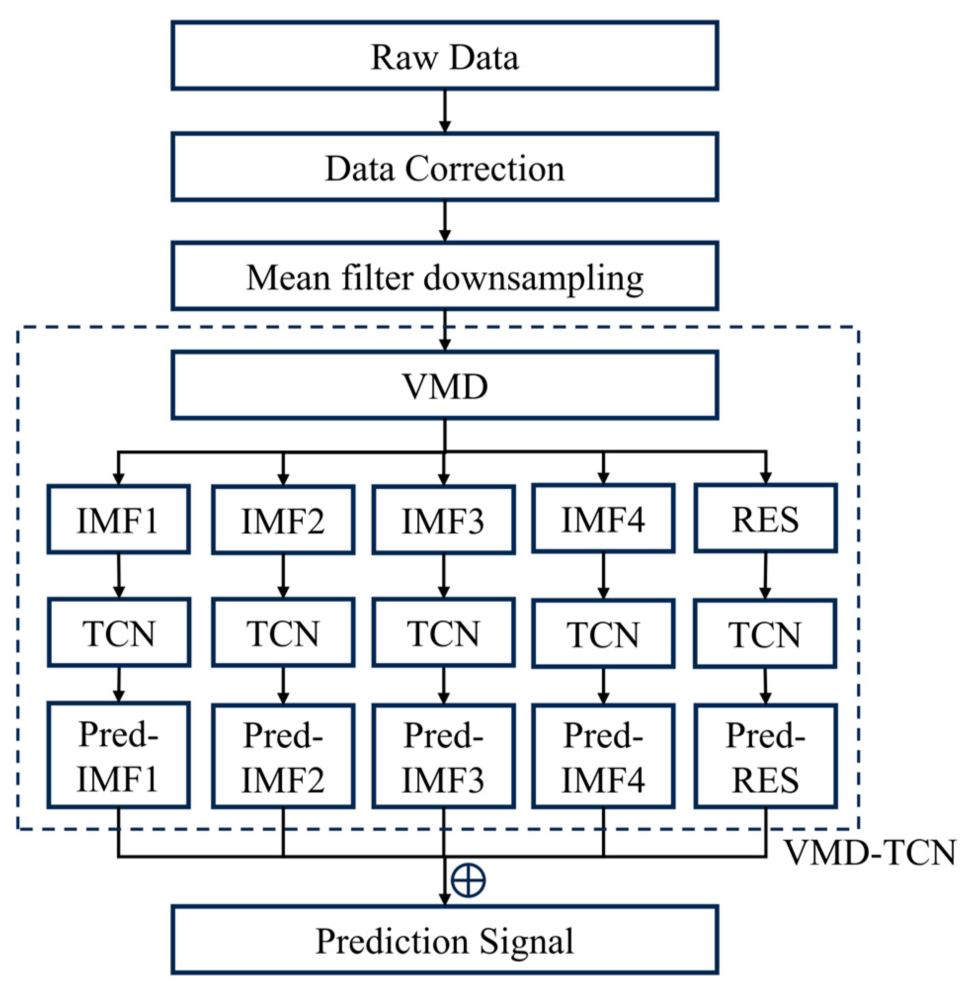
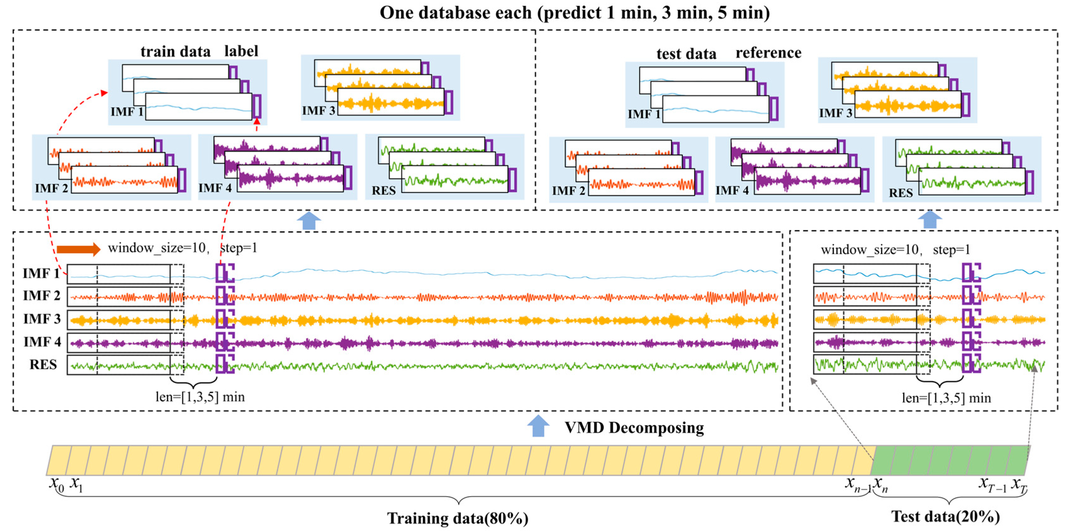
2.3. VMD-TCN Vibration State Prediction Model

This paper presents a hybrid model based on VMD and TCN, designed to achieve high-precision prediction of the vibrational states of construction scaffolding. The VMD-TCN model combines the refined capability of VMD in signal decomposition with the efficiency of TCN in time series modeling to independently predict and capture the dynamic characteristics of multimodal components of vibration signals.
Initially, the VMD is utilized to decompose the corrected scaffolding acceleration vibration data, breaking down the original vibration signal into four IMFs and a residual component. Each IMF corresponds to different frequency ranges, reflecting the signal’s characteristics across various time scales, while the residual component contains details and potential noise not captured by the modal components. Subsequently, for each decomposed IMF and the residual component, independent TCN models are constructed for prediction. Each TCN model employs causal convolution to ensure that the outputs at each time step depend solely on historical inputs, preventing the leakage of future information; dilated convolution is used to expand the receptive field, capturing long-span dependencies without increasing the number of parameters. To further enhance prediction accuracy, the TCN incorporates a residual connection mechanism, using “skip connections” to mitigate the problem of vanishing gradients and enhance the stability of deep networks. Finally, after predicting each IMF and the residual component through separate TCNs, the predicted outcomes of the components are summed to reconstruct the complete vibration signal prediction.
By employing a componentized modeling strategy, the proposed VMD-TCN model is capable of precisely predicting the vibrational state of construction scaffolding, providing a scientific basis for safety warnings during construction and offering significant technical support for the intelligent monitoring and management of super high-rise building construction. The VMD-TCN vibration state prediction model framework is as shown in Figure 2.
To evaluate the precision of the model presented in this paper relative to existing models, the Root Mean Square Error (RMSE), Mean Absolute Error (MAE), and Coefficient of Determination (R2) are utilized to quantify the differences between the model predictions and actual observations.
RMSE = 1 n i = 1 n ( y i y ^ i ) 2
MAE = 1 n i = 1 n | y i y ^ i |
R 2 = 1 ( y i y ^ i ) 2 ( y i y ¯ ) 2
In the formula, y i represents the actual value for the ith instance, y ^ i denotes the predicted value for the ith instance, and n is the number of observation points.

3. Experimental Validation

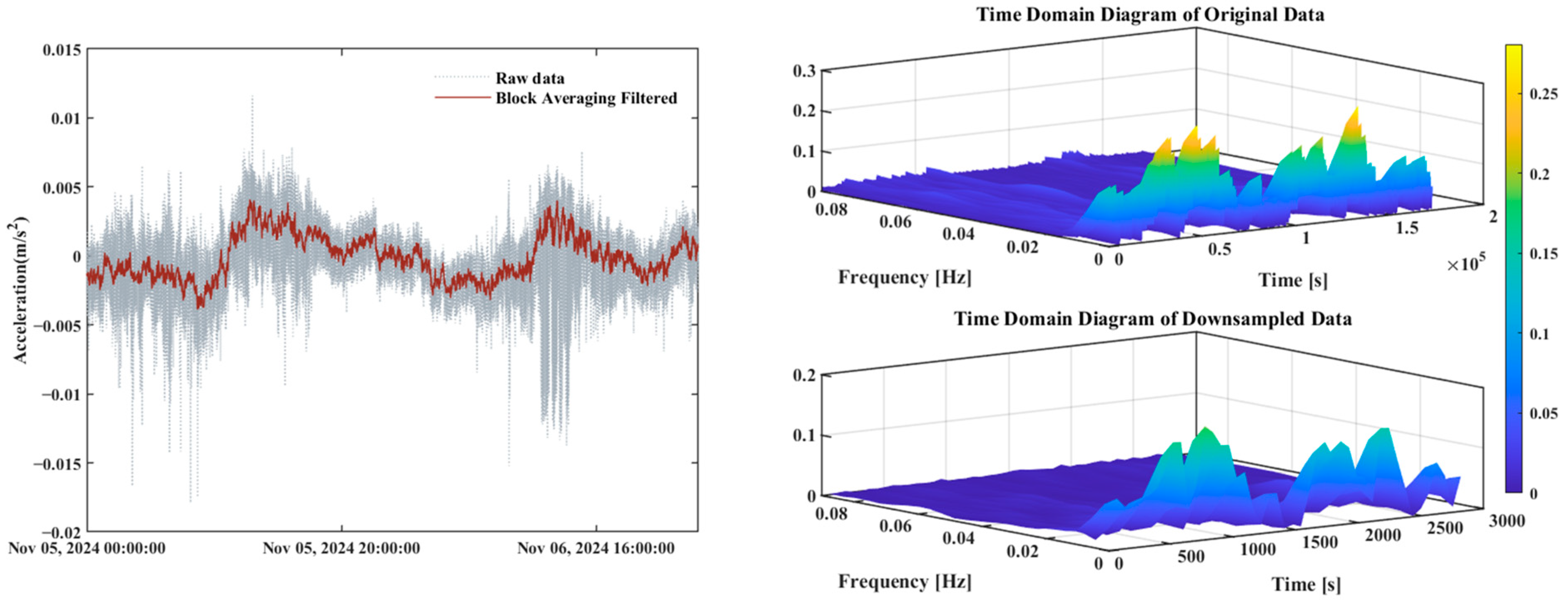
3.1. Collection and Preprocessing of Vibration State Data

The data for this study were sourced from the construction scaffolding health monitoring project at the main office tower of Tianjin Zhonghai Urban Square, which is designed to reach a height of 339.9 m. For this project, low-cost accelerometers were used for real-time dynamic monitoring of the construction scaffolding’s safety to ensure the safety and stability of the climbing scaffold during construction. The accelerometer used in this study is the LSM6DSRTR 3D accelerometer unit, which is installed at the right-angle edges of the four sides of the climbing frame, as shown in Figure 3. The LSM6DSRTR accelerometer utilizes MEMS (Micro-Electro-Mechanical Systems) technology and supports FIFO (First-In-First-Out) data batch processing, which helps reduce system power consumption and enhance data processing efficiency. This makes it particularly suitable for long-term monitoring tasks in construction environments. This paper selects acceleration data from 5 November 2024, 00:00:00 to 7 November 2024, 00:00:00, a total of 48 h, to validate the performance of the proposed vibration state prediction model.
However, due to factors such as uneven installation bases or environmental conditions like wind and rainfall, accelerometers may tilt, causing the gravity acceleration, which should only be present on the Z-axis, to erroneously spread across all three axes. To correct these tilt errors, this paper calculates the device’s attitude angles. Subsequently, using the computed attitude angles, the acceleration data are corrected with rotation matrices to obtain the gravity component corresponding to the Z-axis direction.
To visually observe the vibrations of the scaffolding, this paper subtracts Tianjin’s gravitational acceleration of 9.8011 m/s2 from the Z-axis acceleration to derive the linear acceleration. To eliminate noise from the original vibration data, this paper employs a block averaging filter [44] to downsample the data from a sampling rate of 1 Hz to 1/60 Hz, achieving data noise reduction and volume reduction, thus reducing the computational load for subsequent prediction tasks. As shown in Figure 4, the time-series curve on the left intuitively illustrates the comparison between the raw and filtered data. The gray curve represents the raw acceleration data, which contains significant high-frequency fluctuations, while the red curve denotes the block averaging filtered data. It is evident that the fluctuations in the filtered data are more stable, and the vibration characteristics are more distinct. The time-frequency comparison diagram on the right further validates that the primary features of the signal have been effectively preserved, enabling a more stable learning of vibration patterns and ultimately improving the accuracy and computational efficiency of the predictive model.

3.2. VMD-TCN Vibration State Prediction Model Database Construction

To further explore the intrinsic dynamic characteristics of the acceleration signal, this study employs VMD to decompose vibration state data, extracting modal information of different frequency components. To optimize the key parameter configuration of VMD, Mutual Information (MI) [45] is introduced as an evaluation metric to quantify the independence between different modes. A systematic search is conducted for the number of modes K and the data fidelity balancing parameter α, where the number of modes K is set within the range [3, 10] with a step size of 1, and the balancing parameter α is set within the range [50, 150] with a step size of 5. For each parameter combination, the mean mutual information (MI_avg) of the decomposed modes is calculated, and the optimal mode number and balancing parameter are determined based on the minimum MI_avg value, resulting in K = 4 and α = 110. Other parameters include frequency initialization set to 1, indicating uniform distribution initialization of center frequencies, and a convergence tolerance set to 1 × 10⁻⁷, ensuring sufficient precision during the optimization process. The heatmap of MI_avg is shown in Figure 5.
To verify the effectiveness of VMD, its decomposition results are compared with those obtained using EMD. As shown in Figure 6, EMD suffers from endpoint effects, leading to a certain degree of spectral overlap between different IMFs, whereas VMD effectively reduces mode mixing and enhances the extraction of features in different frequency bands.
As seen in the above figure, the signal after block averaging filtering still contains complex frequency components. Through VMD, feature signals of different bandwidths can be extracted. The frequencies of IMF1 to IMF4 signals increase sequentially, with IMF1 reflecting the long-term trends or slow changes in the scaffolding; IMF2 to IMF4 represent increasing frequency signals in the data.
This study is based on a preprocessed vibration dataset spanning 48 h from 5 November 2024 to 6 November 2024, divided into training and testing sets in an 80% to 20% ratio to ensure effective training and validation of the model. Subsequently, the VMD method is applied to decompose the vibration signals of the training and testing sets, yielding four IMFs and one residual component. Sliding window techniques are then used to segment each modal component, with window lengths set at 10 min and step lengths at 1 min. Through the movement of the sliding windows, training and testing data for each modal component are constructed. The vibration values for the last 1 min, 3 min, and 5 min of each window are used as labels for the training and testing data, for training and validating the deep learning network prediction model. Figure 7 shows the vibration state prediction model database construction process.

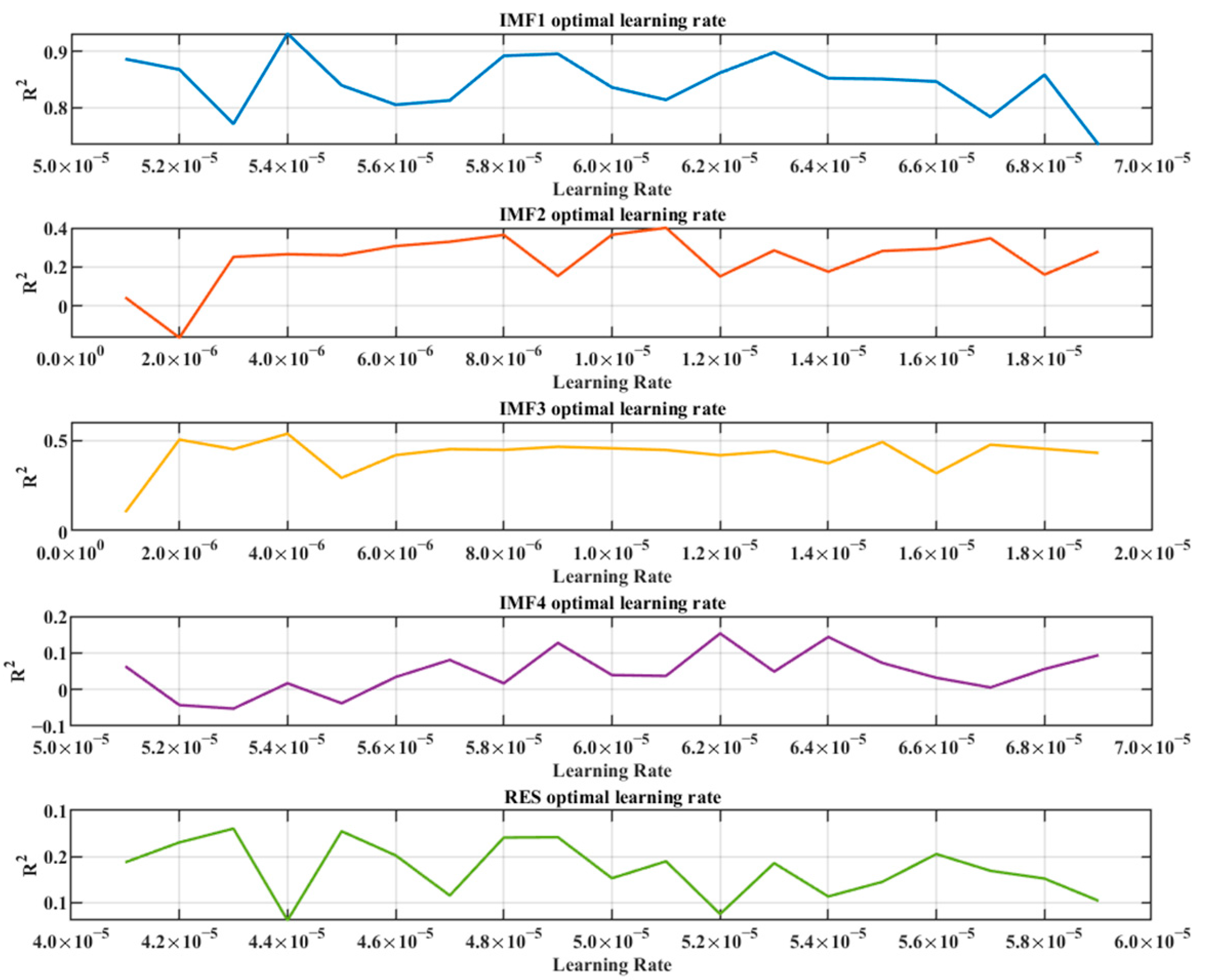
3.3. VMD-TCN Vibration State Prediction Model Training

The TCN model design incorporates multiple layers of one-dimensional convolution structures, causal convolution strategies, and dilated convolution techniques, enabling efficient capture of the time dependencies and multi-scale dynamic characteristics of vibration signals. The TCN is employed to predict vibration sequence data for construction scaffolding. Initially, the input scaffolding vibration data and the modal components data decomposed by VMD are normalized to eliminate scale differences in the data. Subsequently, these are input into multiple one-dimensional convolutional layers using a causal padding strategy to prevent leakage of future data. Each convolutional layer utilizes a kernel size of three units and 32 filters; the first convolutional layer, with a dilation factor of 1, primarily captures short-range dependencies in the sequence; the second layer, with a dilation factor of 2, expands the receptive field to begin capturing longer-range dependencies; the third convolutional layer, with a dilation factor of 4, further increases the receptive field to explore longer-term data dependencies. Each convolutional layer is followed by a ReLU activation function, enhancing the network’s nonlinear processing capability and enabling the model to learn more complex data patterns. Residual connections are then introduced, summing the outputs of the three convolutional layers to optimize the training process and prevent gradient vanishing issues in deep networks. Finally, the data from the residual connection layer are fed into a fully connected layer for regression operations to form the prediction model. Figure 8 shows the VMD-TCN vibration state prediction model data flow diagram.
During the model training phase, the Adam optimizer is utilized, with the maximum number of training epochs set to 60 and the mini-batch size set at 128, to ensure the model is adequately trained within a reasonable computational cost. The learning rate is determined using a grid search method to find the optimal learning rate, which is illustrated in Figure 9.
From the figure, it is evident that different learning rates are employed for different modal components to optimize the final prediction outcomes, with the optimal learning rates for IMF1–4 set, respectively, at 5.40 × 10⁻⁵, 1.10 × 10⁻⁵, 4.00 × 10⁻⁵, 6.20 × 10⁻⁵, and the optimal learning rate for the residual component at 4.30 × 10⁻⁵. Upon completion of training, the test dataset is input into the VMD-TCN model that has been trained, for validation. The results predicted by the model are then subjected to inverse normalization to restore the data to its original scale, facilitating the assessment and analysis of actual effects.

3.4. Vibration State Prediction Model Performance Analysis

Current time series prediction approaches primarily include mathematical model fitting, single network models, and hybrid models. This study employs a sinusoidal fitting model [46], the commonly used time series prediction model GRU network, and the VMD-TCN vibration state prediction model to forecast the time series of the vibrational states of construction scaffolding.

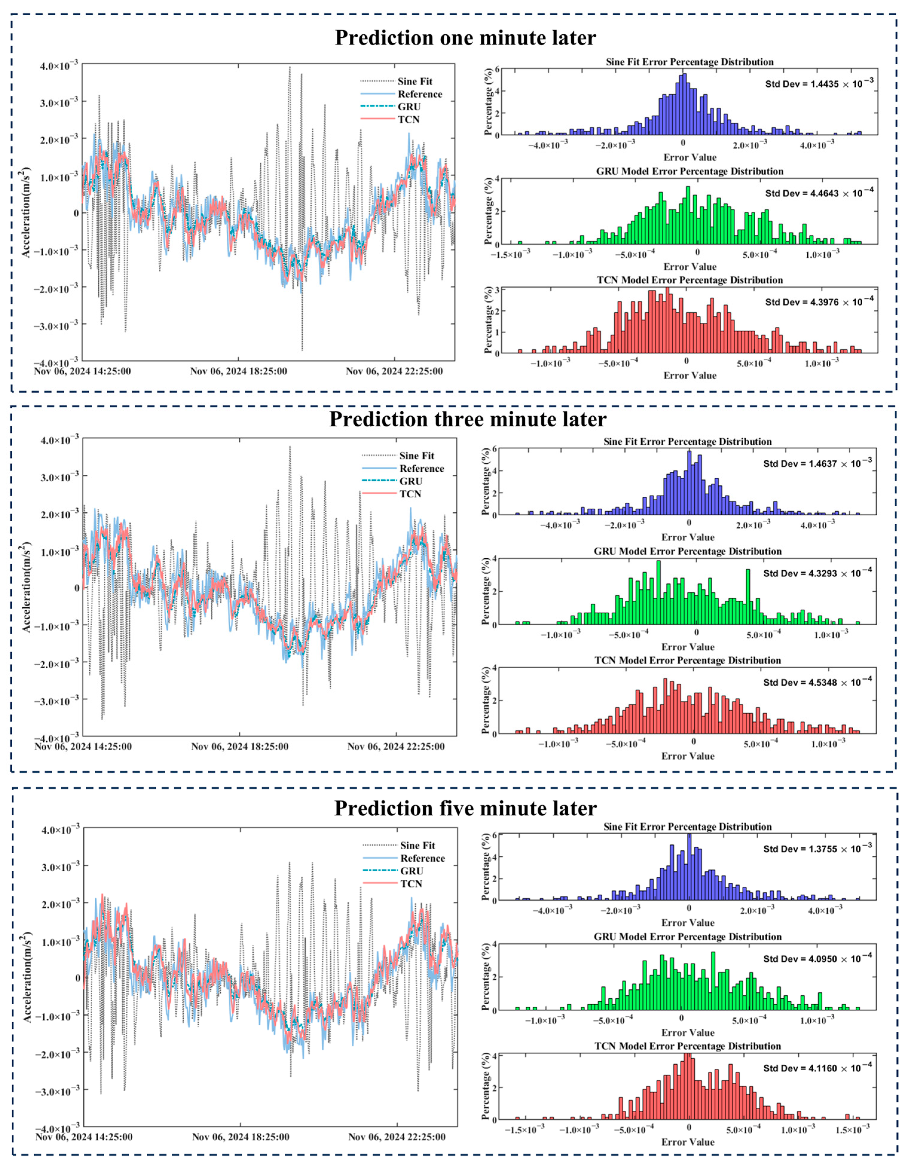
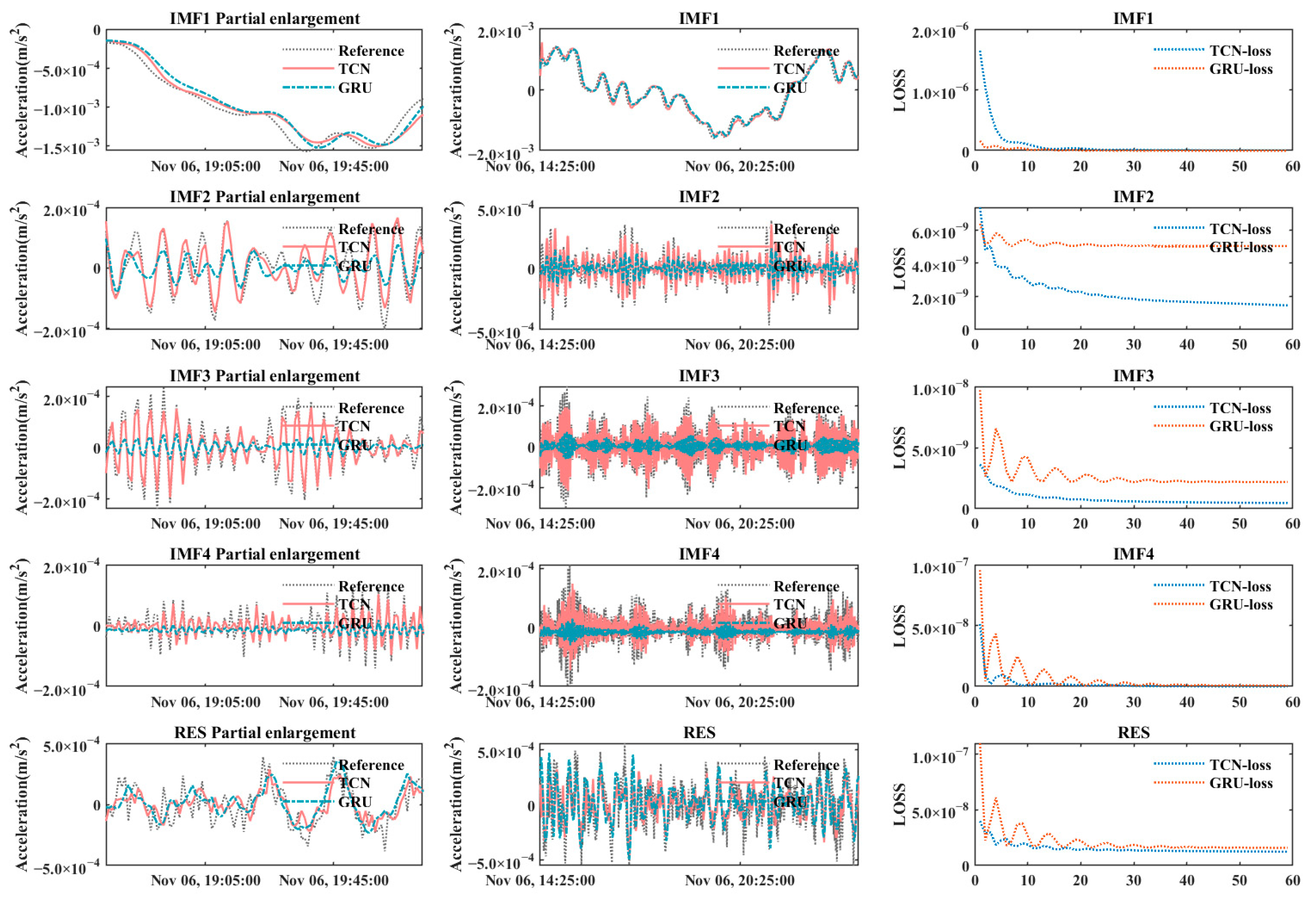
3.4.1. TCNs, GRUs, and Sinusoidal Wave Fitting Vibration State Prediction Model Accuracy Analysis

The sinusoidal wave fitting model excels at capturing the periodic trends of signals by extracting the main frequency components, offering a good fit for vibration-type data; the GRU network, a type of recurrent neural network, resolves issues with long-term memory and gradient problems in RNNs, and is commonly used for modeling nonlinear relationships in time series.
To analyze the performance of the sinusoidal wave fitting model, GRU deep learning network, and TCNs in predicting the vibration states of super high-rise scaffolding, undecomposed one-dimensional vibration data from the scaffolding are input into the sinusoidal wave fitting model, TCN, and GRU network prediction models. Like the deep learning networks, the sinusoidal wave fitting model uses the first ten minutes of vibration data to fit the model, then predicts the vibration values 1 min, 3 min, and 5 min later. The prediction results obtained by the three methods are shown in Figure 10.
The figure indicates that predictions using sinusoidal wave fitting for the 1 min, 3 min, and 5 min acceleration time series are unable to ideally fit the acceleration trends and vibration scenarios. The deviation is primarily distributed between (−0.005, 0.005), which is significantly greater than the prediction deviation of GRU and TCN deep learning networks (−0.002, 0.002). The standard deviation of the sinusoidal wave fitting’s bias is significantly larger than that of the deep learning networks. The prediction capabilities of the TCN and GRU networks are comparable when applied to the raw, undecomposed signals.
To evaluate the predictive performance of each model, Root Mean Square Error (RMSE), Mean Absolute Error (MAE), Coefficient of Determination (R2), and training time are used as metrics to measure the prediction accuracy and computational efficiency of each model. The accuracy comparison of each model is shown in the table below:
From Table 1, it can be observed that in terms of prediction accuracy, the RMSE and MAE values of both TCNs and GRUs are significantly lower than those of the SIN model. The RMSE of the TCN network increases slightly from 4.40 × 10⁻⁴ at 1 min to 5.19 × 10⁻⁴ at 3 min and 5.70 × 10⁻⁴ at 5 min, while the corresponding MAE values are 3.53 × 10⁻⁴, 4.14 × 10⁻⁴, and 4.43 × 10⁻⁴. The RMSE exhibits a slight increase with the extension of the prediction horizon, with growth rates of approximately 17.95% and 9.83%, while the increase in MAE is about 17.28% and 7.00%. In comparison, the RMSE values of the GRU model are 4.46 × 10⁻⁴, 5.17 × 10⁻⁴, and 5.56 × 10⁻⁴, while the MAE values are 3.57 × 10⁻⁴, 4.13 × 10⁻⁴, and 4.36 × 10⁻⁴, showing a prediction performance close to that of TCNs. On the other hand, the SIN model exhibits significantly higher prediction errors than both TCNs and GRU, with RMSE values ranging between 1.40 × 10⁻³ and 1.46 × 10⁻³, and MAE values between 9.97 × 10⁻⁴ and 1.03 × 10⁻³, which fail to meet the required prediction accuracy. Regarding the coefficient of determination (R2), both TCNs and GRUs exhibit values below 80%, indicating that neither model achieves highly accurate predictions. The R2 values for TCNs at the 1 min, 3 min, and 5 min prediction horizons are 76.55%, 67.21%, and 60.39%, respectively, with only minor differences compared to GRUs. The R2 of SIN is negative across all time steps, indicating complete failure to fit the data, with a prediction effect far inferior to TCNs and GRU. In terms of computational efficiency, TCN demonstrates exceptionally high efficiency, with a training time consistently below 1.2 s, which is significantly lower than the GRU model, which requires over 9 s for training. Meanwhile, the fitting time for the SIN model is approximately 5.5 s. This indicates that compared to traditional mathematical fitting model prediction methods, using deep learning algorithms provides higher accuracy in predicting the vibration states of scaffolding.

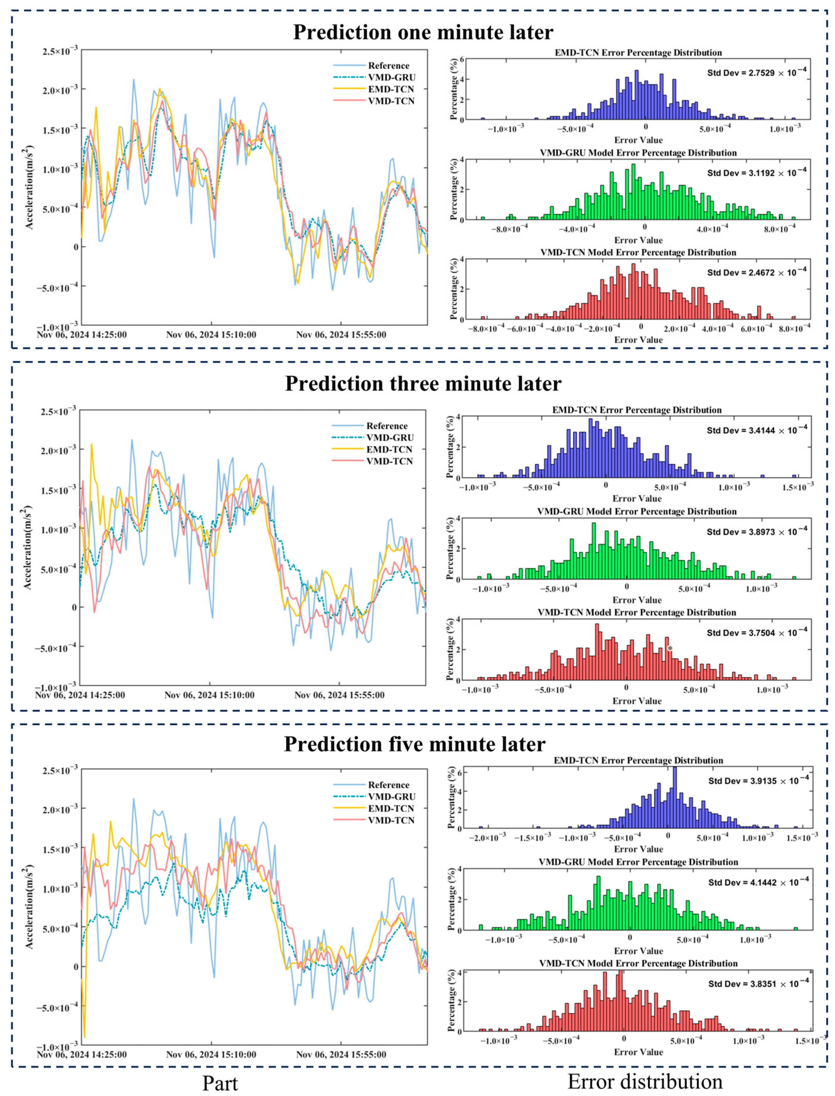
3.4.2. VMD-TCN and VMD-GRU Vibration State Prediction Model Accuracy Analysis

Direct predictions using undecomposed signals struggle to capture the nonlinear and complex variations in signals, resulting in TCN and GRU models not effectively predicting the scaffolding vibration, with both models’ R2 values not exceeding 80%. To address this, the original signals are decomposed into multiple IMFs using VMD, allowing for separate predictions of different frequency and time-scale features. The results and the training loss curve are shown in Figure 11.
As shown in Figure 11 and Table 2, TCNs and GRUs have comparable performance in predicting low-frequency signals as evidenced by IMF1. For signals with high-frequency components, as shown in IMF2–4, the GRU network struggles to precisely predict high-frequency vibrations and can only approximate the overall trend. The TCN model, however, accurately predicts both low-frequency trend signals and high-frequency vibrations. Compared to traditional GRU time series networks, the TCN network shows a significant improvement in each component’s prediction accuracy by 0.09%, 107.06%, 185.74%, 190.08%, and 72.21%, respectively.
This study integrates VMD and EMD methods, summing the predicted components and residuals from TCN and GRU networks to obtain the predicted signals at different time steps, as shown in Figure 12. The comparison of signal metrics is presented in the Table 3.
From the above figure, it can be observed that the TCN network outperforms the GRU network in predicting vibration signals at different time steps (1 min, 3 min, and 5 min intervals). The VMD-TCN model effectively captures the short-term details of vibration signals, whereas the VMD-GRU model exhibits higher errors in regions with significant local fluctuations, leading to noticeable oscillations in the prediction curve and difficulty in accurately fitting short-term signal variations. The EMD-TCN model demonstrates local fitting performance that falls between VMD-TCN and VMD-GRU. The standard deviation of errors indicates that VMD-TCN achieves the lowest prediction errors across all time steps. Compared to VMD-GRU, the standard deviation of VMD-TCN prediction errors is reduced by 48.72%, 41.38%, and 36.65% for 1 min, 3 min, and 5 min predictions, respectively.
To further verify the stability of model prediction errors, this study calculates the prediction error distribution intervals for different models at a 95% confidence level, as shown in Table 3. It can be observed that VMD-TCN has the narrowest confidence interval, indicating the best prediction stability and the lowest error fluctuation. In contrast, VMD-GRU exhibits a wider error distribution interval, leading to less stable predictions, especially for long-term forecasts (3 min and 5 min), where error fluctuations are more pronounced.
From Table 4, it can be observed that after applying EMD and VMD, the prediction accuracy of the original TCN and GRU models has significantly improved. Among all models, VMD-TCN demonstrates the best overall performance across various evaluation metrics, further validating the effectiveness of VMD in signal decomposition. Compared to the other models, VMD-TCN achieves the best balance between prediction accuracy and computational efficiency, making it the optimal choice for vibration state prediction.
In terms of Root Mean Square Error (RMSE) and Mean Absolute Error (MAE), VMD-TCN outperforms all other models across all time steps. The RMSE values for 1 min, 3 min, and 5 min predictions are 2.47 × 10⁻⁴, 2.95 × 10⁻⁴, and 3.72 × 10⁻⁴, respectively, representing reductions of 21.1%, 21.9%, and 17.3% compared to VMD-GRU, and reductions of 10.2%, 13.5%, and 1.8% compared to EMD-TCN. While EMD-TCN achieves lower RMSE than VMD-GRU, it is still higher than VMD-TCN, indicating that EMD improves prediction accuracy but is slightly inferior to VMD in terms of decomposition effectiveness. Regarding MAE, VMD-TCN maintains the best performance, reducing MAE by 21.3%, 21.9%, and 18.3% compared to VMD-GRU for the 1 min, 3 min, and 5 min predictions, respectively, and reducing it by 7.1%, 10.9%, and 0% (with identical values at 5 min) compared to EMD-TCN.
In terms of signal fitting capability, EMD-TCN demonstrates better R2 values than VMD-GRU, achieving 90.84%, 85.87%, and 82.51% for the 1 min, 3 min, and 5 min predictions, respectively, representing improvements of 3.1%, 3.9%, and 9.5% over VMD-GRU. VMD-TCN achieves the highest R2 values across all time steps, reaching 92.61%, 89.41%, and 83.11%. Compared to EMD-TCN, VMD-TCN further improves R2 by 1.9%, 4.1%, and 0.7% for 1 min, 3 min, and 5 min predictions, respectively, demonstrating that VMD is superior in extracting both low-frequency trends and high-frequency features. This highlights the advantage of VMD-TCN in modeling the complex characteristics of vibration signals.
Regarding model training time, VMD-TCN exhibits the shortest training duration, with prediction times of 5.72 s, 5.58 s, and 5.67 s for the 1 min, 3 min, and 5 min forecasts, respectively. This represents reductions of 90.3%, 88.9%, and 88.5% compared to VMD-GRU, and reductions of 5.6%, 23.7%, and 28.6% compared to EMD-TCN. These results indicate that VMD-TCN achieves the best balance between prediction accuracy and computational efficiency, making it well-suited for engineering applications with high real-time requirements.

3.4.3. Influence of Different Training Window Lengths on Prediction Accuracy

The previous sections conducted a comprehensive analysis of the performance of different prediction models. In this, the influence of different training window lengths on prediction accuracy is further investigated based on the VMD-TCN model. Four different sliding window lengths, namely 5 min, 10 min, 15 min, and 20 min, were selected to construct a vibration signal prediction dataset, and their performance was evaluated using a 1 min prediction time step. Table 5 presents the RMSE, MAE, R2, and training time under different training window lengths.
Experimental results indicate that when the sliding window length is set to 10 min, the prediction accuracy reaches its highest level, with the lowest RMSE of 2.47 × 10⁻⁴, the lowest MAE of 1.96 × 10⁻⁴, and the highest R2 of 92.61%, demonstrating that the 10 min training window optimally captures the dynamic characteristics of the vibration signal. Additionally, the training time results show that the length of training data has a minimal impact on computational efficiency. The computation time for the 10 min window (5.72 s) exhibits no significant difference compared to the other window lengths (5 min, 15 min, and 20 min), confirming that increasing the training window length does not substantially increase computational cost.

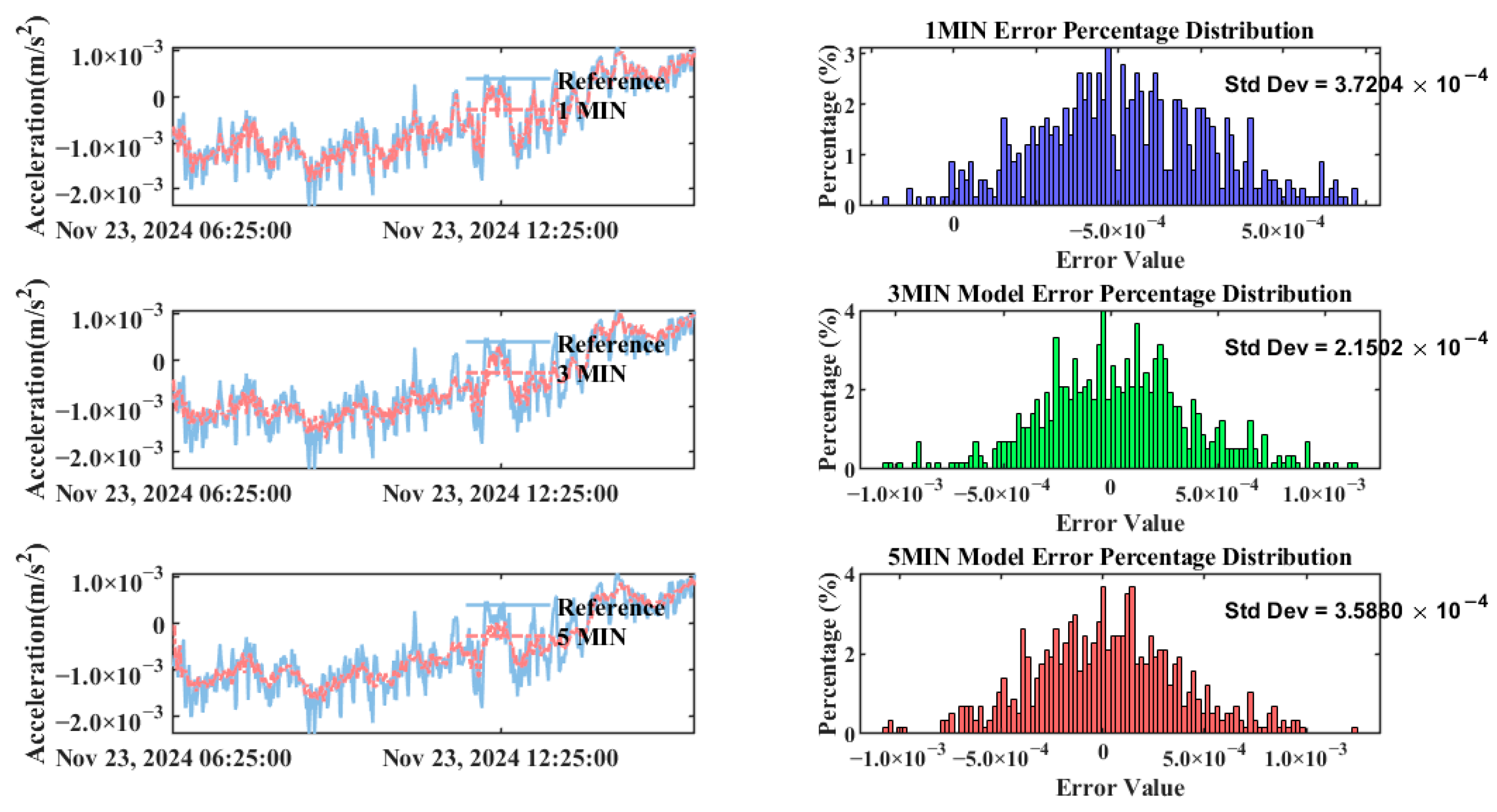
3.4.4. Verification of Model Data Applicability

To validate the applicability of the VMD-TCN model across different datasets, this study selected data from another accelerometer (21 November 2024, 16:00:00 to 23 November 2024, 15:59:59, totaling 48 h) for prediction. The prediction accuracy was compared with the results of the previously used dataset to evaluate the model’s generalization ability in different data environments. This ensures that the model is suitable for climbing frame vibration monitoring tasks under varying sensor and data conditions. The prediction results and errors are presented in Table 6 and Figure 13.
Experimental results demonstrate that VMD-TCN maintains high prediction accuracy across different datasets, exhibiting strong generalizability in varying data environments. The error distribution follows a normal distribution, indicating stable model errors and adaptability to different data characteristics. Additionally, the computational efficiency remains consistent, confirming that the model can achieve stable and reliable vibration state predictions for climbing frames.

4. Conclusions

This paper addresses the demand for accurate vibration state prediction during the construction of super high-rise buildings. Taking the climbing scaffolding of Tianjin Zhonghai City Square as a case study, a vibration prediction model combining VMD and TCNs was proposed. The model was validated using 48 h of scaffolding vibration data, evaluating predictions at 1 min, 3 min, and 5 min intervals. The key conclusions are as follows:
(1)
VMD significantly enhances multi-frequency feature extraction capability. Compared to raw vibration signals, VMD modal signals (IMF1~IMF4) better represent low-frequency trends and high-frequency details, providing richer and more accurate feature inputs for deep learning models. Experimental results indicate that VMD effectively reduces mode mixing compared with EMD. Following VMD, the prediction accuracies of TCN and GRU networks improved substantially. Compared to predictions from unprocessed signals, the VMD-TCN model reduced RMSE by 43.9%, 43.2%, and 34.7% at 1 min, 3 min, and 5 min intervals, respectively, while improving R2 by 21.0%, 33.0%, and 37.6%. Similarly, the VMD-GRU model showed RMSE reductions of 29.9%, 26.9%, and 19.1%, with corresponding R2 improvements of 16.2%, 15.14%, and 20.9%.
(2)
The TCN model demonstrates superior predictive accuracy and computational efficiency. Compared to the GRU model, the TCN is particularly adept at handling high-frequency features. Specifically, for high-frequency modal components (IMF2, IMF3, and IMF4) obtained through VMD, the TCN achieved R2 values of 81.50%, 86.35%, and 63.18%, respectively—significantly higher than GRU’s corresponding values of 39.36%, 30.22%, and 21.78%. Overall, VMD-TCN achieved RMSE values of 2.47 × 10⁻⁴, 2.95 × 10⁻⁴, and 3.72 × 10⁻⁴ at 1 min, 3 min, and 5 min predictions, representing decreases of 21.1%, 21.9%, and 17.3% compared to VMD-GRU, respectively. Additionally, the training time for VMD-TCN was consistently between 5.58 and 5.72 s, significantly faster than VMD-GRU’s 49.49 to 58.88 s, demonstrating approximately 88–91% improvement in computational efficiency. Therefore, the TCN is more suitable for real-time applications requiring high responsiveness in practical engineering scenarios.
(3)
The VMD-TCN model exhibits strong generalization capability. Experimental validation across two independent datasets collected from different sensor locations and acquisition periods demonstrated stable and consistently high prediction accuracy. The new dataset yielded R2 values of 92.47%, 86.86%, and 81.09% for predictions at 1 min, 3 min, and 5 min intervals, respectively, closely matching the original dataset results (92.61%, 89.41%, 83.11%). Furthermore, prediction error distributions were normally distributed with low standard deviations (4.58 × 10⁻⁴, 4.01 × 10⁻⁴, and 3.47 × 10⁻⁴), and computational efficiency remained stable at around 5 s. These findings suggest the VMD-TCN model’s robustness and reliability, making it suitable for broader applications in vibration prediction tasks for super high-rise building construction.
Despite the demonstrated high predictive accuracy and excellent computational efficiency of the VMD-TCN model, several areas remain for further research:
(1)
Diversity in environmental conditions and scaffolding types. This study primarily evaluated aluminum climbing scaffolds in Tianjin. Applying the model under varied climatic conditions, materials (e.g., steel or composites), and different scaffolding types requires further investigation. Future research should gather vibration data from various construction sites to thoroughly assess the model’s adaptability and generalization performance in complex scenarios.
(2)
Currently, MEMS accelerometers were installed empirically, with only one sensor placed on each face of the scaffold. Systematic studies on the optimal number, placement, and spatial distribution of MEMS accelerometers are lacking. Identifying an optimal sensor deployment strategy will ensure comprehensive and accurate structural vibration monitoring.
(3)
Future studies could integrate multi-source heterogeneous data, such as wind speed, temperature, load conditions, and construction progress, with vibration signals. Employing multimodal deep learning models could enhance generalization and predictive accuracy in complex construction environments. Combining threshold-based analysis with trend analysis in a hybrid early-warning framework may further facilitate real-time risk identification and proactive construction safety management.
(4)
Determining acceptable vibration thresholds for scaffolding safety. Although the proposed VMD-TCN model significantly reduces prediction errors, practical safety management demands clearly defined vibration safety thresholds. Establishing universally applicable thresholds is challenging, as acceptable vibration levels vary greatly with scaffolding materials, structural design, load conditions, and environmental influences (e.g., wind and seismic forces). Future studies should leverage existing Structural Health Monitoring (SHM) standards and practical engineering insights to define clear vibration safety limits. Developing these thresholds will clarify how prediction accuracy translates into tangible safety improvements, enabling effective risk identification and proactive intervention.

Author Contributions

Conceptualization, P.Z. and J.W.; methodology, P.Z.; software, P.Z. and G.L.; validation, P.Z., G.L. and P.W.; formal analysis, J.W. and P.Z.; investigation, J.W.; resources, J.W.; data curation, P.Z. and G.L.; writing—original draft preparation, P.Z.; writing—review and editing, G.L.; visualization, P.Z.; supervision, G.L.; project administration, J.W. and G.L.; funding acquisition, J.W. and G.L. All authors have read and agreed to the published version of the manuscript.

Funding

This work was supported by the National Natural Science Foundation of China (42404035; 42274029); R&D Program of Beijing Municipal Education Commission (KM202410016007).

Data Availability Statement

The original contributions presented in this study are included in the article. Further inquiries can be directed to the corresponding author(s).

Conflicts of Interest

The authors declare no conflicts of interest.

References

  1. Gong, J.; Fang, T.; Zuo, J. A Review of Key Technologies Development of Super High-Rise Building Construction in China. Adv. Civ. Eng. 2022, 2022, 5438917. [Google Scholar] [CrossRef]
  2. Chen, X.; Li, S.; Yu, Z.; Xu, J.; Wang, L.; Pei, Y.; Zhang, W.; Jing, Z.; Min, L.; Wang, Y. Application of Key Technologies for Multi-Terminal Change of Frame-Double Core Tube Super High-Rise Building. IOP Conf. Ser. Earth Environ. Sci. 2021, 692, 22090. [Google Scholar] [CrossRef]
  3. Nguyen, V.T.; Nguyen, K.A.; Nguyen, V.L. An improvement of a hydraulic self-climbing formwork. Arch. Mech. Eng. 2019, 66, 495–507. [Google Scholar] [CrossRef]
  4. Zhou, H.F.; Ni, Y.Q.; Ko, J.M. A data processing and analysis system for the instrumented suspension Jiangyin Bridge. In Proceedings of the World Forum on Smart Materials and Smart Structures Technology, Nanjing, China, 22–27 May 2008; CRC Press: Boca Raton, FL, USA, 2008; p. 242. [Google Scholar]
  5. Housner, G.W. Behavior of structures during earthquakes. J. Eng. Mech. Div. 1959, 85, 109–129. [Google Scholar] [CrossRef]
  6. Cochran, E.; Lawrence, J.; Christensen, C.; Chung, A. A novel strong-motion seismic network for community participation in earthquake monitoring. IEEE Instrum. Meas. Mag. 2009, 12, 8–15. [Google Scholar] [CrossRef]
  7. Clayton, R.; Heaton, T.; Chandy, M.; Krause, A.; Kohler, M.; Bunn, J.; Guy, R.; Olson, M.; Faulkner, M.; Cheng, M. Community seismic network. Ann. Geophys. 2011, 54, 738–747. [Google Scholar]
  8. Ozer, E.; Feng, M.Q.; Feng, D. Citizen sensors for SHM: Towards a crowdsourcing platform. Sensors 2015, 15, 14591–14614. [Google Scholar] [CrossRef]
  9. Liang, Q.; Tani, A.; Yamabe, Y. Fundamental tests on a structural health monitoring system for building structures using a single-board microcontroller. J. Asian Archit. Build. 2015, 14, 663–670. [Google Scholar] [CrossRef]
  10. Cao, R.; El-Tawil, S.; Agrawal, A.K. Miami pedestrian bridge collapse: Computational forensic analysis. J. Bridge Eng. 2020, 25, 4019134. [Google Scholar] [CrossRef]
  11. Savin S, Y. Influence of shear deformations on the buckling of reinforced concrete elements. In Proceedings of the Innovations and Technologies in Construction: Selected Papers of BUILDINTECH BIT 2021, Belgorod, Russia, 9–10 March 2021; Springer International Publishing: Berlin/Heidelberg, Germany, 2021; pp. 195–200. [Google Scholar]
  12. Lamonaca, F.; Olivito, R.S.; Porzio, S.; Cami, D.L.; Scuro, C. Structural health monitoring system for masonry historical construction. In Proceedings of the 2018 Metrology for Archaeology and Cultural Heritage (MetroArchaeo), Cassino, Italy, 22–24 October 2018; IEEE: Piscataway, NJ, USA, 2018; pp. 330–335. [Google Scholar]
  13. Uva, G.; Sangiorgio, V.; Ruggieri, S.; Fatiguso, F. Structural vulnerability assessment of masonry churches supported by user-reported data and modern Internet of Things (IoT). Measurement 2019, 131, 183–192. [Google Scholar] [CrossRef]
  14. Law, S.; Lin, J. Unit impulse response estimation for structural damage detection under planar multiple excitations. J. Appl. Mech. 2014, 81, 21015. [Google Scholar] [CrossRef]
  15. Lin, J.F.; Xu, Y.L. Two-stage covariance-based multisensing damage detection method. J. Eng. Mech. 2017, 143, B4016003. [Google Scholar] [CrossRef]
  16. Xu, Y.L.; Lin, J.F.; Zhan, S.; Wang, F.Y. Multistage damage detection of a transmission tower: Numerical investigation and experimental validation. Struct. Control Health Monit. 2019, 26, e2366. [Google Scholar] [CrossRef]
  17. Wang, H.; Barone, G.; Smith, A. A novel multi-level data fusion and anomaly detection approach for infrastructure damage identification and localisation. Eng. Struct. 2023, 292, 116473. [Google Scholar] [CrossRef]
  18. Rocha Ribeiro, R.; de Almeida Sobral, R.; Cavalcante, I.B.; Conte Mendes Veloso, L.A.; de Melo Lameiras, R. A Low—Cost Wireless Multinode Vibration Monitoring System for Civil Structures. Struct. Control Health Monit. 2023, 2023, 5240059. [Google Scholar] [CrossRef]
  19. Komarizadehasl, S.; Komary, M.; Alahmad, A.; Lozano-Galant, J.A.; Ramos, G.; Turmo, J. A novel wireless low-cost inclinometer made from combining the measurements of multiple MEMS gyroscopes and accelerometers. Sensors 2022, 22, 5605. [Google Scholar] [CrossRef]
  20. Pierleoni, P.; Marzorati, S.; Ladina, C.; Raggiunto, S.; Belli, A.; Palma, L.; Cattaneo, M.; Valenti, S. Performance evaluation of a low-cost sensing unit for seismic applications: Field testing during seismic events of 2016–2017 in Central Italy. IEEE Sens. J. 2018, 18, 6644–6659. [Google Scholar] [CrossRef]
  21. Ragam, P.; Devidas Sahebraoji, N. Application of MEMS-based accelerometer wireless sensor systems for monitoring of blast-induced ground vibration and structural health: A review. IET Wirel. Sens. Syst. 2019, 9, 103–109. [Google Scholar] [CrossRef]
  22. Sabato, A.; Niezrecki, C.; Fortino, G. Wireless MEMS-based accelerometer sensor boards for structural vibration monitoring: A review. IEEE Sens. J. 2016, 17, 226–235. [Google Scholar] [CrossRef]
  23. Meng, Q.; Zhu, S. Developing iot sensing system for construction-induced vibration monitoring and impact assessment. Sensors 2020, 20, 6120. [Google Scholar] [CrossRef]
  24. Ding, L.Y.; Zhou, C.; Deng, Q.X.; Luo, H.B.; Ye, X.W.; Ni, Y.Q.; Guo, P. Real-time safety early warning system for cross passage construction in Yangtze Riverbed Metro Tunnel based on the internet of things. Automat. Constr. 2013, 36, 25–37. [Google Scholar] [CrossRef]
  25. Rasul, M.; Hosoda, A. Application of artificial neural network in predicting maximum thermal crack width of RC abutments using actual construction data. In Proceedings of the fib Symp, Krakow, Poland, 27–29 May 2019; pp. 1339–1346. [Google Scholar]
  26. Zhong, Z.; Gao, Q.; Zhang, F. Research on classification method of abnormal vibration of pipeline based on SVM. In Proceedings of the Eighth Symposium on Novel Photoelectronic Detection Technology and Applications, Kunming, China, 9–11 November 2022; SPIE: Bellingham, WA, USA, 2022; Volume 12169, pp. 1184–1195. [Google Scholar]
  27. Mistikoglu, G.; Gerek, I.H.; Erdis, E.; Usmen, P.M.; Cakan, H.; Kazan, E.E. Decision tree analysis of construction fall accidents involving roofers. Expert Syst. Appl. 2015, 42, 2256–2263. [Google Scholar] [CrossRef]
  28. Feng, K.; González, A.; Casero, M. A kNN algorithm for locating and quantifying stiffness loss in a bridge from the forced vibration due to a truck crossing at low speed. Mech. Syst. Signal Process. 2021, 154, 107599. [Google Scholar] [CrossRef]
  29. Jiang, L.; Zhao, T.; Feng, C.; Zhang, W. Improvement of random forest by multiple imputation applied to tower crane accident prediction with missing data. Eng. Constr. Archit. Manag. 2023, 30, 1222–1242. [Google Scholar] [CrossRef]
  30. Pan, X.; Zhao, T.; Li, X.; Zuo, Z.; Zong, G.; Zhang, L. Automatic identification of the working state of high-rise building machine based on machine learning. Appl. Sci. 2023, 13, 11411. [Google Scholar] [CrossRef]
  31. Zhou, Q.; Li, Q.; Han, X.; Lu, B.; Wan, J.; Xu, K. Improvement of GPS displacement measurement accuracy for high-rise buildings by machine learning. J. Build. Eng. 2023, 78, 107581. [Google Scholar] [CrossRef]
  32. Slaton, T.; Hernandez, C.; Akhavian, R. Construction activity recognition with convolutional recurrent networks. Automat. Constr. 2020, 113, 103138. [Google Scholar] [CrossRef]
  33. Gao, X.; Shi, M.; Song, X.; Zhang, C.; Zhang, H. Recurrent neural networks for real-time prediction of TBM operating parameters. Automat. Constr. 2019, 98, 225–235. [Google Scholar] [CrossRef]
  34. Sun, M.; Li, Q.; Li, Y. Investigation of time-varying natural frequencies of high-rise buildings under harsh excitations using a high-resolution combined scheme. J. Build. Eng. 2022, 57, 104859. [Google Scholar] [CrossRef]
  35. Manikumar, R.; Singampalli, R.S. Application of EMD based statistical parameters for the prediction of fault severity in a spur gear through vibration signals. Adv. Mater. Process. Technol. 2022, 8, 2152–2170. [Google Scholar] [CrossRef]
  36. Fan, J.; Zhang, K.; Huang, Y.; Zhu, Y.; Chen, B. Parallel spatio-temporal attention-based TCN for multivariate time series prediction. Neural Comput. Appl. 2023, 35, 13109–13118. [Google Scholar] [CrossRef]
  37. Dragomiretskiy, K.; Zosso, D. Variational mode decomposition. IEEE Trans. Signal Process. 2013, 62, 531–544. [Google Scholar] [CrossRef]
  38. Xin, J.; Mo, X.; Jiang, Y.; Tang, Q.; Zhang, H.; Zhou, J. Recovery Method of Continuous Missing Data in the Bridge Monitoring System Using SVMD-Assisted TCN–MHA–BiGRU. Struct. Control. Health Monit. 2025, 2025, 8833186. [Google Scholar] [CrossRef]
  39. Bai, S.; Kolter, J.Z.; Koltun, V. An empirical evaluation of generic convolutional and recurrent networks for sequence modeling. arXiv 2018, arXiv:1803.01271. [Google Scholar]
  40. Luo, S.; Wang, B.; Gao, Q.; Wang, Y.; Pang, X. Stacking integration algorithm based on CNN-BiLSTM-Attention with XGBoost for short-term electricity load forecasting. Energy Rep. 2024, 12, 2676–2689. [Google Scholar] [CrossRef]
  41. Bui-Tien, T.; Nguyen-Chi, T.; Le-Xuan, T.; Tran-Ngoc, H. Enhancing bridge damage assessment: Adaptive cell and deep learning approaches in time-series analysis. Constr. Build. Mater. 2024, 439, 137240. [Google Scholar] [CrossRef]
  42. Liu, M.; Sun, X.; Wang, Q.; Deng, S. Short-term load forecasting using EMD with feature selection and TCN-based deep learning model. Energies 2022, 15, 7170. [Google Scholar] [CrossRef]
  43. Zhang, H.; Ge, B.; Han, B. Real-time motor fault diagnosis based on tcn and attention. Machines 2022, 10, 249. [Google Scholar] [CrossRef]
  44. Justusson, B.I. Median filtering: Statistical Properties. In Two-Dimensional Digital Signal Prcessing II: Transforms and Median Filters; Springer: Berlin/Heidelberg, Germany, 2006; pp. 161–196. [Google Scholar]
  45. Kumar, A.; Zhou, Y.; Xiang, J. Optimization of VMD using kernel-based mutual information for the extraction of weak features to detect bearing defects. Measurement 2021, 168, 108402. [Google Scholar] [CrossRef]
  46. Händel, P. Evaluation of a standardized sine wave fit algorithm. In Proceedings of the IEEE Nordic Signal Processing Symposium, Kolmården, Sweden, 13–15 June 2000. [Google Scholar]
Figure 1. TCN Model architecture.
Remotesensing 17 01047 g001
Figure 2. VMD-TCN vibration state prediction model framework.
Remotesensing 17 01047 g002
Figure 3. Tianjin Zhonghai urban square office main tower construction scaffolding monitoring project.
Remotesensing 17 01047 g003
Figure 4. Comparison of time-frequency characteristics before and after downsampling using block mean filtering.
Remotesensing 17 01047 g004
Figure 5. Heatmap of mean mutual information.
Remotesensing 17 01047 g005
Figure 6. Decomposed modes and frequency domain distributions of VMD and EMD.
Remotesensing 17 01047 g006
Figure 7. Vibration state prediction model database construction process.
Remotesensing 17 01047 g007
Figure 8. VMD-TCN vibration state prediction model data flow diagram.
Remotesensing 17 01047 g008
Figure 9. Optimal learning rate.
Remotesensing 17 01047 g009
Figure 10. 1 min, 3 min, and 5 min later TCN, GRU, and sinusoidal wave fitting vibration state prediction results.
Remotesensing 17 01047 g010
Figure 11. The prediction results of each component after VMD and the loss curve diagram.
Remotesensing 17 01047 g011
Figure 12. EMD-TCN, VMD-TCN, and VMD-GRU prediction results graph.
Remotesensing 17 01047 g012
Figure 13. VMD-TCN prediction and error distribution figures.
Remotesensing 17 01047 g013
Table 1. TCN, GRU, and sinusoidal wave fitting prediction accuracy comparison.
ModelMetric1 min3 min5 min
TCNRMSE4.40 × 10−45.19 × 10−45.70 × 10−4
MAE3.53 × 10−44.14 × 10−44.43 × 10−4
R276.55%67.21%60.39%
Time1.09 1.17 1.18
GRURMSE4.46 × 10−45.17 × 10−45.56 × 10−4
MAE3.57 × 10−44.13 × 10−44.36 × 10−4
R275.87%67.53%62.32%
Time12.48 −50.45 9.35
SINRMSE1.44 × 10−31.46 × 10−31.40 × 10−3
MAE9.97 × 10−41.03 × 10−31.00 × 10−3
R2−152.16%−158.29%−139.59%
Time5.965.455.17
Table 2. Compares the R2 between TCNs and GRUs across VMD components.
SignalR2
TCNGRU
IMF197.45%97.36%
IMF281.50%39.36%
IMF386.35%30.22%
IMF463.18%21.78%
RES43.26%25.12%
Table 3. Confidence intervals for prediction errors of different models.
Model1 min CI3 min5 minAnalysis
VMD-GRU(1.54 × 10⁻⁶, 5.27 × 10⁻⁵)(−4.25 × 10⁻⁵, 2.14 × 10⁻⁵)(−4.49 × 10⁻⁵, 2.31 × 10⁻⁵)The CI is the largest, but fluctuations are significant at 3 min and 5 min.
EMD-TCN(−2.45 × 10⁻⁵, 2.06 × 10⁻⁵)(−1.24 × 10⁻⁵, 4.36 × 10⁻⁵)(−1.54 × 10⁻⁵, 4.88 × 10⁻⁵)The CI narrows, but fluctuations remain relatively large at 5 min.
VMD-TCN(−5.39 × 10⁻⁶, 3.51 × 10⁻⁵)(−5.17 × 10⁻⁵, 9.76 × 10⁻⁶)(−3.50 × 10⁻⁵, 2.79 × 10⁻⁵)The CI is the narrowest, with the smallest error and the best stability.
Table 4. EMD-TCN, VMD-TCN, and VMD-GRU prediction accuracy comparison.
ModelMetric1 min3 min5 min
EMD-TCNRMSE2.75 × 10−43.41 × 10−43.79 × 10−4
MAE2.11 × 10−42.67 × 10−42.95 × 10−4
R290.84%85.87%82.51%
Times (s)6.067.327.94
VMD-TCNRMSE2.47 × 10−42.95 × 10−43.72 × 10−4
MAE1.96 × 10−42.38 × 10−42.95 × 10−4
R292.61%89.41%83.11%
Time (s)5.725.585.67
VMD-GRURMSE3.13 × 10−43.78 × 10−44.50 × 10−4
MAE2.49 × 10−43.05 × 10−43.61 × 10−4
R288.15%82.67%75.37%
Time (s)58.8850.3449.49
Table 5. Comparison of prediction accuracy metrics under different training window lengths.
Metric5 min10 min15 min20 min
RMSE2.50 × 10−42.47 × 10−42.89 × 10−42.90 × 10⁻⁴
MAE1.97 × 10−41.96 × 10−42.25 × 10−42.33 × 10⁻⁴
R290.78%92.61%89.88%89.79%
Times (s)6.87 5.72 4.95 5.58
Table 6. VMD-TCN prediction accuracy metrics.
ModelMetric1 min3 min5 min
VMD-TCN RMSE2.16 × 10−42.87 × 10−43.47 × 10−4
MAE1.73 × 10−42.26 × 10−42.72 × 10−4
R292.47%86.86%81.09%
Times(s)4.89 4.98 5.13
Disclaimer/Publisher’s Note: The statements, opinions and data contained in all publications are solely those of the individual author(s) and contributor(s) and not of MDPI and/or the editor(s). MDPI and/or the editor(s) disclaim responsibility for any injury to people or property resulting from any ideas, methods, instructions or products referred to in the content.

