Community-Level Urban Vitality Intensity and Diversity Analysis Supported by Multisource Remote Sensing Data

Abstract

Urban vitality serves as a crucial metric for evaluating sustainable urban development and the well-being of residents. Existing studies have predominantly focused on analyzing the direct effects of urban vitality intensity (VI) and its influencing factors, while paying less attention to the urban vitality diversity (VD) and its indirect impact mechanisms. Supported by multisource remote sensing data, this study establishes a five-dimensional urban vitality evaluation system and employs the Partial Least Squares Structural Equation Model (PLS-SEM) to quantify direct and indirect interrelationships between these multidimensional factors and VI/VD. The findings are as follows: (1) Spatial divergence between VI and VD: VI exhibited stronger clustering (I = 1.12), predominantly aggregating in central urban areas, whereas VD demonstrated moderate autocorrelation (I = 0.45) concentrated in mixed-use central or suburban zones. (2) Drivers of vitality intensity: VI are strongly associated with commercial density (β = 0.344) and transportation accessibility (β = 0.253), but negatively correlated with natural environment quality (r = −0.166). (3) Mechanisms of vitality diversity: VD is closely linked to public service (β = 0.228). This research provides valuable insights for city development and decision-making, particularly in strengthening urban vitality and optimizing urban functional layouts.

1. Introduction

The United Nations’ 2030 Sustainable Development Goals, proposed in 2015, clearly state the objective to “build inclusive, safe, resilient, and sustainable cities and human settlements”. With the ongoing process of urbanization, cities worldwide grapple with reconciling growth and sustainability through vitality enhancement [1,2]. New York’s ’Vibrant Neighborhoods’ program revitalizes communities through infrastructure–social service synergies [3], while Barcelona’s ‘Superblocks’ reconfigure streetscapes to prioritize pedestrian vitality over vehicular mobility [4]. These examples highlight the importance of community-level analysis in understanding and enhancing urban vitality. However, due to data gaps and the lack of accurate data sources, exploring the spatial patterns of community-level vitality remains difficult, making it more complex to accurately perceive and address urban vitality issues. Therefore, how to reasonably assess and enhance community-level urban vitality has become an important issue for urban planners and decision-makers.

Urban vitality is a complex and multidimensional phenomenon, with various characteristics. Maas (1984) characterized urban vitality at the community scale as the synergy brought about by “diversity”, which is reflected in the “uniqueness” of commercial and entertainment opportunities and the rich social heterogeneity of pedestrian groups [5]. Nelischer and Perkins used six quality characteristics—livability, uniqueness, connectivity, mobility, individual freedom, and diversity—as principles for assessing community quality [6]. Liu et al. systematically studied the connotation of urban vitality and introduced the “Vital Triangle” conceptual framework, which includes growth, mobility, and diversity [7]. Li et al. evaluated urban vitality and resilience from a mobility perspective [8]. However, most existing studies have primarily focused on the quantitative measurement of urban vitality intensity [9,10,11], typically emphasizing the overall level of activity in a city or region, which is insufficient for reflecting the multidimensional nature of urban vitality. This often overlooks the diversity of urban functions and the richness of social and cultural aspects. How can a comprehensive framework for urban vitality be designed by integrating the perspectives of vitality intensity (VI) and diversity (VD) is the first challenge that exists in current approaches?

Complete, refined, and reliable assessment data are the foundation of urban vitality research. In recent years, the extensive use of wireless networks, spatial positioning systems, and smart devices has led to the accumulation of vast multi-source and multi-temporal urban datasets [12], including infrastructure data, remote sensing data, and social media data [13]. These datasets contain rich information on human activities and urban infrastructure, providing a data foundation for understanding urban development and planning [14,15]. However, these data sources have limitations in different degrees. For example, statistical data based on administrative divisions often suffer from data gaps and difficulties in obtaining information, especially for community-level statistics. In recent years, scholars have attempted to integrate various types of data to more comprehensively reflect urban vitality [16,17,18]. Remote sensing data, characterized by its high spatiotemporal resolution and extensive coverage, has shown great potential in urban vitality research, providing a new perspective and data support for urban vitality, thereby making the assessment more accurate and comprehensive. How multi-source remote sensing data can play a key role in urban vitality evaluation is the second key question that this study aims to answer.

Urban vitality exhibits temporal and spatial variations, which makes its influencing factors complex and diverse. These factors extend beyond human activity to include elements such as the natural environment and residential environment. To examine the interplay between multidimensional factors and urban vitality, analytical models are often employed, which can be broadly classified into three categories: statistical models, spatial analysis models, and machine learning models [19,20]. Machine learning models are capable of handling the intricate quantitative relationships between vitality and its influencing variables [21,22]. However, these models often lack interpretability and may not perform as effectively in studies of smaller spatial scales. Spatial analysis models are less suitable for scenarios where spatial features or correlations are weak. Statistical models are widely used in urban vitality research, including regression models [23], least squares model regression [9], and structural equation models (SEMs) [24]. Among these, SEMs can comprehensively consider the direct or indirect effects of various complex factors related to urban vitality and can effectively overcome multicollinearity problems [25]. Another challenge faced by this study is how to effectively reflect the complex relationship between urban vitality and influencing factors such as transportation networks, natural environment and public services.

To address these limitations, this study pioneered an integrated approach with three goals: (1) Develop a dual vitality framework that combines intensity and diversity to reconcile the quantitative and qualitative dimensions of urban vitality; (2) fuse multi-source high-resolution remote sensing, social perception, and infrastructure data to overcome the limitations of neighborhood-level spatiotemporal analysis; (3) use Partial Least Squares Structural Equation Modeling (PLS-SEM) to decode the complex interactions of factors and quantify how the natural environment, residential environment, commercial facilities, public services, and transportation environment drive vitality patterns in different ways. This study effectively overcomes the bottleneck of insufficient spatiotemporal resolution at the community scale by integrating remote sensing-derived features with traditional urban vitality indicators, quantitatively reveals the spatial heterogeneity of Chengdu’s urban VI and VD, and identifies the differentiated dominant influencing factors of VI and VD through PLS-SEM path analysis, providing valuable insights for urban development and decision-making, especially for enhancing urban vitality and optimizing urban functional layout.

2. Materials and Methods

2.1. Study Area and Dataset

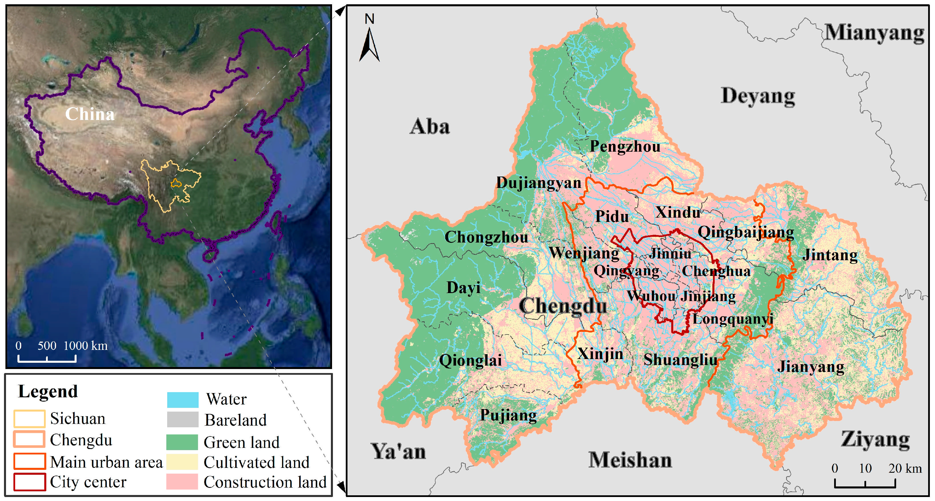
2.1.1. Study Area

Chengdu, the capital of Sichuan Province, serves as a key central city in southwest China. Positioned between 102°54′E and 104°53′E longitude and 30°05′N and 31°26′N latitude, it lies in the western Sichuan Basin and borders the eastern edge of the Tibetan Plateau. The city spans an area of 14,335 km², with the built-up area of the central urban area measuring 1063.68 km². Chengdu administers 20 districts, including 12 urban districts, 5 county-level cities, and 3 counties (Figure 1). The city has 1751 community committees and 1294 village committees [26]. As of the end of 2023, Chengdu’s permanent resident population had reached 21.403 million, an increase of 0.6% from the previous year, with an urbanization rate of 80.5%. The city’s GDP was CNY 2.20747 trillion in 2023 [27].

In recent years, rapid economic growth has driven the expansion and transformation of cities, with an increasing degree of urbanization. From 2015 to 2023, 97.93% of communities saw growth in their nighttime light (NTL) values, with 70.86% of communities experiencing a 100-fold increase. This significant growth reflects a substantial increase in urban nighttime vitality. Considering the differences in urban vitality between urban and suburban areas, this study focuses on the entire city of Chengdu, using 3046 communities (including community committees and village committees) as the main units of analysis. This approach helps to reveal more detailed regional vitality characteristics.

With the continuous development of multidimensional vitality theories, analyzing urban vitality from multiple perspectives has become increasingly accepted. For example, some areas may excel in vitality intensity but lack diversity (such as communities concentrated around commercial activities), while other areas may perform better in vitality diversity but have lower vitality intensity (such as residential areas and scenic spots). This situation highlights the necessity of depicting urban vitality from multiple angles and studying its spatial dynamics to identify the determining factors to formulate policies that promote future vitality.

2.1.2. Data Collection

This study examines the direct and indirect relationship between urban vitality and factors like transportation, amenities, and the natural environment by leveraging diverse and readily available remote sensing and open geographic datasets. These include community boundaries, points of interest (POI), NTL data, Land Use/Land Cover (LULC), normalized difference vegetation index (NDVI), building footprints, and others. To ensure the timeliness of the analysis, all data were collected between 2020 and 2024. The details of the data, including their names, acquisition times, sources, and types, are detailed in

Table 1. Data description.

Data Name	Data Source	Resolution (m)	Time (Year)	Type
Administrative boundary	Tianditu	-	2024	Vector
Bus station	AMAP	-	2024	Vector
Subway station	AMAP	-	2024	Vector
POI	AMAP	-	2022	Vector
River	OpenStreetMap	-	2024	Vector
Road	OpenStreetMap	-	2024	Vector
Building [28]	Zenodo	-	2020	Vector
Geohazard point	zldatas	-	2024	Vector
PM2.5 [29]	Zenodo	1000 × 1000	2023	Raster
Population	WorldPop	100 × 100	2020	Raster
LULC [30]	Esri Sentinel-2 Land cover	10 × 10	2020	Raster
NTL [5]	NPP/VIIRS	500 × 500	2023	Raster
NDVI [31]	National Ecosystem Science Data Center (NESDC)	30 × 30	2022	Raster
DEM	ASF ALOS	12.5 × 12.5	2022	Raster

Note: Tianditu (https://map.tianditu.gov.cn); AMAP (https://ditu.amap.com/); OpenStreetMap (https://www.openstreetmap.org/); Zenodo (https://zenodo.org/); WorldPop (https://www.worldpop.org/); zldatas (https://zldatas.com/); NPP/VIIRS (https://eogdata.mines.edu/products/vnl/) NESDC (http://www.nesdc.org.cn); ASF ALOS (https://search.asf.alaska.edu/#/). All data accessed on 1 January 2025.

.

Notably, a series of preprocessing steps, including geometry repair, typology processing, and the removal of duplicates and outliers using ArcGIS 10.8.1 and Python 3.8, were performed to maintain the data’s quality and consistency.

2.2. Urban Vitality Indicators

Urban vitality can be reflected through various indicators. Considering data availability and evaluation units, this study designed two dimensions—urban vitality intensity and urban vitality diversity—to comprehensively assess urban vitality and its influencing factors.

Urban vitality intensity refers to the magnitude or concentration of human and economic activities within an urban area. It quantifies the “activity” or “density” of the space, which are often measured through metrics such as NTL, population density (PD), and POI density (POID). VI reflects the “quantity” of urban vitality, emphasizing how much activity occurs in a given area. High VI typically correlates with urban cores, transportation hubs, or commercial districts.

Urban vitality diversity captures the functional heterogeneity and interaction within urban space. It measures the variety and balance of activities, functions, and land uses [32], which are often assessed using POI diversity (POIMD) and land use mix degree (LUMD) [33]. VD reflects the “quality” of urban vitality, emphasizing how diverse activities are and their potential for fostering social interaction, innovation, and resilience. High VD often occurs in mixed-use neighborhoods or areas with balanced residential–commercial integration. The higher the urban vitality diversity, the more integrated functions and interactions between people are present in the city, supporting a richer array of social and cultural activities.

2.3. Multidimensional Vitality-Related Factors

2.3.1. Variable Description

Urban vitality in a region is often closely related to various factors such as its natural environment, transportation environment, residential environment, and commercial facilities [34]. Therefore, we have designed an indicator system to assess urban vitality across five dimensions: commercial service (CS), public service (PS), transportation environment (TE), residential environment (RE), and natural environment (NE). These dimensions align with various facets of urban planning and management, offering enhanced decision-making support for city administrators.

Among the above variables, VI, VD, CS, PS, TE, RE, and NE cannot be directly obtained and need to be assessed using other measurable data. In structural equation modeling, unmeasurable variables are represented as latent variables, which are indicated by a set of observed variables that can be directly observed or measured [35]. The relationship between latent and observed variables follows a formative measurement model (FMM), meaning the meaning of latent variables is determined by the manifest variables, with manifest variables forming or causing latent variables.

Table 2. Description of variables.

Latent Variables	Observed Variables	Description	Unit	Data Source
Vitality intensity (VI)	PD	Population density	persons/km2	(a)
	NTL	Nighttime light value	nw/cm2/sr	(b)
	POID	POI density	POIs/km2	(c)
Vitality diversity (VD)	POIMD	POI mix degree	-	(c)
	LUMD	Land use mix degree	-	(d)
Commercial service (CS)	HA	POI density of surrounding hotel and accommodation services	POIs/km2	(c)
	DF	POI density of surrounding dining and food services	POIs/km2	(c)
	SS	POI density of surrounding shopping services	POIs/km2	(c)
Public service (PS)	SF	POI density of surrounding sports and fitness services	POIs/km2	(c)
	HC	POI density of surrounding healthcare services	POIs/km2	(c)
	EC	POI density of surrounding education and culture services	POIs/km2	(c)
Transportation environment (TE)	BSD	Bus station density	stations/km2	(e)
	DNSS	Distance to the nearest subway station	km	(f)
	RL	Length of roads per square kilometers	km/km2	(g)
	CD	Crossroad density	crossroads/km2	(g)
Residential environment (RE)	FAR	Floor area ratio	-	(h)
	ABH	Average building height	m	(h)
	BF	Building footprint	m2	(h)
Natural environment (NE)	NDVI	Normalized difference vegetation index	-	(i)
	GR	Green ratio	%	(d)
	PM2.5	PM2.5	μg/m3	(j)
	Slope	Slope		(k)
	GDD	Geological disaster density	events/km2	(l)

Note: (a) population; (b) NTL; (c) POI; (d) land cover; (e) bus station; (f) subway station; (g) road; (h) building; (i) NDVI; (j) PM2.5; (k) DEM; (l) geohazard point.

provides detailed descriptions and data sources for all latent and observed variables.

Commercial service is one of the core drivers of urban vitality. The distribution of commercial centers, dining, and hotel accommodation facilities directly impacts the frequency of activities and the intensity of economic activities within a region. High-density commercial facilities are typically associated with high foot traffic and high consumption, thereby enhancing the economic vitality of the city and the quality of life for residents. In this study, commercial service and public convenience are assessed by calculating the POI density of each community for the corresponding facility types.

Public service facilities, including those for education, healthcare, culture, and sports, directly affect residents’ quality of life. A well-developed public service network can promote social stability and development, increase residents’ sense of well-being, and enhance social participation, thereby boosting the social vitality and overall attractiveness of the city. Public service convenience is assessed by calculating the POI density of each community for the relevant types of public service facilities.

Transportation network is closely related to urban vitality. Convenient transportation infrastructure enhances the efficiency of people and goods movement, reduces geographical barriers, and factors such as city connectivity, commuting convenience, and traffic density all influence the strength of urban vitality. The density of bus stations, subway stations, road intersections, and road network density are calculated based on public transportation, subway, and road network data.

Residential environment quality directly relates to residents’ comfort, including factors such as residential density, floor area ratio (FAR), and building height [36]. The arrangement of buildings within a community offers important information about its level of congestion and economic vitality. To evaluate these aspects, the average building height, building footprint, and floor area ratio were computed for each community using building data [37].

Natural environment is an important factor influencing urban vitality. A healthy natural environment can improve residents’ physical and mental health, promote outdoor activities, and facilitate social interaction [38]. Flat terrain areas are conducive to urban expansion and infrastructure development. In this study, the natural environment is reflected through NDVI and greening rate (GR) [39], PM2.5 data to measure air quality, slope data to reflect topography, and geological disaster density (GDD) to assess the city’s natural disaster risk and safety.

2.3.2. Variable Calculation

To clarify the calculation methods, we categorized the observed variables based on their computational logic. Density metrics such as POID, HA, DF, SF, HC, EC, BSD, CD, and GDD were calculated as the ratio of the number of relevant points (e.g., POIs, bus stations) within a community to its area. Raster-based metrics, including PD, NTL, NDVI, GR, PM2.5, and slope, were derived by averaging the values of intersecting raster pixels. Diversity metrics (POIMD and LUMD) were quantified using the Shannon entropy index to reflect the mix of POI types or land use categories. Distance indicators (such as DNSS) are calculated as the geographical distance from the community boundary to the nearest subway station. Road and building metrics, such as RL (road length-to-area ratio), FAR (floor area ratio), ABH (average building height), and BF (building footprint ratio), were calculated using geometric and attribute data from vector layers.

Due to the varying magnitudes and units of the indicators, all observed variables were standardized using the Z-score normalization method. This approach transforms the data to a common scale with a mean of 0 and a standard deviation of 1, ensuring comparability across indicators while preserving their relative distributions.

$$y={\displaystyle \frac{y_{old}-\mu }{\sigma }}$$

(1)

where $y_{old}$ represents the original values, $\mu$ denotes the mean of the original values, and $\sigma$ is the standard deviation of the original values.

VI, VD, CS, PS, TE, RE, and NE are composite latent variables derived from reflectively measured indicators. The score of the latent variable is usually calculated by taking a weighted average of the observed variables, with the weights determined by the PLS algorithm to maximize the covariance between the latent variable and the observed variables. The calculation formula is as follows:

$$x={\displaystyle \sum _{i=1}^n\left(w_i\times y_i\right)}$$

(2)

where $n$ is the number of observed variables of latent variable $x$, $y_i$ denotes the value of observed variable; $w_i$ represents the outer weight of $y_i$, which are determined by the iteration of the PLS algorithm.

2.4. PLS-SEM

SEM is a statistical tool designed to model complex relationships between variables [40]. SEM enables the creation of latent factors from multiple observed indicators, facilitating a deeper understanding of the interrelationships among various components of complex systems [41]. PLS-SEM is an extension of SEM [42]. The reflective measurement model (RMM) and formative measurement model (FMM) in PLS-SEM helps mitigate multicollinearity issues common in ordinary least squares regression, making it particularly effective for datasets that do not adhere to a normal distribution [43]. Additionally, PLS-SEM is well-suited for studies with small or constrained sample size due to its strong predictive capabilities and its ability to effectively assess variable interactions [44].

Given that evaluating urban vitality using a single indicator is overly simplistic and that research samples often fail to conform to a normal distribution, this study constructed a comprehensive PLS-SEM model to simulate the complex relationships between two types of urban vitality indicators (VI and VD) as well as their influence factors, including CS, PS, TE, RE, and NE (Figure 2). The PLS-SEM model was then employed to investigate the relationships among latent variables. This approach enabled us to explore the interactions between urban vitality and its related factors, analyzing the mechanisms through which these multidimensional factors influence vitality via path coefficients and factor loadings. The PLS-SEM model is composed of two core components: the measurement model (outer model) and the structural model (inner model).

(1) The measurement model defines the associations between observed indicators and their corresponding latent constructs, as illustrated by all arrows in Figure 2, except those within the dashed boxes. The measurement equation is as follows:

$$y={\lambda }_{y}x+\epsilon$$

(3)

where ${\lambda }_y$ indicates the relationship between the latent variable $x$ and the observed variables $y$ through their factor loadings, and $\epsilon$ is the measurement error.

(2) The structural model shows the relationships between latent variables, represented by the arrows within the dashed boxes in Figure 2. In the structural model, latent variables serving as predictors are considered exogenous, while those representing outcomes are endogenous. The observation formula is as follows:

$$x=B\mu +\gamma \phi +\zeta$$

(4)

where $\mu$ represents the endogenous (dependent) latent variable, $\phi$ is the exogenous (independent) latent variable, and $B$ denotes the correlation among the endogenous latent variables. $\gamma$ is the exogenous latent variable that influences the endogenous latent variable, while $\zeta$ represents the portion of variance that cannot be explained by the model.

3. Results

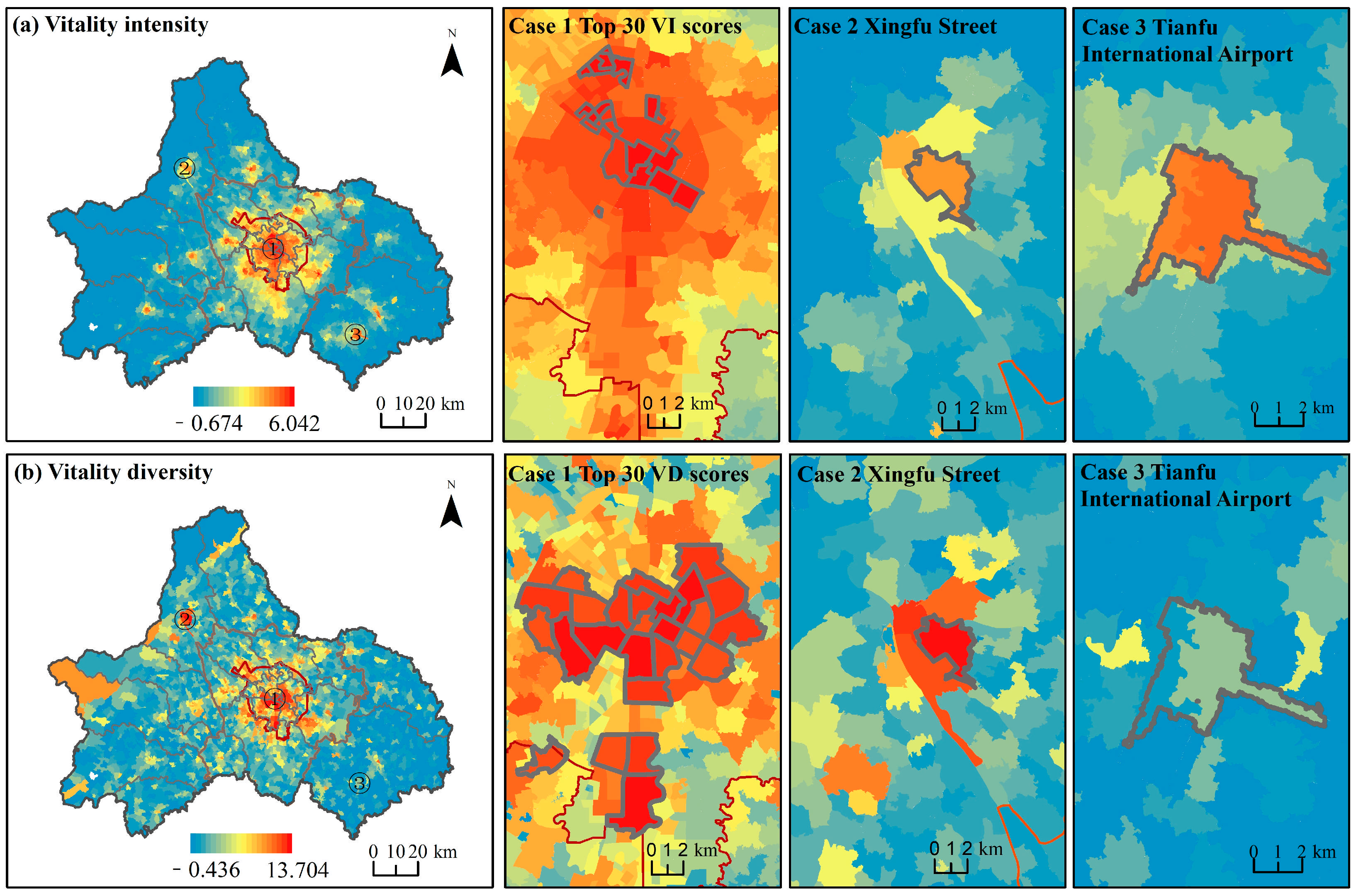
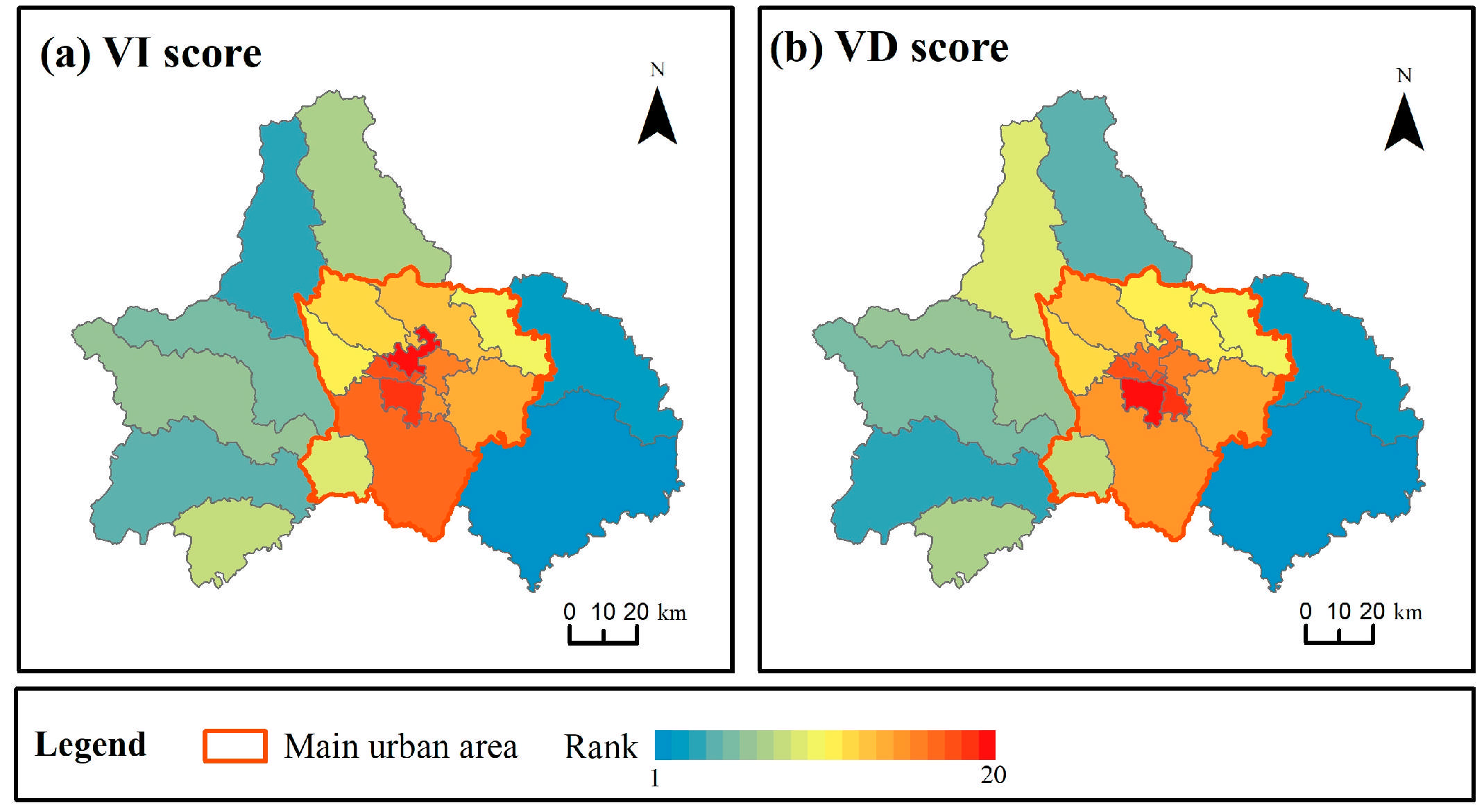
3.1. Urban Vitality in Chengdu

This study reveals the spatial distribution and differences in urban vitality intensity and vitality diversity across different communities in Chengdu. Figure 3 illustrates the spatial distribution of the scores for VI and VD, which are calculated by Equation (2). The central urban area (red line) and the main urban area (orange line) of Chengdu are highlighted based on the “Chengdu Land and Space Master Plan (2021–2035)”. Specifically, the central urban area intersects 11 districts, covering 4.84% of the city’s total area, and is the primary economic, political, and commercial hub of Chengdu. The main urban area includes 12 districts, covering 27.96% of the city’s total area.

To quantify observed spatial patterns, we employed Moran’s I to investigate the spatial autocorrelation characteristics of VI and VD. The computed Moran’s I values demonstrated distinct spatial aggregation patterns, with VI exhibiting stronger clustering (I = 1.12) compared to VD (I = 0.45). This statistically significant divergence (p < 0.01) indicates that both variables display positive spatial autocorrelation, though VI manifests more pronounced spatial dependency with neighboring values tending to cluster more intensely.

Delving into spatial specifics, high VI communities are mainly concentrated in the central urban area. Among the top 1% of the 30 highest VI communities, 15 are located in the Jinniu District, primarily within the Third Ring Road (Figure 3, case 1). Notably, commercial districts like Chunxi Road and Taikoo Li, which combine shopping, dining, and leisure, are representative of areas with high urban vitality intensity. Additionally, high- vitality communities are also scattered in the commercial centers of the main urban area and other districts, forming more than 10 high VI centers.

In contrast to VI, the spatial distribution of VD exhibits distinct characteristics. While similarly demonstrating clusters in the central urban area, the distribution of VD in peripheral regions diverges significantly from VI’s concentration pattern. Instead, it is more dispersed, with some medium to high VD communities located outside the commercial centers. A case in point includes the Tai’an community in Qingcheng Mountain Town, Yunhua village in Xiling Town, and Xingfu Street in Dujiangyan City (Figure 3, case 2), which are all situated in remote natural scenic areas. These exemplars generally have higher VD levels than VI, a phenomenon can be attributed to the high diversity of POI and land use in these areas, where residential, commercial, educational, cultural, and recreational facilities coexist. Conversely, urban centers (e.g., commercial districts) or transportation hubs (Chengdu Tianfu International Airport, Figure 3, case 3) typically display monocentric functional layouts, thereby yielding higher VI but comparatively lower VD.

3.2. Urban Vitality Related Factors

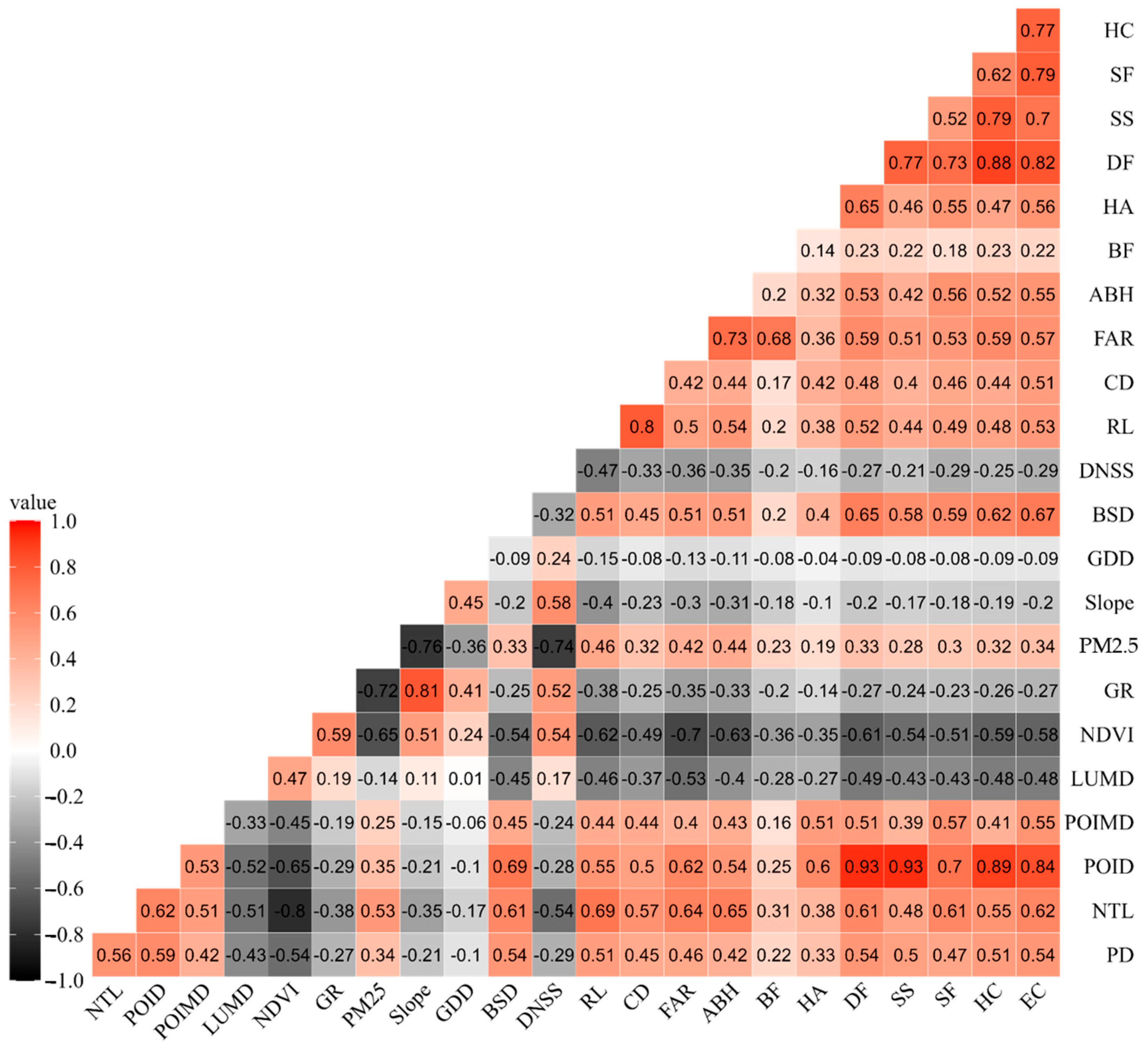
3.2.1. Correlation Analysis

The relationship between 23 observed indicators was analyzed using the Spearman correlation coefficient (Figure 4). The definitions and sources of all variables are provided in Table 2. The red and grey colors represent the strength of the correlation between variables, with grey indicating a negative correlation, red indicating a positive correlation, and darker colors indicating stronger correlations. All correlations are significant at the 0.05 level. From Figure 3, the following observations can be made.

The correlations between other observed variables and population density (PD), POI density (POID), and NTL are higher than those with the land use mix degree (LUMD) and POI mix degree (POIMD). Strong positive correlations (r > 0.56) were detected among PD, POID, and NTL, supporting their aggregation into the VI. This suggests that the VI is more clearly reflected by the observed variables, while it is more difficult to accurately explain VD through the observed variables.

The distance to subway stations (DNSS), NDVI, slope, greening rate (GR), disaster point density (GDD), and LUMD are negatively correlated with other observed variables, suggesting a negative relationship with both urban vitality intensity and vitality diversity. Among these, GDD shows a relatively low correlation with other positively correlated variables, with correlations below 0.15 for all variables except PM2.5.

The latent variable scores were calculated based on PLS using the observed variables. Figure 5 shows the Pearson correlation coefficients of latent variables in Model 1 (red squares) and Model 2 (green squares). The darker the color, the stronger the correlation. The results indicate that the correlation coefficients between variables are within the range of [−0.362, 0.872], suggesting a strong correlation between the latent variables, with the correlation in Model 1 being slightly higher than that of the same group of variables in Model 2.

Except for the NE, all other latent variables exhibit positive correlations. This is because areas with higher greening rates, NDVI, and slopes are typically located in suburban areas with relatively low population density. At the same time, these areas are characterized by scarce traffic environments, residential conditions, public services, and commercial facilities, leading to lower VI and VD. This suggests that, in most cases, it is difficult to reconcile the improvement of environmental quality with urban social development [45]. The correlation coefficient between CS and PS accessibility is greater than 0.8, indicating a strong correlation between the two. Part of this can be attributed to both sets of observed variables coming from the same data source, and the fact that POIs related to daily life are often located near POIs related to public services.

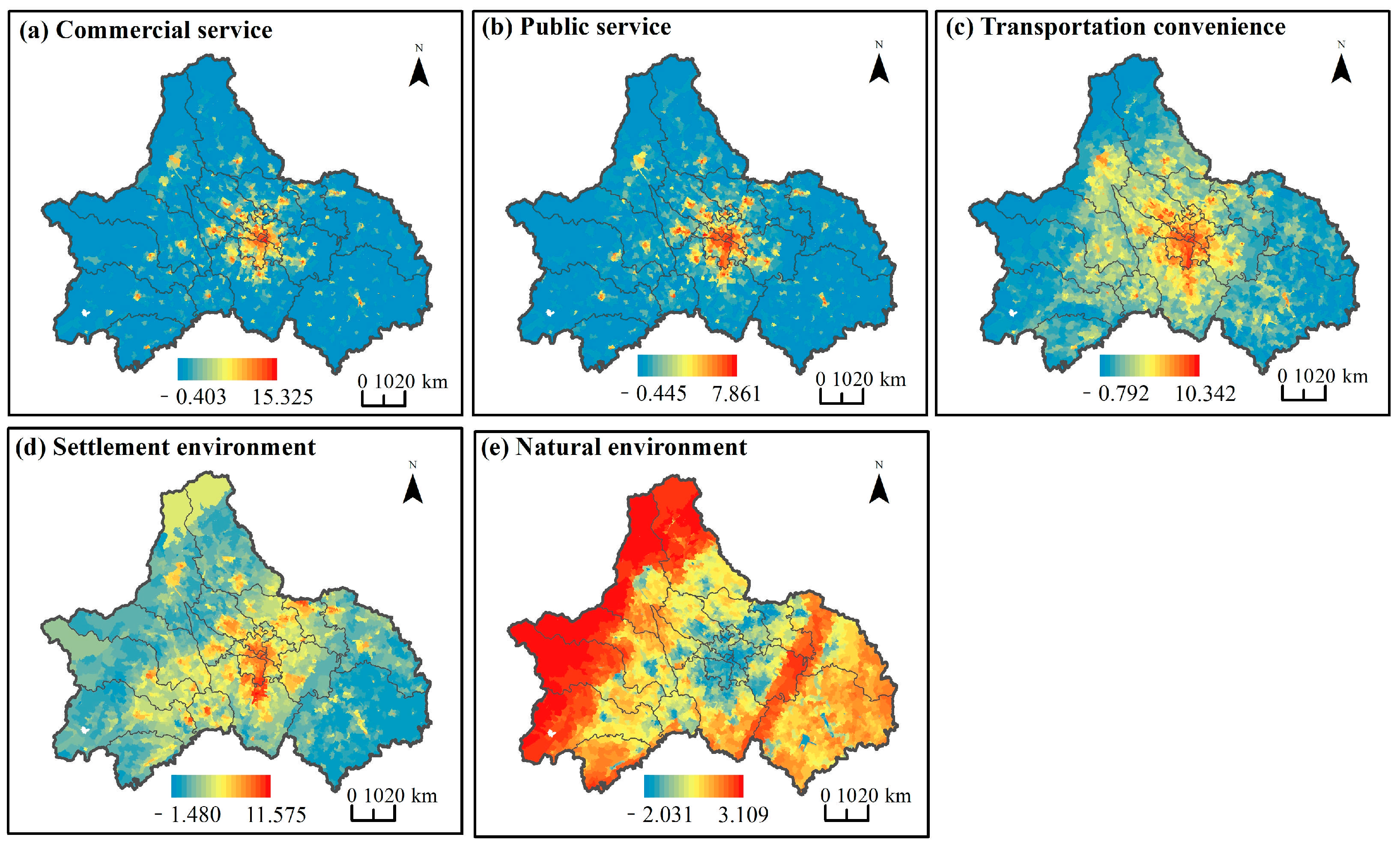
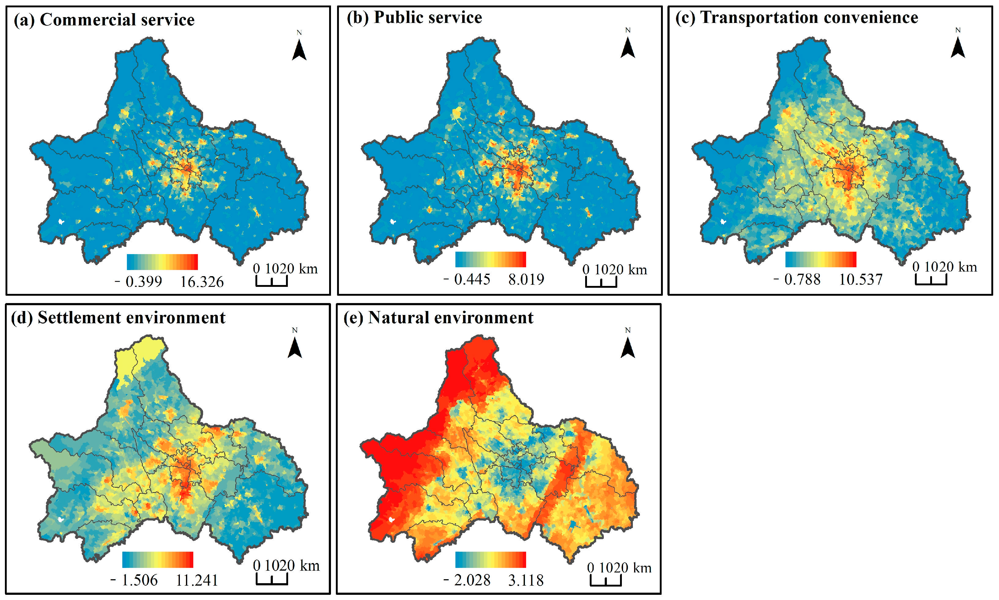
3.2.2. Spatial Distribution Features

To better analyze the factors influencing community vitality, spatial distribution maps are used to display the distribution of community scores for different latent variables including CS, PS, TC, RE, and NE. Figure 6 and Figure 7 show the spatial distribution of latent variable scores in Model 1 and Model 2, respectively. It can be observed that since the observed variables for the five independent variables (CS, PS, TC, RE, and NE) are the same, the latent variable scores and spatial distributions in Model 1 and Model 2 are very similar with a spatial correlation of 0.999. Figure 6 and Figure 7a–d exhibit similar multi-center distribution patterns, with a large cluster of high-value areas in the central urban area, and scattered high-value regions in the commercial centers of surrounding districts and counties. Additionally, the aggregation of commercial and public facilities is more evident, reflecting a more centralized distribution of POIs in the city. TC shows a stronger radial and connectivity pattern, forming a trend of outward radiation from the central urban area. Figure 6d and Figure 7d show that the RE scores in the High-tech District and Tianfu New District are higher than those in commercial centers like Chunxi Road, due to their higher floor area ratio and building height.

The spatial distribution pattern in Figure 6e and Figure 7e contrasts with the other four subgraphs. The city center, influenced by human activity, has a higher population density and typically exhibits lower NDVI and relatively insufficient per capita green space, which is negatively correlated with urban vitality, consistent with the model analysis results. Meanwhile, the NE scores align with the terrain and topography, with the Longmen Mountains on the western edge of the city and the Longquan Mountains in the western Sichuan Basin showing higher NE scores.

These results reveal the distribution characteristics of communities in Chengdu across different dimensions, reflecting disparities in infrastructure, traffic, and environmental factors within the region.

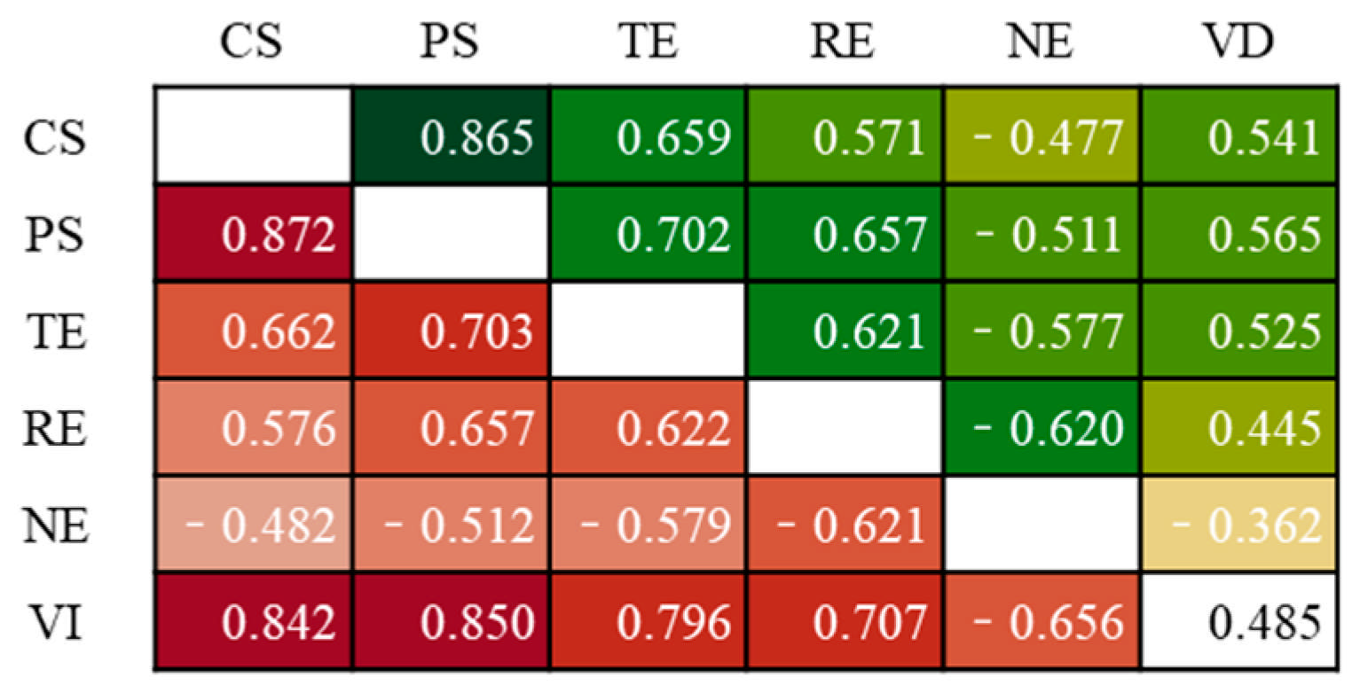
3.2.3. Association Mechanisms

Building on the correlation analysis results presented in Section 3.2.1, the connections between observed and latent variables were further explored (Figure 2). This study constructed Model 1 to analyze the factors related to VI and Model 2 to investigate the factors related to VD. The model results indicate that PM2.5, GDD, BF, and DNSS were not statistically significant and, therefore, were not suitable for measuring latent variables. These variables were excluded from the model. This outcome aligns with the weak correlations observed in the Spearman analysis (e.g., GDD showed correlations below 0.15 with most variables except PM2.5). The exclusion of these variables may stem from two factors. First, their limited explanatory power in reflecting urban vitality intensity and diversity could be attributed to spatial heterogeneity or non-linear interactions not captured by linear models. Second, the variables are weakly correlated, and their impact on urban vitality may be masked by other variables. Additionally, for 1 km PM2.5, grid data may not be able to capture subtle changes at the community level. These findings suggest that PM2.5, GDD, BF, and DNSS, while theoretically relevant, require more nuanced measurement approaches or contextual adjustments to enhance their empirical validity in future studies.

To comprehensively evaluate the quality and predictive capability of the PLS-SEM model, several indicators were used, including Cronbach’s $\alpha$, composite reliability (CR), average variance extracted (AVE), and correlation. The results are presented in

Table 3. PLS-SEM measured model.

Model	Crobach’s $\mathit{\alpha }$	CR	AVE	Correlation
Model 1
CS	0.834	0.900	0.752	0.842
PS	0.889	0.931	0.819	0.850
TC	0.808	0.886	0.723	0.796
RE	0.844	0.928	0.865	0.707
NE	0.839	0.889	0.728	−0.656
VI	0.913	0.888	0.726	1.000
Model 2
CS	0.834	0.901	0.754	0.541
PS	0.889	0.931	0.819	0.565
TC	0.808	0.887	0.723	0.525
RE	0.844	0.928	0.865	0.445
NE	0.839	0.889	0.729	−0.362
VD	—	—	—	1.000

Note: Composite reliability (CR) > 0.7; average variance extracted (AVE) > 0.5; correlation > 0.3.

. The CR values exceeded 0.7, indicating strong internal consistency of the latent variables and high reliability of the model. The AVE values were significantly greater than 0.5, suggesting that the latent variables explain more than 50% of the variance in their observed variables, indicating robust convergent validity. The correlations reflect the strength of the relationships between latent variables. In Model 1, the absolute values of the correlations were all greater than 0.65, indicating strong influences of CS, PS, TE, RE, and NE on VI, with the NE having a negative impact on VI. In Model 2, the absolute values of the correlations ranged from 0.35 to 0.60, with NE and RE showing moderate relationships with VD. In summary, the overall model fit indices fall within the ideal range, indicating that the model has good explanatory power in understanding urban vitality and demonstrates general validity.

Table 4. Path coefficients of the PLS-SEM model.

Latent Variables	Path Coefficient $\mathit{\beta }$		Observed Variables	Factor Loading
	VI	VD		VI	VD
CS	0.344	0.162	HA	0.767	0.790
			SS	0.879	0.863
			DF	0.947	0.944
PS	0.219	0.228	SF	0.876	0.884
			HC	0.891	0.882
			EC	0.946	0.947
TC	0.253	0.214	BSD	0.795	0.791
			CD	0.858	0.864
			RL	0.894	0.894
RE	0.106	0.069	ABH	0.923	0.928
			FAR	0.937	0.932
NE	−0.166	−0.002	Slope	0.799	0.800
			GR	0.854	0.854
			NDVI	0.904	0.904

presents the path coefficients and factor loadings for Model 1 and Model 2. Regarding the path coefficients, TE, RE, CS, and PS show significant positive correlations with VI, while NE exhibits a negative correlation with VI. This suggests that communities with higher VI and VD are typically located in areas with convenient transportation, and denser living conditions, but relatively poor natural environments. Additionally, high vitality and functionally diverse communities are generally associated with a higher density of living amenities, meaning that residents in these communities tend to enjoy better access to essential services.

This phenomenon may be explained through three interrelated mechanisms: Historical urban densification processes frequently emphasized transportation infrastructure and residential expansion at the expense of green space conservation. The economic value generated by vibrant urban zones could simultaneously reduce incentives for environmental improvement initiatives. Furthermore, the measurement framework’s capacity to quantify tangible urban amenities might outweigh its sensitivity to ecological quality assessments. This tension presents critical challenges for sustainable development: while high vitality improves access to services, environmental degradation could undermine long-term community health. Planners might address this through green infrastructure integration in high-density areas and revised zoning policies that balance built environment intensity with ecological preservation.

Regarding the factor loadings, both Model 1 and Model 2 have values greater than 0.7, indicating that the observed variables make a strong contribution to the latent variables.

4. Discussion

4.1. Divergent Mechanisms Between VI and VD

The comparative analysis reveals a notable divergence between Models 1 and 2: while VI exhibits strong correlations with five latent variables, VD demonstrates weaker explanatory power, as evidenced by the generally lower path coefficients in Model 2 (excluding public services). This pattern suggests that VI—reflecting a region’s overall activity level—serves as a more direct driver of urban development, whereas VD’s functional diversity appears to operate through indirect mechanisms.

There are several possible explanations for this observation. First, the indicators used to measure VD, such as POI diversity and land use diversity, might not fully capture the complexity of urban vitality diversity. Future research could explore additional indicators or more sophisticated methods to measure VD. Second, the relationship between VD and urban development might be more nuanced, potentially moderated by other factors such as urban planning policies or socioeconomic characteristics. Further studies could investigate these interactions to better understand the role of VD. Third, in the context of Chengdu, urban development might be more driven by dense activities rather than functional diversity, at least in the current stage of development [46]. As the city continues to evolve, the importance of VD may increase, making it a more significant factor in future research.

In summary, while VI appears to be a stronger predictor in our current analysis, VD remains an important dimension of urban vitality that should be considered in urban planning and policy-making to foster sustainable and vibrant urban spaces.

4.2. Balancing Urban Vitality for Sustainable Development

Urban planning and development should consider both vitality intensity and diversity. For example, the central urban area consistently leads in both vitality intensity and diversity, making it the most vibrant; while some tourist areas farther from the city center exhibit higher VD relative to VI. To enhance the intensity and diversity of community vitality, urban managers can formulate policies across multiple dimensions, including the natural environment, transportation, and public facilities [3].

Using the community VI and VD scores, the average VI and VD values for each district were calculated. Figure 8 displays the distribution and differences in VI and VD characteristics across districts. It is evident that the districts do not exhibit consistent rankings in terms of urban vitality intensity and diversity. For instance, Jinniu District has the highest urban vitality, owing to its high density of real estate development and population, while Wuhou District has the highest vitality diversity, benefiting from its rich cultural and historical heritage, as well as the presence of multiple higher education institutions and research organizations. Additionally, we conducted a correlation analysis between the VI, VD values, and per capita GDP for each district. The correlations were 0.851 and 0.837, respectively, indicating a close relationship between urban vitality and local economic development. This result suggests that enhancing urban vitality may be crucial for economic prosperity and citizen well-being.

The results in Figure 5 indicate that improving the urban environmental quality in synergy with other factors can significantly enhance overall urban vitality and promote sustainable urban development. The results in Figure 4 help local governments identify gaps in urban vitality, differences from other communities, and future priorities for community management. Moreover, increasing vitality and diversity requires multi-dimensional collaboration and action, including urban governance and legislation, infrastructure development, education improvement, climate change adaptation, and harmonious coexistence with nature [7,47]. Overall, urban vitality is essential for achieving sustainable urban development.

4.3. Limitations and Future Research

The PLS-SEM approach has been validated in Chengdu and has great potential for application to cities with similar urban challenges. Key prerequisites include (1) the availability of multi-source spatiotemporal data (e.g., POIs, mobile signals, satellite imagery); (2) administrative boundaries at the neighborhood level; and (3) contextual calibration of variables (e.g., adjusting POI categories to reflect local functional priorities). For example, in cities with informal settlements, integrating crowdsourced data (e.g., OpenStreetMap) can fill gaps in official datasets.

Despite its potential, this study has several limitations that warrant discussion and future exploration, with the first being: (1) data and indicator constraints. The current framework does not incorporate critical economic factors (e.g., regional GDP, income distribution, employment rates), potentially limiting a holistic understanding of vitality drivers. Furthermore, reliance on static data restricts insights into temporal dynamics, such as diurnal/weekly vitality fluctuations or long-term trends. To address this, future work should integrate dynamic datasets (e.g., real-time mobility flows, longitudinal economic statistics) and employ time-series analyses to model vitality evolution.

(2) Methodological limitations: While PLS-SEM is useful for handling complex models with small samples and non-normal data, it is primarily correlation-based and identifies associations rather than causal relationships. Furthermore, our study found significant spatial clustering in urban vitality, where nearby areas tend to exhibit similar vitality levels. However, PLS-SEM does not account for spatial autocorrelation, which could bias the estimated relationships due to violations of the assumption of independence. Future research could address this by using spatial regression models to better capture spatial dependencies and provide a more accurate assessment of urban vitality factors.

(3) Unaddressed vitality dimensions: Urban aesthetics (e.g., architectural harmony, sky view factor) and morphology (e.g., street network connectivity, building height diversity) are critical yet omitted due to data and methodological gaps. In future studies, we will explore advanced techniques such as street-view imagery analysis and 3D urban modeling to systematically integrate these dimensions.

5. Conclusions

This study advances community-level urban vitality assessment by integrating multisource spatiotemporal data and a PLS-SEM framework, revealing two core insights. First, urban vitality intensity and diversity exhibit distinct spatial patterns: VI clusters in population-dense areas with well-developed commercial facilities but relatively poor natural environments, while VD peaks in communities with balanced land use and POI. Second, multidimensional factors differentially influence VI and VD. VI is predominantly driven by CS and TE, whereas VD is most affected by PS and TE. Notably, RE and NE had minimal effects on VD.

Compared to prior studies, this work makes two key contributions. First, it provides a multidimensional understanding of vitality by analyzing both intensity and diversity dimensions through statistical and spatial characteristics. Second, it clarifies the interactions among multidimensional drivers of vitality, advancing the comprehension of its complex relationships. These findings bridge data-driven urban analytics with planning practice, offering actionable insights for sustainable community development.

References

1. Chen, Y.; Yu, B.; Shu, B.; Yang, L.; Wang, R. Exploring the spatiotemporal patterns and correlates of urban vitality: Temporal and spatial heterogeneity. Sustain. Cities Soc. 2023, 91, 104440. [Google Scholar] [CrossRef]
2. Zhou, L.; Yuan, B.; Hu, F.; Wei, C.; Dang, X.; Sun, D. Understanding the effects of 2D/3D urban morphology on land surface temperature based on local climate zones. Build. Environ. 2022, 208, 108578. [Google Scholar] [CrossRef]
3. Mouratidis, K.; Poortinga, W. Built environment, urban vitality and social cohesion: Do vibrant neighborhoods foster strong communities? Landsc. Urban Plan. 2020, 204, 103951. [Google Scholar] [CrossRef]
4. Zografos, C.; Klause, K.A.; Connolly, J.J.; Anguelovski, I. The everyday politics of urban transformational adaptation: Struggles for authority and the Barcelona superblock project. Cities 2020, 99, 102613. [Google Scholar] [CrossRef]
5. Maas, P.R. Towards a Theory of Urban Vitality; University of British Columbia: Vancouver, BC, Canada, 1984. [Google Scholar]
6. Smith, T.; Nelischer, M.; Perkins, N. Quality of an urban community: A framework for understanding the relationship between quality and physical form. Landsc. Urban Plan. 1997, 39, 229–241. [Google Scholar] [CrossRef]
7. Liu, H.; Gou, P.; Xiong, J. Vital triangle: A new concept to evaluate urban vitality. Comput. Environ. Urban Syst. 2022, 98, 101886. [Google Scholar] [CrossRef]
8. Li, S.; Chen, P.; Hui, F.; Gong, M. Evaluating urban vitality and resilience under the influence of the COVID-19 pandemic from a mobility perspective: A case study in Shenzhen, China. J. Transp. Geogr. 2024, 117, 103886. [Google Scholar] [CrossRef]
9. Zhang, A.; Xia, C.; Chu, J.; Lin, J.; Li, W.; Wu, J. Portraying urban landscape: A quantitative analysis system applied in fifteen metropolises in China. Sustain. Cities Soc. 2019, 46, 101396. [Google Scholar] [CrossRef]
10. Kim, Y.-L. Data-driven approach to characterize urban vitality: How spatiotemporal context dynamically defines Seouls nighttime. Int. J. Geogr. Inf. Sci. 2020, 34, 1235–1256. [Google Scholar] [CrossRef]
11. Liu, M.; Jiang, Y.; He, J. Quantitative evaluation on street vitality: A case study of Zhoujiadu community in Shanghai. Sustainability 2021, 13, 3027. [Google Scholar] [CrossRef]
12. Yue, W.; Chen, Y.; Zhang, Q.; Liu, Y. Spatial explicit assessment of urban vitality using multi-source data: A case of Shanghai, China. Sustainability 2019, 11, 638. [Google Scholar] [CrossRef]
13. Martí, P.; Serrano-Estrada, L.; Nolasco-Cirugeda, A. Social media data: Challenges, opportunities and limitations in urban studies. Comput. Environ. Urban Syst. 2019, 74, 161–174. [Google Scholar] [CrossRef]
14. Zhang, Z.; Liu, J.; Wang, C.; Zhao, Y.; Zhao, X.; Li, P.; Sha, D. A spatial projection pursuit model for identifying comprehensive urban vitality on blocks using multisource geospatial data. Sustain. Cities Soc. 2024, 100, 104998. [Google Scholar] [CrossRef]
15. Guo, X.; Chen, H.; Yang, X. An evaluation of street dynamic vitality and its influential factors based on multi-source big data. ISPRS Int. J. Geo-Inf. 2021, 10, 143. [Google Scholar] [CrossRef]
16. Tu, W.; Zhu, T.; Xia, J.; Zhou, Y.; Lai, Y.; Jiang, J.; Li, Q. Portraying the spatial dynamics of urban vibrancy using multisource urban big data. Comput. Environ. Urban Syst. 2020, 80, 101428. [Google Scholar] [CrossRef]
17. Wang, Z.; Xia, N.; Zhao, X.; Gao, X.; Zhuang, S.; Li, M. Evaluating Urban Vitality of Street Blocks Based on Multi-Source Geographic Big Data: A Case Study of Shenzhen. Int. J. Environ. Res. Public Health 2023, 20, 3821. [Google Scholar] [CrossRef]
18. Jiang, Y.; Huang, Z.; Zhou, X.; Chen, X. Evaluating the impact of urban morphology on urban vitality: An exploratory study using big geo-data. Int. J. Digit. Earth 2024, 17, 2327571. [Google Scholar] [CrossRef]
19. Pan, H.; Yang, C.; Quan, L.; Liao, L. A new insight into understanding urban vitality: A case study in the Chengdu-Chongqing area twin-city economic circle, China. Sustainability 2021, 13, 10068. [Google Scholar] [CrossRef]
20. Wang, Z.; Wang, X.; Liu, Y.; Zhu, L. Identification of 71 factors influencing urban vitality and examination of their spatial dependence: A comprehensive validation applying multiple machine-learning models. Sustain. Cities Soc. 2024, 108, 105491. [Google Scholar] [CrossRef]
21. Xiao, Z.; Li, C.; Pan, S.; Wei, G.; Tian, M.; Hu, R. Exploring the Spatial Impact of Multisource Data on Urban Vitality: A Causal Machine Learning Method. Wirel. Commun. Mob. Comput. 2022, 1, 5263376. [Google Scholar] [CrossRef]
22. Liu, S.; Zhang, L.; Long, Y. Urban vitality area identification and pattern analysis from the perspective of time and space fusion. Sustainability 2019, 11, 4032. [Google Scholar] [CrossRef]
23. Ye, Y.; Li, D.; Liu, X. How block density and typology affect urban vitality: An exploratory analysis in Shenzhen, China. Urban Geogr. 2018, 39, 631–652. [Google Scholar] [CrossRef]
24. Najaf, P.; Thill, J.-C.; Zhang, W.; Fields, M.G. City-level urban form and traffic safety: A structural equation modeling analysis of direct and indirect effects. J. Transp. Geogr. 2018, 69, 257–270. [Google Scholar] [CrossRef]
25. Fan, Y.; Chen, J.; Shirkey, G.; John, R.; Wu, S.R.; Park, H.; Shao, C. Applications of structural equation modeling (SEM) in ecological studies: An updated review. Ecol. Process. 2016, 5, 19. [Google Scholar] [CrossRef]
26. Chengdu Yearbook Society. Chengdu Yearbook; Chengdu Yearbook Press: Chengdu, China, 2022. [Google Scholar]
27. Chengdu Municipal Statistics Bureau. The 2023 Chengdu Statistical Bulletin of National Economic and Social Development; Chengdu Municipal Statisties Bureau: Chengdu, China, 2023. [Google Scholar]
28. Che, Y.; Li, X.; Liu, X.; Wang, Y.; Liao, W.; Zheng, X.; Zhang, X.; Xu, X.; Shi, Q.; Zhu, J.; et al. 3D-GloBFP: The first global three-dimensional building footprint dataset. Earth Syst. Sci. Data 2024, 16, 5357–5374. [Google Scholar] [CrossRef]
29. Wei, J.; Li, Z.; Lyapustin, A.; Sun, L.; Peng, Y.; Xue, W.; Su, T.; Cribb, M. Reconstructing 1-km-resolution high-quality PM2.5 data records from 2000 to 2018 in China: Spatiotemporal variations and policy implications. Remote Sens. Environ. 2021, 252, 112136. [Google Scholar] [CrossRef]
30. Karra, K.; Kontgis, C.; Statman-Weil, Z.; Mazzariello, J.C.; Mathis, M.; Brumby, S.P. Global land use/land cover with Sentinel 2 and deep learning. In Proceedings of the 2021 IEEE International Geoscience and Remote Sensing Symposium IGARSS, Brussels, Belgium, 11–16 July 2021; pp. 4704–4707. [Google Scholar]
31. Yang, J.; Dong, J.; Xiao, X.; Dai, J.; Wu, C.; Xia, J.; Zhao, G.; Zhao, M.; Li, Z.; Zhang, Y.; et al. Divergent shifts in peak photosynthesis timing of temperate and alpine grasslands in China. Remote Sens. Environ. 2019, 233, 111395. [Google Scholar] [CrossRef]
32. Duan, J.; Wang, H.; Liu, L.; Zhang, J. The attraction gradient of urban functions: How does functional mix at multiple scales predict urban vitality. Cities 2025, 156, 105516. [Google Scholar] [CrossRef]
33. Zhou, L.; Wei, L.; López-Carr, D.; Dang, X.; Yuan, B.; Yuan, Z. Identification of irregular extension features and fragmented spatial governance within urban fringe areas. Appl. Geogr. 2024, 162, 103172. [Google Scholar] [CrossRef]
34. Doan, Q.C.; Ma, J.; Chen, S.; Zhang, X. Nonlinear and threshold effects of the built environment, road vehicles and air pollution on urban vitality. Landsc. Urban Plan. 2025, 253, 105204. [Google Scholar] [CrossRef]
35. Wang, C.; Ma, L.; Zhang, Y.; Chen, N.; Wang, W. Spatiotemporal dynamics of wetlands and their driving factors based on PLS-SEM: A case study in Wuhan. Sci. Total Environ. 2022, 806, 151310. [Google Scholar] [CrossRef] [PubMed]
36. Jin, A.; Ge, Y.; Zhang, S. Spatial Characteristics of Multidimensional Urban Vitality and Its Impact Mechanisms by the Built Environment. Land 2024, 13, 991. [Google Scholar] [CrossRef]
37. Zhan, D.; Kwan, M.-P.; Zhang, W.; Fan, J.; Yu, J.; Dang, Y. Assessment and determinants of satisfaction with urban livability in China. Cities 2018, 79, 92–101. [Google Scholar] [CrossRef]
38. Chen, M.; Cai, Y.; Guo, S.; Sun, R.; Song, Y.; Shen, X. Evaluating implied urban nature vitality in San Francisco: An interdisciplinary approach combining census data, street view images, and social media analysis. Urban For. Urban Green. 2024, 95, 128289. [Google Scholar] [CrossRef]
39. Goward, S.N.; Markham, B.; Dye, D.G.; Dulaney, W.; Yang, J. Normalized difference vegetation index measurements from the advanced very high resolution radiometer. Remote Sens. Environ. 1991, 35, 257–277. [Google Scholar] [CrossRef]
40. Jöreskog, K.G. A general approach to confirmatory maximum likelihood factor analysis. Psychometrika 1969, 34, 183–202. [Google Scholar] [CrossRef]
41. Leguina, A. A primer on partial least squares structural equation modeling (PLS-SEM). Int. J. Res. Method Educ. 2015, 38, 220–221. [Google Scholar] [CrossRef]
42. Hair, J.F.; Ringle, C.M.; Sarstedt, M. Partial least squares structural equation modeling: Rigorous applications, better results and higher acceptance. Long Range Plan. 2013, 46, 1–12. [Google Scholar] [CrossRef]
43. Hair, J.F.; Sarstedt, M.; Ringle, C.M.; Mena, J.A. An assessment of the use of partial least squares structural equation modeling in marketing research. J. Acad. Mark. Sci. 2012, 40, 414–433. [Google Scholar] [CrossRef]
44. Chao, Y.; Gao, L.; Liu, Y.; Yang, N.; Lyu, X.; Zhang, Y.; Guan, Q. Multi-perspective perception of urban relative poverty and its associated factors analysis: A case study of Wuhan City. Cities 2024, 153, 105320. [Google Scholar] [CrossRef]
45. Busch, J.; Amarjargal, O. 100 global bright spots of green growth: Co-occurrence of nighttime light gain and forest gain, 1990–2015. Glob. Environ. Chang. 2022, 75, 102556. [Google Scholar] [CrossRef]
46. Li, Q.; Cui, C.; Liu, F.; Wu, Q.; Run, Y.; Han, Z. Multidimensional Urban Vitality on Streets: Spatial Patterns and Influence Factor Identification Using Multisource Urban Data. ISPRS Int. J. Geo-Inf. 2021, 11, 2. [Google Scholar] [CrossRef]
47. Folke, C.; Polasky, S.; Rockström, J.; Galaz, V.; Westley, F.; Lamont, M.; Scheffer, M.; Österblom, H.; Carpenter, S.R.; Chapin, F.S., III; et al. Our future in the Anthropocene biosphere. Ambio 2021, 50, 834–869. [Google Scholar] [CrossRef] [PubMed]
Figure 1. Study area map of Chengdu, showing districts (Wuhou, Jinniu, Chenghua, Jinjiang, Qingyang, Longquanyi, Qingbaijiang, Xindu, Pidu, Wenjiang, Xinjin, and Shuangliu), counties (Pujiang, Jintang, and Dayi), and county-level cities (Pengzhou, Dujiangyan, Chongzhou, Qionglai, and Jianyang).
Remotesensing 17 01056 g001
Figure 2. PLS-SEM model of urban vitality-related factors.
Remotesensing 17 01056 g002
Figure 3. Spatial distribution of VI and VD scores: ➀ case 1; ➁ case 2; ➂ case 3. (a) Vitality intensity; (b) vitality diversity. Case 1: Top 30 communities with the highest VI/VD scores within the Third Ring Road. Case 2: Xingfu Street in Dujiangyan City. Case 3: Chengdu Tianfu International Airport.
Remotesensing 17 01056 g003
Figure 4. Spearman’s correlation between variables.
Remotesensing 17 01056 g004
Figure 5. Correlations between latent variable scores.
Remotesensing 17 01056 g005
Figure 6. Latent variable score of Model 1. (a) Commercial service; (b) public service; (c) transportation convenience; (d) settlement environment; (e) natural environment.
Remotesensing 17 01056 g006
Figure 7. Latent variable score of Model 2. (a) Commercial service; (b) public service; (c) transportation convenience; (d) settlement environment; (e) natural environment.
Remotesensing 17 01056 g007
Figure 8. VI and VD scores of districts. (a) VI score; (b) VD score.
Remotesensing 17 01056 g008