Abstract
This paper presents a comparison of different image fusion methods for matching visible-spectrum images with thermal-spectrum (far-infrared) images, aimed at enhancing person detection using convolutional neural networks (CNNs). While object detection with RGB images is a well-developed area, it is still greatly limited by lighting conditions. This limitation poses a significant challenge in image detection playing a larger role in everyday technology, where illumination cannot always be controlled. Far-infrared images (which are partially invariant to lighting conditions) can serve as a valuable complement to RGB images in environments where illumination cannot be controlled and robust object detection is needed. In this work, various early and middle fusion techniques are presented and compared using different multispectral datasets, with the aim of addressing these limitations and improving detection performance.
1. Introduction
Object detection is already an extensively studied field that has yielded impressive results. However, most of the work has focused on visible-spectrum images captured with conventional cameras, which present inherent limitations. Certain applications require a level of robustness beyond what can be achieved with standard RGB images. Tasks such as search-and-rescue (SAR) operations and security and surveillance applications cannot rely on controlled lighting conditions and need to remain robust across different scenarios.
In the last decade, two families of detectors based on convolutional neural networks (CNNs)have dominated the field. One family is based on two-stage object detectors such as RCNN [1] and its successors, Fast-RCNN [2] and Faster-RCNN [3]. In the second family of one-stage object detectors, the YOLO [4] algorithm and its different versions stand out. In recent years, transformer architectures, initially proposed by [5], have been incorporated into object detection as a stand-alone approach, such as DETR [6]. Research has continued to push forward in optimizing the training process, reducing model complexity, improving scalability, enhancing precision, increasing detection speed, and refining many other features, but it has usually focused on visible-spectrum images.
But what happens when conditions cannot be controlled? What happens when occlusions or objects obscure the target objects that need to be detected? SAR operations and security applications are expected to operate continuously and in real time under unknown and uncontrolled conditions. A straightforward application could be an autonomous system onboard a mobile robot or UAV. While a robot can change perspectives or even deal with certain challenging lighting conditions, there are still cases where it would be impossible to achieve good performance with only visible-spectrum information. One such edge case is shown in Figure 1c, but there are many other similar situations. Although the person cannot be detected at all in the visible-spectrum image, they are clearly recognizable in the thermal image. The opposite scenario is also possible.
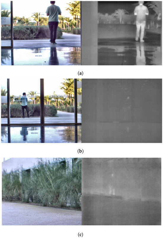
Figure 1.
Visible and thermal image pairs under different conditions: (a) Visible and thermal images under normal conditions. (b) Visible and thermal images of a person behind glass doors. (c) Visible and thermal images of a person behind bushes.
Thermal cameras are able to detect infrared radiation, which is proportional to an object’s temperature. Depending on the range of temperatures measured, different spectra can be used. The infrared or thermal spectrum is usually divided into different ranges: visible (VIS), near-infrared (NIR), short-wave infrared (SWIR), and long-wave infrared (LWIR). Higher temperatures can be better measured at shorter wavelengths, whereas these temperatures might cause a noisy image at longer wavelengths such as LWIR [7], which is a better alternative for lower temperatures [8]. For typical SAR operations or security applications, the most suitable spectrum ranges from 8 µm to 14 µm, known as far-infrared or long-wave infrared (LWIR), which have proven to be reliable spectra for measuring human temperatures [9]. They are also valuable in Earth science research, as they allow for monitoring surface temperatures [10], and they are useful in wildlife well-being and thermoregulatory behavior studies [11]. Depending on the camera sensor’s sensitivity, it is possible to capture temperatures between −20 °C and 1000 °C. For temperatures ranging from −10 °C to 130 °C, measurements can be taken with an LWIR camera [12] without any cooling equipment and without overstressing the camera sensor, making it a perfect solution for this kind of use case.
Some approaches rely solely on thermal images, as demonstrated in [13] or [14], which were evaluated using YOLOv3. YOLOv3 is a one-stage detector, initially introduced in [15], and forms the foundation for understanding the current development of the YOLO family. While thermal imagery offers rich data that are invariant to lighting conditions, it still has some limitations, such as the presence of transparent objects in the visible spectrum that may not be detectable in thermal images. It is also susceptible to climatological conditions, such as changes in ambient temperature or variations in human clothing. These aspects pose clear challenges for detection tasks.
It is important to differentiate calibrated from non-calibrated thermal cameras. Some available thermal cameras are previously calibrated so that the temperature of each specific pixel can be inferred from the gray level of the corresponding image. Other models, despite not being calibrated, still have a constant exposure time. In this way, the temperature-to-gray-value match remains constant across all images. Finally, some cameras include autoexposure or contrast enhancements that might worsen the impact of different climatological conditions on the dataset. In the specific case of this research (person detection), any of the mentioned camera types should provide better results by maintaining a coherent gray-level representation of people in different background conditions (warm or cold, depending on climatological conditions).
Since each type of image (visible and thermal) has its own strengths and weaknesses, a promising solution could involve fusing the information from both images. Under nominal conditions, the person should appear in both images, as in the case shown in Figure 1a; however, as shown in Figure 1b or Figure 1c, even though the person is recognizable in one spectrum, they may not be visible in the other. There are different approaches to this problem, the first being to merge both images before introducing the information to the detection algorithm (usually based on deep learning), also known as early fusion. The fusion of images can range from easy solutions, such as averaging time channels [16], to more complex solutions, such as superpixel segmentation, as in the approach presented in [17]; wavelet transforms [18]; or wavelet analysis in RGB-NIR image fusion [19]. Other works, focused on detecting moving wildlife, such as [20], follow a different approach, using airborne images to fuse different thermal images with a visible image so that moving parts are highlighted in different colors. Using a deep network to learn the fusion of images is also an interesting approach, either by integrating it into the feature extraction stage [21,22], using attention mechanisms [23], or applying it in the classification/detection stage. In cases where thermal and visible images do not match, a depth estimation module is needed beforehand to reproject the information [24].
When exploring new solutions for this problem, as stated in the Introduction, it is always tempting to delve into the latest state-of-the-art techniques, often involving complex architectures and methodologies. However, before doing so, it is crucial to establish a solid baseline that ensures not only the performance of different algorithms but also the quality of the input data to be used. A basic approach is to compare different techniques, and if their complexity is really worth their use. This research focuses on early fusion algorithms to verify how robustly simple approaches can perform before resorting to more complex methodologies. This manuscript also emphasizes the importance of the input data, evaluating some approaches that could enhance their quality or at least point out their limitations to be addressed in future research.
Even though making use of both RGB and thermal images has already proved to be useful in SAR missions, such as in [25], there is still work required before this approach can take full advantage of the benefits of automation [26]. The contributions of this paper include a comparison between four early fusion approaches and three middle fusion detection algorithms based on CNNs, based on matching visual–thermal images, and how the range restriction problem can affect them, with a proposed solution. The impact of unsynchronized image pairs is also explored, proposing a feasible solution to this problem. A CNN deep learning algorithm was used to assess the performance of each of them based on a fully autonomous approach.
The remainder of this paper is structured as follows: Section 2 covers the methodology used in the performance analysis, presenting the detection algorithm, the dataset as well as its characteristics and limitations, and with the training approach. The different image fusion methods, both early and middle fusion approaches, are described in Section 3. In Section 4, the results of the different tests with different datasets are discussed. These results are provided in Section 5, with the conclusions and proposed future research.
For reproducibility purposes, the source code of this implementation is publicly available (https://github.com/enheragu/yolo_test_utils, accessed on 26 February 2025).
2. Methodology
This section describes different aspects about the methodology followed in this research, the motivation behind the decisions taken, and a thorough explanation of how the experiments could be replicated.
2.1. The Detection Algorithm
In this experiment, the detection algorithm was mainly used as a constant descriptor to evaluate the different fusion methods proposed. In the specific use case proposed in this manuscript, i.e., SAR operations and similar use cases, the system should run onboard a mobile robot or UAV where memory and energy consumption are limited. A one-stage detector such as YOLOv8 has been proven to be faster than others such as Faster R-CNN [3] or DETR [6]. YOLOv8 provides notable results while maintaining controlled memory consumption. While YOLOv8 (m size) operates with around 25 M parameters, other SOTA algorithms such as Faster R-CNN make use of 35 M of parameters, ResNetSt-200 [27] requires 70 M of parameters, and others use up to 304 M parameters (Co-DETR proposed in [28]). YOLOv8 offers a low-memory, high-speed solution ideal for real-time, onboard deployment on resource-limited platforms.
YOLOv8
The final version used in this study is based on YOLOv8, as presented in [29]. Although YOLOv8 provides functionalities such as classification, segmentation, and detection, only the detection stack was used.
Taking a three-channel input image, YOLOv8 detects objects by providing their position, class, and bounding box dimensions. In this case, YOLOv8 was trained to detect only one class: person.
YOLOv8 handles image detection (positive or negative) with two confidence metrics: box confidence and class confidence. Box confidence combines objectness score (does the box contains an object?) and intersection over union (IoU). Class confidence is the conditional probability of the class given that an object is detected. IoU was configured as 0.5, as recommended by [30]. The class confidence varies in a continuous range and, as most of the metrics that are later explained, is a function of this parameter.
2.2. Data
As already stated, this research focused on the detection problem with multispectral images (visible and thermal from far-infrared spectrum). To tackle this problem, multispectral aligned images with a pixel-to-pixel match are needed. The FLIR-ADAS dataset is a good resource, although it only contains thermal information [31]. CVC-14, which includes multispectral images (visible and thermal), has issues with the rectification between images, as reported by [32]. The LLVIP dataset [33], captured with a similar approach as the one followed in CVC-14, tackles the misalignment and rectification problem, providing a robust dataset. Another well-explored dataset in the literature is the KAIST dataset [34]. KAIST also includes calibrated image pairs in both the visible and thermal spectra. Finally, the Multi-spectral Object Detection Dataset [35] includes labeled image pairs with multiple objects. Images and data from other datasets reported in the literature could not be found and are not mentioned here. Based on the information provided, the tests focused on both the LLVIP and KAIST datasets, which include labeled image pairs (for pedestrians) in the needed spectra. The following sections focus on describing both datasets and how they were used in the tests performed.
2.2.1. KAIST Dataset
The images used in this evaluation were all extracted from the published KAIST dataset, presented in [34]. As stated in the paper, the dataset includes 95 k color–thermal pairs (640 × 480, 20 Hz) that have been manually labeled (pedestrian, cyclist, and people). Both the visible (RGB) and thermal (T) images of each pair are already calibrated so the scene matches pixel per pixel.
In the experiments, only the pedestrian class was used, as the dataset does not include enough instances of the classes cyclist or people to obtain dependable detection results after training.
KAIST provides balanced and split subsets for both testing and training, covering both day and night conditions, as well as some sets with both conditions combined. When using the whole dataset, the proposed split is summarized in Table 1, which shows the number of images in each set, the number of background images (images without a person), and the number of subjects (instances) found in each set. The train datasets were used to train the model while the test datasets were used to assess its performance. As it can be observed, the balance between the train and test images proposed by KAIST is not very conventional in the classification/detection field. In these experiments, we opted to switch to 80% training images and 20% testing images, as shown in Table 2. The images were selected so that the train and test sets included images from different scenarios to avoid similar images in both datasets, which would lead to distorted results in the train/validation stages.

Table 1.
Summary of data as provided by KAIST in [34].

Table 2.
Summary of data from KAIST dataset used in tests: 80–20% split.
As the dataset was not balanced in terms of the number of images between conditions, two models were trained: one for night conditions and one for day conditions. It was assumed that the preferred fusion method changed from one condition to another, as light/color relevance varied.
Figure 2 presents a set of example image pairs. It is important to note that the camera used to acquire the LWIR images, the FLIR-A35, was not calibrated to measure specific temperatures from each pixel but had a constant exposure time. Consequently, while many images may appear to have low brightness, the correspondence between a given temperature in the scene and the grayscale level in the image remains consistent throughout the dataset.
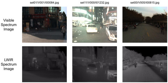
Figure 2.
Examples of visible–LWIR image pairs from KAIST dataset.
As clearly stated by the authors, the KAIST dataset is primarily aimed at accident avoidance, particularly in the context of pedestrian detection. This means that the images included are consecutive images focused on urban environments, all taken from a car perspective. This implies some limitations to the use case presented in this paper, which is discussed further in later sections.
KAIST Correction
The KAIST dataset is known to have calibrated pairs of images with the same field of view thanks to the beam splitter used. But, the images are not pixel-to-pixel matched due to the desynchronization of both cameras. Although a small gap between the capture of both images may seem to have a minor impact, this difference becomes significant with moving objects. This issue is particularly relevant for the KAIST dataset, as the images were captured from a moving vehicle.
The magnitude of this kind of distortion depends on both the speed of the vehicle and the relative distance between the objects and the camera. As anyone can imagine, the distortion varies from image to image, so there is no perfect solution to tackle this. For this specific dataset, the images were taken consecutively from a car. The desynchronization problem occurs because the LWIR image was taken before the visible-spectrum image, causing a small time lag of the visible images from their corresponding LWIR images. The transformation that could correct this distortion is a fraction of the transformation between that visible image and the previous image, as rresented in Figure 3, where T represents the affine transformation between consecutive visible images, while T’ represents the transformation between the visible image and the corresponding LWIR image.
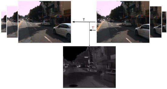
Figure 3.
Estimation of the transformation between LWIR and visible images based on consecutive visible images.
To compute this transformation, and taking advantage of the fact that the dataset contains consecutive images, the optical flow is computed for all the visible images in the dataset with respect to the previous image. Using this optical flow, which is based on matching key points between both images, the affine transformation between them can be computed, as expressed in Equation (1). Specifically, key points are first detected in the current visible image using the Shi–Tomasi corner detection algorithm [36]. These key points are then tracked in the previous visible image using the Lucas–Kanade optical flow method [37], and, finally, the transformation matrix is estimated using an approach based on RANSAC.
where T is the homogeneous affine transformation. With this transformation matrix, each pixel from Image 2 can be projected back to match Image 1, as in Equation (2), where are the coordinates in the visible image , and are the coordinates in the following visible image .
where elements a, b, c, and d in the matrix represent the rotation, scale, and shear transformations, while and represent the translation components of the affine transformation.
Given that the LWIR image is captured slightly earlier than , we assume that its corresponding transformation should be a scaled version of T. We define as
where S is a scaling function that adjusts T to compensate for the time difference between the capture of the LWIR and visible images. Applying to , we obtain the temporally corrected LWIR image with Equation (4):
As the distortion between images was more noticeable on the borders of the image, each image was slightly cropped. To maintain image size and future compatibility with additional data, the margins of the image were filled with a mosaic of the remaining parts of the image, following the mosaic approach of YOLOv8 data augmentation. Note that labeled objects in the remaining area were duplicated in the margins, leading to extra instances. The dataset labels were also refined to label specific pedestrians that were previously labeled under the general category of people. The resulting dataset is summarized in Table 3.

Table 3.
Summary of data from the corrected KAIST dataset used in tests: 80–20% split.
For reproducibility purposes, the source code of the image alignment correction tool (https://github.com/enheragu/multiespectral_correction, accessed on 26 February 2025) and the label review tool (https://github.com/enheragu/kaist-dataset-relabeling, accessed on 26 February 2025) are publicly available.
2.2.2. LLVIP Dataset
The LLVIP dataset [33] includes 16 k color–thermal image pairs (1080 × 720, 20 Hz) that were manually labeled (pedestrian). All images were taken in low-light conditions with a static camera at 26 different locations.
As shown in Table 4, the dataset is provided with a 80–20% split of the images, which were used in the experiments as such. The number of images is smaller than in the KAIST dataset but, in terms of pedestrian instances, is quite balanced. Note that, in this case, the number of images without detection targets is almost zero.

Table 4.
Summary of data from LLVIP dataset.
An example set of image pairs is shown in Figure 4. This dataset was acquired with a binocular camera from Hikvision. As a commercial camera, the images seem to have been preprocessed, and some equalization and autoexposure have been used. In this manner, the same temperature can be represented with different gray tones between images, leading to a better contrast but avoiding invariance to thermal conditions. In this case, the gray level on each part of the images depends not only on the body temperature but also on the thermal data and the general image brightness.
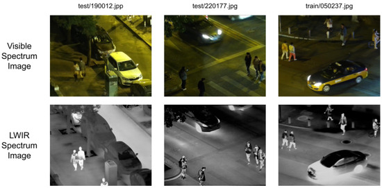
Figure 4.
Examples of visible–LWIR image pairs from LLVIP dataset.
2.3. Training Procedure
YOLOv8, as provided by the authors, can be fine-tuned with a custom dataset or it can be completely trained from scratch with custom data. The base model can be used out of the box as it was pretrained with the COCO dataset, as presented in [38], or fine-tuned with extra data. The COCO dataset is commonly used as a benchmark for detection-based models. This implies that the model was already trained with a huge source of information, which has a great impact on the performance obtained with each fusion algorithm, but it can also include extra noise that hinders the comparison between the fusion methods.
Since different architectures or fusion algorithms (middle or late fusion methods) cannot take advantage of this pretrained model, comparing the performance between them would include not only the differences between the algorithms to be compared (fusion) but also the ones from the pretrained model. This source of extra noise was isolated by training each model from scratch only with the selected dataset: KAIST. This way, different methods could be compared under the same conditions, whichwas not an easy task to find datasets with such requirements or to produce a new one.
To reduce potential sources of variability and to be able to compare the different methods and approaches, the same untrained model was used as the seed for all the tests. Following the same policy, and while it could impact performance and speed, the YOLOv8 algorithm was set to work in deterministic mode, as explained in [39].
Apart from controlling the external influence from other data, making use of the KAIST dataset alone also reduced the time needed for training and validating.
As may be obvious for the reader, to compete with other approaches, external datasets should be adapted to be included in the workflow so as to determine the best performance amongst them. In our case, the total number of images used during training was low, so the results in terms of detection are weak. However, this sufficed for the comparison between the different fusion methods, providing useful information about how to complete the dataset and in which direction to advance.
Finally, all the tests were performed with the same equipment, making use of an NVIDIA GPU, model GeForce RTX 4090 with 24 GB.
2.4. Evaluation and Metrics
To evaluate the performance of each approach, common metrics were used, such as precision, recall, and mean average precision (mAP). They are described below, and that is how they were used in this study. There are many ways to measure the performance of a deep learning implementation, each with its limitations and advantages. In order to provide a clear picture of all of them for the later discussion of the results, this section includes a description of all the metrics involved:
- Precision (P) reflects the proportion of true positives (TPs) in all positives detected by an algorithm, including both correctly detected instances (true positives) and instances incorrectly detected as positives (false positives, FPs). It assesses the capacity of the model to avoid false positives. Equation (5) summarizes this description.
- Recall (R) computes the proportion of true positives (TPs) in all real positives, including both instances correctly detected (true positives) and instances missed (false negatives, FNs). It measures the capacity of the system to detect all instances of a given class. Equation (6) shows the mathematical expression.
- F1-score is the harmonic mean (see Equation (7)) of both precision and recall, designed to provide a balanced metric between both, so that it allows evaluating model performance. Note that the results presented in the following section, provided with YOLOv8 for both precision and recall, were computed at the point at which F1 was maximized.
- Intersection over union (IoU) measures the overlap between the predicted box and the ground truth. It measures the capability of the algorithm to find instances of each class.
- Average-recision (AP) computes the area under the precision–recall curve. It gives a unique value that encodes both the precision and recall of the model.
- Mean average precision (mAP) expands the AP concept by averaging the mean precision between different classes. It is the more generic metric used to evaluate the performance of a model. Note that despite the fact that only one class was detected in the following tests (no average performed), the mAP is presented in Section 4 as it is the most commonly used metric. mAP is presented in two cases: mAP50, computed with an IoU of 0.5 to reflect the precision of the model considering easy detections; mAP50-95, which accumulates the average of the precision computed with different IoU thresholds that vary between 0.5 and 0.95.
- Log average miss rate (LAMR) is a popular metric in pedestrian detection tasks [30,34]. The miss rate (MR) reflects the percentage of pedestrians missed, as can be observed in Equation (8). False positives per image (FPPI) is a function of the confidence value (threshold in probability to accept or not a positive detection). As mAP makes use of the precision–recall curve, LAMR is computed based on the MR–FPPI plot. It averages the miss rate at nine different points along the FPPI axis () evenly spaced in log-space in the range of to (represented as f in the equation). Note that if there are no MR data in that part of the function, the highest existent FPPI is used as reference point. LAMR is computed as shown in Equation (9).
Note that each of the metrics are evaluated at different confidence values that include different variations in IoU thresholds. For each case, the measure is a function of this confidence, c (, , …).
3. Image Fusion Algorithms
The different multimodal systems, with regard to where the fusion is performed, can be split into three different approaches:
- Early fusion: Fusion occurs on raw data, before entering any detection algorithm. It has the advantage of allowing the usage of other unspefcific algorithms instead of having to develop a new approach for the specific data and use case.
- Middle fusion: Fusion occurs during the feature extraction of a network. All information sources are mixed to extract relevant features from the data.
- Late fusion: Fusion is performed in the decision layer, at the end of the network, when all the features are taken into account. In this way, specific feature extraction branches can be applied to each input and then merged once the relevant information is extracted. In this specific case, in the image detection domain, the fusion is performed in the dense layer where objects are detected and classified.
As explained by [40], early fusion methods have not been as thoroughly explored in the domain of multimodal fusion. It is not easy to find a fusion algorithm that can obtain relevant information between different sources of data (image, LIDAR, etc.). In the specific case of visible and thermal images, fusion is not as abstract, and it can be achieved without much difficulty. As already described by [40], we expect that these methods can be valuable and provide good results even when they are compared to more complex methods.
3.1. Early Fusion
In the early fusion approach, the visible and LWIR images are combined into a single three-channel image that is subsequently fed into a YOLO network for object detection (see Figure 5). The primary goal is to merge the information from all four spectral channels—three from the visible spectrum (red, green, and blue) and one from the thermal domain—into a format compatible with state-of-the-art convolutional neural networks such as YOLO, which are optimized for three-channel inputs.

Figure 5.
Architectural view of the methodology followed in this study with the early fusion approach, from the input images to the detected persons in the result.
To accomplish this, several static fusion methods have been proposed. Each method adjusts the relative weighting of the individual channels or directly manipulates the color components to compress the four-channel input (R, G, B, T) into three channels. The objective of these transformations is to minimize the loss of important target information during the channel reduction process.
It is important to note that these early fusion methods rely on the assumption that the scene captured in both the visible and thermal images is identical. The fixed transformation—termed the static fusion algorithm—applies the same fusion strategy uniformly across all images, without introducing any dataset-specific bias.
The following subsections detail four specific fusion strategies that have been developed to achieve this compression while retaining critical detection features.
3.1.1. RGBT
Trying to minimize information loss, both visible (RGB) and thermal (T) images are compressed into a three-channel image by multiplying the thermal channel with each of the other channels; each pixel value is then re-escalated to fit in the 8-bit image, as shown in Equation (10):
Then, the resulting image is based on each channel: , , and are merged back together as if they were RGB channels. This approach is similar to the one proposed in [16], but, instead of averaging the channels, they are multiplied. This way, different areas of the image for each of the R, G, and B channels are either highlighted or subdued based on the heat information from the thermal image.
3.1.2. HSVT
HSVT compresses both the visible (in HSV, hue–saturation–value, color encoding) and thermal image (T), combining the thermal channel with the intensity of the visible image. Next, the resulting channel is re-escalated back to fit in an 8-bit image. The transformation is performed as explained in the following equations:
Following Equation (11), the final image comprises channels , , and , which are merged back as if they were HSV channels. This transformation achieves a similar result as the previous one in Equation (10) in terms of highlighting visible-spectrum features by means of thermal information, but, in this case, the color information remains unmodified, and it is only the intensity channel that is changed.
3.1.3. VTHS
Depending on the illumination conditions under which a dataset was captured, color information may be less relevant compared to intensity (both from the visible- and thermal-spectrum images). If color information is not as relevant, a plausible fusion technique could be compressing it into only one of the three input channels. This way, the visible-spectrum image is split into HSV channels to keep the information from the brightness channel (V), compressing the hue (H) and saturation (S) channels into one and adding thermal information as the third channel. This way, both H and S are compressed into 4 bits each and merged into an 8-bit channel. In Equation (12), this transformation is represented with bit shifting notation (subindex 4 represents that a 4-bit representation from that channel is used):
Thus, the resulting image is composed of channels , , and , which are merged back together, keeping all the brightness information from both images unchanged and color information from the visible-spectrum images compressed.
3.1.4. VT
Continuing with the previous idea, if color is not relevant in the dataset, good results should be obtained by giving even more importance to brightness for both channels. This fusion method keeps the brightness from both images in the first and second channels, averaging both into the third one, as explained in Equation (13):
The resulting image is obtained by merging the three channels back together, now without any color information at all.
As a summary of this section, Figure 6 shows, in a false color representation, the result of each fusion method with a given image taken from the KAIST dataset. It is worth noting how some methods seem, at least visually, to highlight interesting parts of the scene as a result of the combination of the four channels. Figure 7 shows the same results based on an image from the LLVIP dataset. It is important to note that the results are slightly different because of not only different lightning conditions but also the range of data from different cameras (calibrated vs. autoexposure) since they may differ.

Figure 6.
Examples in false color representation of the result of each fusion method based on a KAIST dataset image. (a) HSVT fusion. (b) VT fusion. (c) RGBT fusion. (d) VTHS fusion.

Figure 7.
Examples in false color representation of the result of each fusion method based on an LLVIP dataset image. (a) HSVT fusion. (b) VT fusion. (c) RGBT fusion. (d) VTHS fusion.
3.2. Middle Fusion
In the middle fusion approach, the four channels are fed directly to a modified YOLOv8 network that is capable of handling the four channels and mixes them in the feature extraction stage. The data flow can be better observed in Figure 8.
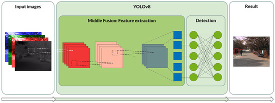
Figure 8.
Architectural view of the methodology followed with the middle fusion approach from the input images to the detected persons as the output.
Different variations in the YOLOv8 model were created to handle four raw input channels. Although the base model was previously modified, the experiments revealed a tendency to overfit. As a result, three different models are proposed, summarized in Table 5. The base YOLOv8 adapted for four-channel data was tested along with two different sizes with extra dropout layers, one after each C2f layer of the original YOLOv8 architecture.

Table 5.
Summary of size of each middle fusion variation.
The data loader was updated so that color data augmentation was applied to all four channels, making use of the HSV color space for visible images and a similar variation for the thermal channel.
3.3. Variations: Histogram Equalization
The methods presented in the previous subsections weight each channel to create the resulting fusion. These weighting operations are very sensitive to differences in the intensity levels of the channels being processed, meaning that large discrepancies or range restriction at these levels could significantly affect the final outcome.
Figure 9 shows a good example of the range restriction affecting LWIR images. As shown in the histogram in Figure 9a, it only has information in part of the X axis, leaving the rest of the histogram with zero values. This can be a problem when the information is merged with the other channels as the scale of the data differs between the images. An easy and promising solution to tackle this problem is histogram equalization. The left image in Figure 9a is an original image from the KAIST dataset [34] from the LWIR spectrum (in false color for a better appreciation of the equalization effects); its histogram clearly illustrates the range restriction issue already described. Figure 9b shows the result of histogram equalization, both the resulting image and its histogram. The range restriction problem was solved. However, image noise noticeably increased in the resulting image. The preferred solution, shown in Figure 9c, is applying an adaptive equalization: Contrast-Limited Adaptive Histogram Equalization (CLAHE). In this particular case, the image is split into 6 × 6 tiles to be locally equalized. Also, to avoid noise propagation, a contrast threshold is applied. The resulting image shows better contrast between objects of interest and background (these differences in the LWIR channel being represented in terms of temperature). Although part of the histogram is still unused (gray values higher than 200), the range restriction issue is notably improved, and the data are more evenly distributed throughout the whole range.
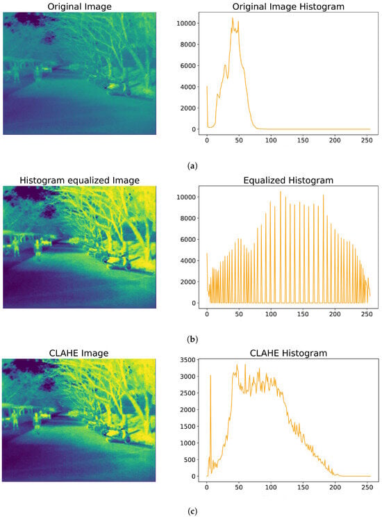
Figure 9.
Comparison of equalization techniques of LWIR histogram images from the KAIST dataset. (a) Original LWIR image with its histogram. (b) LWIR image and histogram processed with a standard equalization. (c) LWIR image and its histogram processed with CLAHE.
Following the same approach, RGB images can be equalized with the CLAHE method, applied to the luminance channel (Y) of the YCbCr color space of each image, based on [41]. It could provide better results than equalization on HSV or RGB color spaces. Usually, at night, some range restriction issues might appear due to the lack of light in the environment.
Note that YOLOv8 architecture normalizes all the input channels. Middle fusion algorithms should not suffer from the range restriction problem as the data are normalized independently. Tests with middle fusion algorithms were performed without any equalization.
4. Results
This section describes the results of this research. It is worth noting the impact of the previously described equalization method. The training results include the combination of the equalization of each image source and the fusion methods. Please also note that these fusion methods were proven to not compromise the real-time execution this use case requires, as shown in the following sections.
4.1. Preprocessing: Fusion Methods
All early fusion approaches have the disadvantage of increasing the processing time of the toolchain, since the information has to be fused before progressing to the deep model. Table 6 shows the mean time consumed by all fusion methods to obtain each of the processed images. Although the time consumed by the RGBT method is much longer than the rest of the methods, this is considered to be acceptable because, in this specific use case, it allows real-time processing at high speeds without delays or bottlenecks.

Table 6.
Summary of fusion time for each method.
4.2. Training Results
As previously described, there are multiple metrics that can be used for assessing the performance of a given dataset-algorithm pair. None of them provides a comprehensive view adaptable to all use cases. As a result, in this section, different metrics are analyzed for different purposes. While each plot is discussed individually, a summary of all metric results is presented in the tables at the end of each section. In all cases, apart from the four early fusion methods and the three middle fusion versions, the visible and LWIR spectra are included as references.
Due to the large number of possible combinations (each fusion method with or without equalization), the most intuitive starting point was to evaluate precision and recall, and evaluate how they affect the specific use case that this research focused on. Both metrics, as presented in the summary tables, were computed at the maximum F1 score and provide a robust comparison frame. Then, the precision recall curves were analyzed to see the evolution of both metrics at other working points apart from the maximum F1. Finally, these conclusions were compared to the rest of the metrics computed, which can be reviewed in the summary tables.
Note that the comparison includes not only the fusion method but also combinations in the equalization of the images. The same format is followed in all the images, with the tests tagged as follows:
- no_equalization: none of the images are equalized.
- rgb_equalization: only the visible image is equalized.
- rgb_th_equalization: both images, visible and thermal, are equalized.
- th_equalization: only the thermal image is equalized.
The following sections are focused on analyzing the training results with the described approach on both the LLVIP and KAIST datasets.
4.2.1. Training Results: LLVIP Dataset
The scenarios contemplated in this manuscript (e.g., SAR operations) require a higher recall so that no persons are left undetected. Increasing the recall is usually followed by a decrease in the precision metric. Although a higher recall is preferred, precision should not be too low. The idea is that a human operator could inspect the output of the algorithm to discard false positives while ensuring that false negatives are minimized. In terms of precision, in Figure 10, a good choice would be to take the LWIR images or the fusion provided by the CH4V3 method or the VT method. Note that thermal channel equalization seems to be relevant in terms of increasing the precision of the VT method and VTHS, whereas RGB equalization seems to provide worse results. In terms of recall, in Figure 11, the VT method clearly outperforms the rest, followed by VTHS and CH4V3. Again, thermal channel equalization seems to provide a relevant enhancement in the results.
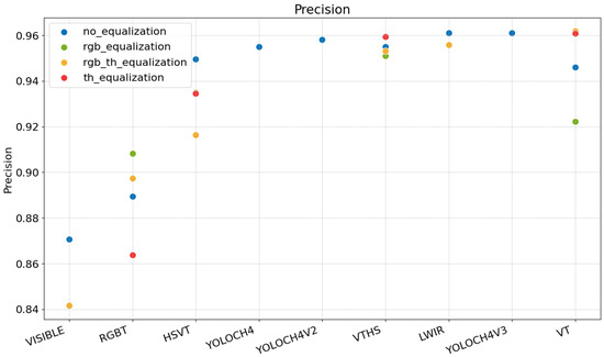
Figure 10.
Comparison of precision at maximum F1 between the different methods described based on training results with LLVIP dataset images.
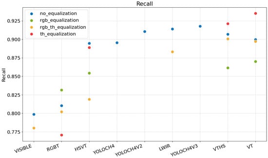
Figure 11.
Recall at maximum F1 comparison between the different methods described based on training results with LLVIP dataset images.
The precision–recall curve shown in Figure 12 also confirms the previous insights. The VT method provides better results compared with the rest (and compared with visible or LWIR images alone) in the whole plot.
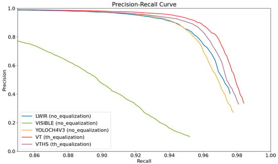
Figure 12.
Precision–recall curve at mAP0.5 for the selected methods with LLVIP dataset images.
All the metrics studied, presented in Table 7, validate these conclusions. mAP provides a good indicator of the general performance of a model, and it is really useful for comparing the performance of the different models and datasets; mAP50 is the standard metric, and mAP50-95 is the more restricting case. LAMR is commonly used in pedestrian detection because it provides an integrated measure of both the miss rate (related to recall) and false positives on images for different confidence thresholds (as shown in Equation (9)). The VT method provides better results in mAP50, miss rate, and LAMR. Focusing on the mAP50-95 metric, which provides a view of the algorithms’ performance under more severe conditions (higher confidence threshold for the predictions), the VTHS method (with thermal equalization) produces slightly better results.

Table 7.
Summary of training results on LLVIP dataset.
Note that the LLVIP dataset, as previously described, includes images in low-light conditions. The results with visible images only reflect these. Although LWIR images provide much better results, static early fusion methods prove to be valuable, even compared with the middle fusion methods tested in this study. As expected, in poor light conditions, where color information is not so relevant: better results are produced by a method that actually discards all color information, which is followed by the VTHS method that considerably reduces color information. Based on the results on the LLVIP dataset, it can be concluded that the fusion of visible and thermal data improves the results on the detection task with YOLOv8.
4.2.2. Training Results: KAIST Dataset Correction
To evaluate the performance of the previously described correction, a set of training tests were performed after and before correction was applied (Section 2.2.1). The RGBT and HSVT methods as well as the CH4 model were chosen for this comparison under equalization and non-equalization conditions with daylight images. Night images are less impacted, as LWIR information takes precedence over color data. The results of each training execution can be observed in Table 8. All results show an improvement in all the metrics with the corrected dataset with respect to the uncorrected version. Note that middle fusion approach seems to be more sensitive to the misalignment of the images. Also, as already stated, CH4 seems more prone to overfitting than the other methods, a situation highlighted by the desynchronization of the images. Although the correction algorithm could be refined, the results show that it already provides a good improvement. The experiments discussed in the following sections made use of the corrected version of the dataset only.

Table 8.
Comparison between results with and without correction of the dataset.
4.2.3. Training Results: KAIST Dataset
During daylight conditions, as expected, the LWIR data only produced very poor results both in precision, as presented in Figure 13, and recall, as shown in Figure 14. Having three channels with meaningful information is much more useful than only thermal information. Note that the dataset does not include challenging images such as those presented in Figure 1b or in Figure 1c, so both visible and LWIR results should be carefully inspected. Although using only LWIR did not produce valid outputs, once fused with the rest of the data, the precision improved, meaning that a notable false positive discrimination was achieved. In this sense, VTHS, which saves one whole channel for thermal data, produced the best performance in terms of precision, followed by the HSVT and RGBT methods, which enhanced the inputs from the RGB channels by adding thermal information. It is noticeable how thermal equalization only produced better results in the case of the VTHS fusion method, with worse results for the rest of the tests. The results on the KAIST dataset were not as consistent as those on the LLVIP dataset. With regard to recall, which is the ability of the solution to find all the instances in the image, the RGBT method proved to be the best, without the need for any equalization. It can be seen that although the thermal information provided a better detection of instances, the most instances detected occurred when the RGBT method was used, or when only visible data were used. The images in the dataset do not have much variance in color, as most come from a city environment with predominant dimmed and gray tones. This fact suggests that HSVT could provide better results in other scenarios. Note that the HSVT method already provides good results in terms of precision, so it should be a good candidate in daylight conditions with more varied images. The precision–recall curves below provide a clearer assessment of which method should be preferred.
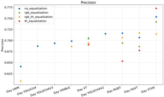
Figure 13.
Comparison of precision at maximum F1 between different methods described based on training results with daylight images from KAIST dataset.
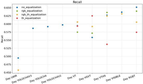
Figure 14.
Comparison of recall at maximum F1 between the different methods described based on training results with daylight images from KAIST dataset.
In the case of the night condition images presented in Figure 15 and Figure 16, the results slightly changed.
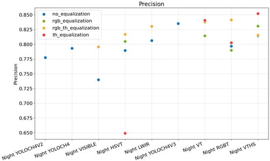
Figure 15.
Comparison of precision at maximum F1 between different methods described based on training results using night condition images from KAIST dataset.
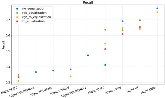
Figure 16.
Comparison of recall at maximum F1 between different methods described based on training results using night condition images from KAIST dataset.
In this scenario, the color information is poorer, and the LWIR channel has a larger influence. In terms of the precision metric, VTHS with the equalization of the thermal channel provides the best results, followed by RGBT, which equalizes both the thermal and RGB channels (separate equalization of RGB or thermal channel seems to provide similar results to no equalization). The absence of light in certain areas of the images (despite the presence of artificial lighting from paths and roads) may have caused effects similar to those previously described as caused by range restriction. Thus, equalization becomes increasingly important, as observed in the cases of the RGBT, VTHS, and VT methods.
In terms of recall, RGBT produced the worst results, as it was likely to find the most obvious instances without many false positives and, at the same time, left many instances undetected. The best recall was achieved when the LWIR channel was used alone. Again, no challenging data are available in the dataset, so there were not many situations where LWIR could benefit from other fusions, which is something that would not happen with more difficult data. Color information is not very important, as demonstrated by the results of the VT fusion, followed by VTHS. Both take the intensity information of the RGB channels, disregarding color data.
To better assess these results, the precision–recall curves can be reviewed. In this case, Figure 17 shows the precision–recall curve for a subset of the proposed fusions in daylight conditions, while Figure 18 shows the analogue representation using night condition images. For easier interpretation, only a subset of the methods and conditions are presented, and the plot focuses on a recall range that is relevant for the analysis.
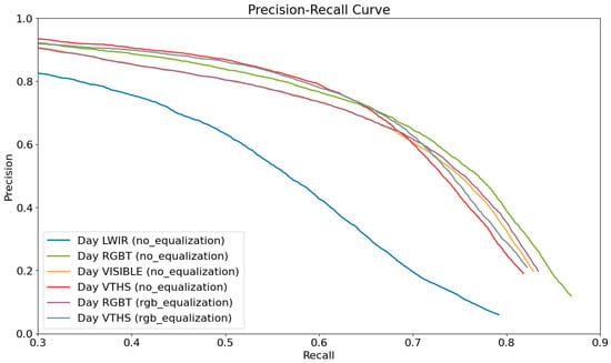
Figure 17.
Precision–recall curve (mAP0.5) for most promising methods under daylight conditions.
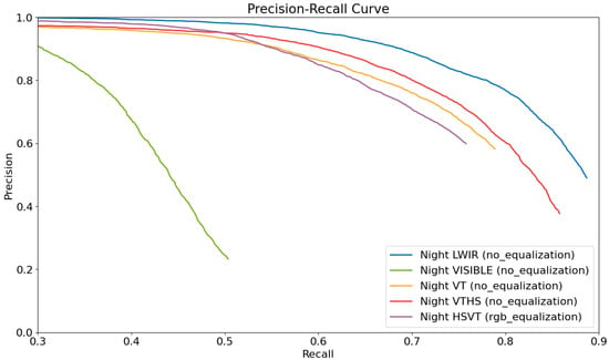
Figure 18.
Precision–recall curve (mAP0.5) for most promising methods under night conditions.
With regard to daylight conditions, VTHS seems to provide quite good results in terms of precision, but these results degrade when recall increases. At higher recalls, RGBT is able to maintain good precision. All of them produce better results than visible or LWIR data alone, which are provided as a reference. With this information and on the KAIST dataset, RGBT proves to be the best approach under daylight conditions. Under night conditions, LWIR alone clearly stands out, followed by VTHS with no equalization. With this dataset, LWIR should be the preferred option, although, as already explained, with more challenging datasets, VTHS could be more suitable.
Focusing on the data in Table 9, in terms of both recall and mAP50, RGBT without equalization proves to be the best. These conclusions align with what was previously stated regarding Figure 14 and Figure 17. For a more restrictive metric, mAP50-95,the VTHS method is the one that provides better results, which aligns with the conclusions extracted from Figure 13. Once again, for these methods and conditions, equalization does not contribute significantly to producing better detection results. When compared, the metrics support with the conclusion of using the RGBT fusion method for better detection under daylight conditions.

Table 9.
Summary of results of different tests under day conditions for each fusion algorithm on KAIST dataset images.
Under night conditions, the conclusions are not as clear as before. Table 10 shows a summary of all the tests with their associated performance metrics. In terms of recall, miss rat, and mAP50, LWIR images alone without equalization are the ones that stand out, as consistently observed in Figure 16 and in Figure 18. In a more restrictive scenario, based on mAP50-95, VT without equalization provides better results. Based on the LAMR metric, VTHS is preferred, which aligns with the conclusions if more importance is given to precision, as shown in Figure 16.

Table 10.
Summary of results of different tests under night conditions for each fusion algorithm on KAIST dataset images.
The middle fusion algorithms do not provide good enough results. Although a larger network and dropout inclusion should lead to better results, these algorithms are less precise than simpler fusion methods. In all cases, overfitting is a problem for the different versions of the model. Note that the split of the train and test images from the dataset was made so that the images were from quite different scenarios, which would have made the models vulnerable to overfitting. In other cases, this overfitting might be unnoticed, but the generalization issue it creates would still be present.
4.2.4. Training Results: Conclusions
LLVIP and KAIST have different characteristics that should be taken into account when evaluating the results. As already described, LLVIP only contains low-light condition images that were acquired in similar conditions (all urban areas). As the images were captured in urban areas, the illumination is not as good as in daylight, but the view is clear in the visible-spectrum images. The LLVIP images primarily include close-up shots with minimal background, something that also benefits more uniform illumination. On the other hand, the KAIST dataset includes both day and night condition images, taken in four different scenarios. Some of the scenarios also have good illumination under night conditions. As the images were acquired from a vehicle, the perspective includes more background information, persons that vary in size, and less uniform illumination. The split between the test and train datasets reflects the difference in scenarios, making KAIST a better option for evaluating the generalization capabilities of the system. Finally, LLVIP is well aligned and synchronized, making the results in terms of fusion more robust than with the KAIST dataset, which is desynchronized.
Even with these limitations, the conclusions are consistent for both datasets. The LLVIP data shows better performance in VT and VTHS, which agrees with the night condition results from KAIST. In the KAIST scenario, LWIR produces better results than the other methods, probably due to the misalignment of the images not being sufficiently corrected.
In both cases, simple middle fusion algorithms are not able to provide better results than the methods studied in these experiments. Other methods should be studied with other changes to the YOLOv8 architecture or with other architectures.
5. Conclusions
This research focused on a set of fusion methods to combine visible and LWIR images to enhance performance on a detection task under different lightning conditions. The importance of the quality of the data was also examined, along with its format and usage (train/test split) as it is of major importance to be able to obtain good results as well as generalization capabilities while knowing the limitations of the selected approach.
Rigorous experimental controls were implemented and explained in this paper. We found that such control is of extreme importance to ensure the validity and repeatability of the tests and the conclusions drawn from them. Excluding pretrained models based on COCO was important to be able to compare early fusions methods and middle fusion methods, even at the cost of impacting the obtained results.
We consequently defined an experimental setup to control that potential bias and to establish a common benchmark for all the fusion approaches that were compared. Taking this into consideration, these experiments excluded other sources of bias, and we trained from zero the YOLO detection stack with only the KAIST or LLVIP dataset. This way, four different RGB-T early fusion methods with and without equalization, along with three middle fusion versions, were compared under the same conditions.
The presented results proved that splitting the problem into day and night conditions was a good decision. Environments such as SAR operations or surveillance need a robust solution in terms of their sensitivity to false negatives. Thermal information mixed with visible-spectrum images leads to better detection results. As supported by the tests on the KAIST and LLVIP datasets, our findings demonstrate that under low-light conditions, both the VT and VTHS methods provide promising results. This means that color information is not as useful as brightness and thermal data. During daylight, color information becomes more relevant, with RGBT being the method that provides better results. Even though the processing time is negligible for all the methods used, both VTHS and VT stand out as the most efficient.
Evaluation metrics are a key point in the field of machine learning not only during training or validation but also when sharing results and comparing methods with other state-of-the-art approaches. Although standardization is needed to compare the results between different works, it is important to remember that, for different specific use cases, these metrics alone might not be the best approach. Having a bigger picture including other metrics, even if they seem redundant, can provide a better understanding of the solutions being compared and lead to better decisions. In this specific case, recall proved to be a paramount metric in choosing a robust method.
It is also important to remark on the limitations of this paper. Despite the fact that the KAIST and LLVIP datasets proved to be valuable in reaching robust results, both have constraints that should be taken into account. All the fusion methods described suffer from misalignment between images. Future research should apply a better correction approach on to the KAIST dataset. A new dataset should include more challenging information, as presented in the Introduction, which neither KAIST nor LLVIP include. Although LLVIP includes quality data, it has minimal variety in terms of background or smaller objects instances, which would be more representative of the use case presented in this manuscript.
We conclude that the fusion of extra thermal data is relevant and beneficial under both daylight and night conditions. Simple methods can be very powerful in terms of performance but also robustness in regard to image distortion or overfitting. Future research could include comparisons with other early, middle, and late fusion methods. The analysis revealed a critical gap in existing datasets, highlighting the need for a novel, more comprehensive dataset to address the limitations of the current resources.
Author Contributions
Conceptualization: E.H.-A., D.V. and A.G.; methodology: E.H.-A., D.V. and A.G.; software: E.H.-A., J.J.C. and L.M.J.; formal analysis and investigation: E.H.-A., J.J.C. and L.M.J.; writing—original draft preparation: E.H.-A., D.V. and A.G.; writing—review and editing: E.H.-A., J.J.C., L.M.J., D.V. and A.G.; supervision: D.V. and A.G.; funding acquisition and project administration: A.G. All authors have read and agreed to the published version of this manuscript.
Funding
This research work is part of project TED2021-130901B-I00 funded by MICIU/AEI/10.13039/501100011033 and by the European Union NextGenerationEU/PRTR. It was also part of project PID2023-149575OB-I00 funded by MICIU/AEI/10.13039/501100011033 and by FEDER, UE.
Data Availability Statement
No new data were generated during this study. Please refer to [34] to obtain the KAIST dataset or more information about it.
Conflicts of Interest
The authors declare no conflicts of interest.
Abbreviations
The following abbreviations are used in this manuscript:
| AP | Average Precision |
| CNN | Convolutional Neural Network |
| FPPI | False Positives per Image |
| IoU | Intersection over Union |
| LWIR | Long-Wavelength Infrared |
| LAMR | Log Average Miss Rate |
| mAP | Mean Average Precision |
| MR | Miss Rate |
| NIR | Near Infrared |
| SWIR | Short-Wavelength Infrared |
| SAR | Search and Rescue |
| SOTA | State of the Art |
| UAV | Unmanned Aerial Vehicle |
References
- Girshick, R.B.; Donahue, J.; Darrell, T.; Malik, J. Rich feature hierarchies for accurate object detection and semantic segmentation. arXiv 2013, arXiv:1311.2524. [Google Scholar]
- Girshick, R.B. Fast R-CNN. arXiv 2015, arXiv:1504.08083. [Google Scholar]
- Ren, S.; He, K.; Girshick, R.B.; Sun, J. Faster R-CNN: Towards Real-Time Object Detection with Region Proposal Networks. arXiv 2015, arXiv:1506.01497. [Google Scholar] [CrossRef] [PubMed]
- Redmon, J.; Divvala, S.K.; Girshick, R.B.; Farhadi, A. You Only Look Once: Unified, Real-Time Object Detection. arXiv 2015, arXiv:1506.02640. [Google Scholar]
- Vaswani, A.; Shazeer, N.; Parmar, N.; Uszkoreit, J.; Jones, L.; Gomez, A.N.; Kaiser, L.; Polosukhin, I. Attention Is All You Need. arXiv 2017, arXiv:1706.03762. [Google Scholar]
- Carion, N.; Massa, F.; Synnaeve, G.; Usunier, N.; Kirillov, A.; Zagoruyko, S. End-to-End Object Detection with Transformers; Springer: Cham, Switzerland, 2020; pp. 213–229. [Google Scholar] [CrossRef]
- Grujić, K. A Review of Thermal Spectral Imaging Methods for Monitoring High-Temperature Molten Material Streams. Sensors 2023, 23, 1130. [Google Scholar] [CrossRef]
- Usamentiaga, R.; Venegas, P.; Guerediaga, J.; Vega, L.; Molleda, J.; Bulnes, F.G. Infrared Thermography for Temperature Measurement and Non-Destructive Testing. Sensors 2014, 14, 12305–12348. [Google Scholar] [CrossRef]
- Švantner, M.; Lang, V.; Skála, J.; Kohlschütter, T.; Honner, M.; Muzika, L.; Kosová, E. Statistical Study on Human Temperature Measurement by Infrared Thermography. Sensors 2022, 22, 8395. [Google Scholar] [CrossRef] [PubMed]
- Johnson, W.R.; Hook, S.J.; Mouroulis, P.; Wilson, D.W.; Gunapala, S.D.; Realmuto, V.; Lamborn, A.; Paine, C.; Mumolo, J.M.; Eng, B.T. HyTES: Thermal imaging spectrometer development. In Proceedings of the 2011 Aerospace Conference, Big Sky, MT, USA, 5–12 March 2011; pp. 1–8. [Google Scholar] [CrossRef]
- Speakman, J.R.; Ward, S. Infrared thermography: Principles and applications. Zoology-Jena- 1998, 101, 224–232. [Google Scholar]
- Ibarra-Castanedo, C.; Maldague, X.P.V. Infrared Thermography. In Handbook of Technical Diagnostics: Fundamentals and Application to Structures and Systems; Czichos, H., Ed.; Springer: Berlin/Heidelberg, Germany, 2013; pp. 175–220. [Google Scholar] [CrossRef]
- Ivašić-Kos, M.; Krišto, M.; Pobar, M. Human Detection in Thermal Imaging Using YOLO. In Proceedings of the 2019 5th International Conference on Computer and Technology Applications, Istanbul, Turkey, 16–17 April 2019; ICCTA ’19. pp. 20–24. [Google Scholar] [CrossRef]
- Kalita, R.; Talukdar, A.K.; Kumar Sarma, K. Real-Time Human Detection with Thermal Camera Feed using YOLOv3. In Proceedings of the 2020 IEEE 17th India Council International Conference (INDICON), New Delhi, India, 10–13 December 2020; pp. 1–5. [Google Scholar] [CrossRef]
- Redmon, J.; Farhadi, A. YOLOv3: An Incremental Improvement. arXiv 2018, arXiv:1804.02767. [Google Scholar]
- Vandersteegen, M.; Van Beeck, K.; Goedemé, T. Real-Time Multispectral Pedestrian Detection with a Single-Pass Deep Neural Network. In Proceedings of the Image Analysis and Recognition; Campilho, A., Karray, F., ter Haar Romeny, B., Eds.; Springer: Cham, Switzerland, 2018; pp. 419–426. [Google Scholar]
- Mao, S.; Duan, J.; Zhang, Z.; Zhang, Z. Visible and Infrared Image Fusion via Superpixel Segmentation and Salient Region Detection. In Proceedings of the 2021 36th Youth Academic Annual Conference of Chinese Association of Automation (YAC), Nanchang, China, 28–30 May 2021; pp. 643–648. [Google Scholar] [CrossRef]
- Chipman, L.; Orr, T.; Graham, L. Wavelets and image fusion. In Proceedings of the International Conference on Image Processing, Washington, DC, USA, 23–26 October 1995; Volume 3, pp. 248–251. [Google Scholar] [CrossRef]
- Su, H.; Jung, C. Multi-Spectral Fusion and Denoising of RGB and NIR Images Using Multi-Scale Wavelet Analysis. In Proceedings of the 2018 24th International Conference on Pattern Recognition (ICPR), Beijing, China, 20–24 August 2018; pp. 1779–1784. [Google Scholar] [CrossRef]
- Oishi, Y.; Yoshida, N.; Oguma, H. Detecting Moving Wildlife Using the Time Difference between Two Thermal Airborne Images. Remote Sens. 2024, 16, 1439. [Google Scholar] [CrossRef]
- Xiang, J.; Gou, S.; Li, R.; Zheng, Z. RGB-Thermal based Pedestrian Detection with Single-Modal Augmentation and ROI Pooling Multiscale Fusion. In Proceedings of the IGARSS 2022—2022 IEEE International Geoscience and Remote Sensing Symposium, Kuala Lumpur, Malaysia, 17–22 July 2022; pp. 3532–3535. [Google Scholar] [CrossRef]
- Zhou, H.; Sun, M.; Ren, X.; Wang, X. Visible-Thermal Image Object Detection via the Combination of Illumination Conditions and Temperature Information. Remote Sens. 2021, 13, 3656. [Google Scholar] [CrossRef]
- Zhang, Y.; Yin, Y.; Shao, Z. An Enhanced Target Detection Algorithm for Maritime Search and Rescue Based on Aerial Images. Remote Sens. 2023, 15, 4818. [Google Scholar] [CrossRef]
- Tian, W.; Deng, Z.; Yin, D.; Zheng, Z.; Huang, Y.; Bi, X. 3D Pedestrian Detection in Farmland by Monocular RGB Image and Far-Infrared Sensing. Remote Sens. 2021, 13, 2896. [Google Scholar] [CrossRef]
- Niedzielski, T.; Jurecka, M.; Miziński, B.; Pawul, W.; Motyl, T. First Successful Rescue of a Lost Person Using the Human Detection System: A Case Study from Beskid Niski (SE Poland). Remote Sens. 2021, 13, 4903. [Google Scholar] [CrossRef]
- Gotovac, S.; Zelenika, D.; Marušić, Z.; Božić-Štulić, D. Visual-Based Person Detection for Search-and-Rescue with UAS: Humans vs. Machine Learning Algorithm. Remote Sens. 2020, 12, 3295. [Google Scholar] [CrossRef]
- Zhang, H.; Wu, C.; Zhang, Z.; Zhu, Y.; Lin, H.; Zhang, Z.; Sun, Y.; He, T.; Mueller, J.; Manmatha, R.; et al. ResNeSt: Split-Attention Networks. In Proceedings of the 2022 IEEE/CVF Conference on Computer Vision and Pattern Recognition Workshops (CVPRW), New Orleans, LA, USA, 19–20 June 2022; pp. 2735–2745. [Google Scholar] [CrossRef]
- Zong, Z.; Song, G.; Liu, Y. Detrs with collaborative hybrid assignments training. In Proceedings of the IEEE/CVF International Conference on Computer Vision, Paris, France, 1–6 October 2023; pp. 6748–6758. [Google Scholar]
- Jocher, G.; Chaurasia, A.; Qiu, J. YOLOv8 by Ultralytics; Ultralytics YOLO (Version 8.0.0) [Computer Software]. 2023. Available online: https://github.com/ultralytics/ultralytics (accessed on 20 December 2024).
- Braun, M.; Krebs, S.; Flohr, F.B.; Gavrila, D.M. EuroCity Persons: A Novel Benchmark for Person Detection in Traffic Scenes. IEEE Trans. Pattern Anal. Mach. Intell. 2019, 41, 1844–1861. [Google Scholar] [CrossRef] [PubMed]
- FLIR. FREE Teledyne FLIR Thermal Dataset for Algorithm Training. 2023. Available online: https://www.flir.com/oem/adas/adas-dataset-form/ (accessed on 20 December 2024).
- Zhang, L.; Zhu, X.; Chen, X.; Yang, X.; Lei, Z.; Liu, Z. Weakly Aligned Cross-Modal Learning for Multispectral Pedestrian Detection. In Proceedings of the 2019 IEEE/CVF International Conference on Computer Vision (ICCV), Seoul, Republic of Korea, 27 October–2 November 2019; pp. 5126–5136. [Google Scholar] [CrossRef]
- Jia, X.; Zhu, C.; Li, M.; Tang, W.; Zhou, W. LLVIP: A visible-infrared paired dataset for low-light vision. In Proceedings of the IEEE/CVF International Conference on Computer Vision, Montreal, BC, Canada, 11–17 October 2021; pp. 3496–3504. [Google Scholar]
- Hwang, S.; Park, J.; Kim, N.; Choi, Y.; Kweon, I.S. Multispectral pedestrian detection: Benchmark dataset and baseline. In Proceedings of the 2015 IEEE Conference on Computer Vision and Pattern Recognition (CVPR), Boston, MA, USA, 7–12 June 2015; pp. 1037–1045. [Google Scholar] [CrossRef]
- Karasawa, T.; Watanabe, K.; Ha, Q.; Tejero-De-Pablos, A.; Yoshitaka, U.; Harada, T. Multispectral Object Detection for Autonomous Vehicles. In Proceedings of the 25th Annual ACM International Conference on Multimedia, Mountain View, CA, USA, 23–27 October 2017. [Google Scholar]
- Shi, J.; Tomasi. Good features to track. In Proceedings of the 1994 Proceedings of IEEE Conference on Computer Vision and Pattern Recognition, Seattle, WA, USA, 21–23 June 1994; pp. 593–600. [Google Scholar] [CrossRef]
- Lucas, B.D.; Kanade, T. An Iterative Image Registration Technique with an Application to Stereo Vision. In Proceedings of the 7th International Joint Conference on Artificial Intelligence, Vancouver, BC, Canada, 24–28 August 1981; pp. 674–679. [Google Scholar]
- Lin, T.; Maire, M.; Belongie, S.J.; Bourdev, L.D.; Girshick, R.B.; Hays, J.; Perona, P.; Ramanan, D.; Dollár, P.; Zitnick, C.L. Microsoft COCO: Common Objects in Context. arXiv 2014, arXiv:1405.0312. [Google Scholar]
- Jocher, G.; Qiu, J. Ultralytics YOLOv8 Documentation, Software Documentation; Ultralitics: Frederick, MD, USA, 2024.
- Boulahia, S.Y.; Amamra, A.; Madi, M.R.; Daikh, S. Early, intermediate and late fusion strategies for robust deep learning-based multimodal action recognition. Mach. Vis. Appl. 2021, 32, 121. [Google Scholar] [CrossRef]
- Mathur, P.; Soni, B. Exploring Color Models for Enhancement of Underwater Image. In Proceedings of the Data Driven Approach Towards Disruptive Technologies; Singh, T.P., Tomar, R., Choudhury, T., Perumal, T., Mahdi, H.F., Eds.; Springer: Singapore, 2021; pp. 325–336. [Google Scholar]
Disclaimer/Publisher’s Note: The statements, opinions and data contained in all publications are solely those of the individual author(s) and contributor(s) and not of MDPI and/or the editor(s). MDPI and/or the editor(s) disclaim responsibility for any injury to people or property resulting from any ideas, methods, instructions or products referred to in the content. |
© 2025 by the authors. Licensee MDPI, Basel, Switzerland. This article is an open access article distributed under the terms and conditions of the Creative Commons Attribution (CC BY) license (https://creativecommons.org/licenses/by/4.0/).