Forest Aboveground Biomass Estimation in Küre Mountains National Park Using Multifrequency SAR and Multispectral Optical Data with Machine-Learning Regression Models

Abstract

Aboveground biomass (AGB) is crucial in forest ecosystems and is intricately linked to the carbon cycle and global climate change dynamics. This study investigates the efficacy of synthetic aperture radar (SAR) data from the X, C, and L bands, combined with Sentinel-2 optical imagery, vegetation indices, gray-level co-occurrence matrix (GLCM) texture metrics, and topographical variables in estimating AGB in the Küre Mountains National Park, Türkiye. Four machine-learning regression models were employed: partial least squares (PLS), least absolute shrinkage and selection operator (LASSO), multivariate linear, and ridge regression. Among these, the PLS regression (PLSR) model demonstrated the highest accuracy in AGB estimation, achieving an R² of 0.74, a mean absolute error (MAE) of 28.22 t/ha, and a root mean square error (RMSE) of 30.77 t/ha. An analysis across twelve models revealed that integrating ALOS-2 PALSAR-2 and SAOCOM L-band satellite data, particularly the SAOCOM HV and ALOS-2 PALSAR-2 HH polarizations with optical imagery, significantly enhances the precision and reliability of AGB estimations.

1. Introduction

Forests are vital assets for societies worldwide, gaining ever more significance for sustaining life. Forests constitute the important sinks in terrestrial ecosystems that can reduce atmospheric emissions with the carbon they simultaneously store in the vegetative mass and the soil. The transformation of carbon into living biomass occurs through photosynthesis, and its conversion back to the atmosphere as CO₂ is facilitated by subsequent chemical reactions [1]. Therefore, accurate inventory, monitoring, and estimating forest biomass at regional and global scales are critical for reducing carbon emissions and increasing carbon sink areas in combating climate change [2,3].

Forest management relies heavily on assessing forest aboveground biomass (AGB), which is an important indicator of forests’ carbon storage capacity. Its estimation is essential for understanding and managing forest resources that are critical to carbon fluxes [4,5]. Both destructive and non-destructive methods are utilized to determine biomass, encompassing trees’ dry weight, significant AGB, belowground biomass, dead wood, litter, and soil organic matter. While destructive-method measurements offer the most precision in estimating AGB, they are also costly, labor-intensive, and time-consuming [6]. Recent advancements in satellite remote sensing have significantly improved the assessment of forest biomass and carbon stocks. Data from passive (optical) and active (e.g., synthetic aperture radar (SAR) and light detection and ranging (LiDAR) offer powerful tools for evaluating forest ecosystem structure, composition, and AGB [7]. Estimating AGB using optical sensors, which establish correlations between spectral responses and the ground data acquired from field plots, proves highly effective for estimating foliar biomass components [8,9]. Conversely, SAR systems, operable in all weather conditions, penetrate forest canopies to interact with woody stems and other components of trees [10,11]. The sensitivity of SAR to AGB varies with wavelength: longer wavelengths increase scattering saturation thresholds and strengthen the correlation between radar backscatter and biomass, leading prior studies to favor long-wavelength bands for biomass estimation [12,13,14,15]. A comparative analysis of SAR satellites operating at different frequency bands—the L-band (~1.2 GHz), C-band (~5.4 GHz), and X-band (~9.6 GHz)—highlights their varying effectiveness in AGB retrieval, primarily governed by frequency-dependent penetration capabilities [16]. L-band sensors exhibit superior penetration, effectively capturing structural information from trunks and branches in high-biomass ecosystems, such as tropical forests, where saturation occurs beyond 150 t/ha [12]. Conversely, the C-band demonstrates moderate penetration, primarily interacting with the canopy layer, making it suitable for intermediate biomass ranges (50–100 t/ha). In contrast, the X-band, characterized by dominant surface scattering, is most effective in low-biomass environments (<50 t/ha) [13]. Various studies have underscored the importance of SAR backscatter in estimating forest biomass across different frequency bands and have shed light on the relationship between polarimetric SAR backscatter. Sandberg et al. [16] found that the HV polarization of the L-band SAR outperformed HH polarization. Furthermore, Symeonakis et al. [17] highlighted that HV polarization shows greater sensitivity in dry weather conditions compared to HH or HV in rainy weather. Bhavsar et al. [18] focused on evaluating AGB in the tropical forests of Tripura, India, using SAR data from two distinct sensors. Their findings revealed improvements in HV polarization from both sensor platforms.

Recent studies have demonstrated that integrating SAR and optical data is sufficient for accurately estimating AGB using various sensor combinations that have been effectively utilized to improve the reliability of AGB estimations, such as TerraSAR-X (TSX) and Sentinel-2 (S2) [19], Sentinel-1 (S1) and S2 [20,21,22,23,24,25,26], The Advanced Land Observing Satellite-2 Phased Array Type L-band Synthetic Aperture Radar-2 (ALOS-2 PALSAR-2) and S2 [27,28], S1, ALOS-2 PALSAR-2, and S2 [29,30].

The selection of an appropriate algorithm for accurately estimating AGB is vital. In previous studies, linear regression (LR) has been the most widely adopted parametric method for AGB estimation [31]. The ridge regression model, which has been applied to resolve the instability or inactivation of least squares estimation in the multivariate linear regression (MLR) model, was developed by Hoerl and Kennard [32]. The partial least squared regression (PLSR) combines the essential functions of MLR, principal component analysis, and canonical correlation analysis and was developed by Wold et al. [33], and least absolute shrinkage and selection operator (LASSO) regression, an LR analysis method utilized for variable selection and regularization, is used in many forest studies [34,35,36,37]. Non-parametric techniques, including machine-learning (ML) methods such as support vector regressor (SVR), decision trees, K-nearest neighbor (KNN), artificial neural network (ANN), and convolutional neural networks (CNN), have also been utilized for remote-sensing estimation of forest AGB [38,39,40]. Ensemble learning, which involves constructing and combining multiple learners, has gained significant attention recently. It can incorporate decision trees and neural networks individually or in combination, primarily falling into Bagging and Boosting algorithms. Bagging enhances model generalization by reducing variance, with random forest (RF) being a well-known technique within the Bagging framework. This method constructs an ensemble of trees, each generated from a bootstrap sample of the training data [41]. Conversely, boosting employs ML algorithms to transform weak learners into strong learners, enhancing the model’s accuracy. Boosting encompasses various techniques such as adaptive boosting (AdaBoost), gradient-boosting decision tree (GBDT), extreme gradient boosting (XGBoost), light gradient-boosting machine (LightGBM), and categorical boosting (CatBoost) [20,42,43,44,45,46]. To address the inherent complexities of this study, we strategically selected four ML regression methods—LASSO regression, Ridge regression, MLR, and PLSR—which were driven by the need to capture the diverse strengths of each approach in handling the complexities of AGB estimation. LASSO regression is widely recognized in the literature for its ability to perform variable selection and model simplification, while Ridge regression addresses multicollinearity issues [32]. MLR is a foundational method for modeling linear relationships between dependent and independent variables, making it a standard choice in many applications [31]. Conversely, PLSR is favored for its capacity to handle high-dimensional, multicollinear data through dimensionality reduction. As intended, this strategic choice of models leverages their complementary strengths to address the multifaceted challenges of AGB estimation, aiming to identify the most suitable solution tailored to the dataset’s characteristics and the nature of the prediction problem [33].

This study pioneers the integration of L-band Satélite Argentino de Observación Con Microondas (SAOCOM), ALOS-2 PALSAR-2, TerraSAR-X (X-band), and Sentinel-1A (C-band) SAR imagery, Sentinel-2A multispectral imagery, vegetation indices, texture measures, and topographical data—a combination not comprehensively explored in prior AGB estimation research. This novel synthesis of advanced SAR, optical imagery, and field-based observations provides a more robust and precise framework for AGB estimation. Furthermore, by employing four ML regression methods—LASSO, Ridge, MLR, and PLSR—alongside three feature selection techniques, our approach leverages their complementary strengths to address the multidimensional challenges of AGB prediction, moving beyond the single-model frameworks prevalent in the recent literature. Notably, this study is the first to apply such an extensive satellite data framework to Küre Mountains National Park (KMNP), Türkiye, targeting two distinct species and offering fresh insights into region and species-specific AGB dynamics. Ultimately, this work advances the field by enhancing our understanding of multifrequency SAR and multispectral optical data applications, benefiting researchers, policymakers, and the scientific community in assessing forest impacts on ecosystems.

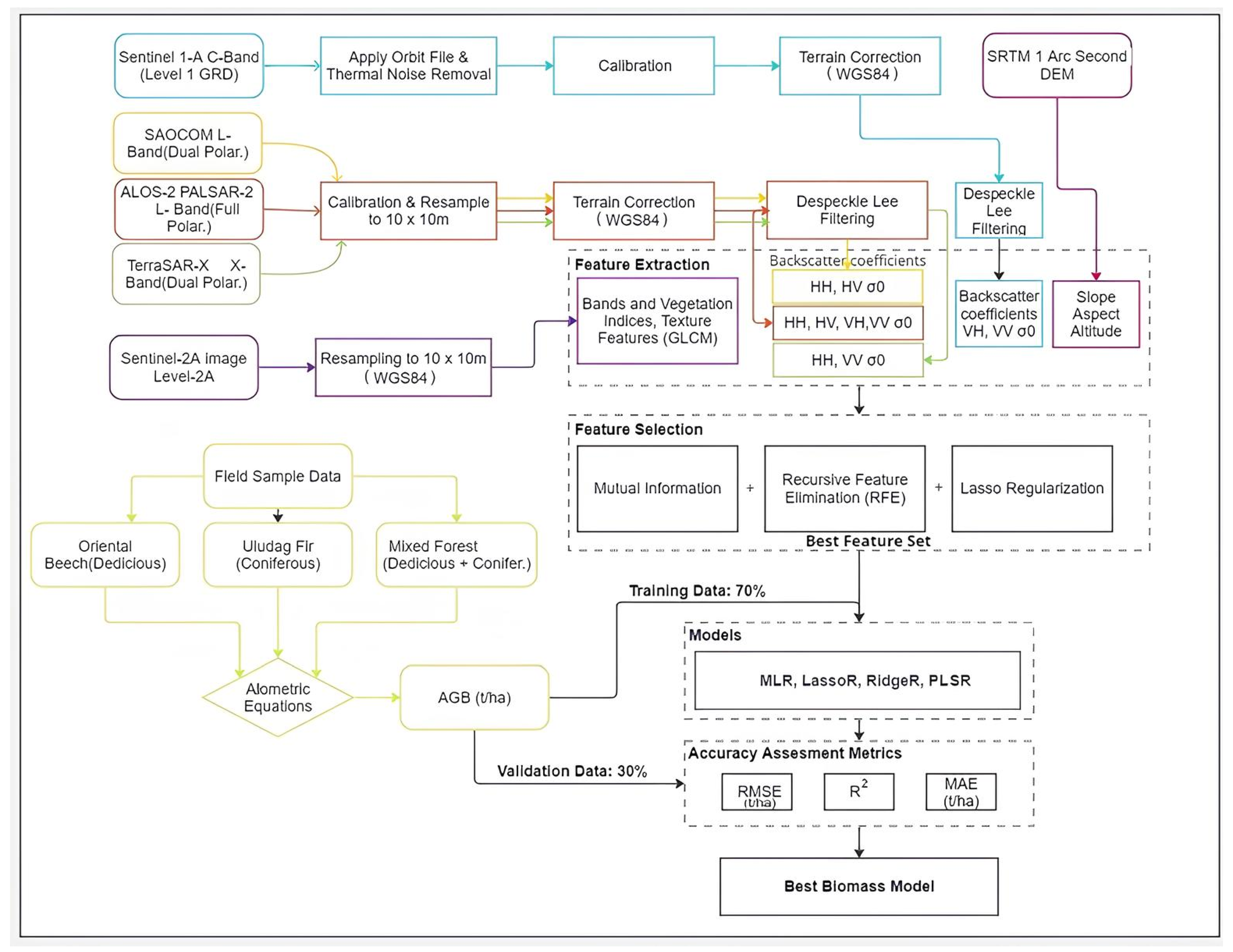
2. Materials and Methods

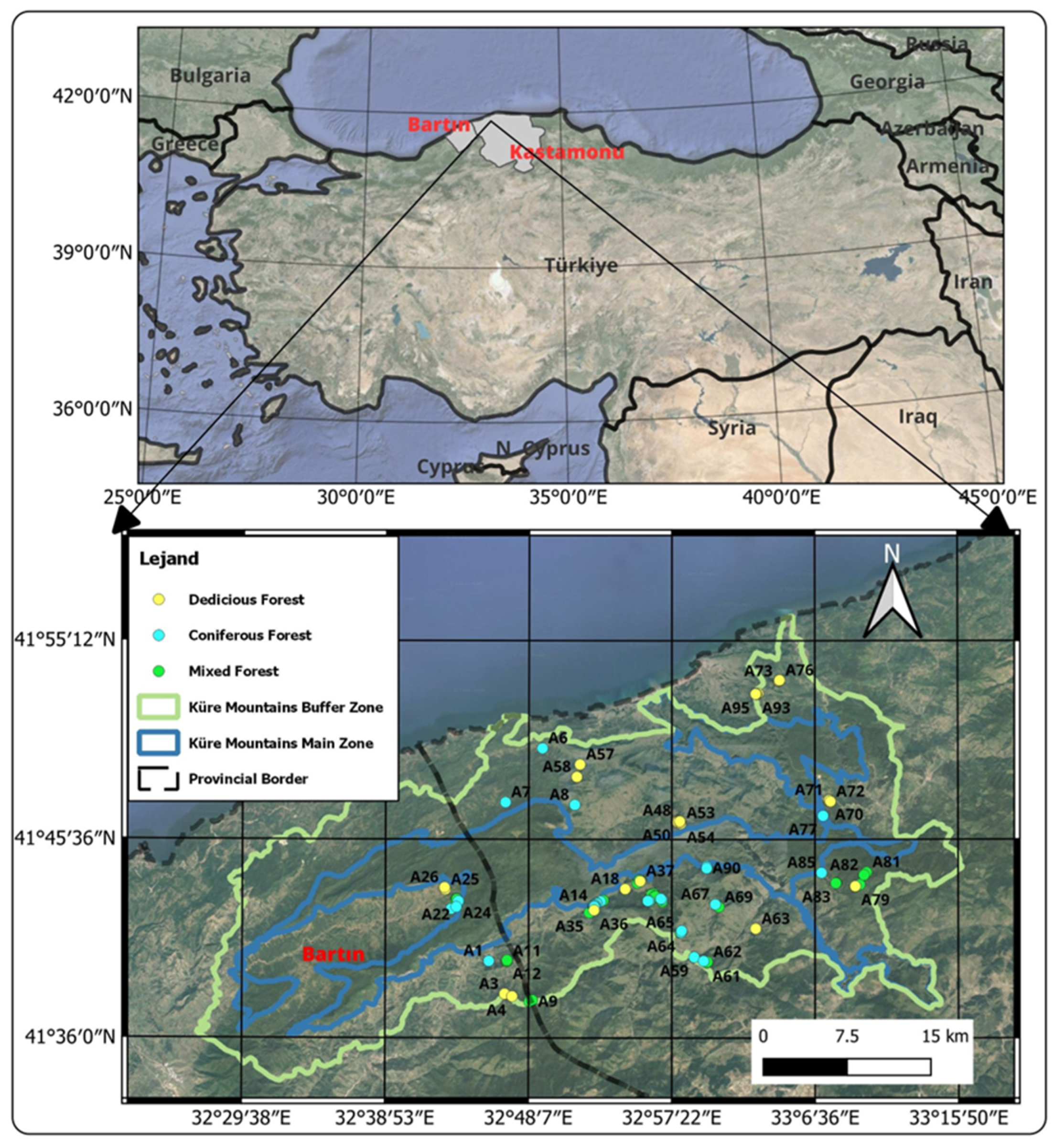
2.1. Study Area

The study area is located within the buffer zone of KMNP, situated in the western region of the Black Sea area, Northern Türkiye, between the latitudes of 41°36′0″–41°55′12″N and longitudes of 32°38′53″–33°15′50″E (Figure 1). The KMNP buffer zone encompasses approximately 134,366 hectares, with an average elevation of 0 to 1650 m.

Surrounding the Küre Mountains, the park encompasses eight districts within Bartın province, including Merkez, Amasra, Kurucaşile, and Ulus, as well as Azdavay, Cide, Pınarbaşı, and Şenpazar districts within Kastamonu. Approximately 52% of the area falls within Bartın. Thirty-seven thousand hectares within this territory were designated the KMNP in 2000 [47]. The climate type is characterized by the Black Sea (temperate maritime climate), with warm summers and mild winters and rainfall occurring almost every season. The region’s proximity to the sea and the alignment of the relatively low mountain ranges parallel to the coast contribute to a reduction in temperature variations along the coastal strip, an increase in humidity, and exposure to air masses from the Balkans [48].

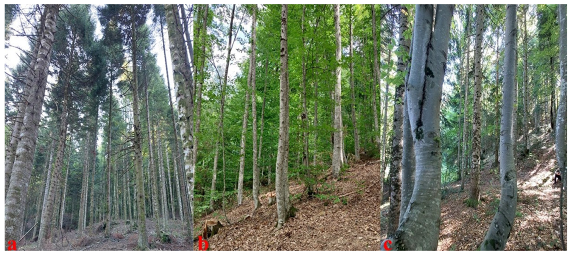
2.2. In-Situ Plot Survey

Fagus orientalis Lipsky, commonly referred to as oriental beech, is a prevalent species naturally distributed in Türkiye. Another species, Fagus sylvatica L. (European beech), is also present in Türkiye, albeit to a lesser extent. Oriental beech is additionally found in Bulgaria, Caucasia, and Iran. Within Türkiye, it is predominantly found in the Black Sea region. As a deciduous species, oriental beech is essential in the country’s forests, accounting for approximately 8.5% of the total forested area, covering about 1.9 million hectares. Renowned for its capacity to yield high-quality wood, characterized by a smooth trunk capable of attaining diameters exceeding 1 m and heights of 30–40 m [49].

Firs are coniferous trees commonly found in forested areas, exhibiting a pyramidal shape in their youth and developing a conical crown as they mature. Türkiye has four native fir species: A. bornmulleriana, A. nordmanniana, A. equi-trojani, and Abies cilicica. Abies nordmanniana subsp. bornmülleriana Mattf. is a prominent fir species native to Türkiye, particularly prevalent in the Uludağ region. This endemic species thrives in Northern Anatolia, specifically in the Western Black Sea Mountains, spanning between Uludağ and the Kızılırmak River, at elevations ranging from 1000 to 2000 m [50].

A total of 95 plots were sampled, encompassing Uludağ fir (29 plots), oriental beech (33 plots), and mixed forests (33 plots) during the field works between July and September of 2022 and 2023 (

Table 1. Statistical summary of the field AGB (t/ha) from the sample plots.

Forest Type	Plots No	Min (t/ha)	Max (t/ha)	Mean (t/ha)	Standard Deviation
Coniferous forest (Uludağ fir)	29	171.274	422.974	323.344	57.022
Deciduous forest (oriental beech)	33	192.650	339.355	253.966	40.528
Mixed forests (Uludağ fir and oriental beech)	33	234.201	391.392	315.421	38.139

).

These plots varied in elevation, aspect, slope, location, and stand development age. The sample areas were delineated in square or rectangular shapes (15 × 10, 15 × 20, 20 × 25, 20 × 30, or 25 × 30 m) with dimensions sufficient to accommodate a minimum of 15 individual trees [51]. Crown cover measurements consistently demonstrated a uniform trend across all sampling plots, indicating significantly larger crown covers (70% and 80%, Closure: 3). The diameter at breast height (DBH) of 1.3 m above the ground (d_1.3) m and height (h) m of each tree was recorded within all sample areas. The images depicting the sampling plots for species-specific AGB estimation within the study area are as follows (Figure 2).

In the context of field studies, Tree diameter was measured in centimeters using a measuring tape or digital caliper, while tree height was measured in meters using a Haglöf EC II Electronic Clino/Height Meter (Haglöf Sweden AB, Långsele, Sweden). Additional data such as central coordinates, terrain elevation, slope, aspect, and slope position were collected alongside d_1.3 (m) and h (m) data from the sampling plots. The central coordinates within the sampling areas were recorded using a Garmin Oregon handheld GPS device (Garmin Ltd., Olathe, KS, USA) utilizing the WGS84 coordinate system. A summary of all collected in situ parameters and their corresponding accuracies is provided in

Table 2. In-situ plot survey parameters.

Parameter	Unit	Measurement Method	Validation Method	Accuracy
Tree Diameter	cm	Measuring Tape, Digital Caliper	Repeated measurement, cross-checking	±0.1–0.5 cm
Tree Height (h)	m	Haglöf EC II Electronic Clino/Height Meter (Långsele, Sweden)	Repeated measurement, cross-checking	±0.2–1.0 m
Central Coordinates	Degrees	Garmin Oregon GPS (WGS84) (Kansas, USA)	Repeated measurement, cross-checking	±3–10 m
Filed Elevation	m	GPS, DEM	Comparison with DEM (SRTM)	±5–10 m (GPS)
Slope (%)	%	DEM, Clinometer	Validation with DEM data, manual measurement	±2–5%
Aspect (°)	°	Magnetic Compass, DEM	Comparison with DEM analysis	±5°

.

2.3. Allometric Growth Equation

Destructive sampling and weighing of entire trees are preferred for providing direct measurements. However, this method is often expensive and labor-intensive for biomass research [52]. Non-destructive techniques primarily rely on biomass equations to estimate tree biomass using measurements of tree diameters and heights obtained through sample assessments. Allometric equations in forestry, which establish relationships between various tree characteristics, are commonly utilized. Through such equations, easily measurable characteristics, like d (m) and h (m), can be used to estimate the volume of entire trees or specific tree components [53].

In this study, the allometric equation used for the estimation of AGB for oriental beech species by Saraçoğlu [54] (1) and for Uludağ fir species by Karabürk [55] (2) are as follows:

Log (AGB) = 2.862640 + 0.012441 × (d_1.3) _i − 14.909870× (d_1.3)) _i ⁻¹ (R = 0.926, S_y,x = 0.149)

(1)

AGB = 84.61739 + (−20.9204 × (d_1.3) + (0.599125 × (d_1.3) × h) + (0.930834× (d_1.3)) + (−0.0114× (d_1.3) × h) (R² = 98.8)

(2)

The term d_1.3 represents the diameter at a height, while h represents the tree height. R signifies the relationship between AGB and d_1.3. S_y,x indicates the standard error of estimate, and R² indicates the coefficient of determination. The distribution of biomass values calculated from the field-sampling sites is depicted in (Figure A1).

2.4. Data Pre-Processing and Variables

Multifrequency SAR satellite data were used, including ALOS-2 PALSAR-2, SAOCOM 1-A, S1, and TSX SAR, for estimating the biomass of a particular area. Multiple processing steps were employed, including calibration to ensure accuracy, speckle filtering to remove the noise inherent in SAR imagery, orthorectification to correct for positional errors, and backscattering coefficient conversion of linear values to decibel values using ESA’s SNAP 9.0 program. Multiple frames for each satellite extensively covered the study area, and consistent methodologies were applied for data processing to ensure accuracy and consistency. The ALOS-2 PALSAR-2 data, which offer full polarimetric modes (horizontal–horizontal (HH), horizontal–vertical (HV), vertical–vertical (VV), vertical–horizontal (VH)), were obtained from the Japan Aerospace Exploration Agency (JAXA). The acquisition date for the ALOS-2 PALSAR-2 imagery was August 10, 2023. Pre-processing of the data involved several steps, including calibration to ensure data accuracy, despeckle Lee filtering (filter size 5 × 5) to enhance image quality by reducing speckles, and orthorectification and re-projection to WGS84 (EPSG:4326) to correct geometric distortions using range Doppler terrain correction (SRTM 1-Arc Second DEM) and standardize the projection system.

The SAOCOM 1A satellite managed and operated by CONAE (Comisión Nacional de Actividades Espaciales), Argentina’s Space Agency, was launched in 2018. The study area is covered by four frames, with the dual polarimetric images (HH, HV) acquired on 20 August 2023 and 23 August 2023. Comparable processing methodologies were employed for the data obtained from both satellites, mirroring the procedures applied to ALOS satellite data. The preprocessing included radiometric calibration, resampling to a 10 m resolution, and terrain correction based on DEM. Despeckle Lee filtering was applied to minimize noise while maintaining backscatter integrity. The final dataset regarding the HH and HV polarimetric backscattering coefficients, which were subsequently utilized for biomass estimation, was analyzed.

The S1 SAR image ground range detected (GRD data) acquired on 12 August 2023 underwent several processing steps, including the application of precise orbit files, thermal noise removal, radiometric calibration, and terrain correction using the WGS84 reference system. Additionally, Lee speckle filtering was applied to reduce noise while preserving essential textural features. Subsequently, backscattering coefficients were converted to decibels (dB) and tested for VV and VH polarimetric backscattering values for biomass estimation.

TSX is a radar satellite from DLR (the German Aerospace Center) launched in 2007. The study area is covered by three frames, each encapsulating dual polarimetric TSX images (HH, VV) acquired on 28 July 2023, 8 August 2023, and 19 August 2023. The processing steps included radiometric calibration, resampling to a standardized 10 m resolution, and terrain correction to rectify geometric distortions—Despeckle Lee filtering enhanced signal quality by reducing speckle noise while preserving the structural information. The final dataset included backscatter coefficients for HH and VV polarizations, which were subsequently analyzed for their contribution to biomass estimation. In the final step for all SAR images, the backscattering values (σ°) were converted using a logarithmic transformation provided in Equation (3). Details regarding the satellite images are provided in

Table 3. Detailed specifications of multifrequency SAR data.

Sensor	Band	Pass	Polarization	Range Resolution (m)	Azimuth Resolution (m)	Acquired Date
TerraSAR-X	X	Ascending	HH, VV	0.91	2.42	28 July 2023, 8 August 2023, 19 August 2023 (3 frames),
Sentinel-1A (GRD)	C	Descending	VH, VV	20	22	12 August 2023
SAOCOM 1A	L	Descending	HH, HV	4.75	4.99	20 August 2023 (2 frames), 23 August 2023 (2 frames)
ALOS-2 PALSAR-2	L	Descending	HH, HV, VH, VV	2.86	3.12	10 August 2023

.

σ° dB= 10 × log(σ°)

(3)

Optical images acquired by Sentinel-2A on 23 August 2023, were subjected to level 2A bottom-of-atmosphere (BOA) reflectance processing, signifying the application of atmospheric and geometric corrections, thereby ensuring the inclusion of surface reflectance values within the bands. These bands were resampled to a 10 m resolution. Band values were employed to compute vegetation indices, while texture measurements were derived using the SNAP 9.0 program. Forty predictive variables were extracted for this study, including the polarizations of radar images, the bands of optical images, optical vegetation indices, texture measures, and topographic variables. Detailed information concerning the bands, vegetation indices, and GLCM texture measurements for the optical image is available in

Table 4. Detailed parameters of multispectral optical data, vegetation indices, texture measures, and topographic variables.

Variable Types	Variable Number	Variable Names	Description	References
Sentinel-2A	12	Bands	B1, B2 (Blue), B3 (Green), B4 (Red), B5, B6, B7 (Vegetation Red Edge), B8 (NIR), B8a, B9, B11, B12	-
Vegetation Indices		CVI	Chlorophyll vegetation indices (B4 × B8)/(B3 × B3)	[56]
		EVI	Enhanced Vegetation Indices 2.5*(B8 − B4)/(B8 + 6 ×B4 − 7.5*B2 + 1)	[57]
	5	PSSRA	The Pigment Specific Simple Ratio a (B7/B4)	[58]
		TNDVI	Transformed Normalized Difference Vegetation Indices ([(B8 − B4)/(B8 + B4)] + 0.5)0.5	[59]
		MSR	Modified Simple Ratio [B4/(B8/B4 + 1)0.5]	[60]
Texture Measures	10	“TjMea, TjVar, TjHom, TjCon, TjM TjDis, TjEn,TjEnt, TjASM, TjCor”	TjXXX represents a texture image developed in the S2 band using the texture measure XXX with a j × j (j = 5) pixel window, where XXX is Mea (Mean), Var (Variance), Hom (Homogeneity), Con (Contrast), M(Max), Dis (Dissimilarity), En (Energy), Ent (Entropy), ASM (Angular Second Moment), or Cor (Correlation).
Topographic Variables	3	slope, aspect, altitude	Shuttle Radar Topography Mission (SRTM) 1 Arc Second DEM

, with the preprocessing steps elucidated in the workflow diagram depicted in Figure 3.

For the pre-processing of the optical and radar images, data analysis was initiated by computing the arithmetic mean of the band reflectance values within pixels encompassed by polygons delineating each area. This computation was performed using the QGIS 3.28 GIS program. Polygons of 5 m × 5 m dimensions were created to account for potential inaccuracies in the coordinates of the sampling areas, as the central coordinates were obtained using a handheld GPS, which may introduce positional errors. Specifically, by averaging the values at the four corners of each 5 m × 5 m polygon, we obtained a more robust estimate of AGB, mitigating the impact of GPS-induced positional shifts on the alignment between field data and satellite observations. The area of each plot was calculated and subsequently converted to hectares to facilitate standardized biomass estimation and analysis.

2.5. Feature Selection Methods

Feature selection constitutes a critical preprocessing step within ML, aimed at discerning essential features by eliminating irrelevant or redundant elements from the original feature set. Many feature selection algorithms prioritize the maximization of pertinent information while minimizing redundancy. To enhance the evaluation criteria’s efficacy in eliminating redundant information, emphasis is placed on refining the selection process further [61,62].

2.5.1. Mutual Information

The feature selection algorithm based on mutual information (MI) selects essential features from the original data set to remove irrelevant and redundant features. It operates on the intuitive premise that higher mutual information indicates a more substantial contribution to prediction. Diverging from the limitations of Pearson linear correlation, MI excels in capturing nonlinear relationships between variables. The MI algorithm solely evaluates the correlation between features and the class label, facilitating the elimination of irrelevant features. However, it does not account for the interrelation between candidate features and the already selected feature subset. Consequently, in scenarios where datasets encompass numerous redundant features, the classification accuracy of this algorithm tends to diminish [63,64,65].

2.5.2. Recursive Feature Elimination

RFE is a widely acclaimed wrapper crafted to meticulously identify the most advantageous subset of features. This method meticulously iterates through the construction of models, selecting the optimal predictive feature set along the way. Features are methodically eliminated or retained at each iteration based on their coefficients’ performance metrics [66]. Through this iterative process, the model dynamically adjusts, strategically discarding either the best-performing or least-contributing features until the most pertinent subset is derived. The most salient residual features form the foundation for constructing subsequent models, perpetuating the refinement process until all relevant features have been considered. A robust resampling technique, such as 10-fold cross-validation, is commonly employed with RFE to gauge the optimal number of features. This rigorous approach ensures the reliability and generalizability of the selected feature subset, minimizing the risk of overfitting and maximizing predictive performance [67].

2.5.3. LASSO Regularization

LASSO represents an alternative LR technique renowned for its regularization capabilities. Through regularization, LASSO effectively identifies and eliminates extraneous predictors during model construction, ensuring that only pertinent predictors are retained. This attribute enables LASSO to furnish a streamlined set of predictors, enhancing the model’s interpretability and accuracy [68]. A rigorous 10-fold cross-validation approach was adopted, systematically partitioning the dataset into subsets for training and validation to ascertain the robustness and generalizability of the regression model.

2.6. Regression Models

2.6.1. Multivariate Linear Regression

MLR is a statistical methodology that delineates the relationship between multiple independent variables and a dependent variable, encapsulating the linear relationship within a unified functional expression. Unlike simple LR, which examines the connection between a single independent variable and a dependent variable, MLR recognizes the impact of multiple independent variables in elucidating various natural phenomena. The MLR model is expressed as Equation (4) below:

Y_i = β₀ + β_1xi1 + β_2xi2 +…+ β_pxip + ϵ_i

(4)

where β denotes the constant term, x represents the coefficients of variables in the model, and ε signifies the residual error. In an LR algorithm encompassing multiple variables, it is assumed that there exist p independent variables [69].

2.6.2. LASSO Regression

LASSO regression, introduced by Robert Tibshirani [70], presents a novel approach to variable selection. Operating as a shrinkage estimation model, its objective is to minimize the sum of squares of residuals while imposing a constraint on the absolute values of the regression coefficients, ensuring that their sum remains below a constant threshold. This constraint induces some regression coefficients to become strictly equal to zero, resulting in more interpretable models. Particularly advantageous in scenarios involving numerous variables or sparse variable matrices, LASSO demonstrates clear benefits. By utilizing penalty functions, LASSO achieves shrinkage estimation, compelling certain variable coefficients to be zero. This not only simplifies the model but also mitigates the risk of overfitting [71,72].

2.6.3. Ridge Regression

The ridge regression model was introduced by Hoerl and Kennard [32,73] and addresses the issue of instability or inactivation encountered in least squares estimation within MLR algorithms. This instability arises from the presence of collinearity among independent variables. Ridge estimation of coefficients in an LR algorithm aims to mitigate these challenges. The ridge model is expressed as Equation (5) below:

$$\widehat{\beta }\left(k\right)={\left(X^{\prime }X+kl\right)}^{-1}{X}^{\prime }Y$$

(5)

where X represents an n x p matrix of the independent variable, X’ denotes the transpose of X, l stands for an n x n identity matrix, Y is an n x 1 vector of observations (biomass), and k signifies a scalar constant (the ridge parameter).

2.6.4. PLS Regression

PLSR was developed by Wold et al. [33] and is a regression model that utilizes latent variables selected to maximize the correlation between predictors and the response variable. This approach involves extracting a set of orthogonal factors from independent variables, prioritizing those with the strongest predictive power to meet the modeling objectives effectively. PLSR extends conventional MLR algorithms by integrating principles from both principal component analysis and canonical correlation analysis. Additionally, PLSR incorporates cross-validation techniques to assess the robustness and performance of its regression model [74]. PLSR incorporates a crucial variable selection process referred to as variable importance in projection (VIP) (Equation (6)), which assesses the explanatory power of individual independent variables concerning the dependent variable.

$$V_{IP}=\sqrt{{\displaystyle \frac{k}{\sum _{h=1}^n{r}^2\left(y,ch\right)\sum _{h=1}^n{r}^2(y,ch){w_{hj}}^2}}}$$

(6)

where k represents the number of independent variables, ch signifies the principal component extracted from the independent variables, r²(y,ch) denotes the correlation coefficient between the dependent variable and the principal component, and w_hj represents the weight of the independent variable in the principal component [37].

2.7. Model Accuracy and Statistical Analysis

The field dataset, consisting of 95 observations, was partitioned into a training dataset comprising 70% of the data and a test dataset comprising 30%. This partitioning facilitated the training of four empirical models using a specific subset of samples, followed by the assessment of model performance in predicting AGB using a separate set of samples dedicated to testing.

The efficacy of each model was assessed by comparing the predicted AGB values against the measured AGB values in the testing dataset. Three standard metrics were employed to evaluate the accuracy of the predictions: root mean square error (RMSE), coefficient of determination (R²), and mean absolute error (MAE). RMSE, a widely utilized metric, quantifies the discrepancies between the predicted values generated by a model and the corresponding observed or measured values.

$$\mathrm{RMSE}=\sqrt{{\displaystyle \frac{1}{\mathrm{n}}}{\sum }_{\mathrm{i}=1}^{\mathrm{n}}{\left(\widehat{\mathrm{y}}\mathrm{i}-\mathrm{y}\mathrm{i}\right)}^2}$$

(7)

$${\mathrm{R}}^2=1-{\displaystyle \frac{{\sum }_{i=1}^n{\left(x_i-\widehat{\mathrm{y}}i\right)}^2}{{\sum }_{i=1}^n{\left({\overline{y}}_i-y_i\right)}^2}}$$

(8)

$$\mathrm{MAE}={\displaystyle \frac{1}{\mathrm{n}}}{\sum }_{\mathrm{i}=1}^{\mathrm{n}}\left|\left(\widehat{\mathrm{y}}\mathrm{i}-\mathrm{y}\mathrm{i}\right)\right|$$

(9)

where $\widehat{\mathrm{y}}\mathrm{i}$ and yi, respectively, represent the predicted AGB and measured AGB of the plot, ${\overline{y}}_i$ denotes the mean value of AGB, and n is the total number of plots. A smaller RMSE indicates higher accuracy. R² signifies the extent to which the model elucidates the observed AGB values, representing the proportion of total variation in AGB that can be accounted for by the model. All of the training data were utilized to train the AGB model, and 30% of the test data were employed to evaluate its performance for AGB estimation.

3. Results

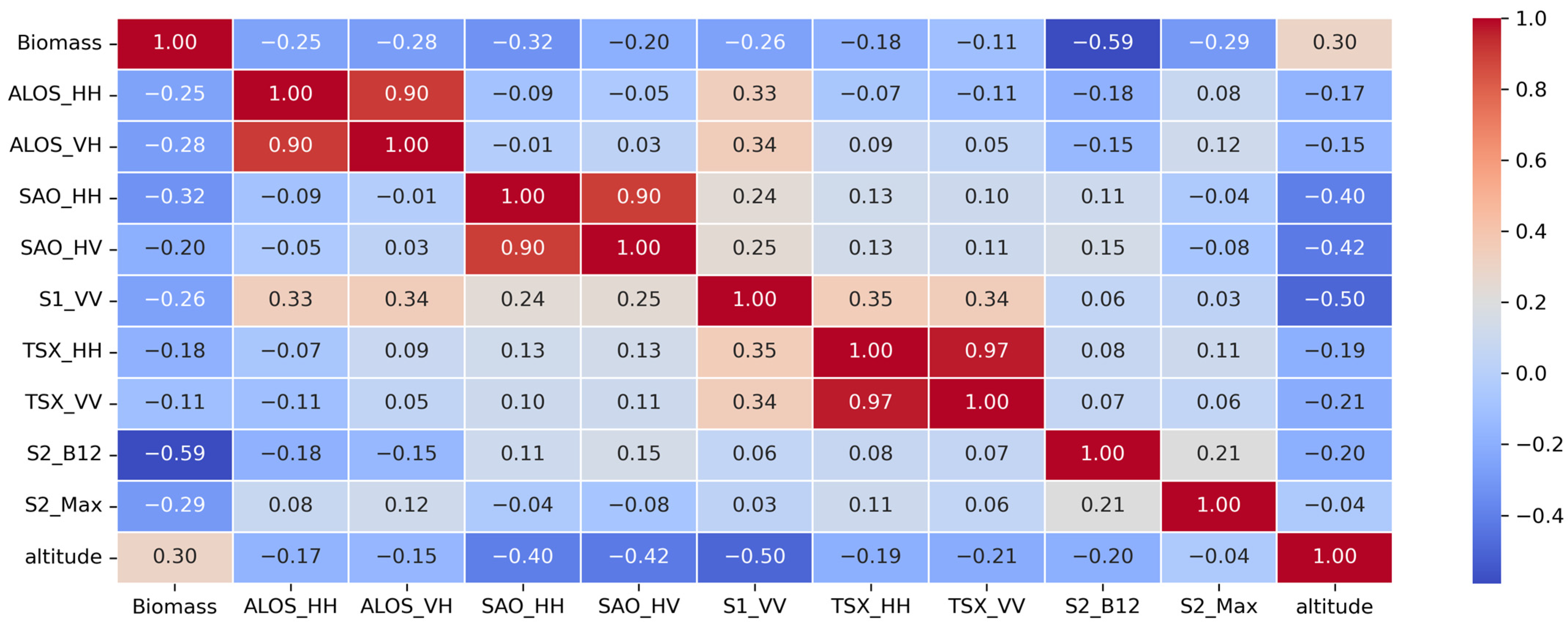
3.1. Statistical Analysis

The results, with a significance level of α = 0.05 and a p-value of less than 0.05, indicate statistical significance. The high R² and multiple R values indicate that the model effectively explains the dataset, while the low standard error suggests accurate predictions by the model. The F-value of 21.276, obtained for the one-way analysis of variance (ANOVA) test that assessed the statistical significance of the regression model, indicates a significant difference among groups. The significance of 4.258 × 10⁻¹⁹ (or approximately zero) confirms that this difference is statistically significant (

Table 5. Regression statistics and ANOVA.

Regression Statistics
Multiple R			0.847
R squared			0.717
Adj. R squared			0.683
Standard Error			30.857
Observation			95
ANOVA
	df	SS	MS	F	Sig.
Regression	10	202,584.479	20,258.448	21.276	4.258 × 10⁻¹⁹
Differences	84	79,981.354	952.159
Total	94	282,565.833

).

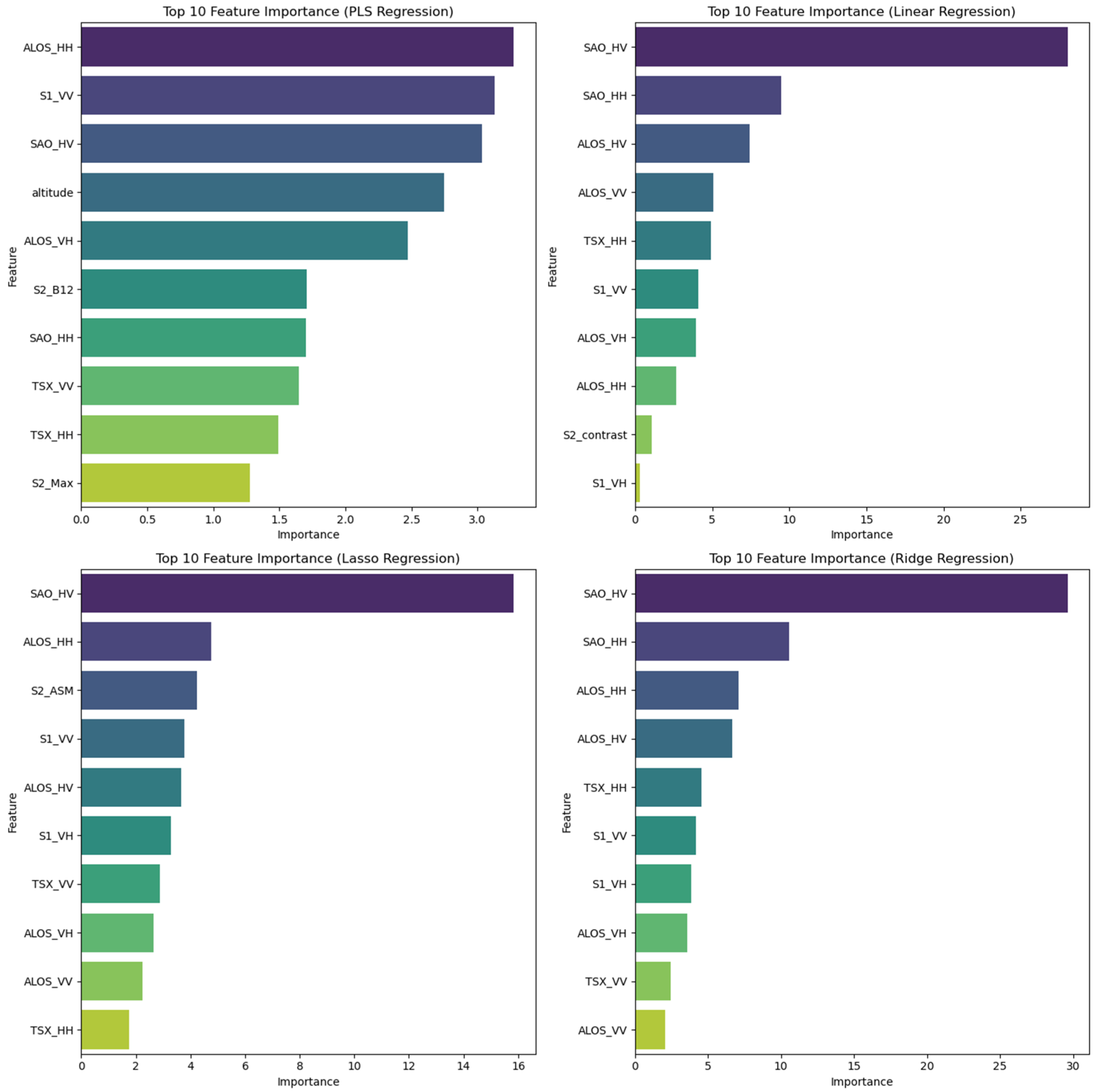
3.2. Analyzing Selecting and Important Predictors for AGB Estimation

In this study, three distinct feature selection methodologies, namely MI, RFE, and LASSO regularization were implemented using the Python 3.8 Scikit-learn library 1.5.2 (https://scikit-learn.org/1.5/) (accessed on 8 November 2024).Three feature selection methods were applied to identify different subsets of features. We employed statistical scores of the regression models as our judging criteria. Subsequently, the method demonstrating superior performance relative to the others was selected to curate the optimal feature set. The feature selection process entailed calculating the highest R² value between the feature variables and the AGB data, thereby identifying the most optimal model. To ensure robustness, each selected feature subset was assessed using a RandomForestRegressor model, trained on the training dataset, and evaluated on an independent test set. Ultimately, the subset achieving the highest R² score was chosen as the final feature set, ensuring a rigorous validation process through multiple selection techniques, independent testing, and cross-validation (CV). The performance of each feature set was assessed based on the R² score. Additionally, cross-validation was employed within the feature selection process (e.g., RFECV and LassoCV) to mitigate overfitting and enhance generalizability. Ultimately, the feature subset yielding the highest R² score was chosen as the final set, demonstrating that the selection process was validated not only through multiple feature selection techniques but also via independent testing and cross-validation. Emphasizing the most successful among the three feature selection methods, LASSO stands out for its efficacy; 30 variables were eliminated from the initial pool of 40 predictive variables (R² = 0.61). The correlation map is shown in Figure A2.

The coherence and significance level of the features employed in AGB estimation regression models is of paramount importance. The impact of the feature selection methods utilized here is undeniable. As depicted in Figure A3, the predictor variables employed in the models exhibit the highest accuracy, highlighting the importance of the top 10 features across all regression models. Notably, within the PLSR model, it was discerned that the intercepts of ALOS-2 PALSAR-2 HH, S1 VV, and SAOCOM HV polarizations were recurrently chosen over the other predictor variables. ALOS-2 PALSAR-2 VH, SAOCOM HH, TSX VV, TSX HH polarizations, S2 optical band 12, altitude, and S2 Max are the top ten and also hold considerable importance in the predictive modeling of PLSR. Furthermore, across all regression models, the notable contribution of SAOCOM-HV polarization to the level of importance is evident.

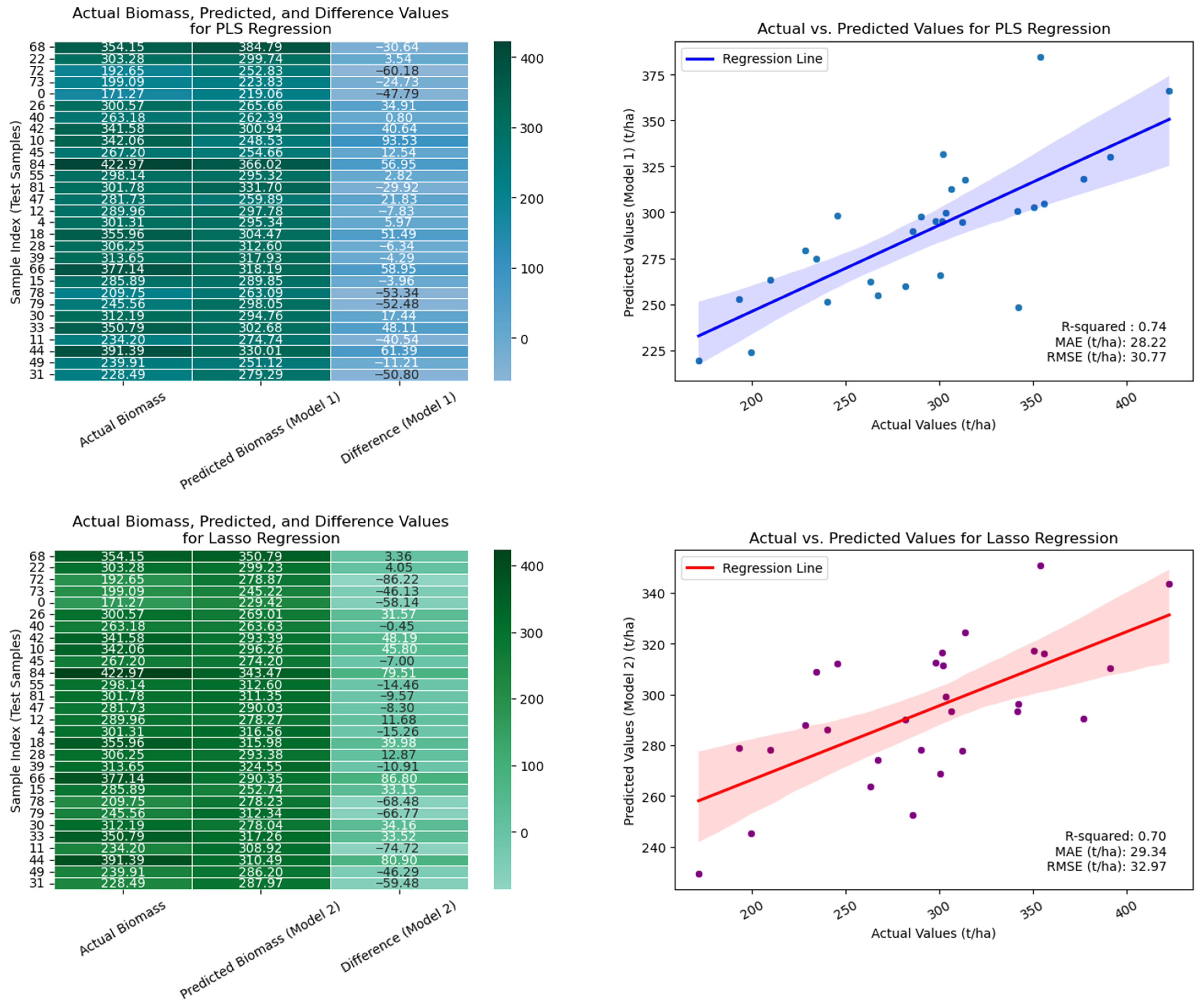
3.3. Mapping AGB and Regression Analysis

This study employed multiple ML algorithms, each configured with distinct predictor variables, to map AGB. The outcomes derived from the test phase reveal a notably enhanced predictive capacity, as evidenced by a heightened R², alongside reduced RMSE and MAE values in the context of AGB estimation. Particularly noteworthy is the proficiency of the PLSR model, which emerged as the most effective in AGB estimation within the study area (R² = 0.74, MAE = 28.22 t/ha, RMSE = 30.77 t/ha). It is worth mentioning that LASSO regression (R² = 0.70, MAE = 29.34 t/ha, RMSE = 32.97 t/ha) and MLR algorithm exhibited comparable efficacy to PLSR (R² = 0.69, MAE = 29.43 t/ha, RMSE = 33.37 t/ha). Among the evaluated models, ridge regression demonstrated the least successful performance (R² = 0.53, MAE = 35.60 t/ha, RMSE = 36.04 t/ha).

The analysis of the 12 models presented in

Table 6. Evaluation of different satellite data combinations in predictive regression models. ‘S2_B12’ refers to Sentinel-2 band 12 (SWIR—shortwave infrared), while ‘S2_Max’ represents the Sentinel-2 band using the texture measure with a j × j (j = 5) pixel window, where Max stands for maximum. ‘VV’ (vertical–vertical) and ‘HV’ (horizontal–vertical) indicate the polarization modes of radar data. ‘ALOS’ corresponds to ALOS-2 PALSAR-2 L-band radar data. ‘SAO’ represents SAOCOM radar data, ‘S1’ shows Sentinel-1, and ‘TSX’ refers to TerraSAR-X radar data. ‘Altitude’ indicates terrain elevation. The parameters listed within brackets [ ] represent different feature combinations used in the models.

		PLSR			LASSO Regression			MLR			Ridge Regression
Model	Features	R2	RMSE	MAE	R2	RMSE	MAE	R2	RMSE	MAE	R2	RMSE	MAE
1	[‘S2_B12’, ‘S2_Max’]	0.24	52.73	45.24	0.26	51.97	44.71	0.25	52.46	44.75	0.13	56.26	45.13
2	[‘ALOS_HH’, ‘SAO_HH’, ‘S1_VV’]	0.26	51.90	43.29	0.27	51.75	43.27	0.27	51.78	43.27	0.25	52.26	43.30
3	[‘ALOS_HH’, ‘SAO_HH’, ‘TSX_HH’, ‘S1_VV’]	0.29	50.83	42.84	0.29	50.79	42.73	0.29	51.06	42.84	0.28	51.26	42.93
4	[‘ALOS_HH’, ‘ALOS_VH’, ‘TSX_HH’, ‘S1_VV’, ‘S2_Max’, ‘altitude’]	0.33	49.57	39.38	0.28	51.36	40.30	0.18	54.83	45.62	0.28	51.24	40.90
5	[‘ALOS_VH’, ‘TSX_HH’, ‘TSX_VV’, ‘S1_VV’, ‘S2_B12’, ‘S2_Max’, ‘altitude’]	0.44	45.03	36.60	0.54	41.12	33.76	0.51	42.08	34.70	0.38	47.70	39.86
6	[‘ALOS_HH’, ‘ALOS_VH’, ‘TSX_HH’, ‘TSX_VV’, ‘S1_VV’, ‘S2_B12’, ‘altitude’]	0.51	42.34	34.12	0.55	40.57	33.24	0.53	41.59	34.52	0.35	48.76	42.40
7	[‘SAO_HH’, ‘SAO_HV’, ‘TSX_HH’, ‘S1_VV’, ‘S2_B12’]	0.53	41.31	35.13	0.53	41.31	35.13	0.52	42.04	35.67	0.37	47.79	39.81
8	[‘ALOS_HH’, ‘SAO_HH’, ‘TSX_VV’, ‘S1_VV’, ‘S2_B12’, ‘S2_Max’, ‘altitude’]	0.61	37.96	30.89	0.61	37.96	30.84	0.58	38.95	31.37	0.44	45.16	35.80
9	[‘ALOS_HH’, ‘ALOS_VH’, ‘SAO_HH’, ‘TSX_HH’, ‘TSX_VV’, ‘S2_B12’, ‘S2_Max’, ‘altitude’]	0.63	36.74	30.56	0.61	37.71	31.72	0.59	38.65	32.56	0.44	45.14	35.89
10	[‘ALOS_HH’, ‘ALOS_VH’, ‘SAO_HH’, ‘SAO_HV’, ‘TSX_HH’, ‘S2_B12’, ‘altitude’]	0.70	32.87	28.35	0.69	33.41	28.72	0.68	33.91	29.05	0.49	43.02	36.80
11	[‘ALOS_HH’, ‘ALOS_VH’, ‘SAO_HH’, ‘SAO_HV’, ‘TSX_HH’, ‘TSX_VV’, ‘S2_B12’, ‘S2_Max’, ‘altitude’]	0.72	31.84	28.04	0.69	33.38	28.70	0.69	33.75	29.84	0.51	42.47	36.99
12	[‘ALOS_HH’, ‘ALOS_VH’, ‘SAO_HH’, ‘SAO_HV’, ‘TSX_HH’, ‘TSX_VV’, ‘S1_VV’, ‘S2_B12’, ‘S2_Max’, ‘altitude’]	0.74	30.77	28.22	0.70	32.97	29.34	0.69	33.37	29.43	0.53	36.04	35.60

indicates that AGB estimation based solely on optical or radar data consistently yields low results across all four regression models, exhibiting similar outcomes. The discernible positive impact of S2 band 12 begins to manifest from Model 5 onwards, leading to a notable enhancement in the results. While the incorporation of TSX in Model 8 may not individually exert a substantial effect, it generally contributes to improvement. In Model 11, the inclusion of the S2 texture measure, S2 Max, demonstrates a significant improvement in the AGB estimation results. S1 data and altitude features are observed to have a notably beneficial effect, which is particularly evident in Model 12. Additionally, L-band ALOS-2 PALSAR-2 and SAOCOM satellite data demonstrate high effectiveness in AGB estimation, especially when combined, thereby offering augmentative effects. Remarkably, SAOCOM HV and ALOS-2 PALSAR-2 HH polarizations exhibited exceptional efficacy across all models, and the values are also depicted in Figure 4.

The estimations and corresponding graphs for the predictive values obtained from the combination comprising ALOS-2 PALSAR-2 HH and VH, SAOCOM HH and HV, TSX HH and VV, S1 VV polarizations, S2 band 12, S2 Max texture measure, and altitude, encompassing the most successful regression models, PLSR and LASSO regression, are depicted in Figure 5. The sample index on the vertical axis represents the different sampling-area numbers used for test data in the regression models. These correspond to specific biomass measurements, where each row indicates the actual biomass value alongside the predicted values from the PLSR and Lasso regression models. The difference column represents the discrepancy between the actual and predicted biomass values (t/ha) in Figure 5.

Our results indicated that the accuracy of the AGB estimates from the model was comparable to the PLSR and LASSO regression models. Upon comparing the predicted biomass values generated by the PLSR and LASSO regression models with the actual biomass values, it becomes evident that both models exhibit a linear and closely aligned trend, particularly within the range of 250 to 350 t/ha. This observation is depicted in Figure A4, where the PLSR and LASSO regression predicted values demonstrate proximity to the ideal reference line of equality. The results indicate a tendency towards producing predictions closer to the actual values, as evidenced by the residuals being closer to zero within this range. This suggests that both the PLSR and LASSO regression models offer promising performance in approximating the actual biomass values within this specified range, signifying their efficacy in biomass prediction tasks. The map illustrating AGB generated by the PLSR is presented in Figure 6.

4. Discussion

4.1. Feature Selection Methods and Impact on AGB Estimation

Feature selection is a crucial preprocessing step in ML that is aimed at identifying essential features by eliminating irrelevant or redundant elements from the original feature set. This process has been widely utilized in numerous studies, including those employing correlation feature selection, MI, RFE, RFE with cross-validation (RFECV), LASSO, genetic algorithm, and Boruta algorithm [75,76,77,78,79]. In our study, we employed three feature selection methods, namely MI, RFE, and LASSO, to prepare the optimal dataset for AGB estimation. Among these methods, LASSO yielded the most favorable results (R² = 0.61), indicating its effectiveness in selecting pertinent features for accurate estimation. Similar findings have been reported in other studies, further validating the efficacy of the LASSO method in similar contexts [80,81].

4.2. Performance of Machine-Learning Regression Models

The feature parameters of ML models are not limited by dimensionality, and the inversion of forest total biomass using ML models has good robustness when there is multicollinearity between the feature variables, effectively avoiding the loss of important parameters while maintaining excellent estimation performance [82]. Moreover, ML is extensively employed for accurately estimating AGB [26,27,31]. This study conducted a comparative analysis of four ML regression models for the estimation of AGB using various satellite data products and ancillary information. The findings indicated that three of the regression models, namely PLSR, LASSO regression, and MLR, exhibited comparable accuracies in estimating AGB, outperforming the ridge regression model. The results indicated that the regression models could enhance the accuracy of estimation, which aligns with findings from several studies [36,83,84,85,86,87].

The estimation of AGB has traditionally relied heavily on ground-based methodologies. However, the emergence of satellite technologies has significantly elevated the significance of research employing remote-sensing techniques, leading to their widespread adoption. Optical satellite data (S2 and Landsat series) are predominantly utilized, alongside S1 C band and ALOS-2 PALSAR-2 dual or mosaic radar satellite data, for AGB estimation. Sakici and Günlü [88] employed Landsat-8 optical satellite data to model forest parameters utilizing MLR and artificial neural networks (ANN). Their findings indicated that ANN yielded superior results compared to MLR. Pham et al. [27] showed that a combination of S1, S2, and ALOS-2 PALSAR-2 data can estimate the mangrove AGB with promising accuracy (R² = 0.68) and ALOS-2 PALSAR-2 sensor makes a more important contribution. The choice of modeling approaches significantly impacts AGB estimation. MLR is commonly employed, alongside ML methods such as SVR, decision trees, and KNN [38,39]. Recent studies have shown promising results in AGB modeling with algorithms like XGBoost, CatBoost, and RF [25,27,30,79,87]. Cai et al. [83] conducted a study in China’s Mu Us Desert region, comparing ridge regression and PLSR for biomass prediction using Landsat ETM+ imagery and field data. Their results indicated that PLS regression provided the highest accuracy, with an RMSE of approximately 61%. In comparison, ridge regression showed lower accuracy (RMSE: 64%) and poor performance in the full ridge model (RMSE: 87%). Similarly, in our study, we evaluated different satellite data combinations for biomass estimation, finding that PLS regression outperformed other models in terms of accuracy. Morais et al. [89] indicated the prospective application of ML methodologies, including MLR, LASSO, ridge regression, random forests, XGBoost, and LightGBM, in conjunction with S2 data for the estimation of grassland biomass in Portugal. Their investigation revealed that XGBoost and LightGBM algorithms outperformed other ML techniques, yielding a notably superior result with an R² value of 0.81. Chen et al. [37] introduced an ensemble model for AGB estimation, integrating a neural network-optimized back propagation (BP) model termed, PLSR, SVR, and RF regression. This ensemble approach utilized Landsat 8 Operational Land Imager (OLI) and Sentinel-1A data in the central Jiangxi Province, located in Southwestern China, identified Tent_ASO_BP as the most effective regression model, yielding an R² value of 0.74.

Keles et al. [90] focused on AGB estimation for Scots pine in Ankara, Türkiye, utilizing S1–S2 satellite imagery and MLR, SVR, and deep-learning models. SVR emerged as the most effective model among the tested methodologies. Textural data emerges as an additional influential variable contributing to AGB estimation, a phenomenon observed across both optical imagery studies [91] and SAR image analyses [92]. Our study distinguishes itself by incorporating additional satellite imagery beyond S1 and S2, specifically TSX, ALOS-2 PALSAR-2 full polarization, and SAOCOM L-band data.

4.3. Role of Multifrequency Bands and Polarizations in Biomass Prediction

SAR backscatter has been widely employed for estimating AGB in forested areas, leveraging diverse SAR datasets acquiring X-, C-, S-, L-, and P-band frequencies [13,15,17,93,94,95]. In our study, when different bands, polarizations, and their combinations were examined (Table 6), the models incorporating L-band satellites, such as ALOS and SAOCOM (e.g., Model 8 and subsequent models), demonstrated a significant increase in R² values (from 0.53 to 0.74) and a reduction in RMSE and MAE values. This indicates that the higher penetration capability of the L-band allows for better vegetation penetration and provides more consistent results in AGB estimation. Although models incorporating the C-band (S1) and X-band (TSX) exhibited lower R² values, it was observed that their combination with the L-band generally resulted in better penetration and more consistent results due to reduced surface reflection effects in dense vegetation. Notably, Model 12 achieved the highest performance in AGB estimation with the inclusion of S1_VV, leading to an increase in R² from 0.72 to 0.74. Similar to our study, Sandberg et al. [16] demonstrated that HV polarization yields better results in L-band imagery than HH polarization. Also, our findings support the results of Englhart et al. [95], who conducted AGB estimation in Indonesian tropical forests using TSX and ALOS PALSAR L-band satellite images, noting that the relationship between AGB and ALOS data was superior to that of TSX imagery, and the combination of both images resulted in enhanced performance. Our findings are consistent with those that Blomberg et al. [96] presented that employing SAOCOM-CS tomography with a single polarization (HH) significantly enhances biomass retrievals in forests, resulting in error reductions ranging between 26% and 30%. However, the inclusion of SAO_HV in our model resulted in a notable improvement in AGB estimation accuracy (an increase in R² from 0.63 to 0.70, while RMSE and MAE decreased) respectively.

Moreover, studies employing combinations of satellite images have shown that the saturation issue is largely resolved, leading to increased accuracy in biomass estimation [14,97]. In a study by Nuthammachot et al. [98], AGB estimation was conducted using S1 and S2 satellite images in 45 sampling areas, where the coefficient of determination was R² = 0.34 for radar image backscatter values alone, R² = 0.82 for S2 data alone, and R² = 0.84 for the combination of both images using the Normalized Difference Index 45 (NDI45), band 6, and VH backscatter. The study highlighted that C-band radar backscatter values alone did not yield satisfactory results in biomass estimation, while the combination of radar and optical imagery produced superior outcomes. Our study highlights the significant impact of ALOS_VH and SAO_HV polarizations, aligning with the findings of Morin et al. [99], who reported that combinations of S1, S2, and ALOS-2 PALSAR-2 yielded the best results and that L-HV polarization is particularly sensitive to wood volume. Additionally, other polarizations, such as HH, further contributed to enhancing overall performance in our study. Vatandaşlar and Abdikan [100] conducted a study to determine total carbon stocks using dual-polarization (HH, HV) mosaic satellite images of S1 and ALOS-2 PALSAR-2, noting that ALOS-2 HH polarization (R² = 0.78) outperformed S1 VH polarization (R² = 0.74). Georgopoulos et al. [101] conducted AGB estimation in needle-leaved forests using S1 and S2 images, highlighting that the highest coefficient of determination (R² = 0.74) was achieved when only radar images were used, with an R² of 0.63 for optical images and an R² of 0.73 for the combination of both images, additionally emphasizing the high correlation obtained with the normalized difference vegetation indices (NDVI) and VH texture features (e.g., VH_GLCMVariance, VH_MAX, and VH_Entropy). In contrast, our study diverged in its approach by focusing on optical imagery (S2) rather than radar texture measures. The S2_Max model significantly contributed to enhancing prediction accuracy in our analysis. Notably, the success of maximum texture measures emerges as a compelling point of convergence between the two studies. Khati and Singh [102] found that a synergistic combination of L-band PolSAR (backscatter) and X-band PolInSAR (height) products provides the best-case AGB inversion with an R² = 0.78. In our study, we found that a combination of L-band ALOS-2 PALSAR-2, SAOCOM, C-band S1, X-band TSX, S2 optical data, and altitude, along with optical texture measure, yielded the most favorable results (R² = 0.74, MAE = 28.22 t/ha, RMSE = 30.77 t/ha). Ji et al. [15] conducted an extensive investigation utilizing 15 combinations of X, C, L, and P band SAR observations for AGB estimation. The study employed multivariate linear stepwise regression (MLSR), RF, and a deep-learning algorithm for analysis. Among these methodologies, the MLSR algorithm incorporating combined L and P band SAR observations exhibited the most favorable performance, achieving an R² value of 0.67 and an RMSE of 14.51 Mg/ha. Our study similarly emphasizes the effectiveness of the L band in AGB estimation and underscores the efficacy of the regression model in yielding significant results.

5. Conclusions

Within the Sustainable Development Goals framework, the “Climate Action” objective underscores the importance of expanding forested areas, preserving existing forests, and combating deforestation. Advanced satellite data and processing techniques are increasingly vital for estimating aboveground biomass (AGB), providing essential insights for regional forestry policies and climate research. This study advances AGB estimation by integrating L-band SAOCOM data, fully polarimetric ALOS-2 PALSAR-2, TerraSAR-X (X-band), Sentinel-1A (C-band), and Sentinel-2A multispectral imagery alongside vegetation indices, texture features, and topographic variables. We further distinguish this work by applying four machine-learning (ML) regression techniques—LASSO, ridge, MLR, and PLSR—paired with three feature selection methods (MI, RFE, and LASSO), leveraging their combined strengths to address the complex, multidimensional challenges of AGB prediction, unlike the single-model approaches prevalent in recent studies. A key innovation is its first-ever application in Küre Mountains National Park (KMNP), Türkiye, where it analyzes AGB for two distinct species, illuminating localized ecological patterns. Using 12 models incorporating X-, C-, and L-band SAR, Sentinel-2 optical data, GLCM texture measures, and topographic features, this research fully explores the potential of these combined observations, implemented via Python’s Scikit-learn package, to refine forest AGB estimation in Northern Türkiye.

This study shows that incorporating a combination of SAR and optical images enhances the saturation in forest AGB retrieval. Specifically, at the saturation point of the X, C, and L bands, the combination of SAR observations with optical data, GLCM texture measures, and topographic variables yields AGB estimates ranging from 30 to 50 t/ha. Moreover, it highlights that the L bands are more suitable frequencies for estimating forest AGB, with potential improvements achievable through combinations with the X and C bands, optical data, GLCM texture measures, and topographic variables. Comparatively, the combination of the X and C bands is observed to be less effective than that of the C and L bands. PLSR and LASSO regression models outperform ridge regression in estimating forest AGB. Additionally, it underscores the exceptional efficacy of SAOCOM HV and ALOS-2 PALSAR-2 HH polarizations across all models. The estimation of AGB is essential for the sustained conservation of forest ecosystems and their pivotal role in the regional carbon economy. While this study offers a robust framework for AGB estimation, it is subject to certain limitations that warrant consideration. Notably, SAR data from sources such as SAOCOM, ALOS-2 PALSAR-2, and TerraSAR-X are not openly accessible like Sentinel-1, which may restrict broader applicability. The reliance on ground-based AGB values derived from allometric equations and limited sampling areas could be expanded in future work; increasing the number of sampling plots would enhance the dataset and potentially improve the reliability of predictions derived from satellite band backscatter and vegetation indices. The pristine nature of the study area in the KMNP, characterized by steep slopes, dense vegetation, and rugged terrain, introduces variability in AGB values and challenges such as SAR shadowing and cloud cover in the optical Sentinel 2A data, which may affect estimation accuracy. Furthermore, focusing sampling on two specific species limits the generalizability of the findings to other ecosystems and species, necessitating additional validation for broader applications. Lastly, the use of four ML regression methods (LASSO, Ridge, MLR, PLSR) and three feature selection techniques (MI, RFE, LASSO) depends on hyperparameter tuning, the optimization of which varies with dataset size and diversity, potentially influencing model performance. Future research will address these constraints by incorporating more extensive and diverse sampling areas, exploring lightweight computational approaches, and testing the methodology across varied ecological contexts to enhance its robustness and transferability. Also, these findings will contribute significantly to the existing literature for further exploration into AGB estimation using multi-sensor satellite imagery, building upon the significant progress represented by the effective utilization of L-band SAOCOM and ALOS-2 PALSAR-2 data in this study.

References

1. Luyssaert, S.; Schulze, E.D.; Börner, A.; Knohl, A.; Hessenmöller, D.; Law, B.E.; Ciais, P.; Grace, J. Old-Growth Forests as Global Carbon Sinks. Nature 2008, 455, 213–215. [Google Scholar] [CrossRef] [PubMed]
2. Dixon, R.K.; Brown, S.; Houghton, R.A.; Solomon, A.M.; Trexler, M.C.; Wisniewski, J. Carbon Pools and Flux of Global Forest Ecosystems. Science 1994, 263, 185–190. [Google Scholar] [CrossRef] [PubMed]
3. Zhang, X.; Zhang, X.L.; Han, H.; Shi, Z.J.; Yang, X.H. Biomass Accumulation and Carbon Sequestration in an Age-Sequence of Mongolian Pine Plantations in Horqin Sandy Land, China. Forests 2019, 10, 197. [Google Scholar] [CrossRef]
4. Fang, J.Y.; Wang, Z.M. Forest Biomass Estimation at Regional and Global Levels, with Special Reference to China’s Forest Biomass. Ecol. Res. 2001, 16, 587–592. [Google Scholar] [CrossRef]
5. Ramachandra, T.V.; Bharath, S. Carbon Sequestration Potential of the Forest Ecosystems in the Western Ghats, a Global Biodiversity Hotspot. Nat. Resour. Res. 2020, 29, 2753–2771. [Google Scholar] [CrossRef]
6. Vafaei, S.; Sohrabi, H.; Abdi, E.; Johansen, K.; Darvishsefat, A.A.; Saatchi, S.S. Improving Accuracy Estimation of Forest Aboveground Biomass Based on Incorporation of ALOS-2 PALSAR-2 and Sentinel-2A Imagery and Machine Learning: A Case Study of the Hyrcanian Forest Area (Iran). Remote Sens. 2018, 10, 172. [Google Scholar] [CrossRef]
7. Lu, D.S.; Chen, Q.; Wang, G.X.; Liu, L.J.; Li, G.Y.; Moran, E. A Survey of Remote Sensing-Based Aboveground Biomass Estimation Methods in Forest Ecosystems. Int. J. Digit. Earth 2016, 9, 63–105. [Google Scholar] [CrossRef]
8. Foody, G.M.; Boyd, D.S.; Cutler, M.E.J. Predictive Relations of Tropical Forest Biomass from Landsat TM Data and Their Transferability Between Regions. Remote Sens. Environ. 2003, 85, 463–474. [Google Scholar] [CrossRef]
9. Ghasemi, N.; Sahebi, M.R.; Mohammadzadeh, A. Biomass Estimation of a Temperate Deciduous Forest Using Wavelet Analysis. IEEE Trans. Geosci. Remote Sens. 2013, 51, 765–776. [Google Scholar] [CrossRef]
10. Letoan, T.; Beaudoin, A.; Riom, J.; Guyon, D. Relating Forest Biomass to SAR Data. IEEE Trans. Geosci. Remote Sens. 1992, 30, 403–411. [Google Scholar] [CrossRef]
11. Lu, D.S. The Potential and Challenge of Remote Sensing-Based Biomass Estimation. Int. J. Remote Sens. 2006, 27, 1297–1328. [Google Scholar] [CrossRef]
12. Lucas, R.; Cronin, N.; Moghaddam, M.; Lee, A.; Armston, J.; Bunting, P.; Witte, C. An Evaluation of the ALOS PALSAR L-Band Backscatter-Above Ground Biomass Relationship Queensland, Australia: Impacts of Surface Moisture Condition and Vegetation Structure. IEEE J. Sel. Top. Appl. Earth Obs. Remote Sens. 2010, 3, 576–593. [Google Scholar] [CrossRef]
13. Cartus, O.; Santoro, M.; Kellndorfer, J. Mapping Forest Aboveground Biomass in the Northeastern United States with ALOS PALSAR Dual-Polarization L-Band. Remote Sens. Environ. 2012, 124, 466–478. [Google Scholar] [CrossRef]
14. Li, Y.C.; Li, M.Y.; Li, C.; Liu, Z.Z. Forest Aboveground Biomass Estimation Using Landsat 8 and Sentinel-1A Data with Machine Learning Algorithms. Sci. Rep. 2020, 10, 67024. [Google Scholar] [CrossRef]
15. Ji, Y.J.; Wang, L.; Zhang, W.F.; Marino, A.; Wang, M.J.; Ma, J.M.; Shi, J.M.; Jing, Q.; Zhang, F.X.; Zhao, H.; et al. Forest Aboveground Biomass Estimation Using X, C, L, and P Band SAR Polarimetric Observations and Different Inversion Models. Int. J. Digit. Earth 2024, 17, 2310730. [Google Scholar] [CrossRef]
16. Sandberg, G.; Ulander, L.M.H.; Fransson, J.E.S.; Holmgren, J.; Le Toan, T. L- and P-Band Backscatter Intensity for Biomass Retrieval in Hemiboreal Forest. Remote Sens. Environ. 2011, 115, 2874–2886. [Google Scholar] [CrossRef]
17. Symeonakis, E.; Higginbottom, T.P.; Petroulaki, K.; Rabe, A. Optimisation of Savannah Land Cover Characterisation with Optical and SAR Data. Remote Sens. 2018, 10, 499. [Google Scholar] [CrossRef]
18. Bhavsar, D.; Das, A.K.; Chakraborty, K.; Patnaik, C.; Sarma, K.K.; Aggrawal, S.P. Above Ground Biomass Mapping of Tropical Forest of Tripura Using EOS-04 and ALOS-2 PALSAR-2 SAR Data. J. Indian Soc. Remote Sens. 2024, 52, 801–811. [Google Scholar] [CrossRef]
19. Wittke, S.; Yu, X.W.; Karjalainen, M.; Hyyppä, J.; Puttonen, E. Comparison of Two-Dimensional Multitemporal Sentinel-2 Data with Three-Dimensional Remote Sensing Data Sources for Forest Inventory Parameter Estimation over a Boreal Forest. Int. J. Appl. Earth Obs. Geoinf. 2019, 76, 167–178. [Google Scholar] [CrossRef]
20. Ha, N.T.; Manley-Harris, M.; Pham, T.D.; Hawes, I. The Use of Radar and Optical Satellite Imagery Combined with Advanced Machine Learning and Metaheuristic Optimization Techniques to Detect and Quantify Above Ground Biomass of Intertidal Seagrass in a New Zealand Estuary. Int. J. Remote Sens. 2021, 42, 4716–4742. [Google Scholar] [CrossRef]
21. Theofanous, N.; Chrysafis, I.; Mallinis, G.; Domakinis, C.; Verde, N.; Siahalou, S. Aboveground Biomass Estimation in Short Rotation Forest Plantations in Northern Greece Using ESA’s Sentinel Medium-High Resolution Multispectral and Radar Imaging Missions. Forests 2021, 12, 902. [Google Scholar] [CrossRef]
22. Ghosh, S.M.; Behera, M.D.; Jagadish, B.; Das, A.K.; Mishra, D.R. A Novel Approach for Estimation of Aboveground Biomass of a Carbon-Rich Mangrove Site in India. J. Environ. Manag. 2021, 292, 112816. [Google Scholar] [CrossRef] [PubMed]
23. David, R.M.; Rosser, N.J.; Donoghue, D.N.M. Improving Above-Ground Biomass Estimates of Southern Africa Dryland Forests by Combining Sentinel-1 SAR and Sentinel-2 Multispectral Imagery. Remote Sens. Environ. 2022, 282, 113232. [Google Scholar] [CrossRef]
24. Ayushi, K.; Babu, K.N.; Ayyappan, N.; Nair, J.R.; Kakkara, A.; Reddy, C.S. A comparative analysis of machine learning techniques for aboveground biomass estimation: A case study of the Western Ghats, India. Ecol. Inform. 2024, 80, 102479. [Google Scholar] [CrossRef]
25. Özdemir, E.G.; Demiralay, A.; Şahin, B. Bartın’daki sahil çamı (Pinus pinaster Ait.) ağaçlandırma alanlarında Sentinel-1 ve Sentinel-2 uydu görüntüleri kullanılarak toprak üstü biyokütlenin kestirilmesi. Türk Uzak. Algılama CBS Derg. 2024, 5, 15–27. [Google Scholar] [CrossRef]
26. Singh, R.K.; Biradar, C.M.; Behera, M.D.; Prakash, A.J.; Das, P.; Mohanta, M.R.; Krishna, G.; Dogra, A.; Dhyani, S.K.; Rizvi, J. Optimising carbon fixation through agroforestry: Estimation of aboveground biomass using multi-sensor data synergy and machine learning. Ecol. Inform. 2024, 79, 102408. [Google Scholar] [CrossRef]
27. Pham, T.D.; Le, N.N.; Ha, N.T.; Nguyen, L.V.; Xia, J.; Yokoya, N.; To, T.T.; Trinh, H.X.; Kieu, L.Q.; Takeuchi, W. Estimating Mangrove Above-Ground Biomass Using Extreme Gradient Boosting Decision Trees Algorithm with Fused Sentinel-2 and ALOS-2 PALSAR-2 Data in Can Gio Biosphere Reserve, Vietnam. Remote Sens. 2020, 12, 777. [Google Scholar] [CrossRef]
28. Li, H.T.; Kato, T.; Hayashi, M.; Wu, L. Estimation of forest aboveground biomass of two major conifers in Ibaraki Prefecture, Japan, from PALSAR-2 and Sentinel-2 data. Remote Sens. 2022, 14, 468. [Google Scholar] [CrossRef]
29. Laurin, G.V.; Balling, J.; Corona, P.; Mattioli, W.; Papale, D.; Puletti, N.; Rizzo, M.; Truckenbrodt, J.; Urban, M. Above-ground biomass prediction by Sentinel-1 multitemporal data in central Italy with integration of ALOS2 and Sentinel-2 data. J. Appl. Remote Sens. 2018, 12, 016008. [Google Scholar] [CrossRef]
30. Tavasoli, N.; Arefi, H. Comparison of capability of SAR and optical data in mapping forest above ground biomass based on machine learning. Environ. Sci. Proc. 2020, 5, 13. [Google Scholar] [CrossRef]
31. Li, C.; Li, Y.C.; Li, M.Y. Improving forest aboveground biomass (AGB) estimation by incorporating crown density and using Landsat 8 OLI images of a subtropical forest in Western Hunan in Central China. Forests 2019, 10, 104. [Google Scholar] [CrossRef]
32. Hoerl, A.E.; Kennard, R.W. Ridge regression: Biased estimation for nonorthogonal problems. Technometrics 2000, 42, 80–86. [Google Scholar] [CrossRef]
33. Wold, S.; Martens, H.; Wold, H. The multivariate calibration-problem in chemistry solved by the PLS method. Lect. Notes Math. 1983, 973, 286–293. [Google Scholar]
34. Kumar, S.; Pandey, U.; Kushwaha, S.P.; Chatterjee, R.S.; Bijker, W. Aboveground biomass estimation of tropical forest from Envisat advanced synthetic aperture radar data using modeling approach. J. Appl. Remote Sens. 2012, 6, 063588. [Google Scholar] [CrossRef]
35. Liu, Z.H.; Michel, O.O.; Wu, G.M.; Mao, Y.; Hu, Y.F.; Fan, W.Y. The potential of fully polarized ALOS-2 data for estimating forest above-ground biomass. Remote Sens. 2022, 14, 669. [Google Scholar] [CrossRef]
36. Liu, M.; Popescu, S. Estimation of biomass burning emissions by integrating ICESat-2, Landsat 8, and Sentinel-1 data. Remote Sens. Environ. 2022, 280, 113172. [Google Scholar] [CrossRef]
37. Chen, Z.; Sun, Z.B.; Zhang, H.Q.; Zhang, H.C.; Qiu, H.Q. Aboveground Forest Biomass Estimation Using Tent Mapping Atom Search Optimized Backpropagation Neural Network with Landsat 8 and Sentinel-1A Data. Remote Sens. 2023, 15, 5653. [Google Scholar] [CrossRef]
38. Nelson, R.; Ranson, K.J.; Sun, G.; Kimes, D.S.; Kharuk, V.; Montesano, P. Estimating Siberian timber volume using MODIS and ICESat/GLAS. Remote Sens. Environ. 2009, 113, 691–701. [Google Scholar] [CrossRef]
39. Monnet, J.M.; Chanussot, J.; Berger, F. Support vector regression for the estimation of forest stand parameters using airborne laser scanning. IEEE Geosci. Remote Sens. Lett. 2011, 8, 580–584. [Google Scholar] [CrossRef]
40. Dong, L.; Du, H.; Han, N.; Li, X.; Zhu, D.E.; Mao, F.; Zhang, M.; Zheng, J.; Liu, H.; Huang, Z.; et al. Application of Convolutional Neural Network on Lei Bamboo Above-Ground-Biomass (AGB) Estimation Using Worldview-2. Remote Sens. 2020, 12, 958. [Google Scholar] [CrossRef]
41. Chrysafis, I.; Mallinis, G.; Gitas, I.; Tsakiri-Strati, M. Estimating Mediterranean Forest parameters using multi-seasonal Landsat 8 OLI imagery and an ensemble learning method. Remote Sens. Environ. 2017, 199, 154–166. [Google Scholar] [CrossRef]
42. Khan, P.W.; Byun, Y.C.; Lee, S.J.; Park, N. Machine learning based hybrid system for imputation and efficient energy demand forecasting. Energies 2020, 13, 2681. [Google Scholar] [CrossRef]
43. Fan, J.L.; Wang, X.K.; Zhang, F.C.; Ma, X.; Wu, L.F. Predicting daily diffuse horizontal solar radiation in various climatic regions of China using support vector machine and tree-based soft computing models with local and extrinsic climatic data. J. Clean. Prod. 2020, 248, 119264. [Google Scholar] [CrossRef]
44. Luo, M.; Wang, Y.; Xie, Y.; Zhou, L.; Qiao, J.; Qiu, S.; Sun, Y. Combination of Feature Selection and CatBoost for Prediction: The First Application to the Estimation of Aboveground Biomass. Forests 2021, 12, 216. [Google Scholar] [CrossRef]
45. Tian, Y.; Huang, H.; Zhou, G.; Zhang, Q.; Tao, J.; Zhang, Y.; Lin, J. Aboveground mangrove biomass estimation in Beibu Gulf using machine learning and UAV remote sensing. Sci. Total Environ. 2021, 781, 146816. [Google Scholar] [CrossRef]
46. Huang, T.B.; Ou, G.L.; Xu, H.; Zhang, X.L.; Wu, Y.; Liu, Z.H.; Zou, F.Y.; Zhang, C.; Xu, C. Comparing Algorithms for Estimation of Aboveground Biomass. Forests 2023, 14, 1742. [Google Scholar] [CrossRef]
47. Eken, G.; Bozdoğan, M.; İsfendiyaroğlu, S.; Kılıç, D.T.; Lise, Y. Türkiye’nin Önemli Doğa Alanları; Doğa Derneği: Ankara, Turkey, 2006; Volume II. [Google Scholar]
48. Erol, O. Batı Küre Dağları ile Ilgarini Dolayının Jeomorfolojisi ve İklim Koşulları. Orman Av Derg. 1998, 77, 10–13. [Google Scholar]
49. Köse, N.; Güner, H.T. The Effect of Temperature and Precipitation on the Intra-Annual Radial Growth of Fagus orientalis Lipsky in Artvin, Turkey. Turk. J. Agric. For. 2012, 36, 12. [Google Scholar] [CrossRef]
50. Akdeniz, N.S.; Yener, D.Y. Bursa, Uludağ and Fir. Kastamonu Univ. J. For. Fac. 2012, 12, 256–258. [Google Scholar]
51. Güner, Ş.T.; Diamantopoulou, M.J.; Poudel, K.P.; Çömez, A.; Özçelik, R. Employing Artificial Neural Network for Effective Biomass Prediction: An Alternative Approach. Comput. Electron. Agric. 2022, 192, 106596. [Google Scholar] [CrossRef]
52. Ketterings, Q.M.; Coe, R.; van Noordwijk, M.; Ambagau, Y.; Palm, C.A. Reducing Uncertainty in the Use of Allometric Biomass Equations for Predicting Above-Ground Tree Biomass in Mixed Secondary Forests. For. Ecol. Manag. 2001, 146, 199–207. [Google Scholar] [CrossRef]
53. Chave, J.; Andalo, C.; Brown, S.; Cairns, M.A.; Chambers, J.Q.; Eamus, D.; Fölster, H.; Fromard, F.; Higuchi, N.; Kira, T.; et al. Improved Allometric Models to Estimate the Aboveground Biomass of Tropical Trees. Glob. Change Biol. 2014, 20, 3177–3190. [Google Scholar] [CrossRef] [PubMed]
54. Saraçoğlu, N. Biomass Tables of Beech (Fagus orientalis Lipsky). Turk. J. Agric. For. 1998, 22, 14. [Google Scholar]
55. Karabürk, T. Bartın İli Göknar Meşcerelerinin Biyokütle Tablolarının Düzenlenmesi. M.Sc. Thesis, Bartın University, Graduate School of Natural and Applied Sciences, Bartın, Turkey, 2011. [Google Scholar]
56. Vincini, M.; Frazzi, E.; D’Alessio, P. A Broad-Band Leaf Chlorophyll Vegetation Index at the Canopy Scale. Precis. Agric. 2008, 9, 303–319. [Google Scholar] [CrossRef]
57. Huete, A.; Didan, K.; Miura, T.; Rodriguez, E.P.; Gao, X.; Ferreira, L.G. Overview of the Radiometric and Biophysical Performance of the MODIS Vegetation Indices. Remote Sens. Environ. 2002, 83, 195–213. [Google Scholar] [CrossRef]
58. Blackburn, G.A. Spectral Indices for Estimating Photosynthetic Pigment Concentrations: A Test Using Senescent Tree Leaves. Int. J. Remote Sens. 1998, 19, 657–675. [Google Scholar] [CrossRef]
59. Tucker, C.J. Red and Photographic Infrared Linear Combinations for Monitoring Vegetation. Remote Sens. Environ. 1979, 8, 127–150. [Google Scholar] [CrossRef]
60. Melillos, G.; Hadjimitsis, D. Using Simple Ratio (SR) Vegetation Index to Detect Deep Man-Made Infrastructures in Cyprus. In Detection and Sensing of Mines, Explosive Objects, and Obscured Targets XXV; SPIE: Bellingham, WA, USA, 2020; Volume 11418, pp. 105–113. [Google Scholar]
61. Wang, Z.; Li, M.; Li, J. A Multi-Objective Evolutionary Algorithm for Feature Selection Based on Mutual Information with a New Redundancy Measure. Inf. Sci. 2015, 307, 35–52. [Google Scholar] [CrossRef]
62. Zhou, H.; Wang, X.; Zhu, R. Feature Selection Based on Mutual Information with Correlation Coefficient. Appl. Intell. 2022, 52, 5457–5474. [Google Scholar] [CrossRef]
63. Battiti, R. Using Mutual Information for Selecting Features in Supervised Neural Net Learning. IEEE Trans. Neural Netw. 1994, 5, 537–550. [Google Scholar] [CrossRef]
64. Kinney, J.B.; Atwal, G.S. Equitability, Mutual Information, and the Maximal Information Coefficient. Proc. Natl. Acad. Sci. USA 2014, 111, 3354–3359. [Google Scholar] [CrossRef] [PubMed]
65. Belghazi, M.I.; Baratin, A.; Rajeshwar, S.; Ozair, S.; Bengio, Y.; Courville, A.; Hjelm, R.D. MINE: Mutual Information Neural Estimation. arXiv 2018. [Google Scholar] [CrossRef]
66. Granitto, P.; Furlanello, C.; Biasioli, F.; Gasperi, F. Recursive Feature Elimination with Random Forest for PTR-MS Analysis of Agroindustrial Products. Chemom. Intell. Lab. Syst. 2006, 83, 83–90. [Google Scholar] [CrossRef]
67. Ma, L.; Li, M.; Ma, X.; Cheng, L.; Du, P.; Liu, Y. A Review of Supervised Object-Based Land-Cover Image Classification. ISPRS J. Photogramm. Remote Sens. 2017, 130, 277–293. [Google Scholar] [CrossRef]
68. Lockhart, R.; Taylor, J.; Tibshirani, R.J.; Tibshirani, R. A Significance Test for the Lasso. Ann. Stat. 2014, 42, 413–468. [Google Scholar] [CrossRef] [PubMed]
69. Heiberger, R.M.; Neuwirth, E. Multiple Regression—Three or More X-Variables. In R Through Excel; Use, R., Ed.; Springer: New York, NY, USA, 2009; pp. 183–197. [Google Scholar]
70. Tibshirani, R. Regression Shrinkage and Selection via the Lasso. J. R. Stat. Soc. Ser. B (Methodol.) 1996, 58, 267–288. [Google Scholar] [CrossRef]
71. Hastie, T.; Tibshirani, R.; Friedman, J. Elements of Statistical Learning: Data Mining, Inference, and Prediction, 2nd ed.; Springer: New York, NY, USA, 2017. [Google Scholar]
72. Yan, X.; Li, J.; Smith, A.R.; Yang, D.; Ma, T.; Su, Y.; Shao, J. Evaluation of Machine Learning Methods and Multi-Source Remote Sensing Data Combinations to Construct Forest Above-Ground Biomass Models. Int. J. Digit. Earth 2023, 16, 4471–4491. [Google Scholar] [CrossRef]
73. Fang, K.T.; Jin, H.Y.; Chen, Q.Y. Practical Regression Analysis; Science Press: Beijing, China, 1988. [Google Scholar]
74. Zhou, L.; Wang, H.; Xu, Q. Survival forest with partial least squares for high dimensional censored data. Chemom. Intell. Lab. Syst. 2018, 179, 12–21. [Google Scholar] [CrossRef]
75. Corrales, D.C.; Santillan, J.; Pola, D.; Aubert, M.; Goudet, M.; Rakotomalala, R.; Ribstein, P. A surrogate model based on feature selection techniques and regression learners to improve soybean yield prediction in southern France. Comput. Electron. Agric. 2022, 192, 106578. [Google Scholar] [CrossRef]
76. Gholamrezaie, H.; Hasanlou, M.; Amani, M.; Mirmazloumi, S.M. Automatic Mapping of Burned Areas Using Landsat 8 Time-Series Images in Google Earth Engine: A Case Study from Iran. Remote Sens. 2022, 14, 6376. [Google Scholar] [CrossRef]
77. Huang, T.; Ou, G.; Wu, Y.; Zhang, X.; Liu, Z.; Xu, H.; Xu, X.; Wang, Z.; Xu, C. Estimating the Aboveground Biomass of Various Forest Types with High Heterogeneity at the Provincial Scale Based on Multi-Source Data. Remote Sens. 2023, 15, 3550. [Google Scholar] [CrossRef]
78. Sanam, H.; Thomas, A.A.; Kumar, A.P.; Lakshmanan, G. Multi-sensor approach for the estimation of above-ground biomass of mangroves. J. Indian Soc. Remote Sens. 2024, 52, 903–916. [Google Scholar] [CrossRef]
79. Zhou, J.; Zhang, R.; Guo, J.; Dai, J.; Zhang, J.; Zhang, L.; Miao, Y. Estimation of aboveground biomass of senescence grassland in China’s arid region using multi-source data. Sci. Total Environ. 2024, 918, 170602. [Google Scholar] [CrossRef]
80. Wang, P.; Tan, S.; Zhang, G.; Wang, S.; Wu, X. Remote Sensing Estimation of Forest Aboveground Biomass Based on Lasso-SVR. Forests 2022, 13, 1597. [Google Scholar] [CrossRef]
81. Ge, S.; Tomppo, E.; Rauste, Y.; McRoberts, R.E.; Praks, J.; Gu, H.; Su, W.; Antropov, O. Sentinel-1 Time Series for Predicting Growing Stock Volume of Boreal Forest: Multitemporal Analysis and Feature Selection. Remote Sens. 2023, 15, 3489. [Google Scholar] [CrossRef]
82. Görgens, E.B.; Montaghi, A.; Rodriguez, L.C.E. A performance comparison of machine learning methods to estimate the fast-growing forest plantation yield based on laser scanning metrics. Comput. Electron. Agric. 2015, 116, 221–227. [Google Scholar] [CrossRef]
83. Cai, T.; Ju, C.; Yang, X. Comparison of Ridge Regression and Partial Least Squares Regression for Estimating Above-Ground Biomass with Landsat Images and Terrain Data in Mu Us Sandy Land, China. Arid. Land Res. Manag. 2009, 23, 248–261. [Google Scholar] [CrossRef]
84. Fu, Y.; Yang, G.; Wang, J.; Song, X.; Feng, H. Winter wheat biomass estimation based on spectral indices, band depth analysis and partial least squares regression using hyperspectral measurements. Comput. Electron. Agric. 2014, 100, 51–59. [Google Scholar] [CrossRef]
85. Askari, M.S.; McCarthy, T.; Magee, A.; Murphy, D.J. Evaluation of Grass Quality under Different Soil Management Scenarios Using Remote Sensing Techniques. Remote Sens. 2019, 11, 1835. [Google Scholar] [CrossRef]
86. Quegan, S.; Le Toan, T.; Chave, J.; Dall, J.; Exbrayat, J.-F.; Tong Minh, D.H.; Lomas, M.; Mariotti D’Alessandro, M.; Paillou, P.; Papathanassiou, K.; et al. The European Space Agency BIOMASS mission: Measuring forest above-ground biomass from space. Remote Sens. Environ. 2019, 227, 44–60. [Google Scholar] [CrossRef]
87. Zhang, Y.; Ma, J.; Liang, S.; Li, X.; Li, M. An Evaluation of Eight Machine Learning Regression Algorithms for Forest Aboveground Biomass Estimation from Multiple Satellite Data Products. Remote Sens. 2020, 12, 4015. [Google Scholar] [CrossRef]
88. Sakici, O.E.; Günlü, A. Artificial intelligence applications for predicting some stand attributes using Landsat 8 OLI satellite data: A case study from Turkey. Appl. Ecol. Environ. Res. 2018, 16, 5269–5285. [Google Scholar] [CrossRef]
89. Morais, T.G.; Jongen, M.; Tufik, C.; Rodrigues, N.R.; Gama, I.; Fangueiro, D.; Serrano, J.; Vieira, S.; Domingos, T.; Teixeira, R.F. Characterization of Portuguese Sown Rainfed Grasslands Using Remote Sensing and Machine Learning. Precis. Agric. 2023, 24, 161–186. [Google Scholar] [CrossRef]
90. Keleş, S.; Günlü, A.; Ercanlı, İ. Estimating aboveground stand carbon by combining Sentinel-1 and Sentinel-2 satellite data: A case study from Turkey. In Forest Resources Resilience and Conflicts; Elsevier: Amsterdam, The Netherlands, 2021; pp. 117–126. [Google Scholar]
91. Turgut, R.; Günlü, A. Estimating aboveground biomass using Landsat 8 OLI satellite image in pure Crimean pine (Pinus nigra J.F. Arnold subsp. pallasiana (Lamb.) Holmboe) stands: A case from Turkey. Geocarto Int. 2022, 37, 1737971. [Google Scholar] [CrossRef]
92. Günlü, A.; Ercanlı, İ. Artificial neural network models by ALOS PALSAR data for aboveground stand carbon predictions of pure beech stands: A case study from northern of Turkey. Geocarto Int. 2020, 35, 17–28. [Google Scholar] [CrossRef]
93. Ningthoujam, R.K.; Balzter, H.; Tansey, K.; Feldpausch, T.R.; Mitchard, E.T.A.; Wani, A.A.; Joshi, P.K. Relationships of S-Band Radar Backscatter and Forest Aboveground Biomass in Different Forest Types. Remote Sens. 2017, 9, 1116. [Google Scholar] [CrossRef]
94. Babiy, I.A.; Im, S.T.; Kharuk, V.I. Estimating Aboveground Forest Biomass Using Radar Methods. Contemp. Probl. Ecol. 2022, 15, 433–448. [Google Scholar] [CrossRef]
95. Englhart, S.; Keuck, V.; Siegert, F. Aboveground biomass retrieval in tropical forests—The potential of combined X- and L-band SAR data use. Remote Sens. Environ. 2011, 115, 1260–1271. [Google Scholar] [CrossRef]
96. Blomberg, E.; Ferro-Famil, L.; Soja, M.J.; Ulander, L.M.H.; Tebaldini, S. Forest Biomass Retrieval From L-Band SAR Using Tomographic Ground Backscatter Removal. IEEE Geosci. Remote Sens. Lett. 2018, 15, 1030–1034. [Google Scholar] [CrossRef]
97. Bao, N.; Li, W.; Gu, X.; Liu, Y. Biomass Estimation for Semiarid Vegetation and Mine Rehabilitation Using Worldview-3 and Sentinel-1 SAR Imagery. Remote Sens. 2019, 11, 2855. [Google Scholar] [CrossRef]
98. Nuthammachot, N.; Askar, A.; Stratoulias, D.; Wicaksono, P. Combined use of Sentinel-1 and Sentinel-2 data for improving above-ground biomass estimation. Geocarto Int. 2022, 37, 366–376. [Google Scholar] [CrossRef]
99. Morin, D.; Planells, M.; Guyon, D.; Villard, L.; Mermoz, S.; Bouvet, A.; Thevenon, H.; Dejoux, J.-F.; Le Toan, T.; Dedieu, G. Estimation and Mapping of Forest Structure Parameters from Open Access Satellite Images: Development of a Generic Method with a Study Case on Coniferous Plantation. Remote Sens. 2019, 11, 1275. [Google Scholar] [CrossRef]
100. Vatandaslar, C.; Abdikan, S. Carbon stock estimation by dual-polarized synthetic aperture radar (SAR) and forest inventory data in a Mediterranean forest landscape. J. For. Res. 2022, 33, 827–838. [Google Scholar] [CrossRef]
101. Georgopoulos, N.; Sotiropoulos, C.; Stefanidou, A.; Gitas, I.Z. Total Stem Biomass Estimation Using Sentinel-1 and -2 Data in a Dense Coniferous Forest of Complex Structure and Terrain. Forests 2022, 13, 2157. [Google Scholar] [CrossRef]
102. Khati, U.; Singh, G. Combining L-band Synthetic Aperture Radar backscatter and TanDEM-X canopy height for forest aboveground biomass estimation. Front. For. Glob. Change 2022, 5, 918408. [Google Scholar] [CrossRef]
Figure 1. Study Area.
Remotesensing 17 01063 g001
Figure 2. Sample plots; (a) Uludağ fir, (b) oriental beech, (c) mixed forests (a,b).
Remotesensing 17 01063 g002
Figure 3. Flowchart for satellite image processing and the generation of forest AGB models based on ML methods.
Remotesensing 17 01063 g003
Figure 4. The R2, RMSE, and MAE values for the best prediction model 12.
Remotesensing 17 01063 g004
Figure 5. Comparison of actual, predicted, and residual values alongside model accuracies for the two best performing prediction models. (Dots represent the test samples.)
Remotesensing 17 01063 g005
Figure 6. Spatial distribution of AGB map retrieved by PLSR.
Remotesensing 17 01063 g006