Mapping Tropical Forested Wetlands Biomass with LiDAR: A Machine Learning Comparison

Abstract

Mangroves and tropical swamp forests are ecosystems that play a critical role in carbon sequestration, coastal protection, and biodiversity support. Accurately estimating aboveground biomass (AGB) in these forests is crucial for global carbon management and conservation efforts. This study evaluates the potential of LiDAR-derived metrics to model the AGB of an area with mangroves and tropical swamp forests in Southeast Mexico. The study area, located in the Pantanos de Centla Protected Area, encompasses a gradient of seasonal waterlogged conditions, from saline to freshwater. Data were collected from 25 1250-m² plots, and three modeling approaches—linear regression, random forest, and XGBoost—were employed to estimate the AGB. The data were divided into training and test sets using an 80:20 ratio. The results indicate that the random forest model outperformed the others, achieving the lowest root mean squared error (RMSE = 20.25 Mg/ha, rRMSE = 12.25%, R² = 0.88). The most influential variables in this model were mean height (zmean), the 35th percentile of height (zq35), and the fourth percentile of returns (p4th), all positively correlated with the AGB. The model’s robustness and uncertainty were evaluated through bootstrapping and spatial prediction across the study area, with higher AGB values concentrated near the main water channels. This study underscores the effectiveness of LiDAR-derived metrics for AGB estimation in complex forested environments.

1. Introduction

Mangroves and tropical swamp forests are forested wetlands primarily found in coastal and riverine environments of Earth’s tropical and subtropical latitudes; mangroves usually thrive under saline and brackish waters, while tropical swamp forests do so under freshwater conditions [1,2,3,4]. These forests play a crucial role in providing ecosystem services such as coastal protection against storms, carbon sequestration, habitat provision, and water purification [1,5,6,7].

Although these forested wetlands cover a small fraction of the world’s forests, they are indispensable in the fight against climate change due to their ability to sequester large quantities of carbon, both in aboveground biomass (AGB) and in their extensive belowground root systems and soils [5,8,9,10,11,12,13]. For example, mangroves have been shown to sequester carbon at rates two to four times greater than terrestrial tropical forests, and they can store up to five times more carbon per hectare [1]. Given the critical role of mangroves and tropical swamp forests in global carbon cycles and climate change mitigation, the accurate monitoring of their AGB has become a priority for conservation efforts, carbon accounting, and the implementation of programs like Reducing Emissions from Deforestation and Forest Degradation (REDD+) [13,14,15,16,17,18].

Different methods have been designed to monitor the carbon stored in these ecosystems that include field sampling and remote sensing techniques. Although field-based methods are essential for monitoring AGB with accuracy, they often require a large investment in economic and human resources [6,19]. Furthermore, allometric models are usually used as the most common non-destructive method to convert field measures to AGB estimates [20,21,22,23]. Consequently, remote sensing technologies represent crucial tools to relate field-based biomass estimates with particular proxies and extrapolate this relation to larger areas [5,10,24,25]. This ability not only optimizes AGB monitoring and assessment but also enables obtaining a spatially explicit AGB characterization [26,27]. Therefore, the integration of remote sensing and field-based methods is one of the most used techniques to monitor AGB in forests and forested wetlands [24,28,29]. Nonetheless, each step in obtaining AGB estimates for a particular area involves its own uncertainties and errors [23,30,31].

In the last decades, Light Detection and Ranging (LiDAR) has attracted significant attention for modeling the aboveground biomass (AGB) component of forested wetlands due to the relatively small error associated with its AGB predictions [32,33,34,35,36]. This is attributable to the ability of LiDAR point clouds to extract metrics that describe the forests’ three-dimensional structure with high spatial resolution [37,38]. Therefore, LiDAR is usually considered among the best remote sensing data to model AGB [39,40,41], especially in forests with a complex vertical structure, where traditional optical remote sensing methods (e.g., [42,43,44,45]) or even certain synthetic aperture radar (SAR) approaches may fall short [27,29,46].

On the other hand, different modeling techniques have been used to predict AGB from LiDAR metrics, including parametric and non-parametric methods [25,47,48,49]. Among these, machine learning algorithms usually outperform other parametric approaches, thanks to their lack of data a priori distribution (e.g., normal distribution) and ability to capture different types of non-linear relationships [50,51]. Thus, some of the most frequently used approaches include random forest, support vector machines, and artificial neural networks, among others [36,48,50,52,53]. Nevertheless, the potential of machine learning algorithms is frequently limited by the available sample size [54,55,56].

In this regard, the objective of this study is to evaluate the potential of LiDAR metrics to model a forested wetland AGB in Mexico, which includes areas of mangroves and tropical swamp forests. A comparison among three different methods (linear regression, random forest, and XGBoost) will be made to identify the best-performing approach for estimating AGB (i.e., smaller errors associated with AGB predictions). In addition, the variables included in the best-performing models will be identified and discussed to obtain further insights. Finally, the uncertainty associated with different steps of the AGB estimation (e.g., field sampling and modeling) will be characterized and propagated to obtain a wall-to-wall AGB estimation with its corresponding uncertainty.

2. Materials and Methods

The analysis workflow included two main sections (Figure 1): (1) finding and fitting the model that achieved the smallest error and (2) evaluating the uncertainty associated with AGB predictions both on the test set and the AGB prediction of the complete study area. The first part included per-plot AGB calculation, LiDAR point metrics extraction, selection of the model that achieved the smallest error (RMSE) using a cross-validation approach, and training the final model and evaluation on the test set. In addition, the correlation between AGB and LiDAR metrics included in the model that achieved the lowest error were analyzed. The second part included obtaining the uncertainty of three estimates: field AGB measures, AGB predictions by the model, and AGB predictions on the complete study area. In the last two types of predictions, the uncertainty associated with field measures was added to the uncertainty resulting from the modeling process. The complete analysis was performed in R 4.4.1 [57] using the following packages: BIOMASS to calculate AGB estimates [58]; lidR to process LiDAR data [59]; and tidymodels [60], randomForest [61], xgboost [62], yardstick [63], and modeltime [64] to train and evaluate the models. The scripts used in this study are available at https://github.com/JonathanVSV/AGBLiDAR (accessed on 10 March 2025).

2.1. Study Site

The study was conducted in the surrounding forests of El Cometa Lagoon, which comprise a transition from mangrove to tropical swamp forest under a spectrum of brackish to freshwater flooding conditions. This lagoon is located inside the Pantanos de Centla Biosphere Reserve, Mexico (18°28′5″N, 92°27′15″W; Figure 2) [65], one of the largest wetlands protected areas in the country and Mesoamerica, covering roughly 3027 km². The tropical forested wetland around the lagoon is highly conserved, and no human settlement or human-induced covers can be found (i.e., the closest human settlement is approximately 12 km from the lagoon’s center). The lagoon’s main water channel flows approximately 25 km into the San Pedro–San Pablo River and, ultimately, into the Gulf of Mexico. The area experiences an annual mean temperature of 27 °C and a yearly mean precipitation of 1693 mm, with most rainfall occurring between June and October [9]. The dominant woody species in the study site are Rhizophora mangle, Bucida buceras, and Pachira aquatica. The distribution of these species responds mainly to proxies of salinity and waterlogging conditions [65].

2.2. Data

2.2.1. Sampling Method

A total of 3.37 ha was sampled, divided into 25 1250-m² plots (25 × 50 m). These plots were separated between 150 and 350 m following two gradients: distance to the lagoon and distance to the widest secondary channel (Figure 2). This sampling design assumed that these two gradients could serve as proxies of other environmental variables that determine species composition and AGB, such as salinity and flooding conditions. All woody plants with a diameter at breast height (DBH, at 1.3 m) ≥ 10 cm were registered between November 2016 and March 2017. The information recorded for each individual was species identity, DBH (cm), and height (H, measured in m). Due to the presence of aerial roots in R. mangle individuals, its DBH was measured at 10 cm above the highest root. In addition, the central coordinates of each plot were registered with a high-accuracy GNSS—GPS (i.e., Trimble Geo 7X) that allowed the differential correction of each coordinate with an average horizontal true error of 1 m.

2.2.2. Biomass Calculation

The AGB for each tree was calculated using the following Equation (1), developed for tropical forests [20]:

$$AGB=0.0673{\left(\rho DB{H}^{2}H\right)}^{0.976}$$

(1)

where $\rho$ is the species mean wood density, extracted from the global wood density database [66], DBH stands for diameter at breast height, and H equals individual height. The mean and standard deviation of each species’ wood density were calculated using global data and its taxonomic identity. The taxonomic identity of four individuals remained unknown; therefore, for these individuals, its wood density was assumed to be the average of the other species found in the same plot [20]. Once the AGB for each tree was obtained, the plot’s AGB was calculated as the sum of all the trees’ AGB and extrapolated to 1 ha (see Table S1).

To obtain the confidence intervals for the AGB predictions, a Monte Carlo simulation was implemented using the uncertainty in each species’ wood density and an assumed error in diameter measures similar to [58,67]. From this procedure, the standard deviation (i.e., a measure of uncertainty) for each plot’s AGB was obtained and extrapolated to 1 ha (see Table S1).

2.2.3. LiDAR Data

An airborne discrete return LiDAR point cloud acquired in March 2014 with a Riegl LMS-Q780 sensor (Riegl, Horn, Austria) was used to extract several metrics characterizing the vertical structure of the forest. The point cloud had a total of 192,252,873 points with a point density of 8 points/m² and up to seven returns per pulse. The LiDAR scan angle ranged from −15° to 15°, and the footprint encompassed approximately 9.5 km² (see Figure 2). The point cloud was acquired and classified by the vendor (CartoData SA de CV) into two classes: ground and unclassified and reported a precision of 0.001 m in the x-, y-, and z-axes. The first class had a z-value range of −1.58 to 2.9 m a.m.s.l., while the unclassified had a range of −1.37 to 31.5 m a.m.s.l. From the total number of points, 47.7% comprised of first returns, 29.2% to second returns, 15.18% to third, 5.95% to fourth, 1.67% to fifth, 0.33% to sixth, and 0.05% to seventh returns.

Ground-classified points were utilized to generate a digital terrain model (DTM) via universal kriging with 20 neighbors and 0.5 m resolution. This DTM served to normalize the point vegetation point cloud. Subsequently, the extent of each plot within the LiDAR data was delineated, and metrics summarizing the forest’s vertical structure and the return intensity were computed. These metrics included vertical height (z) and intensity (i) statistical metrics such as mean, maximum (max), standard deviation (sd), skewness (skew), kurtosis (kurt), and percentiles in 5% steps (q5–95). Additionally, the cumulative percentage of return in the ith layer was measured according to [68] (pcum1–9), as well as height percentage of returns above the mean and 2 m (pzabovezmean and pzabove2), percentage of xth returns (p1–5th), number of points (n), the approximate area covered by each plot (area), and average absolute scan angle (angle). These variables have been previously reported as useful for modeling AGB, especially percentile metrics [31,32,35,36,46,49,52,53,69,70,71,72].

2.3. Modeling

2.3.1. Datasets

The complete dataset consisted of 25 plots, with AGB values as the dependent variable and 50 predictive variables. To reduce the size of the predictor variables and avoid redundant variables that may lead to overfitting and unnecessary computational complexity [72], highly correlated predictors were removed (Pearson correlation ≥ 0.8), resulting in a total of 27 predictive variables.

2.3.2. Algorithms Training

Three types of algorithms were used to train the models: linear regression and two machine learning algorithms: random forest and XGBoost. Given the different assumptions and characteristics of these models, linear regression was considered the simplest model and least flexible (as it only considers linear relations and assumes normally distributed data), while random forest and XGBoost corresponded to two machine learning algorithms capable of considering non-linear relations and working with data with non-parametric distribution. Although the latter two are based on decision trees to perform regressions, random forest outputs a prediction by averaging the results obtained by random trees, while XGBoost uses boosting to iteratively augment and build random trees [73]. Based on previous studies, we hypothesized that one of the two machine learning algorithms could result in the best modeling procedure; however, due to the relatively small sample size, we hypothesized that they could overfit the training data, obtaining poor results on the test data. Thus, the linear model represented the model with the lowest probability of overfitting, while XGBoost represented the one with the highest odds.

In order to reduce the chance of overfitting due to the large number of predictors (27) in relation to the sample size (25), all the combinations of these 27 variables, in groups of three, were evaluated to obtain the model with the smallest error (i.e., RMSE). The error of the models was evaluated as the root mean squared error (RMSE; Equation (2)):

$$RMSE=\sqrt{\sum _{i=1}^n{\displaystyle \frac{\left({\widehat{y}}_i-y_i\right)}{n}}}$$

(2)

where $\widehat{y}$ stands for the predicted AGB value and y for the observed AGB value of each plot (i), while n stands for the number of sampled plots. The model with the lowest average RMSE obtained from the cross-validation procedure was regarded as the best model and selected to be fitted using all the training data and evaluated on the test set. Additionally, the RMSE was expressed in relative terms (rRMSE; Equation (3)), while the mean absolute error (MAE; Equation (4)) and mean absolute percentage error (MAPE; Equation (5)) were also calculated:

$$rRMSE={\displaystyle \frac{RMSE}{\frac{1}{n}{\sum }_{i=1}^{n}AG{B}_i}}$$

(3)

$$MAE={\displaystyle \frac{1}{n}}{\sum }_{i=1}^n\left|y_i-{\widehat{y}}_i\right|$$

(4)

$$MAPE={\displaystyle \frac{100}{n}}{\sum }_{i=1}^n{\displaystyle \frac{\left|y_i-{\widehat{y}}_i\right|}{y_i}}$$

(5)

where RMSE stands for the RMSE obtained in Equation (2), n for the total number of sampled plots (i.e., 25), AGB for the AGB obtained in each plot (i), $\widehat{y}$ stands for the predicted AGB value, and y stands for the observed AGB value of each plot (i).

First, cross-validation models (CV models) were developed to identify the optimal combination of predictive variables. Once this model was identified, the final model was fitted once using the training dataset and evaluated on the test set. These two types of models were performed on the data without considering the uncertainty of each plot’s AGB value.

From the complete dataset, 20 randomly selected plots were selected as the training dataset (80%) and the remaining five as the test set (20%). In addition, for the CV models, the training dataset was divided into a 6-fold cross-validation set with two repeats to obtain 12 training/validation sets at 80–85%/15–20% (16–17 plots/3–4 plots). Thus, for each combination of three predictive variables, 12 metrics were obtained and then averaged to obtain the mean error for each model (Figure 1). Once the model that achieved the lowest mean error on the validation sets was identified, the final model was fitted once on the training data and evaluated on the test set. Then, using this final model, the importance of each predictive variable was calculated to identify the most influential variables. These importance values were scaled so the highest value corresponded to 100.

Afterward, the uncertainty of the predictions made by the final model was evaluated by calculating the standard deviation for the AGB predictions using a bootstrapping approach with 1000 randomizations. In each iteration, the complete dataset was randomly split, with 60–70% used for training and 30–40% reserved for testing. This procedure enabled the estimation of the prediction variability for each plot by altering the composition of the training set. In addition, the uncertainty of each AGB value resulting from the field data was propagated using a similar approach to the one suggested in [31,58]. In this process, a random number following a normal distribution with its corresponding standard deviation values (i.e., obtained from the field sampling calculation) was added to each model’s AGB prediction. Ultimately, between 339 and 388 predictions were generated per plot, and the standard deviation was derived from this distribution of predictions.

2.3.3. Correlation Analyses

To gain a deeper understanding of the relationships between the variables included in the final model (i.e., the model with the lowest RMSE on the test set), a Pearson’s correlation analysis was conducted to characterize the relationship between each predictive variable and AGB.

2.3.4. Prediction of the Complete Study Area

Using the model that achieved the lowest RMSE, the AGB was estimated across the entire LiDAR footprint, including areas that were not sampled. To exclude predictions for herbaceous wetlands, a mask was applied, retaining only areas where the mean height (zqmean) was greater than or equal to 1.5 m. This mask retained only areas covered by forested wetlands (i.e., mangroves or tropical swamp forests). The metrics for this model were extracted from the LiDAR point cloud at a resolution of 25 m, and the AGB predictions were based on these variables. The final model was retrained 1000 times with bootstrapped training data, and AGB predictions were made using each bootstrap-trained model.

The uncertainty in AGB estimates from field sampling was propagated using a similar approach as the one for calculating the standard deviation with the final model. Thus, a random error was simulated and summed to the AGB prediction to obtain variation in the predictions. Since, no a priori standard deviation value was known for the complete range of AGB values, a simple linear regression was fitted to predict the average standard deviation as a function of the AGB values (see Figure 3). This model was then used to simulate the error term for each pixel in the predicted AGB image. The mean and coefficient of variation (CoV) of these predictions were calculated for each pixel based on the outputs of the 1000 models. Finally, the total AGB for the study area was computed using the mean AGB values.

3. Results

3.1. Forest Structure

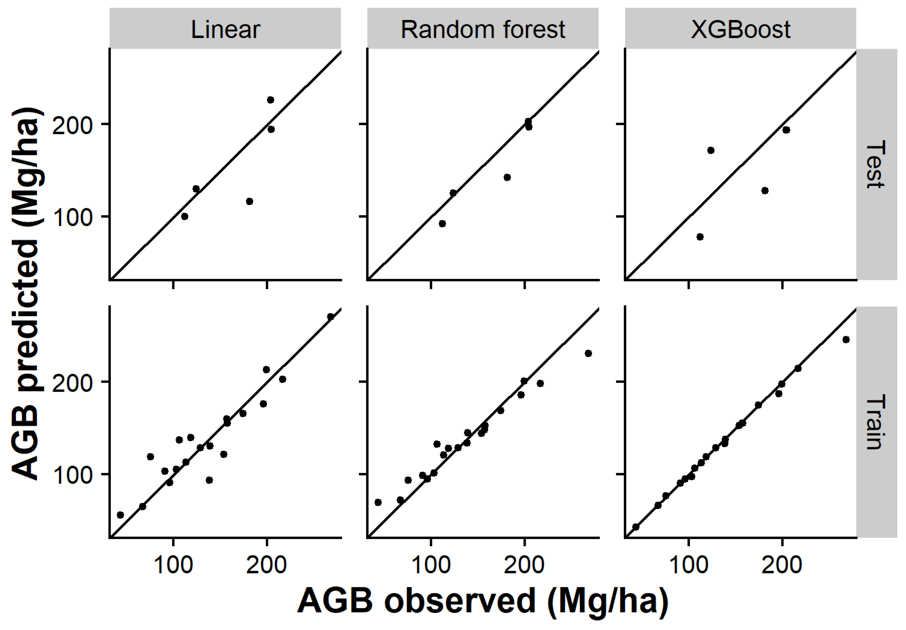
The AGB data of the mangrove and tropical swamp forest plots showed a mean AGB value of 142.8 Mg/ha and a standard deviation of 53.62 Mg/ha. Additionally, the data reveals a positive relation between the mean height and AGB. As the mean height increases, there is a noticeable increase in AGB, with the lowest AGB being 42.98 Mg/ha at a mean height of 8.19 m and the highest reaching 268.17 Mg/ha at a mean height of 16.6 m (Table S1).

The uncertainty of each plot’s AGB followed a general positive relation between the AGB uncertainty (i.e., sdAGB) and AGB mean values (Figure 3). This translates into plots with larger AGB also having more uncertainty. Overall, the highest AGB values are found in plots with mean heights exceeding 13 m, with the maximum AGB recorded at the highest mean height of 16.6 m (Figure 3).

3.2. Models

The model that achieved the lowest error on the test set was the random forest (RMSE = 20.24 Mg/ha, rRMSE = 12.25%, R² = 0.88, MAE = 14.25 Mg/ha, and MAPE = 9.19%), followed by the linear regression (RMSE = 31.80 Mg/ha, rRMSE = 19.24%, R² = 0.63, MAE = 23.34 Mg/ha, and MAPE = 13.63%) and XGBoost (RMSE = 36.22 Mg/ha, rRMSE = 21.91%, R² = 0.46, MAE = 31.46 Mg/ha, and MAPE = 21.83%) (

Table 1. Models that achieved the lowest RMSE on the test data for the random forest, XGBoost, and linear models.

Dataset	Model	Var 1	Var 2	Var 3	RMSE	rRMSE (%)	R2	MAE	MAPE
Training	Random forest	zmean	zq35	p4th	14.31	10.43	0.97	10.58	9.91
	XGBoost	zq55	p4th	zq95	5.80	4.23	0.99	2.94	1.76
	Linear	zmean	p5th	p2th	19.60	14.29	0.87	14.02	12.54
Test	Random forest	zmean	zq35	p4th	20.24	12.25	0.88	14.25	9.19
	XGBoost	zq55	p4th	zq95	36.22	21.91	0.46	31.46	21.83
	Linear	zmean	p5th	p2th	31.80	19.24	0.63	23.34	13.63

and Figure 4). All the models achieved a smaller error on the training set, while they differed mostly in their performance on the test set (Table 1 and Figure 4).

The variables incorporated in the final best model were zmean, zq35, and p4th, in order of relative importance (100, 93.75, and 73.67, respectively). On the other hand, the correlation analyses showed that the three variables included in the model with the lowest error showed a significant positive relation with the AGB (

Table 2. Correlation coefficients between the LiDAR metrics included in the model that achieved the lowest RMSE on the test set and AGB.

Var 1	Var 2	Variable Importance	Pearson Coeff	p
AGB	zmean	100	0.85	<0.001
AGB	zq35	93.7	0.87	<0.001
AGB	p4th	73.7	0.53	0.006

).

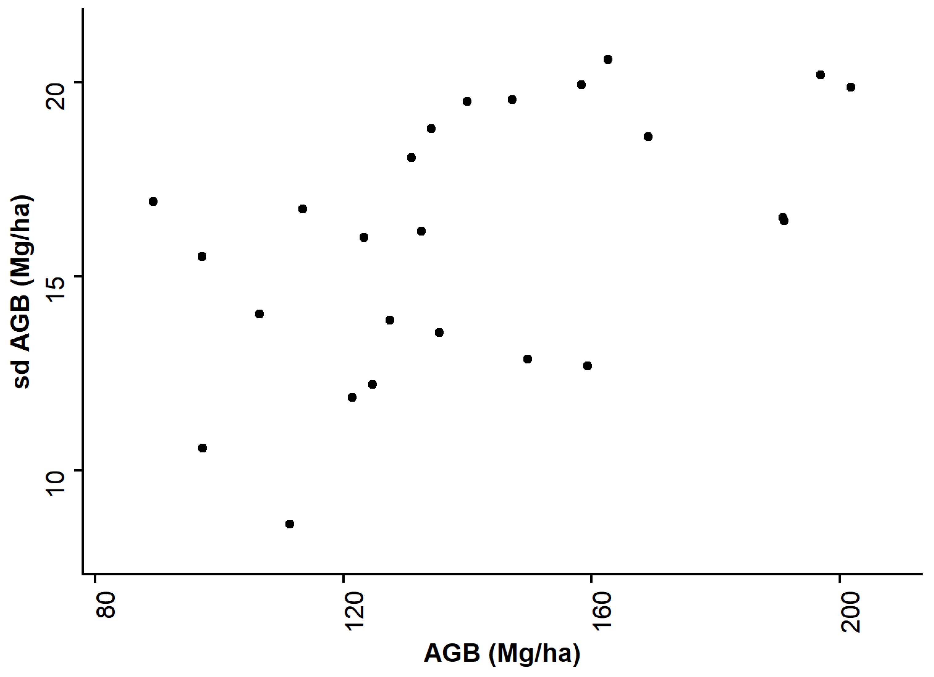
3.3. Uncertainty Analyses

The bootstrap analyses showed that the uncertainty in the complete gradient of observed AGB values was similar to the pattern shown in the per-plot AGB calculations (Figure 5). Therefore, a positive relationship was observed between the standard deviation and AGB values.

3.4. AGB Prediction for the Complete Study Area

The forested wetland’s AGB in the LiDAR footprint was a total of 96,096.71 ± 16,447.72 Mg, distributed across approximately 7.61 km² of forested wetlands. The spatial distribution of the AGB revealed elevated values along the secondary water channels of the lagoon and lower values towards the peripheries of the forest, particularly at the southwestern edge (Figure 6). The CoV indicated lower variability in regions with higher AGB and greater variability in areas with lower AGB. Despite this pattern, the overall variation across the entire study area was relatively small (i.e., less than 12%; Figure 6).

4. Discussion

This study demonstrates that LiDAR-derived metrics can effectively model AGB in mangroves and tropical swamp forests with a relatively small error (RMSE = 20.25 Mg/ha, rRMSE = 12.25%, R² = 0.88, MAE = 14.25 Mg/ha, and MAPE = 9.19%). Among the three modeling techniques evaluated—linear regression, random forest, and XGBoost—the random forest algorithm emerged as the most effective, outperforming both linear regression and XGBoost in terms of the observed error on the test set. The model with the lowest error included the zq35, zmean, and p4th metrics. Furthermore, the robustness of these predictions was confirmed through the randomization of both the training and test sets, as well as across the entire study area, indicating the model’s reliability and generalization in diverse conditions.

4.1. Models

Comparing the RMSE achieved on the training and test sets of the three best-performing models, it is evident the XGBoost overfitted on the training dataset, since it showed the lowest RMSE on the training set and the highest RMSE on the test set. In turn, the linear regression model underfitted on the training set but performed intermediately on the test set. Consequently, the random forest model represented a mid-point between the over- and underfitting of the other two models on the training set.

The linear models probably performed worse than the random forest ones due to their limited capacity to capture non-linear relationships between the LiDAR metrics and AGB. In contrast, machine learning techniques, such as random forest and XGBoost, are capable of working with non-parametric data and capturing non-linear interactions [73,74]. Nonetheless, due to the small sample size available in this study, the boosting mechanism in XGBoost caused an overfitting on the training data. Similar to previous reports, our study confirms that random forest is a robust modeling method capable of obtaining relatively low errors even when working with small sample sizes [48,50,52,53]. Future studies could benefit from using non-parametric modeling techniques to predict AGB based on LiDAR metrics [72].

The model that achieved the lowest RMSE included zmean, zq35, and p4th metrics. The first two variables are associated with the vertical structure of the forest, and no variable characterizing the intensity of the laser’s return was included. These findings agree with previous reports, since only vertical structure metrics were included in the best models [36,52,53].

Previous attempts to model AGB with LiDAR-derived metrics have reported that the maximum canopy height or quantiles above 90% are among the best height metrics for modeling AGB [32,35,36,49]. Our findings indicate that the model with the lowest RMSE did not include the total height (zmax); however, the mean height was highly correlated with the latter (zmean; r = 0.81). In fact, zmax was removed from the modeling process to avoid highly collinear variables. Although zmax was not tested in our models, it surely represents a variable with a high potential for predicting AGB. Thus, our results confirm the utility of LiDAR-derived percentile height metrics to model AGB, although not necessarily using single predictor models and the most frequent percentiles (i.e., max height) [31,32,35,36,46,49,52,53,69,70,71,72].

We infer that the positive relation between AGB and higher zq35 and zmean might be associated with communities characterized by higher and denser canopies. Previous studies have found similar results, in which taller stands usually contain larger carbon stocks [19,26,32,36,48,49,50]. In addition, we conjecture that the positive relation between AGB and the p4th variable is related to the canopy’s density. Since the studied forest has waterlogged areas, we hypothesize that forests with sparser canopies might have a lower percentage of fourth returns due to the absorption by water.

Compared to a previous attempt to model the same forest’s AGB using gray-level co-occurrence metrics (GLCM) texture metrics [43] from a very high-resolution multispectral image, the current study achieved a lower RMSE and higher R² (RMSE = 20.25 Mg/ha; R² = 0.88 vs. RMSE = 26.62 Mg/ha; R² = 0.65). This result underscores the greater potential of LiDAR-derived metrics in comparison with texture-derived from multispectral imagery.

In the context of previous reports, particular plots’ AGB correspond to some of the largest AGB values reported in mangroves or tropical swamp forests in Mexico, but most of the reported AGB values fall into the AGB range reported for the region [8,9,75,76,77,78,79]. The similarity in AGB estimates of these previous reports supports the accuracy of our AGB estimates. In turn, comparing these values with other forested wetlands worldwide, our AGB values fall in the smaller to intermediate AGB values [5,26,80]. Therefore, our AGB values are similar to other tropical swamp forests in Indonesia [48] and certain mangroves in Brazil [36,49], while smaller than certain tropical swamp forests of Indonesia and Brunei [19,50] and particular mangroves found in Gabon and Mozambique [32,81]. Thus, our AGB estimates in general align with worldwide AGB estimates for neotropical mangroves and forested wetlands in Mexico.

4.2. Spatial Patterns of AGB

Higher AGB values were concentrated in the areas closer to the main water channels (AGB ≥ 200 Mg/ha) and the southern part of the study area. These areas have an important presence of Rhizophora mangle, since these are commonly flooded and under higher salinity regimes, which coincides with previous reports of the relation of the inland presence of R. mangle with higher AGB values [22,79,82].

The total AGB in the forested cover of the study area (approximately 7.61 km²) was 96,096.71 ± 16,447.72 Mg, which represents a considerable carbon sink in the region. Certainly, the LiDAR point cloud did not cover the complete forest that surrounds El Cometa Lagoon or other forested areas in the region, but previous studies reported similar or slightly lower AGB values in other forested areas inside the biosphere reserve and the neighboring Laguna de Términos protected area [9,75,77]. Moreover, other authors reported enormous carbon stocks in the belowground component of the forest in Pantanos de Centla Biosphere Reserve and neighboring protected areas (i.e., Laguna de Términos), especially in the swamp forests and mixed forests [8,77]. Thus, the reserve represents large carbon reservoirs that should continue to be protected. Additionally, this information can be vital to promote the involvement of these areas as beneficiaries of programs such as payment for environmental services or carbon bonds.

4.3. Uncertainty Analyses

Several aspects contribute to the uncertainty in AGB estimation, including the size and shape of the plots, biomass model selection, scale differences between the plots and remote sensing data, date differences between the field sampling and LiDAR data, and field coordinates precision, among others [30,67,83,84]. Although all these aspects contribute to AGB uncertainty and interact among them, frequently, its effect can only be quantified for a few of them.

Since AGB uncertainty is calculated as a sum of the individual trees’ AGB, a larger uncertainty will usually be associated with plots with larger individuals or more trees. This exact pattern was observable in our results (Figure 3). Nonetheless, certain plots showed some deviation from this general pattern, which can be explained by either a higher presence of individuals with large DAP or height or species not identified to the species level. In the first case, it corresponds to particularly large individuals either in height or DAP that were present in the field, but no action can be performed to reduce the AGB uncertainty in these plots.

In the second case, previous studies have shown that including species identity for AGB calculation decreases the uncertainty in AGB values and errors associated with AGB modeling from LiDAR metrics [36,49]. Although we identified most individuals up to the species level, there were four morphospecies that we were unable to identify taxonomically. These species showed a higher uncertainty in their wood density values, since they were calculated from the identified species in the same plot. Although the occurrence of these species certainly increased the uncertainty in the AGB estimates, due to their rarity, their contribution to the AGB uncertainty was modest.

We assumed that the height metrics had no error in the Monte Carlo simulations, since they were directly measured in the field (although some previous studies have assumed a 0.5 m error [31]). This is obviously optimistic and unrealistic; however, there was no available field information to characterize this error. Although this aspect was not characterized in the field, we expect that the actual uncertainty in AGB values is slightly larger than the one presented here.

It is worth noting that, even though the size of our sampling plots could be regarded as small, based on previous studies [19,48,84,85], we were able to obtain predictions with relatively low uncertainty. This might be caused by the correspondence of scales between the LiDAR and field data [30] and the high precision used to capture the plots’ coordinates.

Furthermore, when analyzing the predictions made on the entire study area, the coefficient of variation values ranged from 0 to 12%, which shows relatively low uncertainty in the predictions made by the model (Figure 6). Interestingly, most of the uncertainty related to AGB predictions in the study area can be attributed to the field sampling uncertainty, since the one derived exclusively from the bootstrapped models corresponded only to 0–3% variation. This finding underscores the relevance of propagating AGB uncertainties into the AGB predictions, since it is very likely that overoptimistic error estimates can be obtained without including this process [30,31].

In the AGB prediction of the complete study area, a larger uncertainty can be associated with larger AGB values. This is a direct consequence of propagating the uncertainty obtained in the AGB calculation from field data into the modeling uncertainty. Without this propagation, the modeled AGB uncertainties did not show any particular pattern. Finally, the predictions of the model made on the observed AGB values range should be regarded as trustworthy, which agrees with previous findings [32,36,43].

4.4. Potential Limitations of the Study

Due to the relatively small sample size and study area, the generalization of our results to a larger area might lead to AGB estimations with larger uncertainty than the one shown in this study. Although we used a bootstrapping process to measure the variability of AGB predictions using different training data over the complete study area, admittedly, a more robust generalization could be obtained with a larger sample that covers a larger area [54,55]. Nonetheless, due to financial and time restrictions, it was impossible to achieve this. Future studies should prioritize data sharing to increase the available sample size, although its generalization might be still hindered by the lack of LiDAR data over large areas.

Seasonal variations can alter the information registered from LiDAR sensors, especially in deciduous communities or forests with dead individuals [70,71,86]. Since the forested wetland studied in this work consisted of a perennial community, the effects of seasonality on the LiDAR metrics should be small and should consist of variations caused by leaf growth/non-growth cycles [71,87]. Thus, we expect that our AGB estimates and LiDAR metrics could vary with the season of data acquisition; however, this variation should be small. Conversely, we expect that the highest seasonal variation could be expected in the LiDAR metrics in response to waterlogging conditions [88]. Since the LiDAR data were registered in the dry season, we expected less interference of water with the NIR laser; however, a higher water level could make the extraction of the DTM difficult and consequently, the vegetation normalization process. Therefore, LiDAR data acquisition in forested wetlands should be prioritized during the period with the lowest water level to facilitate forest height normalization.

We acknowledge that a 3-year time lag between the LiDAR data acquisition and the field data registration could have added noise to our models. Since the area corresponds to a protected area with a small presence of human activity (except fishing), no major disturbances were expected in this period. We confirmed this scenario by visually interpreting Sentinel-2 and Google Earth images. Better models could have been obtained with a smaller time gap between the LiDAR and field data acquisitions; however, due to financial issues, this was not possible.

Previous studies suggest that locally developed equations might be better for decreasing the error for calculating the AGB [89,90], while others suggest the opposite [91,92]. In addition, in other available allometric equations, other frequent companion species in our study, such as Pachira aquatica and Bucida buceras, were not included, neither in locally developed equations [93] nor global [22]. Thus, we chose the pantropical equation developed by [20] to calculate the AGB for each species using its corresponding wood-specific gravity. Nonetheless, we acknowledge that using different allometric models could potentially alter the AGB estimates by a relatively moderate magnitude.

4.5. Future Monitoring Proposals

The significance of this research extends beyond the immediate study area. As LiDAR technology becomes more widely available and its application in forested ecosystems continues to expand, the approach developed in this study could serve as scientific evidence to support AGB estimations in other mangroves or tropical swamp forests. Notably, Mexico, with its extensive forested wetland surface, stands out as a key area for applying these methodologies [5,10,26].

Previous studies have reported that one of the best AGB predictors is the maximum canopy height [32,36,49]. Although this variable can be obtained using other remote sensing techniques (e.g., Interferometric Synthetic Aperture Radar (InSAR) [29,46]), the use of LiDAR has the advantage of providing other metrics that describe the 3D structure of the forest (e.g., height percentiles or percentages of xth returns). As in this study, future AGB monitoring proposals could decrease the error in AGB predictions by including other cloud metrics derived from LiDAR in its models and using models that include more than one predictor.

Since 2019, Global Ecosystem Dynamics Investigation (GEDI) has democratized the use of LiDAR data to monitor forests’ AGB over large extents, since it is the first LiDAR data with worldwide cover and free access [94]. Although this mission is a huge advance in the development of tools to monitor AGB using remote sensors, its acquisition nature can prevent overlapping with field-acquired data to produce wall-to-wall AGB predictions [35]. Although the current study did not use GEDI data, our results provide a valuable link between LiDAR and field data that could afterward be used as a link between LiDAR and GEDI data to inform future attempts to model AGB over larger areas. For example, the most effective model in this study included zq35 and zmean, two metrics that can easily be obtained from GEDI products. Therefore, future monitoring methods can build upon these results to model tropical wetlands’ AGB with GEDI data and ultimately combine them with other types of images (e.g., multispectral and SAR) to enable wall-to-wall AGB mapping [95,96,97,98,99].

5. Conclusions

This study underscores the efficacy of LiDAR-derived metrics in modeling AGB in mangroves and tropical swamp forests, achieving a RMSE of 20.25 Mg/ha (rRMSE = 12.25%), with random forest emerging as the superior modeling technique. The model’s success was attributed to the inclusion of vertical structure metrics, such as zmean and zq35, which were significantly correlated with the AGB values. The findings highlight the robustness and reliability of the random forest models, even with the constraints of a relatively small sample size. Compared to other methods, including linear regression and XGBoost, random forest demonstrated a balanced performance between overfitting and underfitting, validating its effectiveness in handling LiDAR data for biomass estimations. Moreover, the study reveals that the spatial distribution of AGB correlates closely with the forest’s proximity to water channels and its vertical structure, affirming the importance of canopy metrics in biomass modeling. While the analysis acknowledged limitations related to sample size, the model’s predictions remained relatively robust. This research contributes valuable insights into the application of LiDAR technology for AGB estimations and emphasizes the potential for scaling such methodologies using additional remote sensing tools. Future research should explore integrating SAR and multispectral data to further enhance AGB modeling and leverage freely available datasets like GEDI to extend these techniques to broader areas.

References

1. Donato, D.; Kauffman, J.B.; Murdiyarso, D.; Kurnianto, S.; Stidham, M.; Kanninen, M. Mangroves Among the Most Carbon-Rich Forests in the Tropics. Nat. Geosci. 2011, 4, 293–297. [Google Scholar] [CrossRef]
2. Alongi, D.M. Carbon Cycling and Storage in Mangrove Forests. Annu. Rev. Mar. Sci. 2014, 6, 195–219. [Google Scholar] [CrossRef] [PubMed]
3. Lugo, A.E.; Brown, S.; Brinson, M. Ecosystems of the World, 15. Forested Wetlands; Elsevier Science Publishers: Amsterdam, The Netherlands, 1990; Volume 2, p. 527. ISBN 0444428127. [Google Scholar]
4. Ainslie, W.B. Forested Wetlands. In Southern Forest Resource Assessment; Wear, D.N., Greis, J.G., Eds.; General Technical Report; U.S. Department of Agriculture, Forest Service: Washington, DC, USA, 2002; pp. 479–499. [Google Scholar]
5. Hutchison, J.; Manica, A.; Swetnam, R.; Balmford, A.; Spalding, M. Predicting Global Patterns in Mangrove Forest Biomass. Conserv. Lett. 2014, 7, 233–240. [Google Scholar] [CrossRef]
6. FAO. The World’s Mangroves 2000–2020; FAO: Rome, Italy, 2023. [Google Scholar]
7. Murdiyarso, D.; Purbopuspito, J.; Kauffman, J.B.; Warren, M.W.; Sasmito, S.D.; Donato, D.C.; Manuri, S.; Krisnawati, H.; Taberima, S.; Kurnianto, S. The Potential of Indonesian Mangrove Forests for Global Climate Change Mitigation. Nat. Clim. Change 2015, 5, 1089–1092. [Google Scholar] [CrossRef]
8. Sjögersten, S.; Barreda-Bautista, B.d.l.; Brown, C.; Boyd, D.; Lopez-Rosas, H.; Hernandez, M.E.; Monroy, R.; Rincon, M.; Vane, C.; Moss-Hayes, V.; et al. Coastal Wetland Ecosystems Deliver Large Carbon Stocks in Tropical Mexico. Geoderma 2021, 403, 115173. [Google Scholar] [CrossRef]
9. Kauffman, J.B.; Trejo, H.H.; Carmen Jesus Garcia, M.d.; Heider, C.; Contreras, W.M. Carbon Stocks of Mangroves and Losses Arising from Their Conversion to Cattle Pastures in the Pantanos de Centla, Mexico. Wetl. Ecol. Manag. 2016, 24, 203–216. [Google Scholar] [CrossRef]
10. Giri, C. Chandra Observation and Monitoring of Mangrove Forests Using Remote Sensing: Opportunities and Challenges. Remote Sens. 2016, 8, 783. [Google Scholar] [CrossRef]
11. Gao, G.; Beardall, J.; Jin, P.; Gao, L.; Xie, S.; Gao, K. A Review of Existing and Potential Blue Carbon Contributions to Climate Change Mitigation in the Anthropocene. J. Appl. Ecol. 2022, 59, 1686–1699. [Google Scholar] [CrossRef]
12. Ribeiro, K.; Pacheco, F.S.; Ferreira, J.W.; Sousa-Neto, E.R.d.; Hastie, A.; Krieger Filho, G.C.; Alvalá, P.C.; Forti, M.C.; Ometto, J.P. Tropical Peatlands and Their Contribution to the Global Carbon Cycle and Climate Change. Glob. Change Biol. 2021, 27, 489–505. [Google Scholar] [CrossRef]
13. Hilmi, N.; Chami, R.; Sutherland, M.D.; Hall-Spencer, J.M.; Lebleu, L.; Benitez, M.B.; Levin, L.A. The Role of Blue Carbon in Climate Change Mitigation and Carbon Stock Conservation. Front. Clim. 2021, 3, 710546. [Google Scholar] [CrossRef]
14. Larrazábal, A.; McCall, M.K.; Mwampamba, T.H.; Skutsch, M. The Role of Community Carbon Monitoring for REDD+: A Review of Experiences. Curr. Opin. Environ. Sustain. 2012, 4, 707–716. [Google Scholar] [CrossRef]
15. Theilade, I.; Rutishauser, E.; Poulsen, M.K. Community Assessment of Tropical Tree Biomass: Challenges and Opportunities for REDD+. Carbon Balance Manag. 2015, 10, 17. [Google Scholar] [CrossRef] [PubMed]
16. Tokola, T. Remote Sensing Concepts and Their Applicability in REDD+ Monitoring. Curr. For. Rep. 2015, 1, 252–260. [Google Scholar] [CrossRef]
17. Choudhary, B.; Dhar, V.; Pawase, A.S. Blue Carbon and the Role of Mangroves in Carbon Sequestration: Its Mechanisms, Estimation, Human Impacts and Conservation Strategies for Economic Incentives. J. Sea Res. 2024, 199, 102504. [Google Scholar] [CrossRef]
18. Rahman; Lokollo, F.F.; Manuputty, G.D.; Hukubun, R.D.; Krisye; Maryono; Wawo, M.; Wardiatno, Y. A Review on the Biodiversity and Conservation of Mangrove Ecosystems in Indonesia. Biodivers. Conserv. 2024, 33, 875–903. [Google Scholar] [CrossRef]
19. Manuri, S.; Andersen, H.-E.; McGaughey, R.J.; Brack, C. Assessing the Influence of Return Density on Estimation of Lidar-Based Aboveground Biomass in Tropical Peat Swamp Forests of Kalimantan, Indonesia. Int. J. Appl. Earth Obs. Geoinf. 2017, 56, 24–35. [Google Scholar] [CrossRef]
20. Chave, J.; Réjou-Méchain, M.; Búrquez, A.; Chidumayo, E.; Colgan, M.S.; Delitti, W.B.C.; Duque, A.; Eid, T.; Fearnside, P.M.; Goodman, R.C.; et al. Improved Allometric Models to Estimate the Aboveground Biomass of Tropical Trees. Glob. Change Biol. 2014, 20, 3177–3190. [Google Scholar] [CrossRef]
21. Feldpausch, T.R.; Banin, L.; Phillips, O.L.; Baker, T.R.; Lewis, S.L.; Quesada, C.A.; Affum-Baffoe, K.; Arets, E.J.M.M.; Berry, N.J.; Bird, M.; et al. Height-Diameter Allometry of Tropical Forest Trees. Biogeosciences 2011, 8, 1081–1106. [Google Scholar] [CrossRef]
22. Komiyama, A.; Ong, J.E.; Poungparn, S. Allometry, Biomass, and Productivity of Mangrove Forests: A Review. Aquat. Bot. 2008, 89, 128–137. [Google Scholar] [CrossRef]
23. Vorster, A.G.; Evangelista, P.H.; Stovall, A.E.L.; Ex, S. Variability and Uncertainty in Forest Biomass Estimates from the Tree to Landscape Scale: The Role of Allometric Equations. Carbon Balance Manag. 2020, 15, 8. [Google Scholar] [CrossRef]
24. Kuenzer, C.; Bluemel, A.; Gebhardt, S.; Quoc, T.V.; Dech, S. Remote Sensing of Mangrove Ecosystems: A Review. Remote Sens. 2011, 3, 878–928. [Google Scholar] [CrossRef]
25. Lu, D.; Chen, Q.; Wang, G.; Liu, L.; Li, G.; Moran, E. A Survey of Remote Sensing-Based Aboveground Biomass Estimation Methods in Forest Ecosystems. Int. J. Digit. Earth 2016, 9, 63–105. [Google Scholar] [CrossRef]
26. Simard, M.; Fatoyinbo, L.; Smetanka, C.; Rivera-Monroy, V.H.; Castañeda-Moya, E.; Thomas, N.; Van der Stocken, T. Mangrove Canopy Height Globally Related to Precipitation, Temperature and Cyclone Frequency. Nat. Geosci. 2019, 12, 40–45. [Google Scholar] [CrossRef]
27. Saatchi, S. SAR Methods for Mapping and Monitoring Forest Biomass. In The Synthetic Aperture Radar (SAR) Handbook: Comprehensive Methodologies for Forest Monitoring and Biomass Estimation; Flores-Anderson, A.I., Herndon, K.E., Thapa, R.B., Cherrington, E., Eds.; NASA: Washington, DC, USA, 2019; pp. 207–247. [Google Scholar]
28. Feyisa, S.; Soromessa, T.; Bekele, T.; Bereta, A.; Hailemariam, F. Above Ground Biomass Estimation Methods and Challenges: A Review. Int. J. Energy Technol. Policy 2020, 9, 12–25. [Google Scholar] [CrossRef]
29. Singh, A.; Mahajan, S. A Review of SAR Image Processing for Mangrove Above Ground Biomass Estimation. J. Plant Sci. Res. 2023, 38, 779–789. [Google Scholar] [CrossRef]
30. Réjou-Méchain, M.; Barbier, N.; Couteron, P.; Ploton, P.; Vincent, G.; Herold, M.; Mermoz, S.; Saatchi, S.; Chave, J.; de Boissieu, F.; et al. Upscaling Forest Biomass from Field to Satellite Measurements: Sources of Errors and Ways to Reduce Them. Surv. Geophys. 2019, 40, 881–911. [Google Scholar] [CrossRef]
31. Rodda, S.R.; Fararoda, R.; Gopalakrishnan, R.; Jha, N.; Réjou-Méchain, M.; Couteron, P.; Barbier, N.; Alfonso, A.; Bako, O.; Bassama, P.; et al. LiDAR-Based Reference Aboveground Biomass Maps for Tropical Forests of South Asia and Central Africa. Sci. Data 2024, 11, 334. [Google Scholar] [CrossRef]
32. Fatoyinbo, T.; Feliciano, E.A.; Lagomasino, D.; Lee, S.K.; Trettin, C. Estimating Mangrove Aboveground Biomass from Airborne LiDAR Data: A Case Study from the Zambezi River Delta. Environ. Res. Lett. 2018, 13, 025012. [Google Scholar] [CrossRef]
33. Stovall, A.E.L.; Fatoyinbo, T.; Thomas, N.M.; Armston, J.; Ebanega, M.O.; Simard, M.; Trettin, C.; Zogo, R.V.O.; Aken, I.A.; Debina, M.; et al. Comprehensive Comparison of Airborne and Spaceborne SAR and LiDAR Estimates of Forest Structure in the Tallest Mangrove Forest on Earth. Sci. Remote Sens. 2021, 4, 100034. [Google Scholar] [CrossRef]
34. Hernández-Stefanoni, J.L.; Castillo-Santiago, M.Á.; Mas, J.F.; Wheeler, C.E.; Andres-Mauricio, J.; Tun-Dzul, F.; George-Chacón, S.P.; Reyes-Palomeque, G.; Castellanos-Basto, B.; Vaca, R.; et al. Improving Aboveground Biomass Maps of Tropical Dry Forests by Integrating LiDAR, ALOS PALSAR, Climate and Field Data. Carbon Balance Manag. 2020, 15, 15. [Google Scholar] [CrossRef]
35. Duncanson, L.; Kellner, J.R.; Armston, J.; Dubayah, R.; Minor, D.M.; Hancock, S.; Healey, S.P.; Patterson, P.L.; Saarela, S.; Marselis, S.; et al. Aboveground Biomass Density Models for NASA’s Global Ecosystem Dynamics Investigation (GEDI) Lidar Mission. Remote Sens. Environ. 2022, 270, 112845. [Google Scholar] [CrossRef]
36. Souza Pereira, F.R.d.; Kampel, M.; Soares, M.L.G.; Estrada, G.C.D.; Bentz, C.; Vincent, G. Reducing Uncertainty in Mapping of Mangrove Aboveground Biomass Using Airborne Discrete Return Lidar Data. Remote Sens. 2018, 10, 637. [Google Scholar] [CrossRef]
37. Heumann, B.W. Satellite Remote Sensing of Mangrove Forests: Recent Advances and Future Opportunities. Prog. Phys. Geogr. 2011, 35, 87–108. [Google Scholar] [CrossRef]
38. Luo, S.; Wang, C.; Xi, X.; Nie, S.; Fan, X.; Chen, H.; Ma, D.; Liu, J.; Zou, J.; Lin, Y.; et al. Estimating Forest Aboveground Biomass Using Small-Footprint Full-Waveform Airborne LiDAR Data. Int. J. Appl. Earth Obs. Geoinf. 2019, 83, 101922. [Google Scholar] [CrossRef]
39. Garcia, M.; Saatchi, S.; Ferraz, A.; Silva, C.A.; Ustin, S.; Koltunov, A.; Balzter, H. Impact of Data Model and Point Density on Aboveground Forest Biomass Estimation from Airborne LiDAR. Carbon Balance Manag. 2017, 12, 4. [Google Scholar] [CrossRef] [PubMed]
40. Zaki, N.A.M.; Latif, Z.A. Carbon Sinks and Tropical Forest Biomass Estimation: A Review on Role of Remote Sensing in Aboveground-Biomass Modelling. Geocarto Int. 2017, 32, 701–716. [Google Scholar] [CrossRef]
41. Abbas, S.; Wong, M.S.; Wu, J.; Shahzad, N.; Irteza, S.M. Approaches of Satellite Remote Sensing for the Assessment of Above-Ground Biomass Across Tropical Forests: Pan-Tropical to National Scales. Remote Sens. 2020, 12, 3351. [Google Scholar] [CrossRef]
42. Tran, T.V.; Reef, R.; Zhu, X. A Review of Spectral Indices for Mangrove Remote Sensing. Remote Sens. 2022, 14, 4868. [Google Scholar] [CrossRef]
43. Solórzano, J.V.; Gallardo-Cruz, J.A.; González, E.J.; Peralta-Carreta, C.; Hernández-Gómez, M.; Oca, A.F.-M.d.; Cervantes-Jiménez, L.G. Contrasting the Potential of Fourier Transformed Ordination and Gray Level Co-Occurrence Matrix Textures to Model a Tropical Swamp Forest’s Structural and Diversity Attributes. J. Appl. Remote Sens. 2018, 12, 036006. [Google Scholar] [CrossRef]
44. Bastin, J.-F.F.; Barbier, N.; Couteron, P.; Adams, B.; Shapiro, A.; Bogaert, J.; Cannière, C.D. Aboveground Biomass Mapping of African Forest Mosaics Using Canopy Texture Analysis: Towards a Regional Approach. Ecol. Appl. 2014, 24, 1984–2001. [Google Scholar] [CrossRef]
45. Ballhorn, U.; Jubanski, J.; Kronseder, K.; Siegert, F. Airborne LiDAR Measurements to Estimate Tropical Peat Swamp Forest Above Ground Biomass. In Proceedings of the 2012 IEEE International Geoscience and Remote Sensing Symposium, Munich, Germany, 22–27 July 2012; pp. 1660–1663. [Google Scholar]
46. Schlund, M.; Erasmi, S.; Scipal, K. Comparison of Aboveground Biomass Estimation from InSAR and LiDAR Canopy Height Models in Tropical Forests. IEEE Geo-Sci. Remote Sens. Lett. 2020, 17, 367–371. [Google Scholar] [CrossRef]
47. Kumar, L.; Mutanga, O. Remote Sensing of Above-Ground Biomass. Remote Sens. 2017, 9, 935. [Google Scholar] [CrossRef]
48. Englhart, S.; Jubanski, J.; Siegert, F. Quantifying Dynamics in Tropical Peat Swamp Forest Biomass with Multi-Temporal LiDAR Datasets. Remote Sens. 2013, 5, 2368–2388. [Google Scholar] [CrossRef]
49. Salum, R.B.; Souza-Filho, P.W.M.; Simard, M.; Silva, C.A.; Fernandes, M.E.B.; Cougo, M.F.; Nascimento, W.d.; Rogers, K. Improving Mangrove Above-Ground Biomass Estimates Using LiDAR. Estuar. Coast. Shelf Sci. 2020, 236, 106585. [Google Scholar] [CrossRef]
50. Zadbagher, E.; Marangoz, A.M.; Becek, K. Estimation of Above-Ground Biomass Using Machine Learning Approaches with InSAR and LiDAR Data in Tropical Peat Swamp Forest of Brunei Darussalam. IForest 2024, 17, 172–179. [Google Scholar] [CrossRef]
51. Lary, D.J.; Alavi, A.H.; Gandomi, A.H.; Walker, A.L. Machine Learning in Geosciences and Remote Sensing. Geosci. Front. 2016, 7, 3–10. [Google Scholar] [CrossRef]
52. Johnson, L.K.; Mahoney, M.J.; Bevilacqua, E.; Stehman, S.V.; Domke, G.M.; Beier, C.M. Fine-Resolution Landscape-Scale Biomass Mapping Using a Spatiotemporal Patchwork of LiDAR Coverages. Int. J. Appl. Earth Obs. Geoinf. 2022, 114, 103059. [Google Scholar] [CrossRef]
53. Tian, Y.; Zhang, Q.; Huang, H.; Huang, Y.; Tao, J.; Zhou, G.; Zhang, Y.; Yang, Y.; Lin, J. Aboveground Biomass of Typical Invasive Mangroves and Its Distribution Patterns Using UAV-LiDAR Data in a Subtropical Estuary: Maoling River Estuary, Guangxi, China. Ecol. Indic. 2022, 136, 108694. [Google Scholar] [CrossRef]
54. Chen, M.; Qiu, X.; Zeng, W.; Peng, D. Combining Sample Plot Stratification and Machine Learning Algorithms to Improve Forest Aboveground Carbon Density Estimation in Northeast China Using Airborne LiDAR Data. Remote Sens. 2022, 14, 1477. [Google Scholar] [CrossRef]
55. Schuh, M.S.; Favarin, J.A.S.; Marchesan, J.; Alba, E.; Berra, E.F.; Pereira, R.S. Machine Learning and Generalized Linear Model Techniques to Predict Aboveground Biomass in Amazon Rainforest Using LiDAR Data. J. Appl. Remote Sens. 2020, 14, 034518. [Google Scholar] [CrossRef]
56. Rajput, D.; Wang, W.J.; Chen, C.C. Evaluation of a Decided Sample Size in Machine Learning Applications. BMC Bioinform. 2023, 24, 48. [Google Scholar] [CrossRef] [PubMed]
57. R Core Team. R: A Language and Environment for Statistical Computing; R Foundation for Statistical Computing: Vienna, Austria, 2024. [Google Scholar]
58. Réjou-Méchain, M.; Tanguy, A.; Piponiot, C.; Chave, J.; Hérault, B. Biomass: An r Package for Estimating Above-Ground Biomass and Its Uncertainty in Tropical Forests. Methods Ecol. Evol. 2017, 8, 1163–1167. [Google Scholar] [CrossRef]
59. Roussel, J.-R.; Auty, D.; Coops, N.C.; Tompalski, P.; Goodbody, T.R.H.; Meador, A.S.; Bourdon, J.-F.; de Boissieu, F.; Achim, A. lidR: An r Package for Analysis of Airborne Laser Scanning (ALS) Data. Remote Sens. Environ. 2020, 251, 112061. [Google Scholar] [CrossRef]
60. Kuhn, M.; Wickham, H. Tidymodels: A Collection of Packages for Modeling and Machine Learning Using Tidyverse Principles. 2020. Available online: https://cran.r-project.org/web/packages/tidymodels/index.html (accessed on 10 March 2025).
61. Liaw, A.; Wiener, M. Classification and Regression by randomForest. R News 2002, 2, 18–22. [Google Scholar]
62. Chen, T.; He, T.; Benesty, M.; Khotilovich, V.; Tang, Y.; Cho, H.; Chen, K.; Mitchell, R.; Cano, I.; Zhou, T.; et al. Xgboost: Extreme Gradient Boosting. 2024. Available online: https://cran.r-project.org/web/packages/xgboost/index.html (accessed on 10 March 2025).
63. Kuhn, M.; Vaughan, D.; Hvitfeldt, E. Yardstick: Tidy Characterizations of Model Performance. 2024. Available online: https://cran.r-project.org/web/packages/yardstick/index.html (accessed on 10 March 2025).
64. Dancho, M. Modeltime: The Tidymodels Extension for Time Series Modeling. 2024. Available online: https://cran.r-project.org/web/packages/modeltime/index.html (accessed on 10 March 2025).
65. Solórzano, J.V.; Gallardo-Cruz, J.A.; Peralta-Carreta, C.; Martínez-Camilo, R.; Oca, A.F.-M. de Plant Community Composition Patterns in Relation to Microtopography and Distance to Water Bodies in a Tropical Forested Wetland. Aquat. Bot. 2020, 167, 103295. [Google Scholar] [CrossRef]
66. Zanne, A.E.; Lopez-Gonzalez, G.; Coomes, D.A.; Ilic, J.; Jansen, S.; Lewis, S.L.; Miller, R.B.; Swenson, N.G.; Wiemann, M.C.; Chave, J. Towards a Worldwide Wood Economics Spectrum. Ecol. Lett. 2009, 12, 351–366. [Google Scholar] [CrossRef]
67. Chave, J.; Condit, R.; Aguilar, S.; Hernandez, A.; Lao, S.; Perez, R. Error Propagation and Scaling for Tropical Forest Biomass Estimates. Philosophical transactions of the Royal Society of London. Ser. B Biol. Sci. 2004, 359, 409–420. [Google Scholar] [CrossRef]
68. Woods, M.; Lim, K.; Treitz, P. Predicting Forest Stand Variables from LiDAR Data in the Great Lakes—St. Lawrence Forest of Ontario. For. Chron. 2008, 84, 827–839. [Google Scholar] [CrossRef]
69. Ma, J.; Zhang, W.; Ji, Y.; Huang, J.; Huang, G.; Wang, L. Total and Component Forest Aboveground Biomass Inversion via LiDAR-Derived Features and Machine Learning Algorithms. Front. Plant Sci. 2023, 14, 1258521. [Google Scholar] [CrossRef]
70. Salas, E.A.L. Waveform LiDAR Concepts and Applications for Potential Vegetation Phenology Monitoring and Modeling: A Comprehensive Review. Geo-Spat. Inf. Sci. 2021, 24, 179–200. [Google Scholar] [CrossRef]
71. Cushman, K.C.; Armston, J.; Dubayah, R.; Duncanson, L.; Hancock, S.; Janík, D.; Král, K.; Krůček, M.; Minor, D.M.; Tang, H.; et al. Impact of Leaf Phenology on Estimates of Aboveground Biomass Density in a Deciduous Broadleaf Forest from Simulated GEDI Lidar. Environ. Res. Lett. 2023, 18, 065009. [Google Scholar] [CrossRef]
72. Borsah, A.A.; Nazeer, M.; Wong, M.S. LIDAR-Based Forest Biomass Remote Sensing: A Review of Metrics, Methods, and Assessment Criteria for the Selection of Allometric Equations. Forests 2023, 14, 2095. [Google Scholar] [CrossRef]
73. Chen, T.; Guestrin, C. XGBoost: A Scalable Tree Boosting System. In Proceedings of the 22nd ACM SIGKDD International Conference on Knowledge Discovery and Data Mining, ACM, San Francisco, CA, USA, 13–17 August 2016. [Google Scholar]
74. Breiman, L. Random Forests. Mach. Learn. 2001, 45, 5–32. [Google Scholar] [CrossRef]
75. Korpela, I.; Polvivaara, A.; Hovi, A.; Junttila, S.; Holopainen, M. Influence of Phenology on Waveform Features in Deciduous and Coniferous Trees in Airborne LiDAR. Remote Sens. Environ. 2023, 293, 113618. [Google Scholar] [CrossRef]
76. Simonson, W.; Allen, H.; Coomes, D. Effect of Tree Phenology on Lidar Measurement of Mediterranean Forest Structure. Remote Sens. 2018, 10, 659. [Google Scholar] [CrossRef]
77. Shan, J.; Toth, C.K. Topographic Laser Ranging and Scanning: Principles and Processing; CRC Press: Boca Raton, FL, USA, 2018. [Google Scholar]
78. Guerra-Santos, J.J.; Cerón-Bretón, R.M.; Cerón-Bretón, J.G.; Damián-Hernández, D.L.; Sánchez-Junco, R.C.; Carmen Guevara Carrió, E. del Estimation of the Carbon Pool in Soil and Above-Ground Biomass Within Mangrove Forests in Southeast Mexico Using Allometric Equations. J. For. Res. 2014, 25, 129–134. [Google Scholar] [CrossRef]
79. Adame, M.F.; Gamboa, J.N.; Torres, O.; Kauffman, J.B.; Reza, M.; Caamal, J.P.; Herrera-Silveira, J.A.; Medina, I. Carbon Stocks of Tropical Coastal Wetlands Within the Karstic Landscape of the Mexican Caribbean. PLoS ONE 2013, 8, e56569. [Google Scholar] [CrossRef]
80. Troche-Souza, C.; Priego-Santander, A.; Equihua, J.; Vázquez-Balderas, B. Spatial Distribution of Carbon Stocks Along Protected and Non-Protected Coastal Wetland Ecosystems in the Gulf of Mexico. Ecosystems 2024, 72, 724–738. [Google Scholar] [CrossRef]
81. Ávila-Acosta, C.R.; Domínguez-Domínguez, M.; Vázquez-Navarrete, C.J.; Acosta-Pech, R.G.; Martínez-Zurimendi, P. Aboveground Biomass and Carbon Storage in Mangrove Forests in Southeastern Mexico. Resources 2024, 13, 41. [Google Scholar] [CrossRef]
82. Velázquez-Pérez, C.; Hernández, C.; Romero-Berny, E.; Jesús-Navarrete, A. Estructura del manglar y su influencia en el almacén de carbono en la Reserva La Encrucijada, Chiapas, México. Madera Bosques 2023, 25, e2531885. [Google Scholar] [CrossRef]
83. Giri, C.; Ochieng, E.; Tieszen, L.L.; Zhu, Z.; Singh, A.; Loveland, T.; Masek, J.; Duke, N.C. Status and Distribution of Mangrove Forests of the World Using Earth Observation Satellite Data. Glob. Ecol. Biogeogr. 2011, 20, 154–159. [Google Scholar] [CrossRef]
84. Trettin, C.C.; Dai, Z.; Tang, W.; Lagomasino, D.; Thomas, N.; Lee, S.K.; Simard, M.; Ebanega, M.O.; Stoval, A.; Fatoyinbo, T.E. Mangrove Carbon Stocks in Pongara National Park, Gabon. Estuar. Coast. Shelf Sci. 2021, 259, 107432. [Google Scholar] [CrossRef]
85. Rahman, M.S.; Donoghue, D.N.M.; Bracken, L.J.; Mahmood, H. Biomass Estimation in Mangrove Forests: A Comparison of Allometric Models Incorporating Species and Structural Information. Environ. Res. Lett. 2021, 16, 124002. [Google Scholar] [CrossRef]
86. Zhao, F.; Guo, Q.; Kelly, M. Allometric Equation Choice Impacts Lidar-Based Forest Biomass Estimates: A Case Study from the Sierra National Forest, CA. Agric. For. Meteorol. 2012, 165, 64–72. [Google Scholar] [CrossRef]
87. Price, C.A.; Branoff, B.; Cummins, K.; Kakaï, R.G.; Ogurcak, D.; Papeș, M.; Ross, M.; Whelan, K.R.T.; Schroeder, T.A. Global Data Compilation Across Climate Gradients Supports the Use of Common Allometric Equations for Three Transatlantic Mangrove Species. Ecol. Evol. 2024, 14, e70577. [Google Scholar] [CrossRef]
88. Rutishauser, E.; Noor’an, F.; Laumonier, Y.; Halperin, J.; Rufi’ie; Hergoualch, K.; Verchot, L. Generic Allometric Models Including Height Best Estimate Forest Biomass and Carbon Stocks in Indonesia. For. Ecol. Manag. 2013, 307, 219–225. [Google Scholar] [CrossRef]
89. Day, J.W.; Conner, W.H.; Ley-Lou, F.; Day, R.H.; Navarro, A.M. The Productivity and Composition of Mangrove Forests, Laguna de Términos, Mexico. Aquat. Bot. 1987, 27, 267–284. [Google Scholar] [CrossRef]
90. Chavez, S.; Wdowinski, S.; Lagomasino, D.; Castañeda-Moya, E.; Fatoyinbo, T.; Moyer, R.P.; Smoak, J.M. Estimating Structural Damage to Mangrove Forests Using Airborne Lidar Imagery: Case Study of Damage Induced by the 2017 Hurricane Irma to Mangroves in the Florida Everglades, USA. Sensors 2023, 23, 6669. [Google Scholar] [CrossRef]
91. Picard, N.; Bosela, F.B.; Rossi, V. Reducing the Error in Biomass Estimates Strongly Depends on Model Selection. Ann. For. Sci. 2015, 72, 811–823. [Google Scholar] [CrossRef]
92. Réjou-Méchain, M.; Muller-Landau, H.C.; Detto, M.; Thomas, S.C.; Toan, T.L.; Saatchi, S.S.; Barreto-Silva, J.S.; Bourg, N.A.; Bunyavejchewin, S.; Butt, N.; et al. Local Spatial Structure of Forest Biomass and Its Consequences for Remote Sensing of Carbon Stocks. Biogeosciences 2014, 11, 6827–6840. [Google Scholar] [CrossRef]
93. Hernández-Stefanoni, J.L.; Reyes-Palomeque, G.; Castillo-Santiago, M.Á.; George-Chacón, S.P.; Huechacona-Ruiz, A.H.; Tun-Dzul, F.; Rondon-Rivera, D.; Dupuy, J.M. Effects of Sample Plot Size and GPS Location Errors on Aboveground Biomass Estimates from LiDAR in Tropical Dry Forests. Remote Sens. 2018, 10, 1586. [Google Scholar] [CrossRef]
94. Dubayah, R.; Armston, J.; Healey, S.P.; Bruening, J.M.; Patterson, P.L.; Kellner, J.R.; Duncanson, L.; Saarela, S.; Ståhl, G.; Yang, Z.; et al. GEDI Launches a New Era of Biomass Inference from Space. Environ. Res. Lett. 2022, 17, 095001. [Google Scholar] [CrossRef]
95. Saarela, S.; Holm, S.; Healey, S.P.; Patterson, P.L.; Yang, Z.; Andersen, H.-E.; Dubayah, R.O.; Qi, W.; Duncanson, L.I.; Armston, J.D.; et al. Comparing Frameworks for Biomass Prediction for the Global Ecosystem Dynamics Investigation. Remote Sens. Environ. 2022, 278, 113074. [Google Scholar] [CrossRef]
96. Tommaso, S.D.; Wang, S.; Lobell, D.B. Combining GEDI and Sentinel-2 for Wall-to-Wall Mapping of Tall and Short Crops. Environ. Res. Lett. 2021, 16, 125002. [Google Scholar] [CrossRef]
97. Adrah, E.; Wong, J.P.; Yin, H. Integrating GEDI, Sentinel-2, and Sentinel-1 Imagery for Tree Crops Mapping. Remote Sens. Environ. 2025, 319, 114644. [Google Scholar] [CrossRef]
98. Doyog, N.D.; Lin, C. Generating Wall-to-Wall Canopy Height Information from Discrete Data Provided by Spaceborne LiDAR System. Forests 2024, 15, 482. [Google Scholar] [CrossRef]
99. Wang, C.; Elmore, A.J.; Numata, I.; Cochrane, M.A.; Lei, S.; Hakkenberg, C.R.; Li, Y.; Zhao, Y.; Tian, Y. A Framework for Improving Wall-to-Wall Canopy Height Mapping by Integrating GEDI LiDAR. Remote Sens. 2022, 14, 3618. [Google Scholar] [CrossRef]
Figure 1. Schematic representation of all the steps followed in the study.
Remotesensing 17 01076 g001
Figure 2. Location of the study site and sampled plots. In addition, a digital surface model (DSM) calculated from the LiDAR data is shown in grayscale.
Remotesensing 17 01076 g002
Figure 3. AGB and its uncertainty in the sampled plots.
Remotesensing 17 01076 g003
Figure 4. Comparisons among the fitted models on the training and test sets.
Remotesensing 17 01076 g004
Figure 5. Uncertainty of the AGB predictions made by the random forest trained and tested on the bootstrapped datasets.
Remotesensing 17 01076 g005
Figure 6. (a) Mean AGB prediction of the study area. (b) Coefficient of variation (CoV) of the AGB of the study area.
Remotesensing 17 01076 g006