Direct and Indirect Impacts of Urbanization on Biodiversity Across the World’s Cities

Abstract

Biodiversity has important implications for the sustainable development of cities. Given the paucity of ground-based experiments, the responses of biodiversity to urbanization and its associated controls on a global scale remain largely unexplored. We present a novel conceptual framework for quantifying the direct and indirect impacts of urbanization on biodiversity in 1523 cities worldwide using the global 100 m grid biodiversity intactness index data (2017–2020) as a proxy for biodiversity. The results show a pervasive positive impact of urbanization on biodiversity in global cities, with a global mean direct and indirect impact of 24.85 ± 9.97% and 16.18 ± 10.92%, respectively. The indirect impact is relatively large in highly urbanized cities in the eastern United States, Western Europe, and the Middle East. The indirect impact is predominantly influenced by urbanization intensity, population density, and background climate. The correlation between urbanization intensity and indirect impact is most pronounced across all climate zones, while the other driving variables influencing the indirect effect exhibited considerable variations. Furthermore, our findings indicate that the biodiversity responses to urbanization are influenced by the biodiversity and development conditions of cities. Our findings have important implications for understanding the impact of urbanization on biodiversity and for future sustainable urban biodiversity.

1. Introduction

Urbanization and its associated human activities have a profound impact on landscapes and local climates. This is evidenced by the transformation of natural vegetated surfaces to built-up areas, as well as changes in atmospheric and climatic conditions within the urban–biosphere system [1,2]. Urban environments are increasingly recognized as “harbingers” of future global climate change [3], offering unique opportunities to study biodiversity dynamics under compounded anthropogenic pressures. These environments serve as “natural laboratories” due to their heterogeneous microhabitats, intensified human–nature interactions, and accelerated environmental stressors (e.g., heat islands, pollution gradients, and habitat fragmentation). Together, these factors simulate predicted global change scenarios, providing controlled yet complex systems to observe phenotypic adaptations and species survival strategies under rapid environmental changes [4,5]. Consequently, a substantial body of literature has documented the implications of current and future urbanization on biodiversity over the past decades [6,7]. An investigation into the impact of urban environments on global biodiversity dynamics and the associated determinants has the potential to enhance our comprehension of biodiversity in response to future global changes [1,8].

Urbanization impacts biodiversity through direct habitat alteration and indirect cascading effects [1,9,10]. Direct impacts are primarily manifested in the occupation of physical space and structural damage to habitats [11,12]. The replacement of natural surfaces (e.g., forests and wetlands) with impermeable layers (e.g., buildings and roads) has been demonstrated to lead to habitat fragmentation and loss of connectivity, which directly result in a reduction in the range of species and, consequently, a significant reduction in the number of organisms [13,14,15]. For instance, a study conducted in the Lhasa River Basin in China revealed that urban expansion led to a decline in habitat quality, particularly in the farmland protection scenario, where the maximum decline reached 22.52% [16]. Furthermore, simulation experiments have demonstrated that sudden land changes also trigger long-term changes in species composition through the “extinction debt” mechanism and that biodiversity takes more than 10 years to recover [17].

Urbanization exerts an indirect influence on biodiversity through three synergistic pathways in natural-anthropogenic environments [18,19]. Firstly, alterations to climate regulation via the effects of urban heat islands disrupt species’ thermal tolerance and synchronization of activities, such as mismatches between plant flowering and pollinator activity [20,21]. Secondly, changes in soil moisture and compaction reduce mycorrhizal fungal diversity, which is critical for plant nutrient acquisition, and this, in turn, affects food chains [22]. Thirdly, anthropogenic stressors such as impermeable surfaces and artificial lighting impose novel hydrological and behavioral pressures, reshaping species adaptation and predator–prey dynamics [23,24]. These interconnected drivers amplify compounding stresses (e.g., warming-induced evapotranspiration exacerbating soil moisture deficits), exceeding the adaptive capacity of specialist species and restructuring communities through habitat suitability gradients [25,26].

Despite the fact that a significant number of studies have explored the impacts of urbanization on biodiversity, there are still some limitations. At present, the majority of research focuses on the direct effects of cities on biodiversity, with only a few studies quantifying the indirect impacts of urbanization on biodiversity and its potential controlling factors. In order to narrow this research gap, it is necessary to strengthen scientific studies on the indirect effects of urbanization on biodiversity, including the further development of assessment frameworks and methods [1]. Moreover, due to the paucity of extensive ground-based experiments, research on both the direct and indirect impacts of urbanization on biodiversity has mainly been conducted at local scales, resulting in a lack of comprehensive understanding at the global level. Given the aforementioned limitations, we combined globally acquirable 100 m grid biodiversity intactness index data, multi-source satellite imagery, and reanalysis data from 2017 to 2020 and examined the direct and indirect impacts of urbanization on biodiversity dynamics across 1523 cities worldwide based on a well-defined conceptual framework. Additionally, we explored the potential factors controlling the indirect impacts. The conceptual framework of this paper draws inspiration from a computational framework initially proposed by Zhao et al. [27], which was subsequently expanded by Zhang et al. [28] into a global investigation to quantify the direct and indirect impacts of urbanization on vegetation cover. Zhao et al.’s framework quantify the direct and indirect impacts of urbanization on vegetation growth by analyzing the difference between the theoretical linear decline of zero impact and the observed nonlinear decline of vegetation cover along the urban–rural gradient [27]. Given the established correlation between biodiversity and vegetation [29], Zhao et al.’s framework can also be applied to quantify the direct, indirect, and overall impacts of urbanization on biodiversity (for details, see Section 2.3). To the best of our knowledge, our results provide the first insight into the patterns and causes of the direct and indirect impacts of urbanization on biodiversity dynamics across global cities. These findings provide an enhanced interpretation of the impact of global urbanization on biodiversity dynamics, which can inform the development of more effective biodiversity conservation policies.

2. Materials and Methods

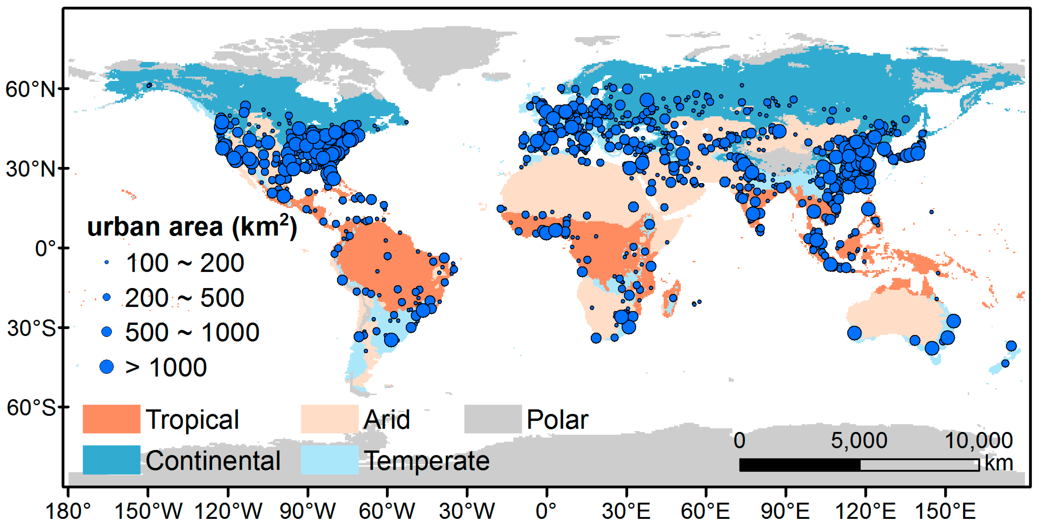
2.1. Study Area

A total of 1523 global city clusters (hereafter referred to as cities) with city sizes larger than 100 km² (Figure 1) were selected based on global urban boundary (GUB) data from 2018 [30]. Given that we used multi-source remote sensing data, it was necessary to ensure that each city contained a sufficient number of available remote sensing pixels for further calculations. Therefore, similar to global urban studies [28], we selected cities with an area greater than 100 km² for the analysis. The selected cities were situated within five distinct climatic zones, as defined by the updated Koppen–Geiger classification scheme [31], namely tropical, arid, temperate, continental, and polar.

2.2. Data

Biodiversity intactness index data. The biodiversity intactness index (BII) provides a quantitative measure of local community intactness within a given pixel or area [32]. It is frequently used as a proxy indicator to characterize biodiversity [33]. The BII values range from 0 to 100%. It provides a statistical analysis of the average community abundance of species that were originally present in a given area in comparison relative to their original abundance in an undisturbed habitat [32]. For example, a BII of 50% indicates that the species in an area are now half as common as they were in the past. The BII data were generated as 100 m gridded maps from 2017 to 2020 and are available for acquisition from a public information-sharing center (https://gee-community-catalog.org/projects/bii/, accessed on 22 July 2023). In this study, we employed BII data from 2017 to 2020 to evaluate the impact of urbanization on biodiversity at the global city level.

Urban boundary data. Cities with an urban area exceeding 100 km² were extracted from the GUB data of 2018 [30]. The GUB data has a spatial resolution of 30 m with long-term records from 1990 to 2018 with a 5-year interval. It can be accessed at a public information-sharing center (https://data-starcloud.pcl.ac.cn/zh, accessed on 29 July 2023). The GUB data provide an accurate global mapping of the urban boundaries of cities, which exhibits a high degree of correspondence with other similar urban boundary products. We used the GUB data from 2018, as they are the most proximate to the BII data utilized for the years 2017–2020.

Impervious surface percentage data. Annual maps of global impervious surface percentage (ISP) data from 2017 to 2018 were used to quantify the intensity of urbanization. The ISP data were generated at a 30 m resolution from 1985 to 2018 [34] and are available for download from a public data-sharing center (https://doi.org/10.5281/zenodo.4035352, accessed on 16 August 2023).

Climate data. A global map of the Köppen–Geiger climate classification was employed to delineate the five climate zones [31], including tropical, arid, temperate, continental, and polar. To obtain temperature and precipitation data for the cities, we employed the ERA5-Land monthly averaged data produced by the European Center for Medium-Range Weather Forecasts (https://cds.climate.copernicus.eu/datasets, accessed on 10 November 2023). The monthly mean air temperature at a 2 m height and monthly mean precipitation for each city were extracted from the ERA5-Land monthly averaged data for the period 2017 to 2020. The spatial resolution of the ERA5 air temperature and precipitation data is 0.01° (i.e., approximately 9 km).

Data about urban development. We used three datasets to characterize urban development in terms of population, economy, and urban green spaces. The human population data for each city were extracted from the LandScan datasets at the Oak Ridge National Laboratory (https://landscan.ornl.gov, accessed on 17 December 2023) for the period between 2017 and 2020. The spatial resolution of the human population data is 30 arcseconds (i.e., approximately 1 km). Economic growth is frequently regarded as a key indicator of urban development. Therefore, GDP data with a spatial resolution of 1 km from 2017 to 2020 were employed to capture urban development [35], which were obtained from a public data-sharing center (https://doi.org/10.6084/m9.figshare.17004523.v1, accessed on 20 August 2023). Urban green spaces are regarded as key indicators of human management of vegetation in cities [36]. The remotely sensed 16-day composite enhanced vegetation index (EVI) product (MOD13A1) with a spatial resolution of 500 m from 2017 to 2020 was used to characterize the spatial variability of vegetation cover and, consequently, urban greenspace in cities. Remotely sensed EVI data were obtained from the public data-sharing center operated by NASA (https://developers.google.com/earth-engine/datasets/catalog/MODIS_061_MYD13A1, accessed on 13 August 2023). It should be noted that all the data used were resampled to a spatial resolution of 100 m in order to match the spatial resolution of the BII data. Furthermore, both the ISP and EVI values range from 0 to 1. A higher ISP value indicates a greater built-up surface area (associated with urbanization intensity), whereas a higher EVI value indicates a greater vegetated surface area [28].

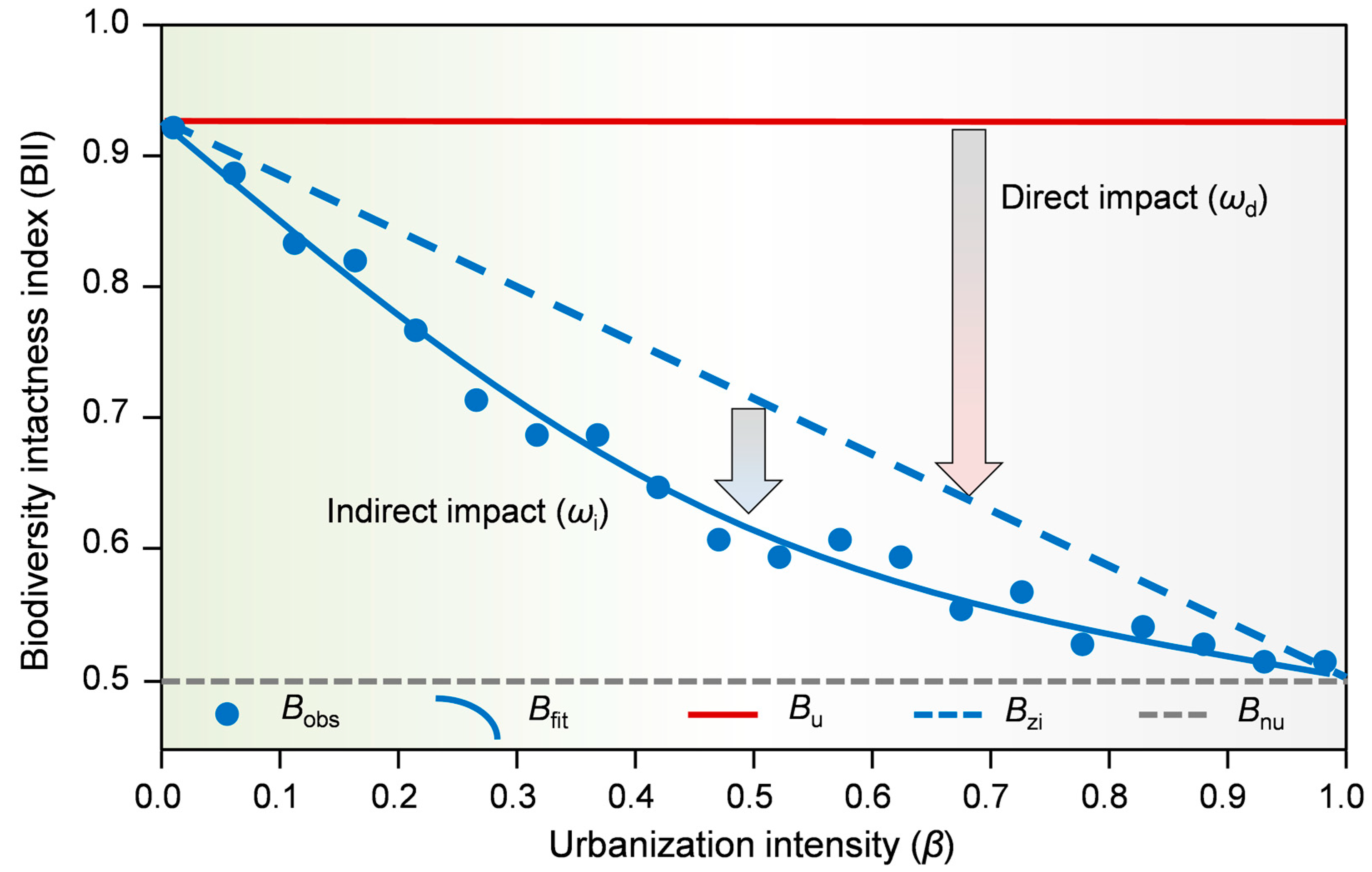
2.3. Quantification of the Direct and Indirect Impacts of Urbanization on Biodiversity

As previously stated, the urban areas of the 1523 cities selected for this study were extracted from the GUB data. A rural buffer zone (i.e., a rural area) extending outside each urban boundary was created to provide a comprehensive overview of the changes in biodiversity along the spatial gradient from urban to rural areas for each city. The rural area was established as a widely used buffer zone with a size equivalent to that of the urban area extending outward from the urban edge [28]. This approach avoids the disadvantage of adopting a fixed threshold for cities with different sizes.

This study draws upon the methodologies employed by Zhao et al. [27] and Zhang et al. [28] in analyzing the relationship between urbanization and vegetation growth. It assumes that when considering only the direct impact of urbanization, a linear relationship exists between the biodiversity integrity index (BII) and the intensity of urbanization (represented by the proportion of impervious surface ISP). This relationship is then utilized to construct a theoretical zero-impact line. The fundamental logic of this assumption is that if urbanization exerts its effect on biodiversity exclusively by directly replacing natural habitats, the BII should demonstrate a uniform downward trend with the increase of the ISP. Based on the baseline scenario provided by the zero-impact line, the conceptual framework for quantifying the direct, indirect, and total impacts of urbanization on biodiversity in this paper is shown in Figure 2.

The direct impact of urbanization on biodiversity (ω_d) refers to the change in biodiversity resulting from the replacement of natural habitats with urban areas within a city [1,10]. In general, biodiversity (represented by the BII) is observed to decrease with the increase in urbanization intensity (represented by the ISP corresponding to a BII pixel) along the spatial gradient from rural to urban areas. It can be reasonably assumed that a linear relationship between the BII and ISP will be observed when only the direct impact is considered (see dashed blue line in Figure 2). Accordingly, this linear BII–ISP relationship has also been regarded as a theoretical zero-impact line, which is expressed as follows:

$$B_{\mathrm{zi}}=(1-\beta )B_{\mathrm{u}}+\beta B_{\mathrm{nu}}$$

(1)

where B_zi represents the theoretical BII value of a pixel; β denotes the urbanization intensity, which is quantified by ISP values between 0 and 1; B_u signifies the mean BII of the pixels that are entirely covered by vegetated surfaces (β = 0), whereas B_nu denotes the mean BII of the pixels that are completely filled by built-up surfaces (β = 1). In order to mitigate the potential uncertainty, B_u and B_nu are calculated by the mean BII corresponding to an ISP less than 0.05 (see the dashed gray line in Figure 2) and greater than 0.95(see the solid red line in Figure 2), respectively, according to the 95% confidence intervals. Consequently, the direct impact of urbanization (ω_d) on biodiversity can be calculated as follows:

$${\omega }_{\mathrm{d}}={\displaystyle \frac{B_{\mathrm{zi}}-B_{\mathrm{u}}}{B_{\mathrm{u}}}}\times 100\%$$

(2)

When the actual observed BII values are in response to their corresponding gradient of urbanization intensity, it becomes evident that the observed BII may exhibit a nonlinear response curve to urbanization intensity and may not fully align with the theoretical zero-impact line (see the solid blue line in Figure 2). This indicates the presence of an indirect impact of urbanization on biodiversity. The indirect impact of urbanization (ω_i) refers to the difference between the observed BIIs (B_fit) and theoretical zero-impact line (B_zi), which is quantified using Equation (3). Consistent with previous studies [27,28], we employ the fitted observed BIIs rather than the actual observed BIIs to delineate the BII response curve to urbanization intensity in order to suppress the potential uncertainty induced by the natural variability of the data. Given that a cubic polynomial model can more effectively capture data with multi-stage variations compared to linear or quadratic polynomial models [27,28], this study employs a cubic polynomial model to fit the response curve of the BII to urbanization intensity (β) for each specific city (i.e., the BII~β curve), where x represents urbanization intensity (β) and y represents the observed BII.

$${\omega }_{\mathrm{i}}={\displaystyle \frac{B_{\mathrm{zi}}-B_{\mathrm{fit}}}{B_{\mathrm{zi}}}}\times 100\%$$

(3)

It is important to highlight that the indirect impact signifies an increase or decrease in biodiversity as a consequence of alterations to the urban environment caused by urbanization in comparison to the natural environment. The observation of a BII below the theoretical zero-impact line indicates a positive indirect impact, which is linked to the accelerated decrease in biodiversity resulting from alterations to the urban environment. Conversely, the observation of a BII above the theoretical zero-impact line denotes a negative indirect impact, which is associated with the compensatory increase in biodiversity caused by changes in the urban environment.

To characterize the BII variation along the gradient of urbanization intensity β, the mean BII value was calculated within each urbanization intensity β bin with an interval of 0.1 for each city. The mean ω_d and ω_i conditions for each city were calculated as the average of all ω_d and ω_i values across the range of urbanization intensities. The total realized urbanization impact (ω_t) was calculated as the sum of the ω_d and ω_i values. This study focuses on the spatial patterns and dominant determinants of the indirect impact of complex urban environments on biodiversity across global cities.

2.4. Analysis of Controlling Factors of the Indirect Impact on Biodiversity

To investigate the potential effects of climatic and anthropogenic factors on ω_i, six variables were selected as the potential climatic and anthropogenic factors. These included annual air temperature and precipitation, urbanization intensity, urban green space, and population density. Annual air temperatures and precipitation are well-documented indicators of background climatic conditions [37]. Annual air temperatures and precipitation data were retrieved from the atmospheric reanalysis product. Urbanization intensity was calculated using high-resolution ISP data. It is important to emphasize that the ISP data used here are not derived from theoretical models but from statistical analysis of real spatial data, independently reflecting the complex regulatory effects of the urban built environment on biodiversity. The urban green space serves as a crucial metric for assessing the impact of human intervention on natural vegetation within urban environments, with significant ramifications for biodiversity [38]. Consequently, the urban green space was determined as the mean of all EVI values within the urban area. The mean of all the pixel values for each potential driving factor from 2017 to 2020 within each city was calculated for subsequent analysis. A stepwise regression analysis was employed to ascertain the potential drivers that might control ω_i. Furthermore, the various patterns of ω_i between cities at different biodiversity and development levels were identified. The biodiversity and development levels were calculated as the mean BII and GDP within each urban area, respectively.

3. Results

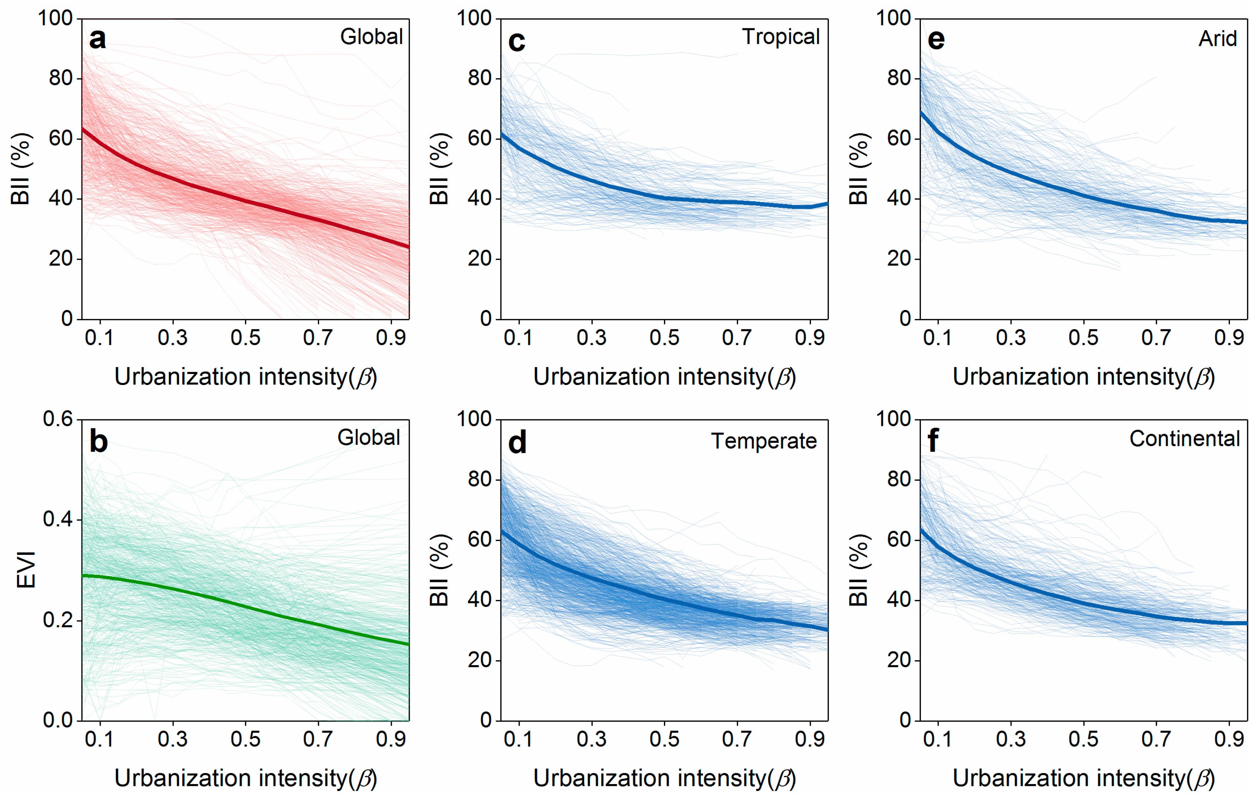
3.1. Direct and Indirect Urbanization Impacts on Biodiversity Dynamics

Across all cities, the BII decreases with increasing urbanization intensity (Figure 3a). This demonstrates the adverse direct impact of urbanization (ω_d) on biodiversity, whereby the coverage of biodiversity-based natural vegetated areas declines in tandem with the expansion of urban built-up areas (Figure 3b). Moreover, it is observed that the alterations in BII values in relation to urbanization intensity do not consistently align with the theoretical zero-impact line in most cases (Figure 3c–f). This can be attributed to the indirect impact of urbanization (ω_i) on biodiversity.

Overall, 1305 (86%) of the 1523 global cities show a positive ω_i. The global mean ω_i on biodiversity is 16.18 ± 10.92% (Figure 4a), characterized by a pattern of relatively larger ω_i in cities in the eastern United States, Western Europe, and the Middle East, and relatively smaller ω_d in most of Africa. A positive ω_d is observed across 1521 global cities, with a global mean ω_d of 24.85 ± 9.97% (Figure 4d). Cities in most of Europe, India, and eastern China had a relatively larger ω_d, whereas cities in the western United States and Russia revealed a relatively lower ω_d. Furthermore, it is observed that 1510 (99%) of the 1523 global cities exhibit a positive total impact of urbanization on biodiversity (ω_t), with a global average ω_t of 41.02 ± 16.07% (mean ± e standard deviation) (Figure S1). It is estimated that in 23% of the world’s cities, the ω_t is greater than 50%. Cities with a relatively higher ω_t are located in the eastern United States, Western Europe, the Middle East, and most of South America, whereas cities with a relatively lower ω_t occur in most of Africa and Oceania (Figure S1). Furthermore, minor variations in the ω_i are observed between different latitudes (Figure 4b), while insignificant latitudinal variations are evident in ω_t and ω_d (Figure 4e and Figure S1b).

The relationship between the BII and urbanization intensity, aggregating the city-level estimates within each climate zone (tropical, arid, temperate, continental, and polar), is shown in Figure S2. The global mean BII decreases from 63% for areas with 100% vegetation (β = 0) to 23% for areas with a 100% impervious surface (β = 1). The most pronounced decrease in the BII occurs in the arid zone (45%), followed by the polar (43%), temperate (40%), tropical (39%), and continental (38%) zones (Figure S2). Overall, ω_i demonstrates considerable variability across different climate zones. The highest ω_i is observed in the polar zone (23.27%), and the lowest is found in the continental zone (13.60%). The ω_i in the arid (17.25%), temperate (16.72%), and tropical (15.58%) zones exhibit a slight climatic difference of less than 3% (Figure 4c). There are insignificant variations in the ω_d between different climate zones. The temperate zone has the highest ω_d (25.52%), followed by the tropical (25.37%), continental (25.10%), arid (21.20%), and polar (18.48%) zones (Figure 4f).

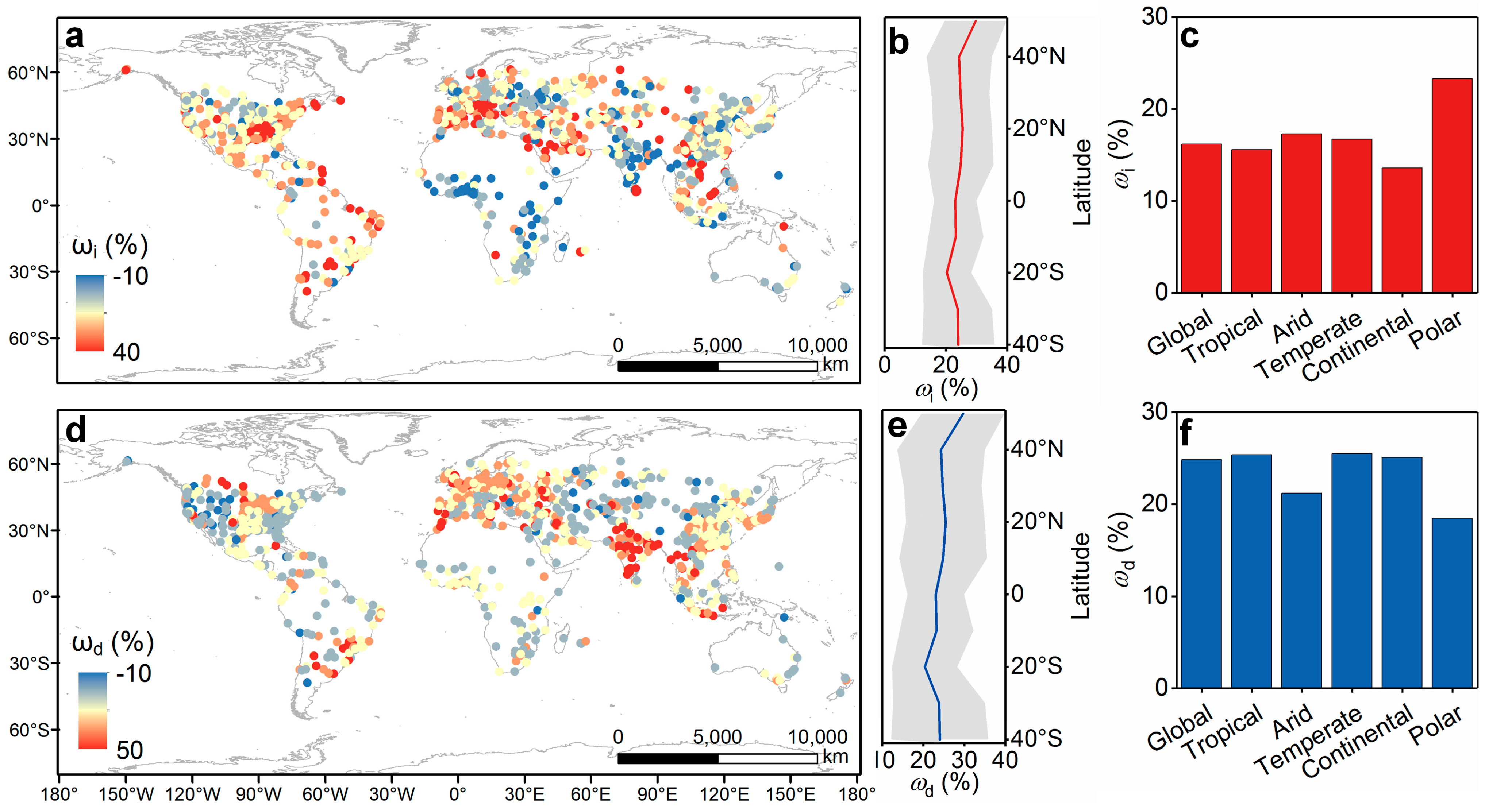
3.2. Dominant Determinants of the Indirect Urbanization Impact on Biodiversity Dynamics

The relationships of ω_i with the mean annual temperature, mean annual precipitation, urbanization intensity, urban green space, and population density across the globe and within climate zones based on a partial correlation analysis are displayed in Figure 5. A significant negative correlation is observed between ω_i and urbanization intensity and population density on a global scale, with the partial correlation coefficients (r) of −0.34 and −0.12 (p < 0.01), respectively. This suggests that biodiversity demonstrates a robust inverse relationship with alterations in urban ecosystems resulting from anthropogenic influences [39]. In contrast, ω_i is positively but statistically insignificantly correlated with climatic factors such as the mean annual temperature and precipitation (Figure 5a). The insensitivity of ω_i to the mean annual temperature and precipitation may be attributed to human intervention, which has the effect of mitigating the limiting impact of these climatic factors on biodiversity in global cities situated in diverse climatic zones.

Our analysis illustrates that the effect magnitudes and directions of these driving variables affecting ω_i exhibit variability across climate zones (Figure 5b–d). In tropical regions, there is a positive correlation between ω_i and urban green space (r = 0.19, p < 0.01), which is consistent with the positive response of biodiversity to the urban green space observed in previous studies [38]. Conversely, ω_i is negatively correlated with urbanization intensity (r = −0.50, p < 0.01) and population density (r = −0.18, p < 0.01). This is likely due to the replacement of natural surfaces with built-up areas resulting from increases in urban expansion and population growth [40,41], which reduces the positive response of biodiversity to urban environments. In the arid region, the partial correlation coefficients r for urbanization intensity and mean annual precipitation are found to be −0.35 and −0.20 (p < 0.01), respectively, indicating a negative effect on ω_i. Conversely, a positive correlation was observed between ω_i and the mean annual temperature (r = 0.15, p < 0.01). In the temperate zone, climatic factors such as the mean annual temperature and precipitation have a negligible effect on ω_i. Conversely, ω_i is predominantly anthropogenic factors, as evidenced by the negative effect of urbanization intensity and population density on ω_i, with r values of −0.32 and −0.10 (p < 0.01), respectively. In the continental zone, there is a significant relationship between the mean annual temperature and precipitation and ω_i (p < 0.05), most likely because of low temperature and water availability on biodiversity dynamics in cold environments [42]. The significant relationship between urbanization intensity and ω_i (r = −0.24, p < 0.01) in cold regions suggests that the indirect effects of urbanization on biodiversity are particularly pronounced in cold cities with a high degree of urban management. These analyses demonstrate that both climatic and anthropogenic factors exert a combined influence on ω_i. In most regions, anthropogenic factors account for a greater proportion of the variation in ω_i than climatic factors.

3.3. The Indirect Impact Between Cities at Different Biodiversity and Development Levels

We compared the indirect impact ω_i in cities with different levels of biodiversity and development (Figure 6). For the purposes of comparison, the cities were classified into three categories according to their BIIs (or GDP): low BII (low GDP), medium BII (medium GDP), and high BII (high GDP). This categorization was based on the ascending order of the mean BII (or mean GDP) of cities within the 0–33rd, 34th–66th, and 67th–100th percentile ranges. The mean ω_i (22.24%) in low-biodiversity cities is greater than that observed in medium- (14.88%) and high-biodiversity cities (11.54%) (Figure 6a). Notably, the mean ω_i in low-biodiversity cities is almost twice that in high-biodiversity cities. This indicates that future endeavors should prioritize low-biodiversity areas where more effective optimization strategies are required to reverse the biodiversity decline caused by urbanization. Furthermore, the mean ω_i (18.18%) in cities with medium levels of development is greater than that observed in cities with low (15.34%) and high (15.04%) levels of development (Figure 6b). This discrepancy may be attributed to the different stages of urban development. In cities with medium levels of development, the phenomenon of rapid urban expansion exerts a more pronounced ω_i than in cities with low levels of development. The relatively lower ω_i in cities with high levels of development compared to those with medium levels of development is likely due to the provisioning and regulating services of biodiversity conservation in these developed areas [17,43]. These findings suggest that urban biodiversity management should focus more on cities with medium levels of development, with a particular focus on cities with a low degree of biodiversity.

4. Discussion

4.1. Direct and Indirect Impacts at the Global Cities

By combining global grid BII data with a conceptual framework to differentiate between the direct and indirect impacts of urbanization on biodiversity (ω_d and ω_i), we conducted a comprehensive investigation into the spatial distribution of ω_d and ω_i across 1523 global cities.

The results show that urbanization has had widespread positive direct and indirect impacts on urban biodiversity around the world. Previous studies have investigated the impact of urbanization on biodiversity in specific locations, with distinct emphases: references [44,45] primarily examined direct impacts (ω_d) through mechanisms like habitat modification and species selection, while reference [1] focused on indirect impacts (ω_i) mediated by socio-ecological interactions and policy frameworks. However, they did not offer an explicit differentiation between ω_d and ω_i using a well-defined quantitative criterion. The present study demonstrates that the global mean ω_d and ω_i are estimated to be 24.85 ± 9.97% and 16.18 ±10.92%, respectively (Figure 4). In general, more than 99% of the world’s cities exhibit a positive ω_d, indicating a decline in biodiversity resulting from the replacement of natural habitats caused by urbanization. Our findings are consistent with those of existing studies at different scales that have indicated a widespread adverse effect of urbanization on biodiversity [1]. Furthermore, over 86% of cities worldwide exhibit a positive ω_i, indicating that urbanization in the vast majority of cities leads to localized climate changes and other environmental alterations due to human activities, which accelerate the degradation of vegetation and, consequently, contribute to the rapid decline of biodiversity. This finding aligns with previous studies that demonstrated a reduction in biodiversity levels in urban areas relative to the surrounding rural areas [29,45]. More importantly, the paucity of scientific studies on ω_i is concerning, as our results indicate that ω_i can be even more substantial for biodiversity than ω_d in more than 33% of the world’s cities (Figure S3).

It is noteworthy that this study found that the indirect impact (ω_i) of most African cities is significantly lower than that of other highly urbanized regions (e.g., the eastern United States and Western Europe). This phenomenon may be driven by multiple factors. Africa has experienced a period of rapid urbanization in recent years [46], but the fragmented distribution and disorganization of built-up areas may limit the indirect pressures on biodiversity from existing urban environments [47]. And the higher proportion of green space in African cities (e.g., informal agricultural land or nature reserves) may provide temporary refuges for organisms, thereby reducing the cumulative effect of indirect impacts [48,49]. Additionally, the background climate in some parts of Africa (e.g., tropical and arid areas) may serve as a buffer against the indirect interference of urbanization on ecological processes by regulating vegetation recovery capacity or species adaptability [50]. For instance, high precipitation and natural vegetation cover in tropical regions may partially offset the impact of habitat fragmentation caused by urban expansion [15,38]. Future research should combine regional-scale social-ecological data to further explore the uniqueness of urban biodiversity responses in special regions and their implications for sustainable planning.

4.2. Differences in Control Factors of Indirect Effects

Our study demonstrates the combined effects of climate and anthropogenic influences on biodiversity through the indirect impacts of urbanization in cities around the world. Numerous studies have examined the patterns and causes of ω_d on global biodiversity [1,51]. In contrast to ω_d, the drivers of ω_i, in terms of climatic and anthropogenic factors, have received relatively little attention. Our findings demonstrate that climatic and anthropogenic factors exert a joint influence on ω_i across global cities (Figure 5). A statistically significant negative correlation was identified between ω_i and urbanization intensity and population density. This result can be explained by the increase in impervious surfaces during urbanization, which leads to habitat fragmentation and loss. This fragmentation has the potential to disrupt ecological processes (e.g., species dispersal and gene flow), thereby exacerbating biodiversity decline. Furthermore, high population density is often accompanied by an increase in anthropogenic activities (e.g., pollution, resource extraction, and habitat modification), which further exacerbates pressure on urban ecosystems. Consequently, the combined effect of population density and urbanization intensity on microclimatic conditions, soil properties, and water availability creates an environment that is suboptimal for native species [13].

However, we observed considerable variations in the drivers of ω_i across climate zones. The differences can be attributed to a combination of factors, including climatic constraints, urbanization patterns, and the inherent ecological resilience of each region. In the polar regions, which exhibit the highest ω_i (23.27%) (Figure S2), the pronounced sensitivity may stem from the vulnerability of the ecosystems adapted to cold environments and their limited capacity to buffer anthropogenic disturbances. Even moderate urbanization in these areas can destabilize permafrost, alter microclimates, and reduce habitat connectivity for specialized species, thereby amplifying biodiversity loss beyond the direct effects of habitat replacement [52]. Furthermore, polar ecosystems typically feature low species redundancy, making them exceptionally sensitive to indirect stressors such as temperature fluctuations and soil degradation induced by urban heat islands or infrastructure development [51,53]. In contrast, continental climate zones display the lowest ω_i (13.60%), likely due to their inherent climatic variability and ecological resilience [54]. The pronounced seasonal temperature fluctuations and historical adaptation to disturbances in these regions may render ecosystems more capable of withstanding the indirect impacts of urbanization. Additionally, the lower intensity of urbanization in many continental climate cities (e.g., in Russia) compared to highly urbanized temperate or tropical regions may limit the accumulation of stress factors [6]. However, in arid regions, the relatively high ω_i (17.25%) may reflect the critical limiting factor of water scarcity. Urbanization exacerbates water stress through increased impervious surfaces and groundwater extraction, indirectly leading to habitat degradation even in areas with minimal direct land conversion [55]. This aligns with our finding of a significant negative correlation between the ω_i and precipitation in arid regions (r = −0.20, p < 0.01)(Figure 5b–d), underscoring the role of hydrological changes [56]. Tropical and temperate regions exhibit moderate ω_i values (15.58% and 16.72%, respectively), but their drivers differ. In tropical cities, the positive correlation between ω_i and urban green spaces (r = 0.19, p < 0.01) suggests that well-managed vegetation can partially mitigate indirect effects, while rapid urban expansion and a high population density exacerbate biodiversity decline [57]. Conversely, temperate cities are primarily driven by anthropogenic factors (e.g., urbanization intensity, r = −0.32), as their mild climates facilitate dense human settlements, leading to habitat fragmentation and microclimatic homogenization [58]. These findings highlight how regional climatic thresholds and human interventions interact to shape indirect effects, emphasizing the need for climate-specific conservation strategies [59].

4.3. Policies and Strategies

Our research shows significant associations between indirect urbanization impacts and biodiversity and development levels. The results confirm variations in the ω_i between cities at different levels of biodiversity (Figure 6). The greater ω_i in cities with low biodiversity than in those with high biodiversity emphasizes the urgent necessity for biodiversity planning in areas with limited and uneven biodiversity. Moreover, our findings illustrate that ω_i varies between cities at different stages of development. The greater indirect urbanization effect observed in cities with medium levels of development relative to those with low or high levels of development may be attributed to the rapid expansion of urban areas and inadequate management of biodiversity within these urban environments. These results indicate that the management of urban biodiversity in developing cities is relatively inadequate, whereas the management of urban biodiversity in developed cities (at a relatively mature urbanization stage) is more balanced between urban expansion and biodiversity management [1,60].

Based on the research findings, this paper proposes the following specific policy recommendations and practical strategies to enhance the practical application value of urban biodiversity management. Firstly, for cities with low biodiversity, priority should be given to implementing ecological restoration and recovery plans. Specific measures include: (1) establishing strict ecological protection red lines to ensure the preservation and restoration of critical habitats during urban development; (2) promoting nature-based solutions (NbS) such as constructing urban wetlands, green corridors, and ecological parks to enhance ecological connectivity; and (3) introducing biodiversity offset mechanisms, requiring development projects to compensate for ecological losses, with funds allocated to ecological restoration projects. Secondly, for cities with moderate development levels, the focus should be on the negative impacts of rapid urban expansion on biodiversity. The following measures are recommended: (1) integrating biodiversity conservation into the overall urban planning to ensure the preservation of ecological spaces during urbanization; (2) strengthening the regulation of urban expansion to avoid the destruction of ecologically sensitive areas by disorderly development; and (3) promoting the construction of green infrastructure such as rain gardens, green roofs, and ecological streets to enhance urban ecological resilience.

4.4. Limitations and Future Work

Our study encountered several levels of uncertainty. Firstly, there were potential limitations due to inherent deficiencies in the data itself. It is essential to illustrate the general patterns of biodiversity response to urbanization intensity across global cities based on the global grid BII and ISP data. Nevertheless, the quantification of spatial variation in urban density, compactness, and sprawl within cities [61] by using the ISP remains a challenging endeavor, given that different urban structures and development patterns can lead to complex variations in the indirect impact on biodiversity. The BII was employed to assess the impact of urbanization on biodiversity on a global scale. While BII, as a proxy indicator based on human disturbance intensity, effectively captures the overall trends in changes to biological community structure, its limitations need to be explicitly addressed: (1) In terms of species richness representation, BII primarily reflects the proportion of biomass loss caused by human activities but fails to differentiate the sensitivity of various species. This may lead to an underestimation of the loss of key species with unique ecological functions (e.g., pollinators, top predators) or endemic species [62]. (2) At the functional diversity level, BII does not fully account for the composition of species’ functional traits and their niche differentiation, potentially limiting its ability to reveal the degradation mechanisms of ecosystem services (e.g., nutrient cycling, pollination efficiency) during urbanization [63]. (3) Regarding an ecosystem integrity assessment, BII focuses on the structural characteristics of biological communities but lacks the systematic representation of landscape connectivity, ecological process integrity (e.g., gene flow, population dispersal), and synergistic changes in abiotic factors (e.g., soil microbial communities, hydrological conditions) [64]. It is also important to note that, despite the verification of the core findings through a comparison of the results of existing studies at different scales [1,17,60], this study is mainly reliant on the indirect representation of remote sensing products due to the scarcity of global ground-based experimental data. This results in a lack of direct comparison and verification with ground-based biodiversity data. Consequently, subsequent studies should integrate multi-species indicators, independent datasets and high-resolution ground observations to further verify the reliability of the model. Therefore, to more accurately assess biodiversity dynamics, there is an urgent need to integrate multi-dimensional indicators based on species and ecosystems (e.g., the City Biodiversity Index, CBI) and combine them with remotely sensed functional diversity parameters and socio-ecological indicators to form a comprehensive evaluation framework [65].

Secondly, uncertainties were introduced during the experimental processing. In this study, to standardize the analytical scale, we resampled other remote sensing data to a 100 m resolution to match the grid scale of the BII. While this method preserves the spatial continuity of the data, the spatial heterogeneity of the original low-resolution data may be smoothed during the interpolation process [66]. Moreover, due to the missing impervious surface percentage (ISP) data for 2019 and 2020, we used the 2018 ISP data as a substitute. Although the changes in the ISP between adjacent years are typically small and similar data substitution methods have been commonly used in other studies, this substitution may still introduce some uncertainty. Therefore, future research should further consider these factors to enhance the accuracy and reliability of the findings.

Thirdly, five driving factors were included to investigate the controls of the climatic and anthropogenic factors on indirect impact. However, it should be noted that other environmental factors, such as tree species composition, energy consumption, and air pollution, may also affect biodiversity dynamics in cities [1]. In addition to the climatic and anthropogenic factors, socioeconomic drivers—such as governance frameworks and conservation policies—may play a pivotal role in modulating the indirect effects of urbanization on biodiversity [67]. For instance, cities with robust environmental regulations, green infrastructure requirements, and habitat restoration programs may mitigate biodiversity loss by counteracting the adverse effects of urban expansion [68]. Conversely, regions with fragmented governance or weak enforcement of conservation policies often experience unchecked urban sprawl, exacerbating habitat fragmentation and biodiversity decline [6]. Therefore, it is crucial to investigate the influence of those potential factors on biodiversity. This will facilitate a more profound comprehension of the impact of urbanization on biodiversity.

Finally, as in numerous previous studies [17,60], the influencing factors were analyzed using statistical methods. It would be beneficial for future studies to provide physical explanations for biodiversity responses to urban environments. By comparing the BII response curves of 1523 cities around the world, we found that the relationship between the BII and ISP in the vast majority of cities deviates from the linear trend, indicating that indirect effects are prevalent. The statistical significance of this deviation supports the reliability of the indirect effect analysis. Nevertheless, the linear assumption (zero-impact line) may not apply in all cases. For example, in areas where natural habitat fragmentation or urbanization intensity is extremely high (such as an ISP close to 1), the decline in the BII may show a threshold effect or an accelerating trend [69]. In addition, different ecosystem types (such as forests and grasslands) may respond differently to habitat loss [70]. Notwithstanding the practical benefits of stepwise regression for variable selection, it is important to note the potential risks of overfitting and the possibility of overlooking important variables due to potential multicollinearity issues. Future research can further explore nonlinear models (e.g., machine learning methods) to more accurately describe the relationship between the BII and ISP and the influencing factors.

Despite these inherent uncertainties, our study proposes a well-defined quantitative criterion to distinguish between the direct and indirect impacts of urbanization on biodiversity, thereby offering a novel perspective on the underlying mechanisms of biodiversity responses to urbanization.

5. Conclusions

Urbanization around the world has altered natural habitats and eco-environments, which can have direct and indirect effects on urban biodiversity. Due to limited ground-based experiments, few studies have investigated the impact of urbanization on biodiversity in specific locations, focusing on either direct or indirect effects. However, an explicit distinction between the direct and indirect impacts based on a well-defined quantitative criterion is still lacking. Using the high spatial resolution global 100 m grid biodiversity intactness index data from 2017 to 2020, we examined the direct and indirect effects of urbanization on biodiversity and its dominant drivers in major cities worldwide based on a conceptual framework.

The results show that the indirect effect of urbanization on biodiversity in the world’s major cities tends to be positive, with a global mean indirect effect of 16.18 ± 10.92%. There is a pattern of relatively larger indirect effects in highly urbanized areas such as the eastern United States, Western Europe, and the Middle East, and relatively smaller indirect effects in less urbanized areas such as most parts of Africa. The indirect effects are mainly controlled by urbanization intensity, population density, and background climate, as evidenced by the large variations in the magnitude and direction of these driving variables affecting indirect effects between different climate zones. The responsiveness of biodiversity to urbanization is impacted by the levels of biodiversity and development in cities. The indirect impact of urbanization on biodiversity is greater in lowly biodiverse cities than in highly biodiverse cities. Furthermore, the indirect effects of urbanization on biodiversity are greater in medium-development-status cities than in low- or high-development-status cities. These findings advance our understanding of urban biodiversity dynamics and their underlying mechanisms, thereby providing valuable insights into the management of urban biodiversity and sustainable urban development.

References

1. McDonald, R.I.; Mansur, A.V.; Ascensão, F.; Colbert, M.l.; Crossman, K.; Elmqvist, T.; Gonzalez, A.; Güneralp, B.; Haase, D.; Hamann, M.; et al. Research gaps in knowledge of the impact of urban growth on biodiversity. Nat. Sustain. 2020, 3, 16–24. [Google Scholar] [CrossRef]
2. Zhai, Y.; Zhai, G.; Yu, Z.; Lu, Z.; Chen, Y.; Liu, J. Coupling coordination between urbanization and ecosystem services value in the Beijing-Tianjin-Hebei urban agglomeration. Sustain. Cities Soc. 2024, 113, 105715. [Google Scholar] [CrossRef]
3. Grimm, N.B.; Faeth, S.H.; Golubiewski, N.E.; Redman, C.L.; Wu, J.; Bai, X.; Briggs, J.M. Global Change and the Ecology of Cities. Science 2008, 319, 756–760. [Google Scholar] [CrossRef]
4. Chapman, C.; Hall, J.W. Designing green infrastructure and sustainable drainage systems in urban development to achieve multiple ecosystem benefits. Sustain. Cities Soc. 2022, 85, 104078. [Google Scholar] [CrossRef]
5. Karmanova, T.N.; Feoktistova, N.Y.; Fetisova, E.E.A.; Mosalov, A.A.; Surov, A.V. Urban Ecology: Retrospective and Research Prospects. Biol. Bull. Rev. 2022, 12, 94–105. [Google Scholar] [CrossRef]
6. Seto, K.C.; Güneralp, B.; Hutyra, L.R. Global forecasts of urban expansion to 2030 and direct impacts on biodiversity and carbon pools. Proc. Natl. Acad. Sci. USA 2012, 109, 16083–16088. [Google Scholar] [CrossRef]
7. Simkin, R.D.; Seto, K.C.; McDonald, R.I.; Jetz, W. Biodiversity impacts and conservation implications of urban land expansion projected to 2050. Proc. Natl. Acad. Sci. USA 2022, 119, e2117297119. [Google Scholar] [CrossRef]
8. Fairbairn, A.J.; Meyer, S.T.; Mühlbauer, M.; Jung, K.; Apfelbeck, B.; Berthon, K.; Frank, A.; Guthmann, L.; Jokisch, J.; Kerler, K.; et al. Urban biodiversity is affected by human-designed features of public squares. Nat. Cities 2024, 1, 706–715. [Google Scholar] [CrossRef]
9. McKinney, M.L. Urbanization, Biodiversity, and Conservation: The impacts of urbanization on native species are poorly studied, but educating a highly urbanized human population about these impacts can greatly improve species conservation in all ecosystems. BioScience 2002, 52, 883–890. [Google Scholar] [CrossRef]
10. van Vliet, J. Direct and indirect loss of natural area from urban expansion. Nat. Sustain. 2019, 2, 755–763. [Google Scholar] [CrossRef]
11. Hautier, Y.; Tilman, D.; Isbell, F.; Seabloom, E.W.; Borer, E.T.; Reich, P.B. Anthropogenic environmental changes affect ecosystem stability via biodiversity. Science 2015, 348, 336–340. [Google Scholar] [CrossRef] [PubMed]
12. Newbold, T.; Hudson, L.N.; Hill, S.L.L.; Contu, S.; Lysenko, I.; Senior, R.A.; Börger, L.; Bennett, D.J.; Choimes, A.; Collen, B.; et al. Global effects of land use on local terrestrial biodiversity. Nature 2015, 520, 45–50. [Google Scholar] [CrossRef] [PubMed]
13. Turner, W.R.; Nakamura, T.; Dinetti, M. Global Urbanization and the Separation of Humans from Nature. BioScience 2004, 54, 585–590. [Google Scholar] [CrossRef]
14. Wang, Y.; Zhu, L.; Yang, X.; Zhang, X.; Wang, X.; Pei, J.; Zhou, L.; Luo, Z.; Fang, Q.; Liang, M.; et al. Evaluating the conservation priority of key biodiversity areas based on ecosystem conditions and anthropogenic threats in rapidly urbanizing areas. Ecol. Indic. 2022, 142, 109245. [Google Scholar] [CrossRef]
15. Gibson, L.; Lee, T.M.; Koh, L.P.; Brook, B.W.; Gardner, T.A.; Barlow, J.; Peres, C.A.; Bradshaw, C.J.A.; Laurance, W.F.; Lovejoy, T.E.; et al. Primary forests are irreplaceable for sustaining tropical biodiversity. Nature 2011, 478, 378–381. [Google Scholar] [CrossRef]
16. Nie, Y.; Zhang, X.; Yang, Y.; Liu, Z.; He, C.; Chen, X.; Lu, T. Assessing the impacts of historical and future land-use/cover change on habitat quality in the urbanizing Lhasa River Basin on the Tibetan Plateau. Ecol. Indic. 2023, 148, 110147. [Google Scholar] [CrossRef]
17. Jung, M.; Rowhani, P.; Scharlemann, J.P.W. Impacts of past abrupt land change on local biodiversity globally. Nat. Commun. 2019, 10, 5474. [Google Scholar] [CrossRef]
18. Feng, R.; Wang, F.; Wang, K.; Wang, H.; Li, L. Urban ecological land and natural-anthropogenic environment interactively drive surface urban heat island: An urban agglomeration-level study in China. Environ. Int. 2021, 157, 106857. [Google Scholar] [CrossRef]
19. Krivoguz, D. Geo-spatial analysis of urbanization and environmental changes with deep neural networks: Insights from a three-decade study in Kerch peninsula. Ecol. Inform. 2024, 80, 102513. [Google Scholar] [CrossRef]
20. Araújo, M.B.; Rahbek, C. How Does Climate Change Affect Biodiversity? Science 2006, 313, 1396–1397. [Google Scholar] [CrossRef]
21. Santamouris, M.; Papanikolaou, N.; Livada, I.; Koronakis, I.; Georgakis, C.; Argiriou, A.; Assimakopoulos, D.N. On the impact of urban climate on the energy consumption of buildings. Sol. Energy 2001, 70, 201–216. [Google Scholar] [CrossRef]
22. Leal Filho, W.; Nagy, G.J.; Setti, A.F.F.; Sharifi, A.; Donkor, F.K.; Batista, K.; Djekic, I. Handling the impacts of climate change on soil biodiversity. Sci. Total Environ. 2023, 869, 161671. [Google Scholar] [CrossRef] [PubMed]
23. Amedie, F.A. Impacts of Climate Change on Plant Growth, Ecosystem Services, Biodiversity, and Potential Adaptation Measures. Master’s Thesis, Program Study of Biological and Enviromental Science, University of Gothenberg, Gothenburg, Sweden, 2013. [Google Scholar]
24. Shoo, L.P.; Storlie, C.; Vanderwal, J.; Little, J.; Williams, S.E. Targeted protection and restoration to conserve tropical biodiversity in a warming world. Glob. Change Biol. 2011, 17, 186–193. [Google Scholar] [CrossRef]
25. Midgley, G.; Hannah, L.; Millar, D.; Rutherford, M.; Powrie, L. Assessing the vulnerability of species richness to anthropogenic climate change in a biodiversity hotspot. Glob. Ecol. Biogeogr. 2002, 11, 445–451. [Google Scholar] [CrossRef]
26. Willis, K.J.; Bhagwat, S.A. Biodiversity and Climate Change. Science 2009, 326, 806–807. [Google Scholar] [CrossRef]
27. Zhao, S.; Liu, S.; Zhou, D. Prevalent vegetation growth enhancement in urban environment. Proc. Natl. Acad. Sci. USA 2016, 113, 6313–6318. [Google Scholar] [CrossRef]
28. Zhang, L.; Yang, L.; Zohner, C.M.; Crowther, T.W.; Li, M.; Shen, F.; Guo, M.; Qin, J.; Yao, L.; Zhou, C. Direct and indirect impacts of urbanization on vegetation growth across the world’s cities. Sci. Adv. 2022, 8, eabo0095. [Google Scholar] [CrossRef]
29. Beninde, J.; Veith, M.; Hochkirch, A. Biodiversity in cities needs space: A meta-analysis of factors determining intra-urban biodiversity variation. Ecol. Lett. 2015, 18, 581–592. [Google Scholar] [CrossRef]
30. Li, X.; Gong, P.; Zhou, Y.; Wang, J.; Bai, Y.; Chen, B.; Hu, T.; Xiao, Y.; Xu, B.; Yang, J. Mapping global urban boundaries from the global artificial impervious area (GAIA) data. Environ. Res. Lett. 2020, 15, 094044. [Google Scholar] [CrossRef]
31. Beck, H.E.; Zimmermann, N.E.; McVicar, T.R.; Vergopolan, N.; Berg, A.; Wood, E.F. Present and future Köppen-Geiger climate classification maps at 1-km resolution. Sci. Data 2018, 5, 180214. [Google Scholar] [CrossRef]
32. Scholes, R.J.; Biggs, R. A biodiversity intactness index. Nature 2005, 434, 45–49. [Google Scholar] [CrossRef] [PubMed]
33. Li, F.; Wu, S.; Liu, H.; Yan, D. Biodiversity loss through cropland displacement for urban expansion in China. Sci. Total Environ. 2024, 907, 167988. [Google Scholar] [CrossRef]
34. Gong, P.; Li, X.; Wang, J.; Bai, Y.; Chen, B.; Hu, T.; Liu, X.; Xu, B.; Yang, J.; Zhang, W.; et al. Annual maps of global artificial impervious area (GAIA) between 1985 and 2018. Remote Sens. Environ. 2020, 236, 111510. [Google Scholar] [CrossRef]
35. Chen, J.; Gao, M.; Cheng, S.; Hou, W.; Song, M.; Liu, X.; Liu, Y. Global 1 km × 1 km gridded revised real gross domestic product and electricity consumption during 1992–2019 based on calibrated nighttime light data. Sci. Data 2022, 9, 202. [Google Scholar] [CrossRef]
36. Song, J.; Gasparrini, A.; Wei, D.; Lu, Y.; Hu, K.; Fischer, T.B.; Nieuwenhuijsen, M. Do greenspaces really reduce heat health impacts? Evidence for different vegetation types and distance-based greenspace exposure. Environ. Int. 2024, 191, 108950. [Google Scholar] [CrossRef] [PubMed]
37. Zhang, X.; Alexander, L.; Hegerl, G.C.; Jones, P.; Tank, A.K.; Peterson, T.C.; Trewin, B.; Zwiers, F.W. Indices for monitoring changes in extremes based on daily temperature and precipitation data. WIREs Clim. Change 2011, 2, 851–870. [Google Scholar] [CrossRef]
38. Pereira, P.; Baró, F. Greening the city: Thriving for biodiversity and sustainability. Sci. Total Environ. 2022, 817, 153032. [Google Scholar] [CrossRef]
39. McDonald, R.I.; Kareiva, P.; Forman, R.T.T. The implications of current and future urbanization for global protected areas and biodiversity conservation. Biol. Conserv. 2008, 141, 1695–1703. [Google Scholar] [CrossRef]
40. Gaffin, S.R.; Rosenzweig, C.; Kong, A.Y.Y. Adapting to climate change through urban green infrastructure. Nat. Clim. Chang. 2012, 2, 704. [Google Scholar] [CrossRef]
41. Morton, D.C.; DeFries, R.S.; Shimabukuro, Y.E.; Anderson, L.O.; Arai, E.; del Bon Espirito-Santo, F.; Freitas, R.; Morisette, J. Cropland expansion changes deforestation dynamics in the southern Brazilian Amazon. Proc. Natl. Acad. Sci. USA 2006, 103, 14637–14641. [Google Scholar] [CrossRef]
42. Mantyka-pringle, C.S.; Martin, T.G.; Rhodes, J.R. Interactions between climate and habitat loss effects on biodiversity: A systematic review and meta-analysis. Glob. Change Biol. 2012, 18, 1239–1252. [Google Scholar] [CrossRef]
43. Pereira, H.M.; Martins, I.S.; Rosa, I.M.D.; Kim, H.; Leadley, P.; Popp, A.; van Vuuren, D.P.; Hurtt, G.; Quoss, L.; Arneth, A.; et al. Global trends and scenarios for terrestrial biodiversity and ecosystem services from 1900 to 2050. Science 2024, 384, 458–465. [Google Scholar] [CrossRef]
44. Aronson, M.F.; Lepczyk, C.A.; Evans, K.L.; Goddard, M.A.; Lerman, S.B.; MacIvor, J.S.; Nilon, C.H.; Vargo, T. Biodiversity in the city: Key challenges for urban green space management. Front. Ecol. Environ. 2017, 15, 189–196. [Google Scholar] [CrossRef]
45. Faeth, S.H.; Bang, C.; Saari, S. Urban biodiversity: Patterns and mechanisms. Ann. N. Y. Acad. Sci. 2011, 1223, 69–81. [Google Scholar] [CrossRef] [PubMed]
46. Yao, R.; Cao, J.; Wang, L.; Zhang, W.; Wu, X. Urbanization effects on vegetation cover in major African cities during 2001–2017. Int. J. Appl. Earth Obs. Geoinf. 2019, 75, 44–53. [Google Scholar] [CrossRef]
47. Ayeni, A.O.; Aborisade, A.G.; Onuminya, T.O.; Soneye, A.S.O.; Ogundipe, O.T. Urban Development in Africa and Impact on Biodiversity. Curr. Landsc. Ecol. Rep. 2023, 8, 73–89. [Google Scholar] [CrossRef]
48. Güneralp, B.; Lwasa, S.; Masundire, H.; Parnell, S.; Seto, K.C. Urbanization in Africa: Challenges and opportunities for conservation. Environ. Res. Lett. 2017, 13, 015002. [Google Scholar] [CrossRef]
49. De Vos, K.; Janssens, C.; Jacobs, L.; Campforts, B.; Boere, E.; Kozicka, M.; Leclère, D.; Havlík, P.; Hemerijckx, L.-M.; Van Rompaey, A.; et al. African food system and biodiversity mainly affected by urbanization via dietary shifts. Nat. Sustain. 2024, 7, 869–878. [Google Scholar] [CrossRef]
50. Thorn, J.P.R.; Biancardi Aleu, R.; Wijesinghe, A.; Mdongwe, M.; Marchant, R.A.; Shackleton, S. Mainstreaming nature-based solutions for climate resilient infrastructure in peri-urban sub-Saharan Africa. Landsc. Urban Plan. 2021, 216, 104235. [Google Scholar] [CrossRef]
51. Post, E.; Alley, R.B.; Christensen, T.R.; Macias-Fauria, M.; Forbes, B.C.; Gooseff, M.N.; Iler, A.; Kerby, J.T.; Laidre, K.L.; Mann, M.E.; et al. The polar regions in a 2 °C warmer world. Sci. Adv. 2019, 5, eaaw9883. [Google Scholar] [CrossRef]
52. Hugelius, G.; Loisel, J.; Chadburn, S.; Jackson, R.B.; Jones, M.; MacDonald, G.; Marushchak, M.; Olefeldt, D.; Packalen, M.; Siewert, M.B.; et al. Large stocks of peatland carbon and nitrogen are vulnerable to permafrost thaw. Proc. Natl. Acad. Sci. USA 2020, 117, 20438–20446. [Google Scholar] [CrossRef] [PubMed]
53. Stewart, I.D.; Oke, T.R. Local Climate Zones for Urban Temperature Studies. Bull. Am. Meteorol. Soc. 2012, 93, 1879–1900. [Google Scholar] [CrossRef]
54. Oliver, T.H.; Heard, M.S.; Isaac, N.J.B.; Roy, D.B.; Procter, D.; Eigenbrod, F.; Freckleton, R.; Hector, A.; Orme, C.D.L.; Petchey, O.L.; et al. Biodiversity and Resilience of Ecosystem Functions. Trends Ecol. Evol. 2015, 30, 673–684. [Google Scholar] [CrossRef] [PubMed]
55. Jones, J.A.; Creed, I.F.; Hatcher, K.L.; Warren, R.J.; Adams, M.B.; Benson, M.H.; Boose, E.; Brown, W.A.; Campbell, J.L.; Covich, A.; et al. Ecosystem Processes and Human Influences Regulate Streamflow Response to Climate Change at Long-Term Ecological Research Sites. BioScience 2012, 62, 390–404. [Google Scholar] [CrossRef]
56. Sala, O.E.; Stuart Chapin, F.; Armesto, J.J.; Berlow, E.; Bloomfield, J.; Dirzo, R.; Huber-Sanwald, E.; Huenneke, L.F.; Jackson, R.B.; Kinzig, A.; et al. Global Biodiversity Scenarios for the Year 2100. Science 2000, 287, 1770–1774. [Google Scholar] [CrossRef]
57. Elmqvist, T.; Setälä, H.; Handel, S.N.; van der Ploeg, S.; Aronson, J.; Blignaut, J.N.; Gómez-Baggethun, E.; Nowak, D.J.; Kronenberg, J.; de Groot, R. Benefits of restoring ecosystem services in urban areas. Curr. Opin. Environ. Sustain. 2015, 14, 101–108. [Google Scholar] [CrossRef]
58. Aronson, M.F.J.; La Sorte, F.A.; Nilon, C.H.; Katti, M.; Goddard, M.A.; Lepczyk, C.A.; Warren, P.S.; Williams, N.S.G.; Cilliers, S.; Clarkson, B.; et al. A global analysis of the impacts of urbanization on bird and plant diversity reveals key anthropogenic drivers. Proc. R. Soc. B Biol. Sci. 2014, 281, 20133330. [Google Scholar] [CrossRef]
59. Díaz, S.; Settele, J.; Brondízio, E.S.; Ngo, H.T.; Agard, J.; Arneth, A.; Balvanera, P.; Brauman, K.A.; Butchart, S.H.M.; Chan, K.M.A.; et al. Pervasive human-driven decline of life on Earth points to the need for transformative change. Science 2019, 366, eaax3100. [Google Scholar] [CrossRef] [PubMed]
60. Ren, Q.; He, C.; Huang, Q.; Shi, P.; Zhang, D.; Güneralp, B. Impacts of urban expansion on natural habitats in global drylands. Nat. Sustain. 2022, 5, 869–878. [Google Scholar] [CrossRef]
61. Batty, M. The Size, Scale, and Shape of Cities. Science 2008, 319, 769–771. [Google Scholar] [CrossRef]
62. Martin, P.A.; Green, R.E.; Balmford, A. The biodiversity intactness index may underestimate losses. Nat. Ecol. Evol. 2019, 3, 862–863. [Google Scholar] [CrossRef]
63. Cardinale, B.J.; Duffy, J.E.; Gonzalez, A.; Hooper, D.U.; Perrings, C.; Venail, P.; Narwani, A.; Mace, G.M.; Tilman, D.; Wardle, D.A.; et al. Biodiversity loss and its impact on humanity. Nature 2012, 486, 59–67. [Google Scholar] [CrossRef] [PubMed]
64. Pettorelli, N.; Laurance, W.F.; O’Brien, T.G.; Wegmann, M.; Nagendra, H.; Turner, W. Satellite remote sensing for applied ecologists: Opportunities and challenges. J. Appl. Ecol. 2014, 51, 839–848. [Google Scholar] [CrossRef]
65. Uchiyama, Y.; Kohsaka, R. Application of the City Biodiversity Index to populated cities in Japan: Influence of the social and ecological characteristics on indicator-based management. Ecol. Indic. 2019, 106, 105420. [Google Scholar] [CrossRef]
66. Smid, M.; Costa, A.C. Climate projections and downscaling techniques: A discussion for impact studies in urban systems. Int. J. Urban Sci. 2018, 22, 277–307. [Google Scholar] [CrossRef]
67. Nilon, C.H.; Aronson, M.F.J.; Cilliers, S.S.; Dobbs, C.; Frazee, L.J.; Goddard, M.A.; O’Neill, K.M.; Roberts, D.; Stander, E.K.; Werner, P.; et al. Planning for the Future of Urban Biodiversity: A Global Review of City-Scale Initiatives. BioScience 2017, 67, 332–342. [Google Scholar] [CrossRef]
68. Dearborn, D.C.; Kark, S. Motivations for Conserving Urban Biodiversity. Conserv. Biol. 2010, 24, 432–440. [Google Scholar] [CrossRef]
69. Zhang, G.; Deng, C.; Liu, Y. Ecological carrying capacity assessment incorporating ecosystem service flows. Environ. Rev. 2024, 32, 592–610. [Google Scholar] [CrossRef]
70. Yan, Y.; Jarvie, S.; Liu, Q.; Zhang, Q. Effects of fragmentation on grassland plant diversity depend on the habitat specialization of species. Biol. Conserv. 2022, 275, 109773. [Google Scholar] [CrossRef]
Figure 1. Selected 1523 cities with an urban area exceeding 100 km2, located in five climate zones, including tropical, arid, warm temperate, continental, and polar.
Remotesensing 17 00956 g001
Figure 2. A conceptual diagram illustrating the direct and indirect impacts of urbanization on biodiversity along the gradient of urbanization intensity (β), which is inspired by the work of Refs. [27,28]. The background color transitions from green to gray in order to represent the spatial gradient from rural to urban areas, characterized by an increase in urbanization intensity (associated with the expansion of urban built areas) and, therefore, a reduction in natural habitats. The global biodiversity intactness index (BII) data and impervious surface percentage (ISP) data are overlaid to characterize the relationship between biodiversity conditions (represented by the BII) and urbanization intensity (represented by the ISP). The blue points represent the observed BII (Bobs) values, while the solid blue line represents the regression fitting line of Bobs (Bfit) using a cubic polynomial model. The dashed blue line denotes the BII change along the spatial gradient from rural to urban areas, assuming that it does not have an indirect impact (Bzi; the theoretical zero-impact line). Bu (solid red line) and Bnu (dashed gray line) is the mean BII of the pixels completely covered by vegetated surfaces (β = 0) and the mean BII of the pixels filled by built-up surfaces (β = 1), respectively. The direct (ωd) and indirect (ωi) impacts can be calculated by comparing Bu and Bobs with Bzi, respectively.
Remotesensing 17 00956 g002
Figure 3. The observed BII and EVI along the urban intensity (β) bin with an interval of 0.05. (a) The global BII, (b) global EVI, and (cf) BII in tropical, arid, temperate, and continental climate zones, respectively. For each panel, the thick line denotes the mean BII (or EVI) dynamics of all cities, whereas the thin line denotes the BII (or EVI) dynamics in a specific city.
Remotesensing 17 00956 g003
Figure 4. Spatial pattern of the urbanization-induced indirect (ωi) and direct impacts (ωd) on biodiversity. (a) Global pattern of ωi, (b) latitudinal variation of ωi, (c) climatic pattern of ωi, (d) global pattern of ωd, (e) latitudinal variation of ωd, and (f) climatic pattern of ωd.
Remotesensing 17 00956 g004
Figure 5. The effects of climatic and anthropogenic factors on the indirect urbanization impact (ωi) on biodiversity dynamics of cities globally and across different climate zones, analyzed using the stepwise regression analysis. (ae) represent the global, tropical, arid, temperate, and continental climate zones, respectively. Climatic and anthropogenic factors include the mean annual temperature (AT), mean annual precipitation (PRP), urbanization intensity (UI), urban greenness (UG), and population density (POP). Significance levels are represented by grey (not significant), orange (p < 0.05) and red (p < 0.01).
Remotesensing 17 00956 g005
Figure 6. The indirect impact (ωi) of urbanization on biodiversity in varying cities with different (a) biodiversity and (b) development levels. Different biodiversity and development levels are represented by the BII and GDP, respectively.
Remotesensing 17 00956 g006
Disclaimer/Publisher’s Note: The statements, opinions and data contained in all publications are solely those of the individual author(s) and contributor(s) and not of MDPI and/or the editor(s). MDPI and/or the editor(s) disclaim responsibility for any injury to people or property resulting from any ideas, methods, instructions or products referred to in the content.