Prediction of Vegetation Indices Series Based on SWAT-ML: A Case Study in the Jinsha River Basin

Abstract

Vegetation dynamics significantly influence watershed ecohydrological processes. Physically based hydrological models often have general plant development descriptions but lack vegetation dynamics data for ecohydrological simulations. Solar-induced chlorophyll fluorescence (SIF) and the Normalized Difference Vegetation Index (NDVI) are widely used in monitoring vegetation dynamics and ecohydrological research. Accurately predicting long-term SIF and NDVI dynamics can support the monitoring of vegetation anomalies and trends. This study proposed a SWAT-ML framework, combining the Soil and Water Assessment Tool (SWAT) and machine learning (ML), in the Jinsha River Basin (JRB). The lag effects that vegetation responds to using hydrometeorological elements were considered while using SWAT-ML. Based on SWAT-ML, SIF and NDVI series from 1982 to 2014 were reconstructed. Finally, the spatial and temporal characteristics of vegetation dynamics in the JRB were analyzed. The results showed the following: (1) the SWAT-ML framework can simulate ecohydrological processes in the JRB with satisfactory results (NS > 0.68, R² > 0.79 for the SWAT; NS > 0.77, MSE < 0.004 for the ML); (2) the vegetation index’s mean value increases (the Z value, the significance indicator in the Mann–Kendall method, is 1.29 for the SIF and 0.11 for the NDVI), whereas the maximum value decreases (Z value = −0.20 for SIF and −0.42 for the NDVI); and (3) the greenness of the vegetation decreases (Z value = −2.93 for the maximum value and −0.97 for the mean value) in the middle reaches. However, the intensity of the vegetation’s physiological activity increases (Z value= 3.24 for the maximum value and 2.68 for the mean value). Moreover, the greenness and physiological activity of the vegetation increase in the lower reaches (Z value = 3.24, 2.68, 2.68, and 1.84 for SIF_max, SIF_ave, NDVI_max, and NDVI_ave, respectively). In the middle and lower reaches, the connection between the SIF and hydrometeorological factors is stronger than that of the NDVI. This research developed a new framework and can provide a reference for complex ecohydrological simulation.

1. Introduction

Vegetation dynamics and the hydrological cycle are two key aspects of the ecohydrological processes in a watershed [1]. Vegetation is an essential component of the Earth’s critical zone and terrestrial ecosystems, linking the atmosphere, hydrosphere, and biosphere [2,3,4], controlling water balance, nutrient cycling, and carbon flux, as well as energy exchange and biogeochemical cycling [5,6,7]. Solar-induced chlorophyll fluorescence (SIF) and the Normalized Difference Vegetation Index (NDVI) are regarded as fundamental descriptors for gauging the coverage and growth conditions of vegetation [8] and can help to analyze the connections between ecosystems and hydrometeorology. Predicting the dynamics of SIF and the NDVI in the long term can provide support for accurately capturing vegetation anomalies and changes in trends [9,10]. Therefore, exploring the prediction of SIF and NDVI contributes to the creation of strategies for ecosystem conservation and water resource management.

A long series of spatiotemporally continuous remote sensing data is also necessary and essential for studying ecohydrological evolution in a larger area [11]. A number of vegetation indicators based on remote sensing such as NDVI, leaf area index (LAI), and enhanced vegetation index (EVI) have been developed and applied widely for vegetation spatial characteristics and dynamics research [12,13,14]. Zheng et al. applied NDVI and LAI for a trend detection and attribution analysis around China [12]. Shi et al. built a regression relationship to examine the NDVI; it was based on machine learning (ML) methods to explore the contributions of climate change and human activities in relation to vegetation changes [14]. Qu et al. utilized EVI for vegetation dynamic detection and attribution in the Yangtze River Basin (YRB) [13]. Remote sensing technology not only provides abundant data sources, but also lays a fundamental foundation for monitoring over large spatial areas [15]. Global NDVI and SIF data products based on remote sensing have emerged. For example, the NDVI data from global inventory modelling and mapping studies (GIMMS) has a spatial resolution of approximately 8 km, a minimum time interval of 15 days, and can be traced back to as early as 1982 [16]. The CSIF data feature a high spatial resolution of 0.05°, starting from 2000, and have a minimum time interval of four days [17]. Xue et al. estimated the ecosystem isohydricity model based on SIF and found that there are distinct seasonal variations in ecosystem isohydricity [18]. Feldman et al. used vegetation indices to explore the sensitivity of large global-scale vegetation to daily rainfall [19]. They discovered that global annual-scale vegetation indices were affected by the frequency and intensity of daily rainfall rather than total annual precipitation. However, the development history of remote sensing technology is relatively short, and its starting time lags behind traditional in situ monitoring methods. This has led to limitations in the accessible time span of remote sensing data, which restricts a comprehensive understanding of the long-term ecohydrological dynamic change process. Meanwhile, affected by factors such as cloud cover and algorithms, uncertainties exist in practical applications, which may lead to understanding bias in the characteristics of specific regions [20,21,22].

In recent years, some studies have employed distributed models or machine learning models to simulate ecohydrological processes [10,23]. The application of distributed models such as the Soil and Water Assessment Tool (SWAT) is based on physical mechanisms, which can comprehensively understand ecohydrological processes [24]. ML is characterized by high accuracy and has been widely applied in various areas, such as the impact of environmental factors on vegetation growth and crop yield prediction [25,26,27]. For example, it can predict crop yields by using satellite and meteorological data, identifying the main influencing factors. However, ML methods lack physical processes, and the simulation accuracy of physical models is not extremely high. The approach that combines physical models with machine learning has been widely used in ecological and hydrological simulations, which integrates the advantages of both physical models and data-driven models [28,29,30]. For example, Wang et al. utilized the SWAT model and machine learning methods to analyze the runoff generation process in a river basin and identify the driving factors [28]. The results showed that precipitation can influence the impact of other factors on runoff generation, and the spatial heterogeneity is evident. The method of coupling distributed physical models with machine learning for ecohydrological prediction can effectively reduce uncertainties due to physical models; this method is based on the mechanism processes and is helpful for understanding ecohydrological processes, while data-driven models can achieve relatively satisfactory results with relatively limited information [31].

The Jinsha River Basin (JRB) is the headwater basin of the Yangtze River in southwest China, located in the eastern and marginal areas of the Qinghai–Tibet Plateau. Due to the huge difference in altitude and topography from upstream to downstream, the climatic conditions in the region vary greatly [32]. This area is characterized by a fragile ecosystem, poor resilience, and sensitivity to climate change [33]. Researchers have indicated that under the influence of climate change, significant changes have occurred in the hydrological and vegetation processes of the JRB [34,35]. The spatial heterogeneity of the impact of driving factors on vegetation dynamics is evident. However, the explanations and spatial heterogeneity of meteorology, hydrology, and the underlying surface in a given area are inadequate during the process of vegetation monitoring and prediction [36]. Therefore, it is necessary to conduct prediction studies on SIF and NDVI in the JRB based on the spatiotemporal heterogeneity of hydrometeorology, so as to better monitor the vegetation dynamics. This not only contributes to the prediction of future evolution trends of vegetation and the analysis of the historical evolution mechanism, but is also of crucial importance for understanding the relationship between the ecosystem and hydrometeorology [8,37,38]. This study provides a scientific basis for ecological environment protection and promotes regional ecological restoration in the JRB.

Therefore, the objective of this research is (1) to propose a framework for vegetation dynamics simulation based on the SWAT-ML method, (2) to reproduce a long series of spatiotemporally continuous SIF and NDVI datasets from 1982 to 2014, and (3) to evaluate the spatial and temporal characteristics of vegetation dynamics in the JRB.

2. Materials and Methods

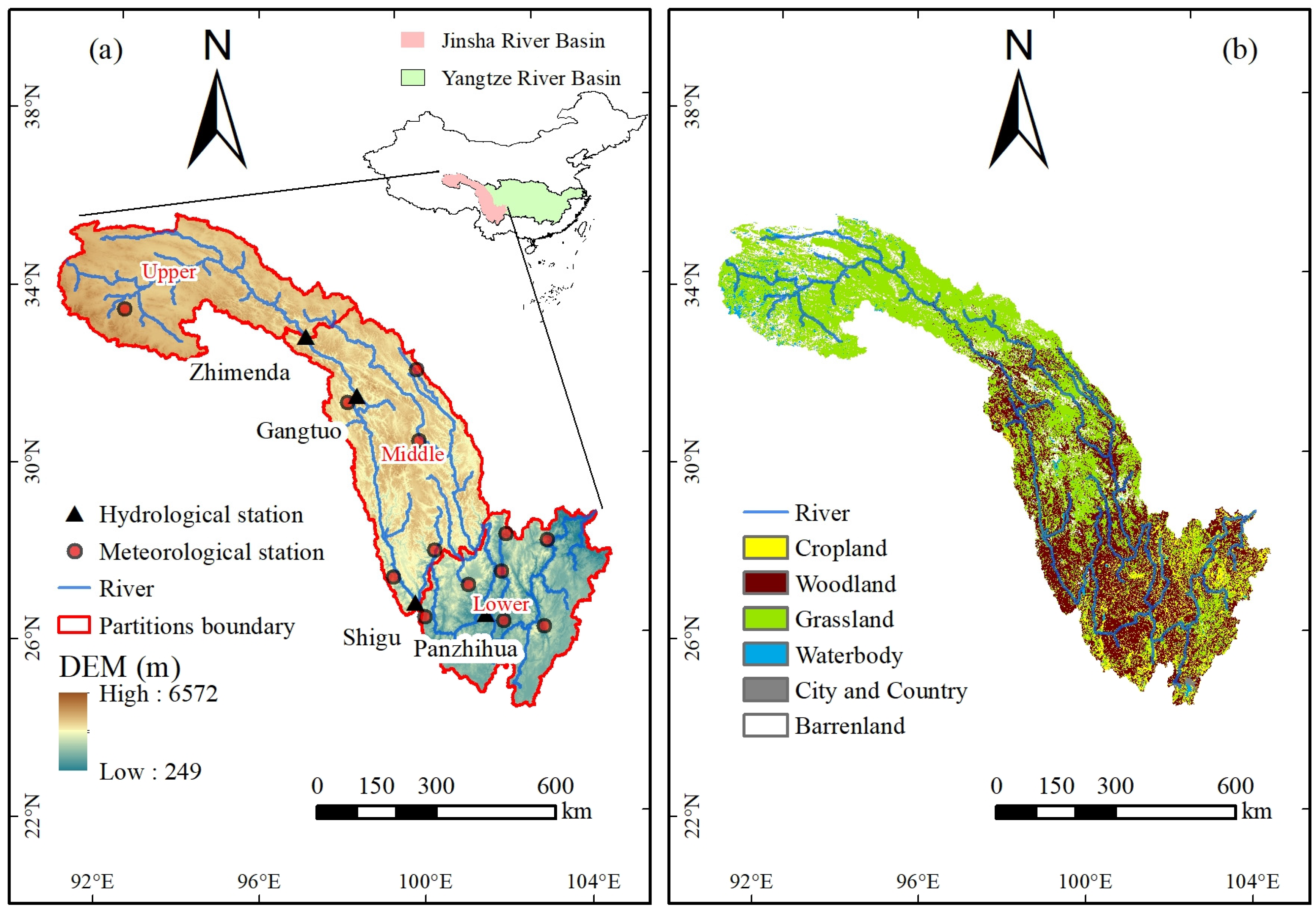
2.1. Study Area and Data

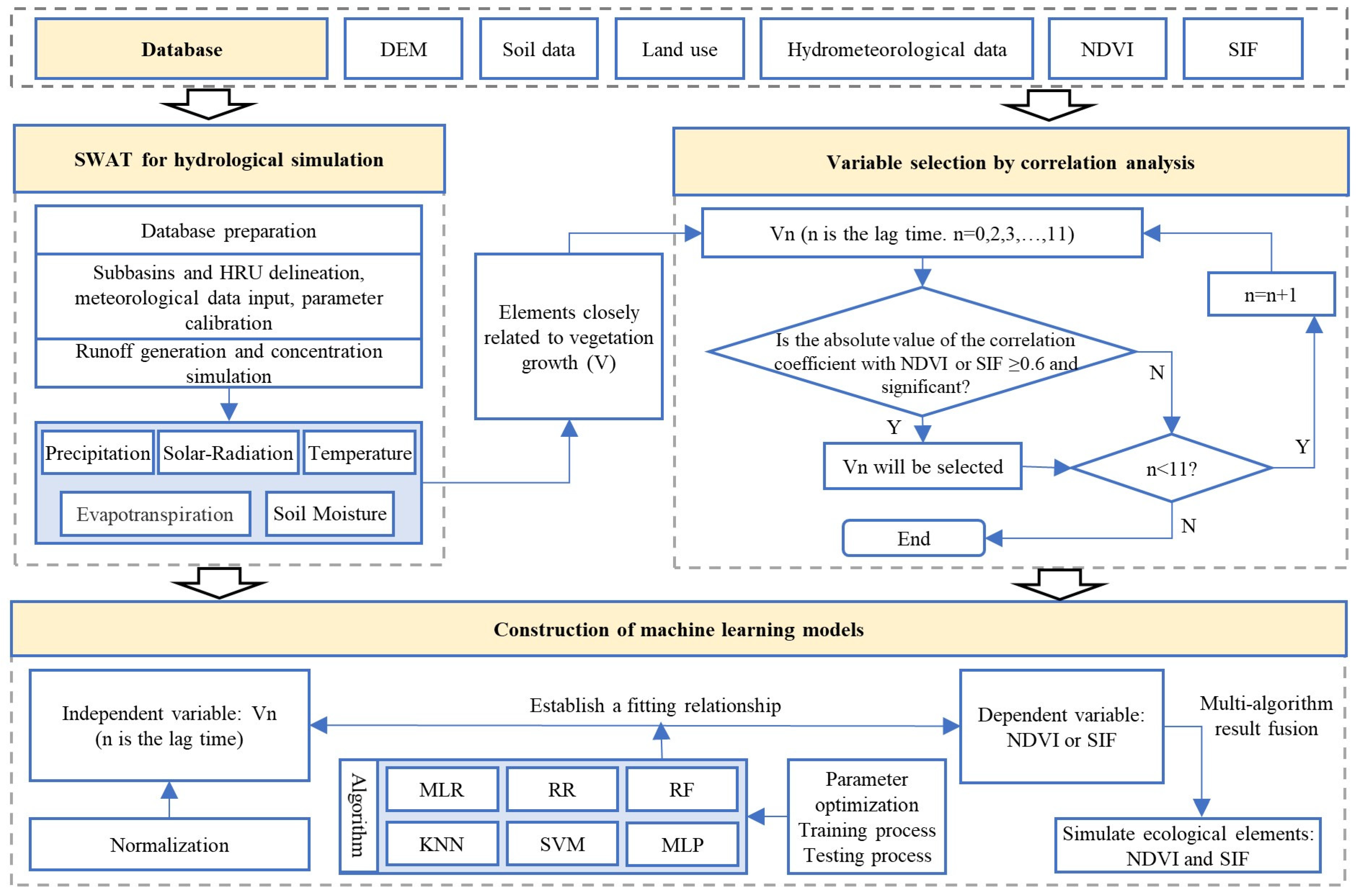
The JRB is the headwater basin of the Yangtze River, which is located in southwestern China, ranging from 90.55°E to 104.94°E longitude and 24.47°N to 35.75°N latitude. The study area covers 47.32 × 10⁴ km², and the altitude varies from 249 to 6572 m, forming an upwards trend from southeast to northwest, as shown in Figure 1a. The spatial distribution of annual precipitation is uneven throughout the basin, which is mainly caused by the subtropical plateau monsoon climate [33]. The upstream area has a low average annual precipitation of approximately 300 mm, while the downstream area has a high average annual precipitation above 1300 mm. Due to the difference in altitude, the annual temperature ranges from a minimum of −5.6 °C upstream to a maximum of 21.9 °C downstream [39]. In this study, the subbasins divided using the SWAT model were taken as the basic units. According to the discrepancies of geographical characteristics such as DEM and vegetation cover, the geometrical interval method was used to divide these subbasins into three regions: upper, middle, and lower. The main vegetation type in the upper reaches of the JRB is grassland (69.46%), the middle reaches contain mainly mixed grassland (52.89%) and forest (36.71%), and the lower reaches are mainly covered by forest (51.42%), grassland (25.47%) and cropland (20.80%). The vegetation in the upper reaches is dominated by alpine vegetation grassland meadows, the middle reaches are dominated by scrub, and the lower reaches are dominated by coniferous forests, mixed coniferous and broad-leaved forests, and cultivated vegetation, as shown in Figure 1b. Comprehensively considering the differences in climatic conditions, vegetation cover, and topographic elevation, the JRB was divided into upstream, midstream, and downstream parts using the Zhimenda and Shigu gauge stations as control stations, as shown in Figure 1a.

The SWAT model requires digital elevation model (DEM) data, land use and land cover (LULC) data, soil data, and hydrological and meteorological data. The DEM data were obtained from the Geospatial Data Cloud (http://www.gscloud.cn/, accessed on 16 June 2022) at a spatial resolution of 90 m. The LULC data were obtained from the Resource and Environmental Science and Data Centre (https://www.resdc.cn/, accessed on 16 June 2022) at a spatial resolution of 1 km. Soil data and soil physical and chemical properties were obtained from the China Soil Database (http://vdb3.soil.csdb.cn, accessed on 10 November 2021). Station monitoring data at the daily scale from 1954 to 2014 were obtained from the National Meteorological Information Centre (http://data.cma.cn, accessed on 5 November 2020) for weather stations, containing precipitation, maximum and minimum temperature, wind speed, solar radiation, and relative humidity data. Monthly runoff station monitoring data were obtained from the Hydrological Yearbook of the People’s Republic of China for the period from 2007 to 2014.

NDVI data from 1982 to 2014 were obtained from Global Inventory Modelling and Mapping Studies (https://daac.ornl.gov/VEGETATION/guides/Global_Veg_Greenness_GIMMS_3G.html, accessed on 20 September 2023) with a spatial resolution of 1/12° and a half-month interval. Solar-induced chlorophyll fluorescence (CSIF) datasets from 2000 to 2014 were provided by Figshare (https://figshare.com/articles/dataset/CSIF/6387494/2, accessed on 8 September 2022) with a spatial resolution of 0.05° and a time interval of 4 days. To eliminate the influence of low-value noise caused by clouds and rain, the maximum value synthesis method [40] was used to obtain the monthly SIF and NDVI sequences.

2.2. Framework

In this work, a framework was developed to simulate the ecohydrological elements of the basin, which is shown in Figure 2. The SWAT model was established to simulate the hydrological process in the JRB and obtain spatial hydrological characteristics such as runoff, evapotranspiration, and soil moisture. ML used the hydrometeorological factors simulated by SWAT as inputs, while SIF and NDVI data were used as the outputs by the regression model, which characterized vegetation growth from 1982 to 2014. Based on this framework, the spatial and temporal distribution and dynamic change characteristics of vegetation based on SIF and NDVI were detected using the Mann–Kendall and Theil–Sen median methods.

2.3. SWAT Model for Hydrological Simulation

SWAT is one of the most widely used semi-distributed basin hydrological models [41]. SWAT hydrological simulations are based on hydrological response units (HRUs) and are suitable for presenting hydrological cycle systems that are limited by spatial and temporal data [42,43]; soil moisture change and evapotranspiration processes, which are closely related to vegetation growth, can be well simulated at the subbasin scale by SWAT. SWAT simulates each hydrological element based on the water balance, as shown in Equation (1).

$$S{M}_t=S{M}_0+\sum _{i=1}^t(P-Q_s-E{T}_a-W_s-Q_g)$$

(1)

where $S{M}_t$ is the soil moisture at moment t. $S{M}_0$ is the initial soil moisture; $P,Q_s,E{T}_a$ are precipitation, surface runoff, and actual evapotranspiration, respectively;$W_s$ is the water entering the vadose zone; $Q_g$ is the return flow.

The SWAT model divides the JRB into 102 subbasins and 247 HRUs based on the digital elevation model (DEM) and underlying surface data. By inputting meteorological data such as precipitation, air temperature, wind speed, and solar radiation, the SWAT model of the JRB was established. This model is used to simulate the hydrological characteristics from 1982 to 2014, including evapotranspiration, soil moisture content, and river runoff for each subbasin. SWAT model parameters were calibrated and validated by the SUFI-2 algorithm in SWAT-CUP [42], using monthly runoff data from 2007 to 2014 from the four gauge stations, i.e., Zhimenda, Gangto, Shigu and Panzhihua, from upstream to downstream, respectively, where the calibration period is from 2007 to 2011 and the validation period is from 2012 to 2014. The deterministic coefficient (R²) [44], Nash–Sutcliffe efficiency coefficient (NS) [45], and relative error (PBIAS) [46] were used to assess the performance of the simulation, as shown in Equations (2)–(4).

$$R^2={\displaystyle \frac{[{\sum }_{i=1}^n(Y_{oi}-{\overline{Y}}_o)(Y_{si}-{\overline{Y}}_s){]}^2}{{\sum }_{i=1}^n(Y_{oi}-{\overline{Y}}_o{)}^2{\sum }_{i=1}^n(Y_{si}-{\overline{Y}}_s{)}^2}}$$

(2)

$$NS=1-{\displaystyle \frac{{\sum }_{i=1}^n(Y_{oi}-Y_{si}{)}^2}{{\sum }_{i=1}^n(Y_{oi}-{\overline{Y}}_o{)}^2}}$$

(3)

$$PBIAS={\displaystyle \frac{{\sum }_{i=1}^n(Y_{s,i}-Y_{o,i})}{{\sum }_{i=1}^n{Y}_{o,i}}}\times 100\%$$

(4)

where $i$ is the rank of the data series; $Y_{oi}$ and $Y_{si}$ are the observed and simulated values of ith, respectively; and ${\overline{Y}}_o$ and ${\overline{Y}}_s$ are the averages of the observations and simulations, respectively.

When R² > 0.7, NS > 0.5, and PBIAS < ±15%, the simulation results and the model performance are considered to be good [47]. A total of 13 sensitive parameters related to the hydrological process in SWAT were selected for model calibration according to sensitivity analysis in SWAT-CUP; the parameter ranges are detailed in

Table 1. Sensitive parameters and ranges for calibration.

Parameters	Definition	Value Range for Calibration	Best Value
CN2	Initial SCS runoff curve number for moisture condition II	[−0.2, 0.2]	−0.19
ALPHA_BF	Baseflow alpha factor (days)	[−0.5, 0.6]	0.56
GW_DELAY	Groundwater delay (days)	[0.8, 1]	242.57
GWQMN	Threshold depth of water in the shallow aquifer required for return flow to occur (mm)	[−0.8, 0.8]	43.01
ALPHA_BNK	Baseflow alpha factor for bank storage	[0, 1]	0.44
ESCO	Soil evaporation compensation factor	[−0.2, 0.4]	0.80
SOL_AWC	Available water capacity of the soil layer	[30, 450]	0.31
SOL_BD	Moist bulk density	[0, 0.2]	−0.15
GW_REVAP	Groundwater "revap" coefficient	[0, 0.3]	0.05
SFTMP	Snowfall temperature	[0, 500]	−0.56
SOL_K	Saturated hydraulic conductivity	[5, 130]	0.39
CH_N2	Manning’s "n" value for the main channel	[−5, 5]	0.18
CH_K2	Effective hydraulic conductivity in main channel alluvium	[0, 1]	44.62

.

2.4. Machine Learning Method for Vegetation Simulation

We selected the main elements of the hydro-thermal conditions that control vegetation growth to predict SIF and NDVI [10,48]. The variables include precipitation (P), evapotranspiration (ET), solar radiation (SR), temperature (T), and soil moisture (SM). The values of these factors for each subbasin were simulated by the SWAT model because of the uneven spatial distribution of meteorological stations. Hydrometeorological elements affect vegetation dynamics with a lagging time, as the growth state of vegetation can be influenced by hydrometeorological factors in the previous few months [49,50]. To improve the signal-to-noise ratio of the input data, reduce the error, improve the accuracy of the results, and reduce the probability of overfitting, before building the machine learning model, the input data are filtered according to the correlation coefficient. The Pearson correlation coefficient (PCC) [51] was calculated as depicted in Equation (5) between SIF or NDVI and Xn (n = 0, 1, 2, …, 11), X is one of the independent variables, and n is defined as the lagging time. This study selected the independent variable with p < 0.05 and the absolute value of the correlation coefficient greater than 0.6 as the input term with n months lagging time and discarded other independent variables.

$$r_{xy}={\displaystyle \frac{\sum _{i=1}^n(X_i-\overline{X})(Y_i-\overline{Y})}{\sqrt{\sum _{i=1}^n{(X_i-\overline{X})}^2}\sqrt{\sum _{i=1}^n{(Y_i-\overline{Y})}^2}}}$$

(5)

Multiple ML algorithms in combination can reduce the uncertainty of the results. According to the commonly used ML algorithms in the previous studies, multiple linear regression (MLR), ridge regression (RR), random forest (RF), K-nearest neighbour (KNN), support vector machine (SVM), and artificial neural network (ANN) models were utilized to predict SIF and NDVI based on hydrometeorological elements between 1982 and 2014. These regression models were created using the scikit-learn package and the Python programming language (v3.6). Specific information for vegetation prediction using machine learning methods is shown in

Table 2. Information for vegetation prediction using machine learning methods.

No.	Dependent Variable	Independent Variable	Machine Learning Algorithms	Regions	Training Period	Testing Period
1	SIF	Tn, SRn, SMn, Pn and ETn (n was the selected lag time by correlation analysis)	MLR, RR, RF, KNN, SVM and MLP	Upper, middle, and lower reaches	2000–2012	2013–2014
2	NDVI				1982–2006	2007–2014

.

The relationship between vegetation growth and meteorological and hydrological elements may vary due to significant differences in vegetation types and hydrothermal conditions in the upper, middle, and lower regions. For that reason, regression models are developed in the upper, middle, and lower reaches, respectively, to ensure the stability and accuracy of the regression model. SIF data from 2000 to 2012 and NDVI data from 1982 to 2006 were used to train models for the upper, middle, and lower reaches, covering 37 upstream subbasins, 30 midstream subbasins, and 35 downstream subbasins, respectively. Models were tested using SIF data from 2013 to 2014 and NDVI data from 2006 to 2014. We further assess the models’ performance on each subbasin of the upper, middle, and lower reaches. Before training the model, to eliminate the dimensional influence and improve the training efficiency, we used Equation (6) to normalize the independent variables; as dependent variables, SIF and NDVI are naturally in the 0–1 interval and do not require normalization.

$${Xnor}_{ij}={\displaystyle \frac{x_{ij}-\min \left(x_j\right)}{\max \left(x_j\right)-\min \left(x_j\right)}}$$

(6)

The selected ML algorithms were presented. In this study, the parameters of ML mainly used the default parameters recommended by the scikit-learn package, and individual parameters were manually adjusted. The multiple linear regression (MLR) method is a statistical technique that can be used to model the relationship between the dependent variable and multiple independent variables [52]. Using the least squares method, a multivariate linear equation is established, which can be achieved by forecasting the dependent variable from the independent variable using Equation (7).

$$\mathrm{Y}=\mathit{B}\mathit{X}+a_0$$

(7)

where B is the coefficient matrix $\left[b_1,b_2,\dots ,b_n\right]$; X is the matrix of independent variables ${[x_1,x_2,\dots ,x_n]}^T$, consisting of the screened hydrometeorological elements; and $a_0$ is a constant offset.

Since there is a certain correlation between hydrometeorological elements, there may be potential covariance between the independent variables. Ridge regression (RR) is a regression method that is used to obtain more realistic and reliable regression coefficients at the cost of losing some information and reducing accuracy by giving up the unbiased nature of the least squares method [53]. The regression relationship for forecasting is the same as MLR, but RR introduces a regularization factor in estimating B, as shown in Equation (8).

$$\widehat{B}=(X_{train}^T{X}_{train}+\alpha I{)}^{-1}{X_{train}}^T{y}_{train}$$

(8)

where $X_{train}$ is the matrix composed of training set independent variables, I is the unit matrix, and $\alpha$ is the regularization factor. A value of 1 was taken in this study.

Random forest (RF) belongs to the bagging class of machine learning algorithms, and the model performance is much better than that of a single weak model due to the integration of many decision trees [54]. In the training phase, random forest uses bootstrap sampling to collect several different sub-training datasets from the input training dataset to train several different decision trees in turn; in the prediction phase, random forest averages the prediction results of multiple internal decision trees to obtain the result. In this study, a random forest consisting of 100 decision trees was used for model training as well as prediction.

K-nearest neighbour (KNN) is a distance-based regression algorithm [55]. The set of k vectors nearest to vector X in the prediction dataset need to be found, weights are then assigned to the k vectors according to their distances, and the value of X as the weighted average of the y values in these k samples can then be predicted. In this study, Euclidean distance is used to calculate the distance between two vectors, as shown in Equation (9), and the k value is set to 5.

$$di{s}_{ij}=\sqrt{\sum _{k=1}^n(x_{ik}-x_{jk}{)}^2}$$

(9)

where $x_{ik}$ and $x_{jk}$ are the kth elements of $X_i$ and $X_j$, respectively.

Support vector machines (SVMs) are used to solve complex nonlinear fitting problems by determining the kernel function number and constructing the optimal hyperplane to solve the complex nonlinear fitting problem [56]. For a dataset, the support vector machine maps the data to a high-dimensional feature space through nonlinear mapping and uses a linear method to find the optimal regression function in the high-dimensional feature space.

Multilayer perceptron (MLP) is a common feedforward artificial neural network with a strong nonlinear mapping capability, adaptive learning capability, and strong robustness [57]. In this study, we built a hidden layer with an input layer and two hidden layers containing 256 neurons. The neurons in the hidden layer use the inner product of the input vector and the weight vector as the independent variables of the activation function; the activation function uses the tanh function; and the weights and biases of each neuron are continuously optimized by the method of error back propagation. The optimizer is chosen as ‘ADAM’, the learning rate is set to 0.001, the loss function is selected as the mean square error (MSE), and the tolerance error is 10⁻⁶.

To evaluate the performance of these models, we chose the Nash–Sutcliffe efficiency coefficient (NS) and mean square error (MSE) as evaluation indicators, as shown in Equations (3) and (10).

$$MSE={\displaystyle \frac{{\sum }_{i=1}^n(y_{Oi}-y_{Si}{)}^2}{n}}$$

(10)

In sequence reconstruction using ML, we selected the average of the output of each model with NS greater than 0.7 as the final value.

2.5. Ecohydrological Trend Analysis

In this work, the Mann–Kendall and Theil–Sen median methods were used to examine the trends in ecohydrological elements, including annual and seasonal precipitation, temperature, SIF, and the NDVI. The annual change trends were analyzed in the upper, middle, and lower reaches of the JRB. The seasonal change trends were calculated in each subbasin to compare the spatial differences in the JRB. The Mann–Kendall method [58,59] is a nonparametric test method that is widely used for the trend testing of hydrometeorological elements. This method has the following advantages: it does not require a specific distribution test for the data series, extremes can be involved in the trend test, and linear trends can be identified. First, a time series set of hydrological elements is constructed as $X=\left\{x_1,x_2,...,x_n\right\}$. Then, the difference function $f\left(x_i-x_j\right) 1\le j<i$ is determined according to Equation (8), and the S value and variance of the S value are calculated using Equations (11)–(13).

$$f(x_i-x_j)=\left\{\begin{array}{c}-1,x_i-x_j<0\\ 0,x_i-x_j=0\\ 1,x_i-x_j>0\end{array}\right.$$

(11)

$$S=\sum _{j=1}^{n-1}\sum _{i=j+1}^{n}f(x_i-x_j)$$

(12)

$$Var\left(S\right)={\displaystyle \frac{1}{18}}n (n-1)(2n+5)$$

(13)

Finally, calculate the Z value as Equation (14). If Z is positive, there is an upwards trend; if Z is negative, there is a downwards trend. If $\left|z\right|>1.96$, the trend is significant at the p < 0.05 confidence level; if $\left|z\right|>2.38$, the trend is significant at the p < 0.01 confidence level.

$$\mathrm{Z}=\left\{\begin{array}{c}{\displaystyle \frac{S-1}{\sqrt{Var\left(S\right)}}},S>0 \\ 0,S=0\\ {\displaystyle \frac{S+1}{\sqrt{Var\left(S\right)}}},S<0\end{array}\right.$$

(14)

The Theil–Sen median method is a robust method of trend calculation with nonparametric statistics [60]. This method is computationally efficient, insensitive to measurement errors and outlier data, and suitable for the trend analysis of long time series data. It can be calculated using Equation (15).

$$slope=Median\left({\displaystyle \frac{x_j-x_i}{j-i}}\right)$$

(15)

where $Median$ represents the median value. If $slope>0$, the series has an upwards trend, and vice versa, a downwards trend.

3. Results

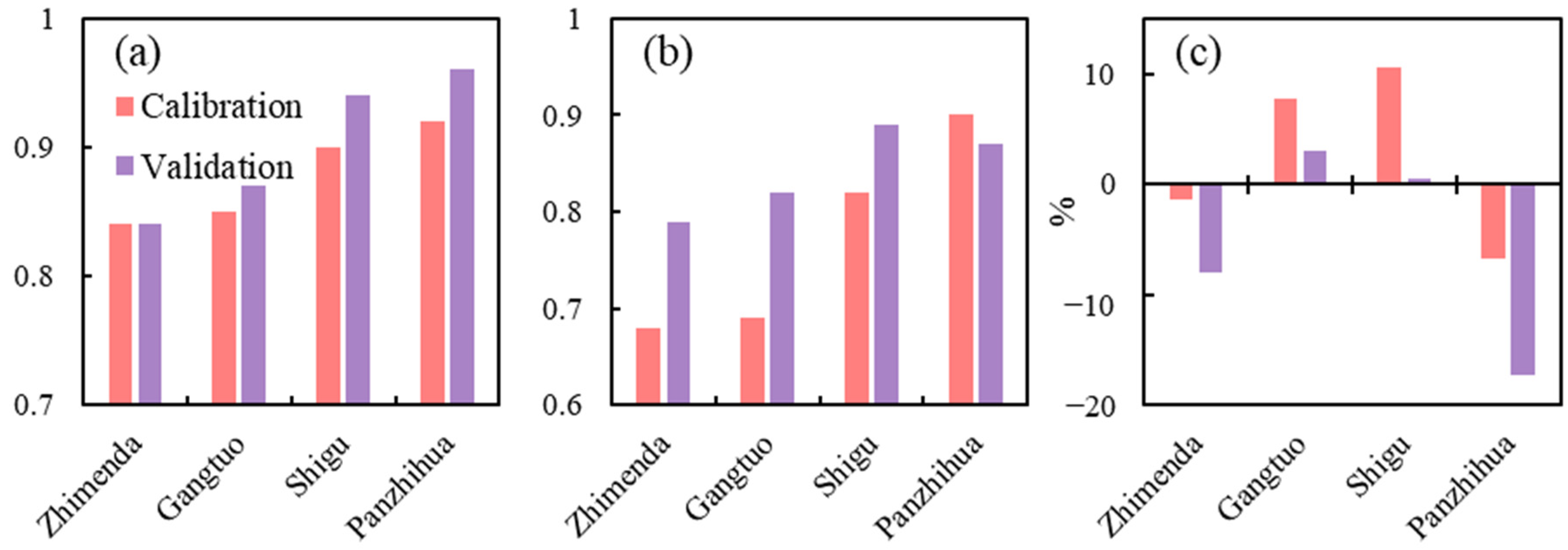
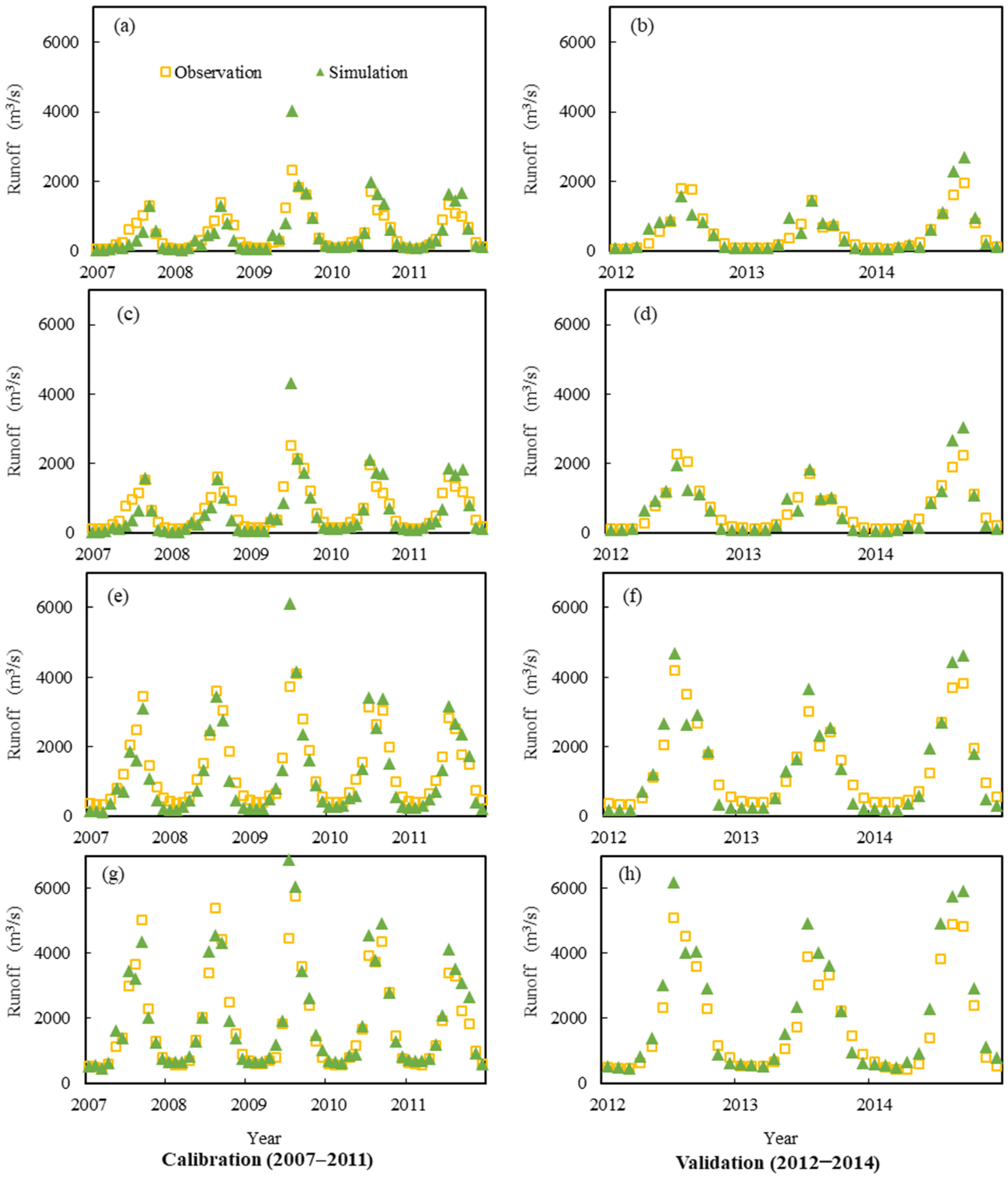
3.1. SWAT Model Calibration and Validation

Figure 3 shows the SWAT model performance at each gauge station in the calibration and validation periods. The results showed that all gauge stations had R² values greater than 0.79, NS values greater than 0.68, and PBIAS absolute values less than 17.35%. The results indicated that the SWAT model can be applied to the hydrological simulation of the JRB [47]. Figure 4 compared the observed and simulated monthly runoff data series. It can be seen that the simulated values generally match the observed values. However, due to the limitations of the accuracy of input data and the model structure, individual numerical simulations may not match the observations. The fitting results of Zhimenda and Gangtuo are generally satisfactory, yet the fitting in some years, such as 2007 and 2008, is less ideal. The fitting for Shigu is rather poor during low-flow periods. For Panzhihua, the overall fitting is good, but it is somewhat off during high-flow periods. This might be attributed to the differences in local underlying surface conditions like topography, soil, vegetation, and meteorological conditions. After the calibration of model parameters related to underlying surface conditions, it is demonstrated that the SWAT model simulation is relatively accurate, has good applicability in the JRB, and can reflect the hydrological cycle process more realistically.

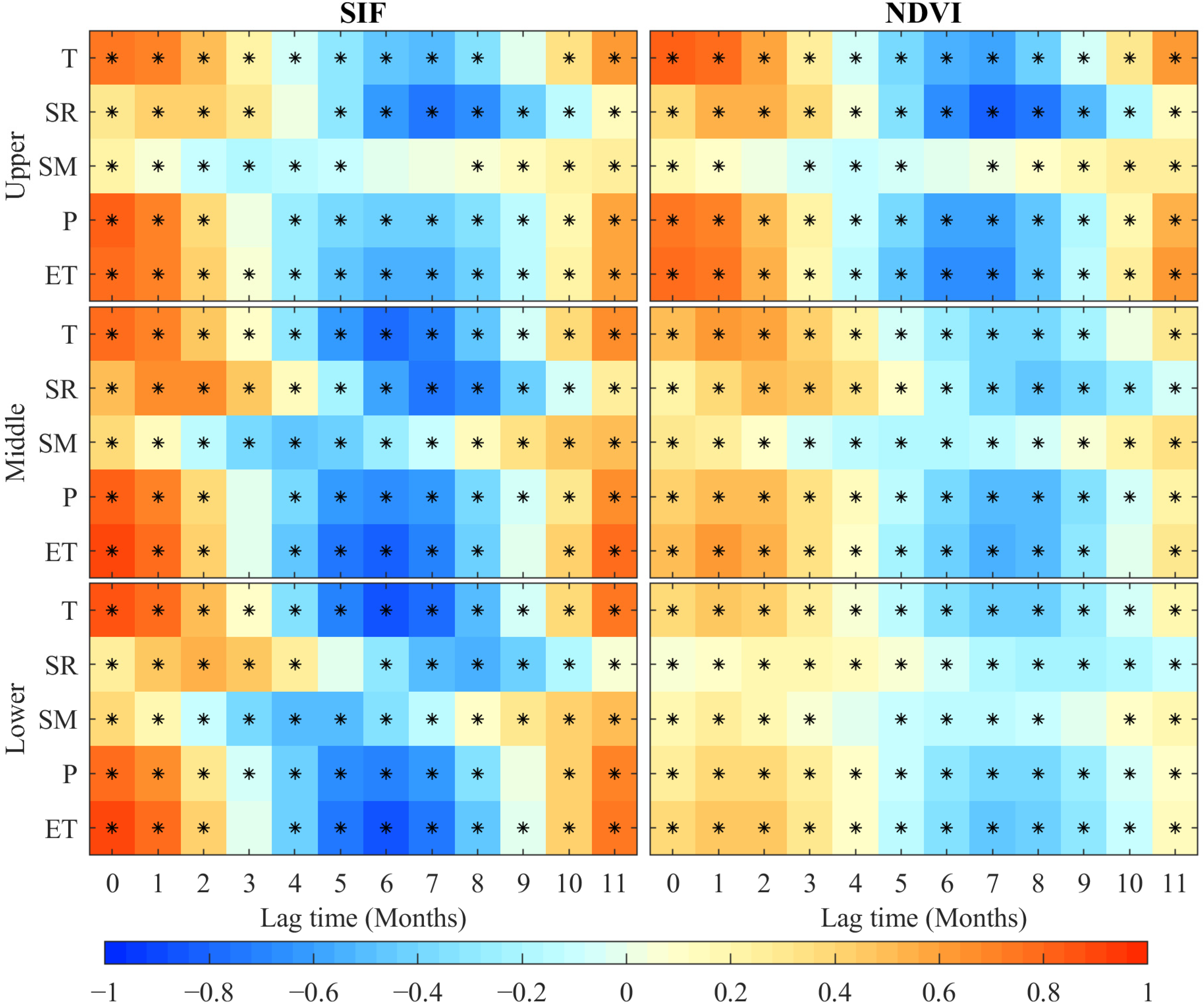
3.2. Correlation Between Vegetation Indicators and Hydrometeorological Elements

Precipitation, temperature, and solar radiation are key meteorological drivers to vegetation change [61,62], and the impact of hydrological factors including evapotranspiration and soil moisture [63,64] on vegetation growth cannot be ignored. Therefore, the hydrometeorological elements including temperature (T), radiation (SR), soil moisture content (SM), precipitation (P), and evapotranspiration (ET) were selected to predict vegetation indices. Previous studies have demonstrated that time-lag effects vary from different vegetation types and climatic factors and the lag-effect timescale ranges from months to seasons and years [49,63,64]. Therefore, for the correlation analysis, a lag time of up to 11 months was taken into consideration to determine the lag time scale. The observed sequences of SIF and NDVI responding to the vegetation condition and the corresponding hydrometeorological elements with lags of 0–11 months are regarded as dependent variables and independent variables, respectively, to analyze the correlation between them. Figure 5 plots the correlation between SIF (a–c), NDVI (d–f), and hydrometeorological elements in the upper, middle, and lower reaches. For the whole basin, T, P, and ET are closely related to SIF. In the upper and middle reaches, the correlation coefficients of the SIF series with the T, P, and ET series with a 0– to 1–month lag are greater than 0.6. Especially in the middle reaches, SIF is more sensitive to SR with a 1- to 2-month lag, and the correlation coefficients reach 0.66 and 0.65, respectively. It is worth noting that the lag effect of SIF on the response of hydrometeorological elements is more obvious, and most of the correlation hypotheses are accepted at the confidence level of p < 0.05. Moreover, in the middle and lower reaches, the correlation coefficients of the SIF series with the T, P, and ET series lagged 5–7 months and 11 months, and are greater than 0.6. The correlation of SIF with meteorological elements in the upstream part is comparable to the correlation of NDVI with meteorological elements. SIF upstream shows a better correlation with P but a worse correlation with T (e.g., $r_{SIF-P_0}=0.81; r_{NDVI-P_0}=0.73;r_{SIF-T_0}=0.74; r_{NDVI-T_0}=0.81$). However, in the midstream and downstream, the correlations between hydrometeorological elements and NDVI are significantly weaker than that with SIF. Although most of the correlation hypotheses are accepted at the confidence level of p < 0.05, the correlation between hydrological elements and NDVI is less than 0.6.

Without considering the lag time, the correlation of NDVI with temperature was better than its correlation with precipitation in the whole basin. In contrast, in the upper and middle reaches, the relationship of SIF with precipitation was closer than that with temperature, indicating that the intensity of vegetation physiological activity was more sensitive to precipitation than to temperature. It has been proven that SIF is more sensitive to climate extremes than NDVI [65], and the correlation between NDVI, SIF, and hydrometeorological elements in our study confirms that under a longer time series scale, SIF was more sensitive to meteorological factors than NDVI in higher vegetation cover regions. NDVI was recognized as demonstrating saturation phenomenon in the areas with lush vegetation and large forest coverage. Saturation phenomenon means that NDVI no longer increases when the leaf area index of vegetation reaches its peak and no longer responds to variations in vegetation dynamics [8,66]. When it comes to SIF, which is an indicator of physiological activity, a closer relationship was observed with the hydrometeorological elements in the middle and lower reaches (Figure 5). It is more reasonable to use SIF when exploring the vegetation response to hydrometeorological elements in regions with a denser vegetation cover.

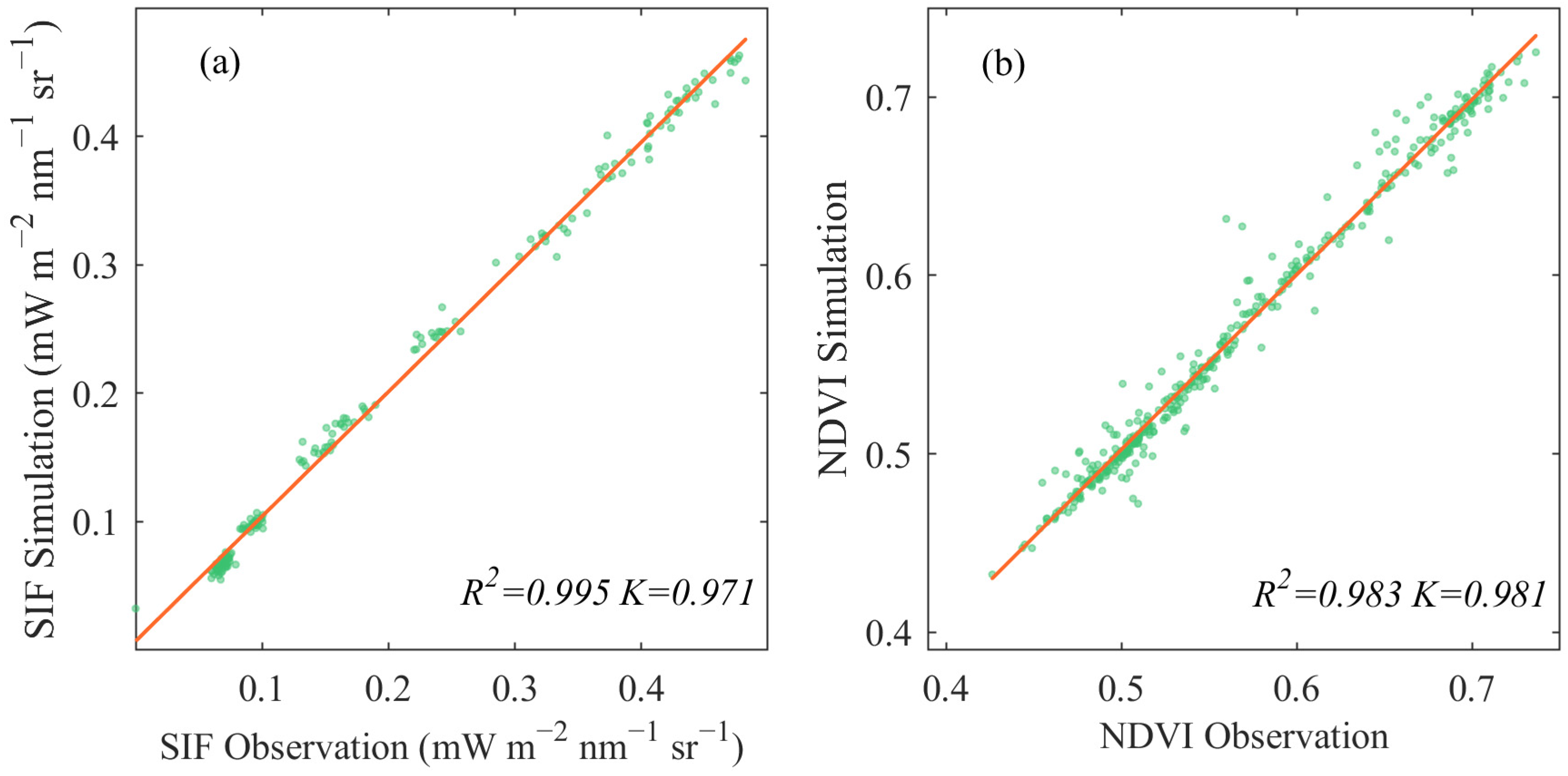
3.3. Vegetation Dynamic Simulation Performance

In this work, ML models were adopted to establish the regression relationship between SIF and the hydrometeorological elements in the upstream, midstream, and downstream regions. A total of 10, 18, and 23 independent variables, which were most relevant independent to SIF (i.e., correlation coefficient > 0.6), were selected as the input for each ML model. For NDVI, since each variable in the middle and lower reaches could not meet the screening requirement (i.e., correlation coefficient greater than 0.6), 13, 9, and 8 independent variables were screened out as the inputs that were most correlated with the dependent variable.

Table 3. Performance of each ML method in the upper, middle, and lower streams.

District	Method	SIF				NDVI
		Train		Test		Train		Test
		NS	MSE	NS	MSE	NS	MSE	NS	MSE
Upper	MLR	0.711	0.005	0.723	0.005	0.721	0.007	0.702	0.007
	RR	0.677	0.005	0.699	0.005	0.709	0.007	0.710	0.007
	RF	0.977	0.000	0.775	0.004	0.978	0.001	0.780	0.005
	KNN	0.896	0.002	0.701	0.005	0.895	0.003	0.687	0.007
	SVM	0.821	0.003	0.817	0.003	0.806	0.005	0.801	0.005
	MLP	0.759	0.004	0.766	0.004	0.791	0.005	0.800	0.005
Middle	MLR	0.880	0.004	0.868	0.005	0.409	0.009	0.320	0.009
	RR	0.850	0.005	0.845	0.005	0.392	0.009	0.316	0.009
	RF	0.985	0.001	0.887	0.004	0.938	0.001	0.426	0.007
	KNN	0.928	0.002	0.897	0.004	0.670	0.005	0.318	0.009
	SVM	0.913	0.003	0.895	0.004	0.518	0.007	0.405	0.008
	MLP	0.892	0.004	0.890	0.004	0.413	0.008	0.312	0.009
Lower	MLR	0.892	0.003	0.860	0.005	0.244	0.007	0.227	0.007
	RR	0.884	0.003	0.855	0.005	0.235	0.007	0.240	0.007
	RF	0.989	0.000	0.862	0.005	0.923	0.001	0.303	0.006
	KNN	0.946	0.002	0.865	0.005	0.590	0.004	0.182	0.007
	SVM	0.928	0.002	0.882	0.004	0.375	0.006	0.328	0.006
	MLP	0.886	0.003	0.831	0.006	0.178	0.007	0.126	0.008

shows the performance of each machine learning model in estimating SIF and NDVI in the upper, middle, and lower reaches. Nearly all machine learning methods achieved good results in the whole basin in retrieving SIF. Except for the ridge regression relationship established upstream, the NS and MSE of each method were >0.7 and <0.005. Among the ML methods, the RF method performs well in the whole basin with a higher NS and a minimum MSE. The main reason for this is that RF is an ensemble learning algorithm; it makes predictions by constructing multiple decision trees and synthesizing their results. This ensemble approach can effectively reduce the variance of the model and mitigate the risk of overfitting, thereby enhancing the model’s stability and generalization ability [54]. For NDVI, both NS and MSE can meet the requirements in the upstream. Also, only MSE meets the accuracy requirements in the midstream and downstream, indicating that the ML-based simulation of NDVI may not be as reliable as that of SIF. This is mainly because the differences in environmental factors between the downstream and upstream regions lead to the fact that apart from being affected by meteorological factors, NDVI is also influenced by human activities. The area of cropland in the downstream reaches is significantly greater than that in the upstream reaches (Figure 1b). Under the influence of human activities, the vegetation conditions represented by NDVI are prone to being affected by environmental factors. In contrast, SIF can reflect the changes in the photosynthetic efficiency of plants, thus, providing information about vegetation dynamics, and is less affected by environmental factors [67,68,69].

In this study, the NS and MSE values of the simulation results of each algorithm in each subbasin were also calculated. The results are shown in Figure 6. The NS values of the simulation results of SIF all approach 1, while the NS values of the simulation results of NDVI are relatively poor. However, the MSE values of both the SIF and NDVI simulation results are close to 0, indicating good performance. The results simulated by multiple machine learning algorithms were integrated, and, ultimately, the SIF and NDVI indices of the JRB were obtained. Figure 7 illustrates the fitting results between the overall simulated values and the measured values in the basin. The measured values and the simulated values are basically distributed around the fitting line, indicating a relatively good simulation result.

3.4. Spatial and Temporal Evolution of Vegetation

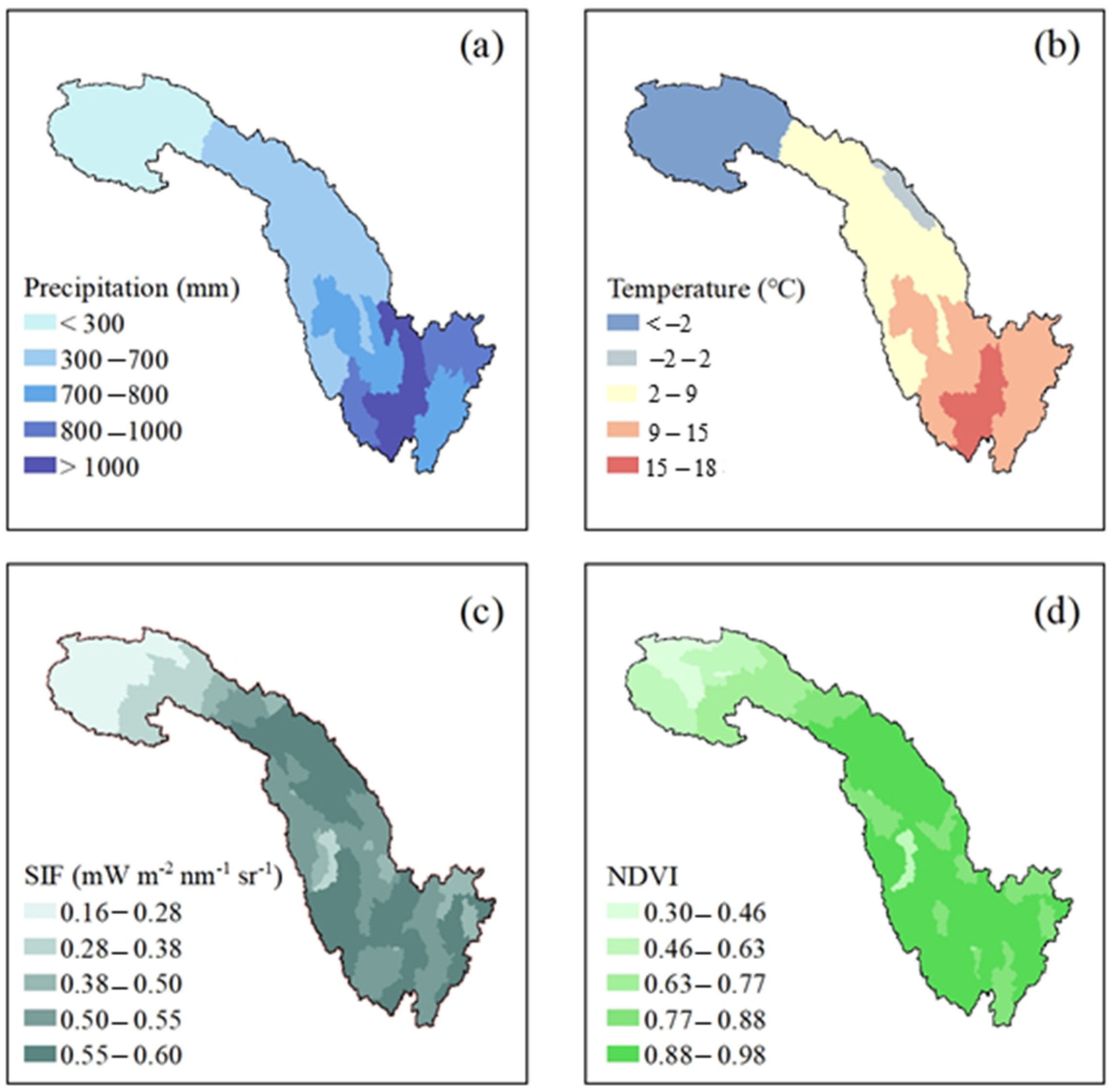
3.4.1. Multiyear Average Vegetation and Meteorological Conditions

Monthly meteorological factors (e.g., precipitation and temperature) and NDVI and SIF series from 1982 to 2014 were compared to reveal the spatial and temporal evolution of vegetation dynamics (Figure 8). The annual values of SIF and NDVI were calculated using the maximum values of the monthly series. Due to the elevation and latitude ranging significantly from upstream to downstream, the hydrothermal conditions in the whole basin demonstrated spatial heterogeneity, which can lead to differences in vegetation distribution. The annual precipitation shows an increasing trend from the upper to the lower reaches. The overall multiyear annual precipitation was 339.0 mm, 684.3 mm, and 938.3 mm for the upper, middle, and lower reaches, respectively. On the contrary, the annual precipitation shows a decreasing trend from the upper to the lower reaches. The multiyear mean temperatures were −1.45 °C, 9.31 °C, and 14.65 °C, respectively. Both the photosynthetic intensity of vegetation characterized by SIF and the “greenness” of vegetation characterized by NDVI showed a decreasing trend from upstream to downstream. The overall multiyear annual SIF values were 0.29, 0.53, and 0.55 for the upper, middle, and lower reaches and the multiyear annual NDVI values were 0.52, 0.83, and 0.85, respectively.

3.4.2. Regional Interannual Vegetation and Climate Change

The trends in climate factors in the upper, middle, and lower regions are shown in

Table 4. The annual climate factor variation in different districts.

District	Climate Factors	Z Value	Slope	Trend
Upper	Precipitation	2.83	4.08	Strongly significant upwards
	Temperature	4.94	0.06	Strongly significant upwards
Middle	Precipitation	−0.45	−0.69	Insignificant downwards
	Temperature	5.09	0.05	Strongly Significant upwards
Lower	Precipitation	−1.50	−2.91	Insignificant downwards
	Temperature	5.50	0.06	Strongly significant upwards

. In general, the whole basin demonstrated a warming trend, with an upwards trend in annual average temperature. Similar conclusions are drawn by Dong et al. [70] and Wang and Zhang [71]. Areas with higher elevation and less precipitation show a significant increasing trend in precipitation, which is consistent with the results obtained by innovative trend analysis [70].

To explore the vegetation dynamic change, the mean and maximum values of SIF and NDVI were calculated in the upper, middle, and lower reaches. The results are shown in

Table 5. The annual vegetation dynamic variation in different districts.

District	Climate Factors	Z Value	Slope	Trend
Upper	SIFmax	−0.20	−1.91 × 10−4	Insignificant downwards
	SIFave	1.29	2.17 × 10−4	Insignificant upwards
	NDVImax	−0.42	−1.81 × 10−4	Insignificant downwards
	NDVIave	0.11	2.32 × 10−5	Insignificant upwards
Middle	SIFmax	3.70	1.25 × 10−3	Strongly significantly upwards
	SIFave	2.46	3.12 × 10−4	Strongly significantly upwards
	NDVImax	−2.93	−7.40 × 10−4	Strongly significantly downwards
	NDVIave	−0.67	−1.75 × 10−4	Insignificant downwards
Lower	SIFmax	3.24	9.21 × 10−4	Strongly significantly upwards
	SIFave	2.68	3.97 × 10−4	Strongly significantly upwards
	NDVImax	2.68	1.04 × 10−3	Strongly significantly upwards
	NDVIave	1.84	4.67 × 10−4	Insignificant upwards

. The wetter and warming trend benefits the average SIF and NDVI. However, a negative influence on the maximum SIF and NDVI was also detected in this region, especially in the upper reaches. Previous studies have indicated that vegetation dynamics would fluctuate within certain thresholds in response to climatic condition changes [72]. The main vegetation type in the upper reaches is highland meadows, for which the growing season is summer, which is often accompanied by heat and humidity. The thermal stress might suppress the physiological activities when the temperature exceeds certain thresholds [73], resulting in a tendency of decreasing SIF.

For the lower reach, both SIF and NDVI showed preferable coordination for both maximum and mean values, although the precipitation showed an insignificant decreasing trend. This means that both the greenness and physiological activity intensity of the vegetation experienced an increasing trend. The increase in temperature may accelerate the decomposition of soil organic matter, which would accelerate the mineralization of nutrients in the soil more easily, promoting the growth of vegetation and offsetting the negative impact of precipitation reduction [74].

For the middle reach, SIF_max and SIF_ave show increasing trends, while NDVI_max and NDVI_ave show decreasing trends. The results indicate that although the greenness of vegetation in the midstream area decreased, the intensity of physiological activity increased. The declining trend in NDVI in the middle reach of the JRB was also detected in other works using NDVI in 1982–2015 [75] and EVI during 2001–2015 [13]. One study aimed to compare different vegetation indexes [37], showing that in the middle reaches of the JRB, most of the PCC values varied from −0.5 to 0 in the growing season. The negative value of PCC means SIF and NDVI show a negative correlation, which may lead to the opposite result from the long-term trend analysis using SIF and NDVI.

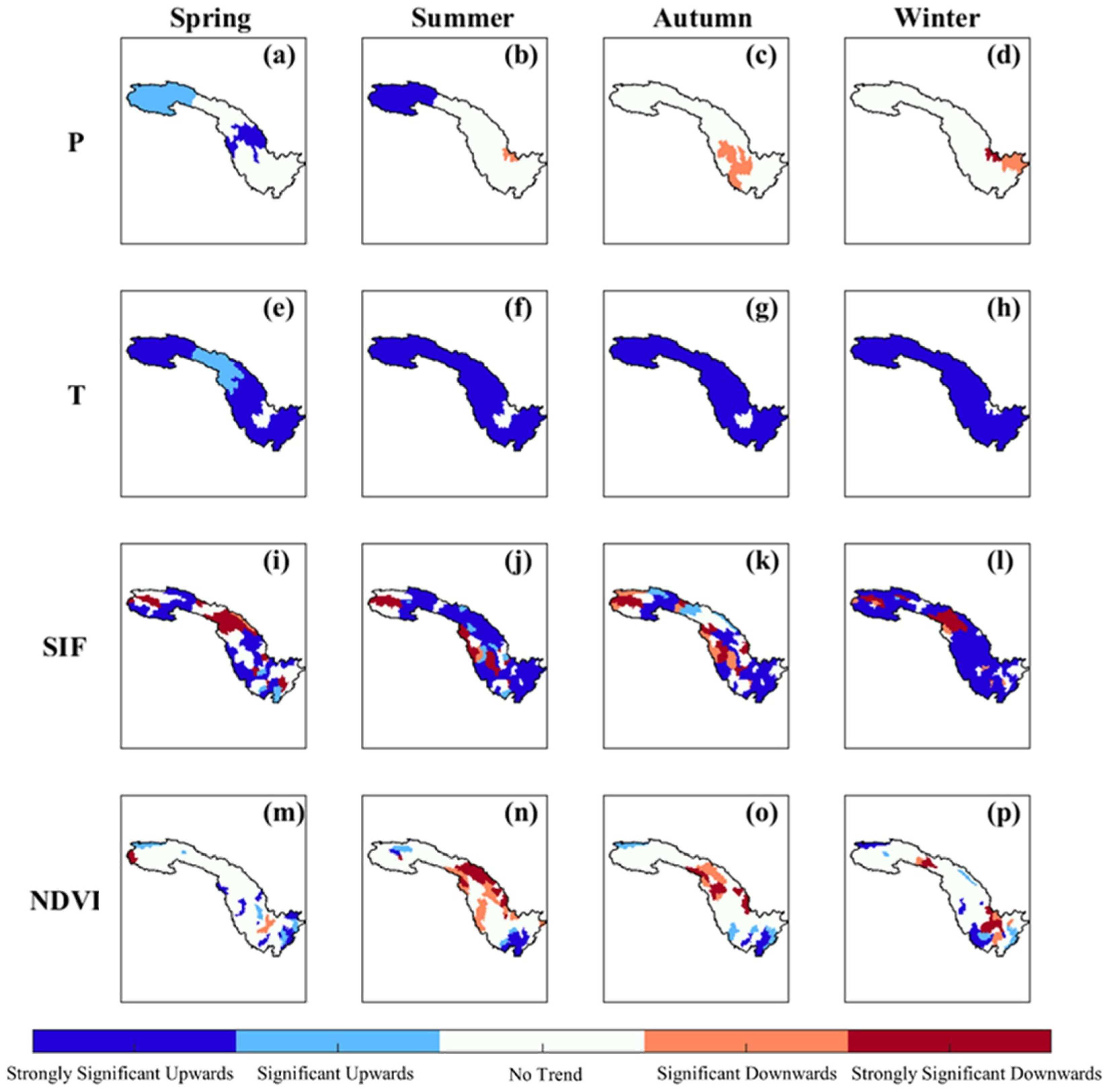
3.4.3. Seasonal Vegetation and Climate Change in Spatial Distribution

To further discuss the seasonal characteristics of each ecohydrological element in each subbasin, the seasonal SIF and NDVI were calculated. The seasonal precipitation and average temperature were also calculated in each subbasin. The slope and significance in each subbasin were analyzed separately and classified into five classes according to the Z value and slope, e.g., strongly significantly upwards ($\left|z\right|>2.38; slope>0$), significant upwards ($\left|z\right|>1.96; slope>0$), significantly downwards ($\left|z\right|>1.96; slope<0$), strongly significantly downwards ($\left|z\right|>2.38; slope<0$), and no significant trend ($\left|z\right|<1.96$).

Figure 9 shows the trend in vegetation dynamics and climatic characteristics in each subbasin. Generally, the evolution of ecohydrological elements at the subbasin scale were consistent with the overall situation, while spatial heterogeneity and seasonal variability was also observed. Credible precipitation increase trends were detected only in the upper and middle reaches in spring, while temperature increased significantly through all seasons over the whole basin. As for the vegetation dynamics, a more significant change was detected for SIF compared to NDVI, which might indicate that the response of physiological activity intensity to changes in hydrometeorological conditions was more sensitive than that of greenness. Temperature and precipitation, as key factors influencing vegetation growth, have nonlinear impacts on vegetation dynamics. Vegetation physiological activities are sensitive to temperature. Under suitable temperature and adequate moisture conditions, vegetation grows vigorously and the values of NDVI and SIF are relatively high. A shortage of precipitation may lead to a decline in vegetation physiological activities, and correspondingly, the values of NDVI and SIF may show a significant decrease [8,65]. Similar research also found that SIF was more sensitive to variation in hydrothermal conditions than NDVI [76]. In the upper reach, 24.32%, 27.03%, and 37.84% of subbasins showed significant or highly significant decreasing trends in SIF in spring, summer, and autumn, respectively, but 64.16% of subbasins showed significant highly increasing trends in winter. SIF values in summer and autumn increased, but decreased in spring and winter, in a large portion of the middle reach. The physiological activity intensity in periods with high values of SIF strengthened, while in periods with low SIF values, it become inactive. In the lower reach, 28.57%, 57.14%, 45.71%, and 54.29% of subbasins showed significant or highly significant increasing trends in SIF in four seasons, respectively. In the middle reach, the overall watershed trend analysis found that greenness decreased but vegetation physiological activity intensity increased in 33.33% of subbasins in summer. The subbasins in which the trends in the indices (SIF and NDVI) showed opposite results were found in the areas with high multiyear NDVI values (high greenness of vegetation), and the inconsistency was more obvious in summer. These results are similar to the conclusion of Zhou et al. [37], who attributed the inconsistency to the saturation of NDVI in regions with high vegetation coverage. NDVI relies on the vegetation projected area within a unit area [8]. As a result, in forests with a high degree of vegetation cover, NDVI has the potential to give an underestimated value of the actual vegetation cover [77]. Considering that the vegetation indices applied in this research, e.g., SIF and NDVI, reflect different vegetation information, their responses to changes in hydrothermal conditions deserve further exploration.

4. Discussion

4.1. Performance of the SWAT-ML in the JRB

In this study, a modelling framework, SWAT-ML, was proposed based on a hybrid hydrological and machine learning method to retrieve ecological and hydrological processes. The SWAT-ML effectively predicted reliable SIF and NDVI series in the JRB. On this basis, the evolutionary characteristics and trends in ecohydrological elements at different scales in the JRB were analyzed. Compared to standalone SWAT applications or purely data-driven ML approaches, SWAT-ML demonstrated superior performance in capturing vegetation dynamics. Validation results showed that the values of R², NS, and MSE indicated that SWAT-ML performed well in the JRB (Figure 3 and Table 3). This hybrid approach leverages physical representation of watershed processes (e.g., runoff partitioning, evapotranspiration) while utilizing data-driven strength in modelling nonlinear vegetation responses to climatic drivers, thereby addressing spatial data limitations common in regions like the JRB.

4.2. Applicability and Potential of the SWAT-ML

The SWAT-ML method provides a new framework for the simulation and prediction of ecohydrological processes. It is of great significance for the historical review analysis and future prediction of ecohydrological components and solves the problem of data limitations preventing ecological monitoring and research. The SWAT-ML method can be applied to regions similar to the JRB. These regions share two main common characteristics. First, the density of in situ monitoring stations for meteorology, hydrology, and ecology is insufficient, and their spatial distribution is uneven. Second, the advantages of data products, such as remote sensing technology, cannot be fully exploited. In the future, we will select typical basins under multiple conditions, including different climates, vegetation, and soil types, on a global scale. We will analyze the applicability of SWAT-ML in multiple typical basins. SWAT-ML has broad application prospects. Research related to watershed ecohydrological processes requires model simulation for support, and the coupling of machine learning and distributed models has obvious complementary advantages. ML is good at handling complex nonlinear relationships, while the distributed model makes full use of the physical characteristics of the watershed. The combination of the two is characterized by adaptability and flexibility, which enhances the ability to simulate complex ecohydrological processes.

4.3. Limitations and Prospects

Some limitations still exist in this study. When using SWAT-ML to predict SIF and NDVI, the impacts of meteorological factors on vegetation were considered, but the interactions between vegetation dynamics and climate were not fully accounted for. The vegetation simulation framework established in this study did not take human activity factors into consideration for the relatively low level of human disturbance of vegetation conditions in the study area. The land use and land cover change is minor compared with climate change [24]. However, in some other regions with strong human intervention, actions such as the grain-for-green programme [78] and ecological construction projects [79] might have an impact on vegetation dynamics. Land use changes alter vegetation cover, affecting evapotranspiration and surface runoff in hydrological processes [1,4]. Agricultural activities artificially change the state of farmland vegetation, modify soil properties, and disrupt the energy balance of the ecosystem [35,36]. The impact of human activities on vegetation and the interaction between environmental factors, including temperature and precipitation and vegetation should be further explored in subsequent studies.

Evaluation indices, such as NS, indicated that SWAT-ML performed well. However, since the output of SWAT serves as the input for ML, there may be error propagation, which represents the next direction for model improvement. Error propagation may lead to the amplification and accumulation of initial errors, resulting in increased model uncertainty and more intricate error patterns. These compounding effects could restrict the applicability of the model across diverse regions and under varying environmental conditions [23,42]. Future studies could mitigate systematic model errors through the following approaches: utilizing high-accuracy datasets with rigorous pre-processing procedures (e.g., outlier detection via isolation forests or wavelet transforms) to eliminate anomalous values; refining the physical model structure through domain-specific sensitivity analysis and parameter optimization algorithms (e.g., Bayesian calibration); and selecting machine learning algorithms with demonstrated robustness in handling nonlinear ecohydrological interactions (e.g., gradient boosting machines or attention-based neural networks) to enhance predictive performance across diverse hydrological regimes.

In our study, one-way coupling was used to extend the SIF-based or NDVI-based vegetation simulation module to the SWAT model. Compared with the LAI-based vegetation module for SWAT, the expanded module captures vegetation dynamics better. It is worth further exploring the use of the two-way coupling approach to optimize the vegetation dynamics module of SWAT to more accurately simulate other ecohydrological processes and to decrease the error propagation.

5. Conclusions

Vegetation dynamics are essential for the ecohydrological process in watersheds and are vital to the ecological security in watersheds. This study developed a framework SWAT-ML hybrid ecohydrological model using SWAT and machine learning in the JRB. We applied SWAT-ML to retrieve the month-by-month SIF and NDVI series from 1982 to 2014. The Mann–Kendall and Theil–Sen methods were used for the trend analysis of vegetation indicators, e.g., SIF and NDVI, and meteorological factors, e.g., precipitation and temperature, in the whole basin. The main conclusions are as follows:

(1)

The SWAT-ML framework can simulate the hydrological process, performing well at each hydrological station satisfactorily (R² > 0.84, NS > 0.68 in the training set; R² > 0.79, NS > 0.79 in the test set), and establishing the regression relationship between hydrometeorological elements and SIF (NS > 0.98, MSE < 0.001 in the training set; NS > 0.77, MSE < 0.004 in the test set).

(2)

NDVI is more sensitive to temperature than precipitation in the whole basin, while SIF is more sensitive to precipitation than temperature in the upper and middle reaches. Compared with NDVI, SIF shows a closer correlation with ecohydrological elements in the middle and lower reaches and is a more suitable indicator to characterize the vegetation in the middle and lower reaches of the Jinsha River Basin.

(3)

In the context of climate warming, the annual mean values of SIF and NDVI increased, and the annual maximum values of SIF and NDVI decreased in the upper reaches. The midstream showed a decreasing trend in greenness and an increasing physiological activity in summer, autumn, and throughout the year. The intensity of physiological activity and greenness increased downstream.

In general, the SWAT-ML method is suitable for ecohydrological simulation at the basin and subbasin scales. SWAT-ML provides strong support for extending vegetation measurement data based on remote sensing observations and predicting future vegetation responses to climate change. This study provides a new framework for simulating and predicting ecohydrological processes. The combination of SWAT and ML enhances the ability to simulate complex ecohydrological processes.

References

1. Jiao, Y.; Lei, H.; Yang, D.; Huang, M.; Liu, D.; Yuan, X. Impact of vegetation dynamics on hydrological processes in a semi-arid basin by using a land surface-hydrology coupled model. J. Hydrol. 2017, 551, 116–131. [Google Scholar] [CrossRef]
2. Lin, H. Earth’s Critical Zone and hydropedology: Concepts, characteristics, and advances. Hydrol. Earth Syst. Sci. 2010, 14, 25–45. [Google Scholar] [CrossRef]
3. Song, X.; Zhou, H.; Liu, G. Assessment of vegetation conservation status in plateau areas based on multi-view and difference identification. Concurr. Comput. Pract. Exp. 2022, e7223. [Google Scholar] [CrossRef]
4. Wang, H.; Li, Z.; Cao, L.; Feng, R.; Pan, Y. Response of NDVI of Natural Vegetation to Climate Changes and Drought in China. Land 2021, 10, 966. [Google Scholar] [CrossRef]
5. Cao, Z.; Wang, S.; Luo, P.; Xie, D.; Zhu, W. Watershed Ecohydrological Processes in a Changing Environment: Opportunities and Challenges. Water 2022, 14, 1502. [Google Scholar] [CrossRef]
6. Gu, X.; Jamshidi, S.; Gu, L.; Nadi, S.; Wang, D.; Cammarano, D.; Sun, H. Drought dynamics in California and Mississippi: A wavelet analysis of meteorological to agricultural drought transition. J. Environ. Manag. 2024, 370, 122883. [Google Scholar] [CrossRef]
7. Yuan, Y.; Zhu, X.; Gao, X.; Zhao, X. An Evaluation of Future Climate Change Impacts on Key Elements of the Water–Carbon Cycle Using a Physics-Based Ecohydrological Model in Sanchuan River Basin, Loess Plateau. Remote Sens. 2024, 16, 3581. [Google Scholar] [CrossRef]
8. Ding, Y.; He, X.; Zhou, Z.; Hu, J.; Cai, H.; Wang, X.; Li, L.; Xu, J.; Shi, H. Response of vegetation to drought and yield monitoring based on NDVI and SIF. CATENA 2022, 219, 106328. [Google Scholar] [CrossRef]
9. Fu, B.; Lan, F.; Xie, S.; Liu, M.; He, H.; Li, Y.; Liu, L.; Huang, L.; Fan, D.; Gao, E.; et al. Spatio-temporal coupling coordination analysis between marsh vegetation and hydrology change from 1985 to 2019 using LandTrendr algorithm and Google Earth Engine. Ecol. Indic. 2022, 137, 108763. [Google Scholar] [CrossRef]
10. Guo, Y.; Zhang, L.; He, Y.; Cao, S.; Li, H.; Ran, L.; Ding, Y.; Filonchyk, M. LSTM time series NDVI prediction method incorporating climate elements: A case study of Yellow River Basin, China. J. Hydrol. 2024, 629, 130518. [Google Scholar] [CrossRef]
11. Zhang, X. Reconstruction of a complete global time series of daily vegetation index trajectory from long-term AVHRR data. Remote Sens. Environ. 2015, 156, 457–472. [Google Scholar] [CrossRef]
12. Zheng, K.; Tan, L.; Sun, Y.; Wu, Y.; Duan, Z.; Xu, Y.; Gao, C. Impacts of climate change and anthropogenic activities on vegetation change: Evidence from typical areas in China. Ecol. Indic. 2021, 126, 107648. [Google Scholar] [CrossRef]
13. Qu, S.; Wang, L.; Lin, A.; Yu, D.; Yuan, M.; Li, C. Distinguishing the impacts of climate change and anthropogenic factors on vegetation dynamics in the Yangtze River Basin, China. Ecol. Indic. 2020, 108, 105724. [Google Scholar] [CrossRef]
14. Shi, Y.; Jin, N.; Ma, X.; Wu, B.; He, Q.; Yue, C.; Yu, Q. Attribution of climate and human activities to vegetation change in China using machine learning techniques. Agric. For. Meteorol. 2020, 294, 108146. [Google Scholar] [CrossRef]
15. AghaKouchak, A.; Farahmand, A.; Melton, F.S.; Teixeira, J.; Anderson, M.C.; Wardlow, B.D.; Hain, C.R. Remote sensing of drought: Progress, challenges and opportunities. Rev. Geophys. 2015, 53, 452–480. [Google Scholar] [CrossRef]
16. Li, M.; Cao, S.; Zhu, Z.; Wang, Z.; Myneni, R.B.; Piao, S. Spatiotemporally consistent global dataset of the GIMMS Normalized Difference Vegetation Index (PKU GIMMS NDVI) from 1982 to 2022. Earth Syst. Sci. Data 2023, 15, 4181–4203. [Google Scholar] [CrossRef]
17. Zhang, Y.; Joiner, J.; Alemohammad, S.H.; Zhou, S.; Gentine, P. A global spatially contiguous solar-induced fluorescence (CSIF) dataset using neural networks. Biogeosciences 2018, 15, 5779–5800. [Google Scholar] [CrossRef]
18. Xue, J.; Huete, A.; Liu, Z.; Wang, Y.; Lu, X. Estimation of global ecosystem isohydricity from solar-induced chlorophyll fluorescence and meteorological datasets. Remote Sens. Environ. 2024, 307, 114168. [Google Scholar] [CrossRef]
19. Feldman, A.F.; Konings, A.G.; Gentine, P.; Cattry, M.; Wang, L.; Smith, W.K.; Biederman, J.A.; Chatterjee, A.; Joiner, J.; Poulter, B. Large global-scale vegetation sensitivity to daily rainfall variability. Nature 2024, 636, 380–384. [Google Scholar] [CrossRef]
20. Crow, W.T.; Koster, R.D.; Reichle, R.H.; Sharif, H.O. Relevance of time-varying and time-invariant retrieval error sources on the utility of spaceborne soil moisture products. Geophys. Res. Lett. 2005, 32. [Google Scholar] [CrossRef]
21. Sheffield, J.; Wood, E.F.; Chaney, N.; Guan, K.; Sadri, S.; Yuan, X.; Olang, L.; Amani, A.; Ali, A.; Demuth, S.; et al. A Drought Monitoring and Forecasting System for Sub-Sahara African Water Resources and Food Security. Bull. Am. Meteorol. Soc. 2014, 95, 861–882. [Google Scholar] [CrossRef]
22. Mukherjee, S.; Mishra, A.; Trenberth, K.E. Climate Change and Drought: A Perspective on Drought Indices. Curr. Clim. Change Rep. 2018, 4, 145–163. [Google Scholar] [CrossRef]
23. Tapas, M.R.; Etheridge, R.; Tran, T.-N.-D.; Le, M.-H.; Hinckley, B.; van Nguyen, T.; Lakshmi, V. Evaluating combinations of rainfall datasets and optimization techniques for improved hydrological predictions using the SWAT+ model. J. Hydrol. Reg. Stud. 2025, 57, 102134. [Google Scholar] [CrossRef]
24. Chen, Q.; Chen, H.; Zhang, J.; Hou, Y.; Shen, M.; Chen, J.; Xu, C. Impacts of climate change and LULC change on runoff in the Jinsha River Basin. J. Geogr. Sci. 2020, 30, 85–102. [Google Scholar] [CrossRef]
25. Benos, L.; Tagarakis, A.C.; Dolias, G.; Berruto, R.; Kateris, D.; Bochtis, D. Machine Learning in Agriculture: A Comprehensive Updated Review. Sensors 2021, 21, 3758. [Google Scholar] [CrossRef]
26. Saleem, M.H.; Potgieter, J.; Arif, K.M. Automation in Agriculture by Machine and Deep Learning Techniques: A Review of Recent Developments. Precis. Agric. 2021, 22, 2053–2091. [Google Scholar] [CrossRef]
27. Naghdyzadegan Jahromi, M.; Zand-Parsa, S.; Razzaghi, F.; Jamshidi, S.; Didari, S.; Doosthosseini, A.; Pourghasemi, H.R. Developing machine learning models for wheat yield prediction using ground-based data, satellite-based actual evapotranspiration and vegetation indices. Eur. J. Agron. 2023, 146, 126820. [Google Scholar] [CrossRef]
28. Wang, S.; Peng, H.; Hu, Q.; Jiang, M. Analysis of runoff generation driving factors based on hydrological model and interpretable machine learning method. J. Hydrol. Reg. Stud. 2022, 42, 101139. [Google Scholar] [CrossRef]
29. Li, W.; Xin, Q.; Zhou, X.; Zhang, Z.; Ruan, Y. Comparisons of numerical phenology models and machine learning methods on predicting the spring onset of natural vegetation across the Northern Hemisphere. Ecol. Indic. 2021, 131, 108126. [Google Scholar] [CrossRef]
30. He, N.; Guo, W.; Lan, J.; Yu, Z.; Wang, H. The impact of human activities and climate change on the eco-hydrological processes in the Yangtze River basin. J. Hydrol. Reg. Stud. 2024, 53, 101753. [Google Scholar] [CrossRef]
31. Feng, Z.-K.; Niu, W.-J.; Tang, Z.-Y.; Jiang, Z.-Q.; Xu, Y.; Liu, Y.; Zhang, H.-R. Monthly runoff time series prediction by variational mode decomposition and support vector machine based on quantum-behaved particle swarm optimization. J. Hydrol. 2020, 583, 124627. [Google Scholar] [CrossRef]
32. Zhang, X.-F.; Yan, H.-C.; Yue, Y.; Xu, Q.-X. Quantifying natural and anthropogenic impacts on runoff and sediment load: An investigation on the middle and lower reaches of the Jinsha River Basin. J. Hydrol. Reg. Stud. 2019, 25, 100617. [Google Scholar] [CrossRef]
33. Ju, X.; Wang, Y.; Wang, D.; Singh, V.P.; Xu, P.; Wu, J.; Ma, T.; Liu, J.; Zhang, J. A time-varying drought identification and frequency analyzation method: A case study of Jinsha River Basin. J. Hydrol. 2021, 603, 126864. [Google Scholar] [CrossRef]
34. Liu, X.; Peng, D.; Xu, Z. Identification of the Impacts of Climate Changes and Human Activities on Runoff in the Jinsha River Basin, China. Adv. Meteorol. 2017, 2017, 4631831. [Google Scholar] [CrossRef]
35. Chen, Q.; Chen, H.; Wang, J.; Zhao, Y.; Chen, J.; Xu, C. Impacts of Climate Change and Land-Use Change on Hydrological Extremes in the Jinsha River Basin. Water 2019, 11, 1398. [Google Scholar] [CrossRef]
36. Sun, G.; Hu, Z.; Wang, J.; Ma, W.; Gu, L.; Sun, F.; Xie, Z.; Yan, X. The spatial heterogeneity of land surface conditions and its influence on surface fluxes over a typical underlying surface in the Tibetan Plateau. Theor. Appl. Clim. 2019, 135, 221–235. [Google Scholar] [CrossRef]
37. Zhou, Z.; Ding, Y.; Liu, S.; Wang, Y.; Fu, Q.; Shi, H. Estimating the Applicability of NDVI and SIF to Gross Primary Productivity and Grain-Yield Monitoring in China. Remote Sens. 2022, 14, 3237. [Google Scholar] [CrossRef]
38. Wei, Y.; Sun, S.; Liang, D.; Jia, Z. Spatial–temporal variations of NDVI and its response to climate in China from 2001 to 2020. Int. J. Digit. Earth 2022, 15, 1463–1484. [Google Scholar] [CrossRef]
39. Wu, Y.; Fang, H.; Huang, L.; Ouyang, W. Changing runoff due to temperature and precipitation variations in the dammed Jinsha River. J. Hydrol. 2020, 582, 124500. [Google Scholar] [CrossRef]
40. Holben, B.N. Characteristics of maximum-value composite images from temporal AVHRR data. Int. J. Remote Sens. 1986, 7, 1417–1434. [Google Scholar] [CrossRef]
41. Gassman, P.W.; Reyes, M.R.; Green, C.H.; Arnold, J.G. The Soil and Water Assessment Tool: Historical Development, Applications, and Future Research Directions. Trans. ASABE 2007, 50, 1211–1250. [Google Scholar] [CrossRef]
42. Abbaspour, K.C.; Rouholahnejad, E.; Vaghefi, S.; Srinivasan, R.; Yang, H.; Kløve, B. A continental-scale hydrology and water quality model for Europe: Calibration and uncertainty of a high-resolution large-scale SWAT model. J. Hydrol. 2015, 524, 733–752. [Google Scholar] [CrossRef]
43. Arnold, J.G.; Srinivasan, R.; Muttiah, R.S.; Williams, J.R. Large area hydrologic modeling and assessment Part I: Model development1. J. Am. Water Resour. Assoc. 1998, 34, 73–89. [Google Scholar] [CrossRef]
44. Santhi, C.; Arnold, J.G.; Williams, J.R.; Dugas, W.A.; Srinivasan, R.; Hauck, L.M. Validation of the swat model on a large RWER basin with point and nonpoint sources1. JAWRA J. Am. Water Resour. Assoc. 2001, 37, 1169–1188. [Google Scholar] [CrossRef]
45. Nash, J.E.; Sutcliffe, J.V. River flow forecasting through conceptual models part I—A discussion of principles. J. Hydrol. 1970, 10, 282–290. [Google Scholar] [CrossRef]
46. Le Gates, D.R.; McCabe, G.J., Jr. Evaluating the use of “goodness-of-fit” Measures in hydrologic and hydroclimatic model validation. Water Resour. Res. 1999, 35, 233–241. [Google Scholar] [CrossRef]
47. Moriasi, D.N.; Arnold, J.G.; Van Liew, M.W.; Bingner, R.L.; Harmel, R.D.; Veith, T.L. Model evaluation guidelines for systematic quantification of accuracy in watershed simulations. Trans. ASABE 2007, 50, 885–900. [Google Scholar] [CrossRef]
48. Ge, W.; Deng, L.; Wang, F.; Han, J. Quantifying the contributions of human activities and climate change to vegetation net primary productivity dynamics in China from 2001 to 2016. Sci. Total Environ. 2021, 773, 145648. [Google Scholar] [CrossRef]
49. Wu, D.; Zhao, X.; Liang, S.; Zhou, T.; Huang, K.; Tang, B.; Zhao, W. Time-lag effects of global vegetation responses to climate change. Glob. Change Biol. 2015, 21, 3520–3531. [Google Scholar] [CrossRef]
50. Huang, W.; Henderson, M.; Liu, B.; Su, Y.; Zhou, W.; Ma, R.; Chen, M.; Zhang, Z. Cumulative and Lagged Effects: Seasonal Characteristics of Drought Effects on East Asian Grasslands. Remote Sens. 2024, 16, 3478. [Google Scholar] [CrossRef]
51. Pearson, K. VII. Note on regression and inheritance in the case of two parents. Proc. R. Soc. Lond. 1895, 58, 240–242. [Google Scholar] [CrossRef]
52. Sousa, S.I.V.; Martins, F.G.; Alvim-Ferraz, M.C.M.; Pereira, M.C. Multiple linear regression and artificial neural networks based on principal components to predict ozone concentrations. Environ. Model. Softw. 2007, 22, 97–103. [Google Scholar] [CrossRef]
53. Walker, E.; Birch, J.B. Influence Measures in Ridge Regression. Technometrics 1988, 30, 221–227. [Google Scholar] [CrossRef]
54. Breiman, L. Random Forests. Mach. Learn. 2001, 45, 5–32. [Google Scholar] [CrossRef]
55. Peterson, L. K-nearest neighbor. Scholarpedia 2009, 4, 1883. [Google Scholar] [CrossRef]
56. Hearst, M.A.; Dumais, S.T.; Osuna, E.; Platt, J.; Scholkopf, B. Support vector machines. IEEE Intell. Syst. Their Appl. 1998, 13, 18–28. [Google Scholar] [CrossRef]
57. Taud, H.; Mas, J.F. Multilayer Perceptron (MLP). Geomat. Approaches Model. Land Change Scenar. 2018, 451–455. [Google Scholar] [CrossRef]
58. Mann, H.B. Nonparametric Tests Against Trend. Econometrica 1945, 13, 245. [Google Scholar] [CrossRef]
59. Wu, L.; Zhang, X.; Hao, F.; Wu, Y.; Li, C.; Xu, Y. Evaluating the contributions of climate change and human activities to runoff in typical semi-arid area, China. J. Hydrol. 2020, 590, 125555. [Google Scholar] [CrossRef]
60. Gocic, M.; Trajkovic, S. Analysis of changes in meteorological variables using Mann-Kendall and Sen’s slope estimator statistical tests in Serbia. Glob. Planet. Change 2013, 100, 172–182. [Google Scholar] [CrossRef]
61. Sun, R.; Chen, S.; Su, H. Climate Dynamics of the Spatiotemporal Changes of Vegetation NDVI in Northern China from 1982 to 2015. Remote Sens. 2021, 13, 187. [Google Scholar] [CrossRef]
62. Wang, H.; Liu, D.; Lin, H.; Montenegro, A.; Zhu, X. NDVI and vegetation phenology dynamics under the influence of sunshine duration on the Tibetan plateau. Int. J. Climatol. 2015, 35, 687–698. [Google Scholar] [CrossRef]
63. Niu, J.; Chen, J.; Sun, L.; Sivakumar, B. Time-lag effects of vegetation responses to soil moisture evolution: A case study in the Xijiang basin in South China. Stoch. Environ. Res. Risk Assess. 2018, 32, 2423–2432. [Google Scholar] [CrossRef]
64. Ma, M.; Wang, Q.; Liu, R.; Zhao, Y.; Zhang, D. Effects of climate change and human activities on vegetation coverage change in northern China considering extreme climate and time-lag and -accumulation effects. Sci. Total Environ. 2023, 860, 160527. [Google Scholar] [CrossRef]
65. Liu, L.; Yang, X.; Zhou, H.; Liu, S.; Zhou, L.; Li, X.; Yang, J.; Han, X.; Wu, J. Evaluating the utility of solar-induced chlorophyll fluorescence for drought monitoring by comparison with NDVI derived from wheat canopy. Sci. Total Environ. 2018, 625, 1208–1217. [Google Scholar] [CrossRef]
66. Liu, F.; Qin, Q.; Zhan, Z. A novel dynamic stretching solution to eliminate saturation effect in NDVI and its application in drought monitoring. Chin. Geogr. Sci. 2012, 22, 683–694. [Google Scholar] [CrossRef]
67. Peng, B.; Guan, K.; Zhou, W.; Jiang, C.; Frankenberg, C.; Sun, Y.; He, L.; Köhler, P. Assessing the benefit of satellite-based Solar-Induced Chlorophyll Fluorescence in crop yield prediction. Int. J. Appl. Earth Obs. Geoinf. 2020, 90, 102126. [Google Scholar] [CrossRef]
68. Wang, Y.-Q.; Leng, P.; Shang, G.-F.; Zhang, X.; Li, Z.-L. Sun-induced chlorophyll fluorescence is superior to satellite vegetation indices for predicting summer maize yield under drought conditions. Comput. Electron. Agric. 2023, 205, 107615. [Google Scholar] [CrossRef]
69. Zhou, W.; Liu, Y.; Ata-Ul-Karim, S.T.; Ge, Q.; Li, X.; Xiao, J. Integrating climate and satellite remote sensing data for predicting county-level wheat yield in China using machine learning methods. Int. J. Appl. Earth Obs. Geoinf. 2022, 111, 102861. [Google Scholar] [CrossRef]
70. Dong, Z.; Jia, W.; Sarukkalige, R.; Fu, G.; Meng, Q.; Wang, Q. Innovative Trend Analysis of Air Temperature and Precipitation in the Jinsha River Basin, China. Water 2020, 12, 3293. [Google Scholar] [CrossRef]
71. Wang, S.; Zhang, X. Long-term trend analysis for temperature in the Jinsha River Basin in China. Theor. Appl. Clim. 2012, 109, 591–603. [Google Scholar] [CrossRef]
72. Krishnaswamy, J.; John, R.; Joseph, S. Consistent response of vegetation dynamics to recent climate change in tropical mountain regions. Glob. Change Biol. 2014, 20, 203–215. [Google Scholar] [CrossRef] [PubMed]
73. Wahid, A.; Gelani, S.; Ashraf, M.; Foolad, M.R. Heat tolerance in plants: An overview. Environ. Exp. Bot. 2007, 61, 199–223. [Google Scholar] [CrossRef]
74. Toledo, M.; Poorter, L.; Peña-Claros, M.; Alarcón, A.; Balcázar, J.; Leaño, C.; Licona, J.C.; Llanque, O.; Vroomans, V.; Zuidema, P.; et al. Climate is a stronger driver of tree and forest growth rates than soil and disturbance. J. Ecol. 2011, 99, 254–264. [Google Scholar] [CrossRef]
75. Qu, S.; Wang, L.; Lin, A.; Zhu, H.; Yuan, M. What drives the vegetation restoration in Yangtze River basin, China: Climate change or anthropogenic factors? Ecol. Indic. 2018, 90, 438–450. [Google Scholar] [CrossRef]
76. Qiu, R.; Li, X.; Han, G.; Xiao, J.; Ma, X.; Gong, W. Monitoring drought impacts on crop productivity of the U.S. Midwest with solar-induced fluorescence: GOSIF outperforms GOME-2 SIF and MODIS NDVI, EVI, and NIRv. Agric. For. Meteorol. 2022, 323, 109038. [Google Scholar] [CrossRef]
77. Fensholt, R.; Proud, S.R. Evaluation of Earth Observation based global long term vegetation trends—Comparing GIMMS and MODIS global NDVI time series. Remote Sens. Environ. 2012, 119, 131–147. [Google Scholar] [CrossRef]
78. Xu, C.; Jiang, Y.; Su, Z.; Liu, Y.; Lyu, J. Assessing the impacts of Grain-for-Green Programme on ecosystem services in Jinghe River basin, China. Ecol. Indic. 2022, 137, 108757. [Google Scholar] [CrossRef]
79. Hu, Y.; Li, H.; Wu, D.; Chen, W.; Zhao, X.; Hou, M.; Li, A.; Zhu, Y. LAI-indicated vegetation dynamic in ecologically fragile region: A case study in the Three-North Shelter Forest program region of China. Ecol. Indic. 2021, 120, 106932. [Google Scholar] [CrossRef]
Figure 1. Basic information of the JRB (a) and the land use and land cover in 2015 of the JRB (b).
Remotesensing 17 00958 g001
Figure 2. Flowchart of vegetation prediction.
Remotesensing 17 00958 g002
Figure 3. SWAT model performance evaluated by (a) R2, (b) NS, and (c) PBIAS.
Remotesensing 17 00958 g003
Figure 4. Scatter plots of runoff simulation and observation in the calibration and validation period. (a,b) for Zhimenda, (c,d) for Gangtuo, (e,f) for Shigu, (g,h) for Panzhihua.
Remotesensing 17 00958 g004
Figure 5. Correlation between hydrometeorological elements and NDVI or SIF with different lag times in different areas (the upper, middle, and lower reaches) of the JRB. T, SR, SM, P, and ET represent temperature, solar radiation, soil moisture, precipitation, and evapotranspiration, respectively. The results at the p < 0.05 significance levels are marked by *. The legend means correlation coefficients levels.
Remotesensing 17 00958 g005
Figure 6. The performance of each ML method in subbasins. NS for SIF (a) and NDVI (b), MSE for SIF (c) and NDVI (d). The circles represent the average value.
Remotesensing 17 00958 g006
Figure 7. Comparison of SIF (a) and NDVI (b) performance of the machine learning models of the basin.
Remotesensing 17 00958 g007
Figure 8. Multiyear average annual precipitation (a), average annual temperature (b), average annual SIF (c) and average annual NDVI (d) in each subbasin.
Remotesensing 17 00958 g008
Figure 9. The seasonal trend in each ecohydrological element in each subbasin. (ad) were precipitation in spring, summer, autumn and winter, (eh) were temperature in different seasons, (il) were SIF in different season, (mp) were NDVI in different season, respectively.
Remotesensing 17 00958 g009