Gridless Parameter Estimation for Pulse–Doppler Radar Under Limited Bit Budgets

Abstract

In this work, we investigate the gridless parameter estimation of pulse–Doppler radar targets using a reduced number of samples under a limited bit budget. We propose a hybrid analog and digital (HAD) acquisition system integrating a tunable analog component, low-resolution quantizers, and a digital filter. Under the framework of task-based quantization, the HAD architecture is designed to optimize target parameter estimation within the constraints of the bit budget. Specifically, a small subset of the received signal samples is observed and the low-rank parameter matrix is recovered using matrix completion techniques. The atomic norm minimization method is applied to reconstruct the complete parameter matrix, enabling gridless estimation of the parameters. Numerical experiments are conducted to validate the effectiveness of the proposed receiver in gridless parameter estimation.

1. Introduction

In classic radar receiving systems, received analog signals are commonly converted into digital form for ease of processing through the use of analog-to-digital converters (ADCs) [1,2]. Radar echoes are generally sampled at a rate proportional to the signal bandwidth, then quantized into high-resolution digital values. The high-rate high-resolution sampling strategy generates significant data flows, imposing substantial burdens on hardware implementation. As the signal bandwidth increases, power consumption rises in proportion to the sampling rate, and rises exponentially with the quantization resolution [3]. These challenges greatly elevate the demands on signal processing and storage, leading to greater hardware complexity and higher system power consumption.

To address the high sampling rate demands imposed by large bandwidths, compressive sensing (CS) technology has been introduced to enable sub-Nyquist sampling, which breaks the direct link between the sampling rate and bandwidth [4]. CS leverages the sparsity of received signals, allowing them to be accurately reconstructed from a reduced number of samples. In radar applications, the received echoes typically contain a sparse set of target parameters, which can be effectively exploited by CS methods. A variety of innovative approaches have been developed to efficiently capture and reconstruct the signals with fewer samples, alleviating the computational and hardware burdens associated with high-speed analog-to-digital conversion [5,6,7,8,9,10,11]. However, these approaches typically neglect the effects of quantization in ADCs, assuming the use of high-resolution ADCs. Recent advances have shifted the focus to task-based quantization schemes, where quantization is performed with limited bit budgets while taking the underlying task into account [12,13]. Various related works have focused on MIMO communication and radar systems, which achieve more efficient quantization by exploiting the specific system tasks in conjunction with the analog combination strategy [14,15,16,17,18,19]. A recent work [20] extended task-based quantization methods to a pulse–Doppler radar receiver in combination with the Xampling architecture, which is specifically tailored for on-grid parameter estimation.

Whereas various sub-Nyquist sampling schemes and signal processing methods have been developed for radar systems, and have significantly reduced the sampling rate while maintaining the system performance, the majority of these methods attempt to find the sparsest signal based on the discretization of the parameter space using the on-grid assumption [9,21]. However, this class of methods suffers from the basis mismatch effect [22], resulting in significant deterioration of the estimation performance. Recently, atomic normbased super-resolution theory [23,24,25,26,27,28,29,30] has emerged as an effective solution for gridless sparse recovery, which is supposed to mitigate the off-grid problem and achieve highresolution parameter estimation.

In this work, we develop a novel design approach consisting of a pulse–Doppler radar receiver for gridless estimation of target parameters under limited bit budget constraints. Our main contributions can be summarized as follows:

• We propose a hybrid analog and digital (HAD) acquisition system that integrates tunable analog and digital components along with low-rate low-resolution ADCs with a limited bit budget.
• We formulate the optimization problem of the proposed acquisition system for the task of recovering a subset of received signal samples and jointly design the HAD system by employing task-based methods.
• We reconstruct the low-rank parameter matrix from the reduced samples using matrix completion techniques and resolve the gridless target parameters through atomic norm minimization.
• We provide numerical simulations to demonstrate the performance of the proposed acquisition system in comparison with other low-bit quantization methods.

The rest of this paper is organized as follows: Section 2 introduces the pulse–Doppler radar receiver model; Section 3 illustrates the HAD architecture of the proposed acquisition system and formulates the optimization problem, followed by the detailed design procedure; Section 4 investigates gridless estimation of target parameters using atomic norm minimization methods; Section 5 presents numerical simulations to evaluate the performance of the proposed receiver; finally, Section 6 summarizes the key findings and contributions of this work.

Throughout the paper, lowercase and uppercase bold characters are used to denote vectors and matrices, respectively; ${\left(\mathbf{x}\right)}_i$ and ${\left(\mathbf{X}\right)}_{i,j}$ refer to the ith element of a vector $\mathbf{x}$ and the $(i,j)$th element of a matrix $\mathbf{X}$, respectively; $\mathbf{X}⪰\mathbf{0}$ denotes that the matrix $\mathbf{X}$ is positive semi-definite; $\mathbb{R}$ and $\mathbb{C}$ are used to denote the sets of real and complex numbers, respectively; ${(·)}^T$ and ${(·)}^H$ respectively denote the matrix transposition and Hermitian transposition; $\mathrm{Tr}(·)$, $\mathrm{vec}(·)$, and $\mathrm{sign}(·)$ denote the trace, vectorization, and sign operators, respectively; $\mathrm{diag}(·)$ and $\mathrm{blkdiag}(·)$ denote diagonalization and matrix block diagonalization, respectively; the term ${\mathbf{I}}_N$ is used to refer to the $N\times N$ identity matrix, while ${\parallel ·\parallel }_F$ denotes the Frobenius norm; finally, $a^{+}\triangleq max(a,0)$, ⊗ denotes the Kronecker product and ${(·)}^{†}$ denotes the Moore–Penrose pseudoinverse.

2. Signal Model of Pulse–Doppler Radar

In this section, we present the signal model of the pulse–Doppler radar.

Consider a typical radar transceiver that transmits Q pulses within a coherent processing interval (CPI) provided by

$$s\left(t\right)=\sum _{q=0}^{Q-1}h(t-qT),0\le t\le QT,$$

(1)

where T is the pulse repetition interval (PRI) and $h\left(t\right)$ denotes a known pulse waveform with pulse width $T_p$ ($T_p\ll T$) and bandwidth B.

We assume the presence of K non-fluctuating targets within the radar’s unambiguous time–frequency region. These targets are characterized by slow velocities and negligible accelerations, resulting in constant amplitudes, time delays, and Doppler frequencies during one CPI. The kth target is characterized by its range $R_k$, radial velocity $v_k$, and complex reflection coefficient ${\alpha }_k$. The received signal at radar receiver is modeled as

$$\begin{array}{cc}\hfill r\left(t\right)& =\sum _{k=1}^K{\alpha }_{k}s(t-{\tau }_k)e^{j2\pi {\nu }_{k}t}+n\left(t\right)\hfill \\ \hfill & \approx \sum _{k=1}^K\sum _{q=0}^{Q-1}{\alpha }_{k}h(t-qT-{\tau }_k)e^{j2\pi {\nu }_{k}qT}+n\left(t\right),\hfill \end{array}$$

(2)

where ${\tau }_k={\displaystyle \frac{2R_k}{c}}$ and ${\nu }_k={\displaystyle \frac{2v_k{f}_c}{c}}$ are the time delay and Doppler frequency of the kth target, respectively, and $n\left(t\right)$ denotes additive noise. The approximation in the last line is valid under the stop-and-hop assumption, where the phase shift $e^{j2\pi {\nu }_{k}t}$ remains approximately constant over one PRI [31].

For the qth pulse, the received signal is expressed as

$$r_q\left(t\right)\triangleq x_q\left(t\right)+n_q\left(t\right)=\sum _{k=1}^K{\alpha }_{k}h(t-{\tau }_k)e^{j2\pi {\nu }_{k}qT}+n_q\left(t\right),0\le t<T,$$

(3)

where $x_q\left(t\right)\triangleq {\sum }_{k=1}^K{\alpha }_{k}h(t-{\tau }_k)e^{j2\pi {\nu }_{k}qT}$ and $n_q\left(t\right)$ respectively denote the noise-free component and noise component of received signal. The continuous-time Fourier transform (CTFT) of $x_q\left(t\right)$ is provided by

$$\begin{array}{cc}\hfill {\tilde{x}}_q\left(f\right)& ={\int }_0^T{x}_q\left(t\right)e^{-j2\pi ft}dt\hfill \\ \hfill & =\tilde{h}\left(f\right)\sum _{k=1}^K{\alpha }_k{e}^{j2\pi {\nu }_{k}qT}{e}^{-j2\pi f{\tau }_k},-B/2<f<B/2,\hfill \end{array}$$

(4)

where $\tilde{h}\left(f\right)$ denotes the CTFT of $h\left(t\right)$.

The classic pulse–Doppler radar receiver typically utilizes high-rate ADCs operating at or beyond the Nyquist rate. With the Nyquist sampling rate, i.e., $T_s=1/B$, we obtain a set of N-length samples for each PRI with $N=BT$. The corresponding vector form is provided by

$${\tilde{\mathbf{r}}}_q=\mathbf{H}{\mathbf{c}}_q+{\tilde{\mathbf{n}}}_q\in {\mathbb{C}}^N,$$

(5)

where $\mathbf{H}=\mathrm{diag}(H({\displaystyle \frac{-\pi (N-1)}{T}}),\cdots ,H({\displaystyle \frac{\pi (N-1)}{T}}))\in {\mathbb{C}}^{N\times N}$ is a diagonal matrix determined by the spectrum of the transmitted pulse $h\left(t\right)$, ${\mathbf{c}}_q\triangleq {[c_q[-{\displaystyle \frac{N-1}{2}}],\cdots ,c_q[{\displaystyle \frac{N-1}{2}}]]}^T\in {\mathbb{C}}^N$ with $c_q\left[n\right]\triangleq {\sum }_{k=1}^K{\alpha }_k{e}^{j2\pi {\nu }_{k}qT}{e}^{-j2\pi n{\tau }_k/T}$ contains the target parameters ${\{{\alpha }_k,{\tau }_k,{\nu }_k\}}_{k=1}^K$, and ${\tilde{\mathbf{n}}}_q$ is the vector of noise spectrum samples determined by $n_q\left(t\right)$. Stacking the data from Q pulses, the parameter matrix is provided by $\mathbf{C}\triangleq [{\mathbf{c}}_0,{\mathbf{c}}_1,\cdots ,{\mathbf{c}}_{Q-1}]\in {\mathbb{C}}^{N\times Q}$. Therefore, (5) can be equivalently represented as

$${\tilde{\mathbf{r}}}_q=\mathbf{H}\mathbf{C}{\mathbf{e}}_q+{\tilde{\mathbf{n}}}_q,$$

(6)

where ${\mathbf{e}}_q$ denotes the qth column of the Q-dimension identity matrix ${\mathbf{I}}_Q$.

Pulse–Doppler radar processing aims to resolve the delay–Doppler pairs ${\{{\tau }_k,{\nu }_k\}}_{k=1}^K$ and corresponding amplitudes ${\left\{{\alpha }_k\right\}}_{k=1}^K$ from the received signal; these are encapsulated within the parameter matrix $\mathbf{C}$. To achieve higher resolution in terms of both range and Doppler, radar systems typically employ wideband signals and extend the CPI, which leads to an increase in the dimensionality of the parameter matrix $\mathbf{C}$. However, directly sampling such wideband signals with high-rate high-resolution ADCs introduces significant challenges that result in higher system costs, increased energy consumption, larger data transmission volumes, and substantial computational burden. To address these challenges, the following section introduces an HAD receiver architecture within the framework of task-based quantization. This approach enables the use of low-rate low-resolution ADCs in pulse–Doppler radar systems, thereby reducing hardware complexity and power consumption while maintaining effective target parameter estimation.

3. Task-Based Quantizer Design via Matrix Completion

Based on the signal model in Section 2, in this section we propose a novel design approach for a pulse–Doppler radar receiver within the task-based quantization framework. Specifically, Section 3.1 elaborates on the architecture and operation of the HAD receiver, with particular emphasis on the integration of task-based quantization techniques. Subsequently, Section 3.2 formulates the optimal design problem for the proposed receiver, followed by presentation of the system design methodology in Section 3.3.

3.1. HAD Architecture

Task-based quantization methods incorporate the system task into the design of the quantization process, thereby mitigating quantization distortion while operating with a fixed and finite quantization resolution. This quantization scheme involves an analog pre-quantization filter, a set of identical scalar quantizers, and a digital post-quantization filter, resulting in a HAD architecture [12].

In a pulse–Doppler radar system, the primary task is to recover the delay–Doppler parameters and the amplitudes of targets, which is equivalent to recovering the matrix $\mathbf{C}$ in (6). Furthermore, because the $N\times Q$ dimensional matrix $\mathbf{C}$ is characterized by $3K$ target parameters ${\{{\alpha }_k,{\tau }_k,{\nu }_k\}}_{k=1}^K$, we demonstrate in the next section that $\mathbf{C}$ is inherently a low-rank matrix. As a result, it is sufficient to recover only a subset of the elements in $\mathbf{C}$, rather than reconstructing every individual element as in matrix completion techniques. To optimize resource usage in recovering $\mathbf{C}$ from the recovered signals, we combine matrix completion with task-based quantization to develop a novel pulse–Doppler radar receiver architecture, referred to as the task-based quantizer via matrix completion (TBQ-MC) architecture.

The aim of the TBQ-MC architecture design is to obtain a small subset of Nyquist samples from which matrix completion techniques can be applied to recover the full parameter matrix, enabling gridless estimation of target parameters. As shown in Figure 1, the TBQ-MC architecture consists of two modules: the task-based quantizer module, and the matrix completion module; the former encompasses both analog and digital operations, converting the received signals into digital representations, while the latter focuses on applying matrix completion techniques and performing parameter estimation from the digital representation produced by the task-based quantizer.

This subsection primarily focuses on the task-based quantizer module. Specifically, by exploiting the signal sparsity, the high-dimensional received signal is projected into a low-dimensional space through analog pre-quantization processing. The corresponding matrix form of the analog processing channels during the qth pulse can be denoted in multivariate form, provided by

$${\tilde{\mathbf{y}}}_q={\mathbf{P}}_q(\mathbf{H}{\mathbf{c}}_q+{\tilde{\mathbf{n}}}_q),$$

(7)

where ${\mathbf{P}}_q\in {\mathbb{C}}^{M\times N}$ is an underdetermined matrix with $M\ll N$ that is determined by the pre-quantization filter. The corresponding time–domain sampling vector is provided by

$${\mathbf{y}}_q=\mathbf{E}{\mathbf{P}}_q(\mathbf{H}{\mathbf{c}}_q+{\tilde{\mathbf{n}}}_q),$$

(8)

where $\mathbf{E}\in {\mathbb{C}}^{M\times M}$ is an $M\times M$ discrete Fourier transform (DFT) matrix.

By stacking the outputs of Q pulses during one CPI with $\mathbf{y}={[{\mathbf{y}}_0^T,\cdots ,{\mathbf{y}}_{Q-1}^T]}^T\in {\mathbb{C}}^{MQ}$, we obtain

$$\mathbf{y}=\overline{\mathbf{E}}\overline{\mathbf{P}}(\overline{\mathbf{H}}\mathbf{c}+\tilde{\mathbf{n}}),$$

(9)

where $\overline{\mathbf{E}}={\mathbf{I}}_Q\otimes \mathbf{E}\in {\mathbb{C}}^{MQ\times MQ}$, $\overline{\mathbf{H}}={\mathbf{I}}_Q\otimes \mathbf{H}\in {\mathbb{C}}^{NQ\times NQ}$, and $\overline{\mathbf{P}}=\mathrm{blkdiag}({\mathbf{P}}_0,\cdots ,{\mathbf{P}}_{Q-1})\in {\mathbb{C}}^{MQ\times NQ}$. Additionally, $\mathbf{c}\triangleq \mathrm{vec}\left(\mathbf{C}\right)\in {\mathbb{C}}^{NQ}$ is the vectorized form of the parameter matrix $\mathbf{C}$.

Next, M identical scalar quantizers are utilized to convert each continuous-amplitude sample into a discrete representation adhering to a single quantization rule under the fixed resolution constraint [32]. Specifically, the samples from each channels are converted into digital representations using M uniform complex-valued quantizers, which independently discretize the real and imaginary parts of each sample. Denoting b as the number of quantization levels and $\gamma >0$ as the support of the quantizers, the quantization mapping is then provided by ${\mathcal{Q}}_C^{\gamma ,b}(·)={\mathcal{Q}}^{\gamma ,b}(·)+j{\mathcal{Q}}^{\gamma ,b}(·)$, where ${\mathcal{Q}}^{\gamma ,b}(·)$ is the real-valued quantization operator applied element-wise to any real vector or matrix, and is defined as

$${\mathcal{Q}}^{\gamma ,b}\left(x\right)=\left\{\begin{array}{cc}-\gamma +{\displaystyle \frac{2\gamma }{b}}(l+{\displaystyle \frac{1}{2}})\hfill & \begin{array}{c}x-l{\displaystyle \frac{2\gamma }{b}}+\gamma \in [0,{\displaystyle \frac{2\gamma }{b}}],\hfill \\ l\in \{0,1,\cdots ,b-1\},\hfill \end{array}\hfill \\ \mathrm{sign}\left(x\right)(\gamma -{\displaystyle \frac{\gamma }{b}})\hfill & \left|x\right|>\gamma .\hfill \end{array}\right.$$

(10)

The quantized output of the M quantizers during the qth pulse is denoted as ${\mathbf{z}}_q={\mathcal{Q}}_C^{\gamma ,b}\left({\mathbf{y}}_q\right)\in {\mathbb{C}}^M$. The digital representation vector over all Q pulse intervals is $\mathbf{z}={[{\mathbf{z}}_0^T,\cdots ,{\mathbf{z}}_{Q-1}^T]}^T\in {\mathbb{C}}^{MQ}$, which can be expressed as

$$\mathbf{z}={\mathcal{Q}}_C^{\gamma ,b}\left(\mathbf{y}\right)={\mathcal{Q}}_C^{\gamma ,b}\left(\overline{\mathbf{E}}\overline{\mathbf{P}}(\overline{\mathbf{H}}\mathbf{c}+\tilde{\mathbf{n}})\right).$$

(11)

Then, the digital representation vector $\mathbf{z}$ is forwarded to the digital postprocessing stage to resolve the target parameters. Let $\mathbf{D}\in {\mathbb{C}}^{MQ\times MQ}$ represent the digital filtering matrix. The output of the digital filter can be represented as

$$\widehat{\mathbf{s}}=\mathbf{D}{\mathcal{Q}}_C^{\gamma ,b}\left(\overline{\mathbf{E}}\overline{\mathbf{P}}(\overline{\mathbf{H}}\mathbf{c}+\tilde{\mathbf{n}})\right).$$

(12)

If the output of the task-based quantizer module corresponds to a subset of the elements in the matrix $\mathbf{C}$, then matrix completion techniques can be applied to recover the full matrix $\mathbf{C}$. Therefore, the aim of designing the task-based quantizer module is to acquire a subset of elements in $\mathbf{C}$ as accurately as possible while adhering to the bit budget constraints of the ADCs. The formal optimization problem related to this design is provided in the following subsection.

3.2. Optimization Problem Formulation

The task-based quantizer module of the TBQ-MC receiver consists of a tunable analog processing matrix, a digital processing matrix, and a set of ADCs. This module is optimized to facilitate reconstruction of the target parameters ${\{{\alpha }_k,{\tau }_k,{\nu }_k\}}_{k=1}^K$ from the output vector $\mathbf{s}$ of the quantizer. In the context of the task-based quantization framework, estimation of the vector $\mathbf{s}$ is considered as the system task. Consequently, $\mathbf{s}$ is referred to as the task vector.

To facilitate matrix completion, we introduce the task vector $\mathbf{s}$, which is a subset of the parameter vector $\mathbf{c}$, represented as $\mathbf{s}={\mathcal{P}}_{\Omega }\left(\mathbf{c}\right)\in {\mathbb{C}}^{MQ}$. Specifically, the elements of $\mathbf{s}$ are provided by

$${\left[\mathbf{s}\right]}_i=\left\{\begin{array}{cc}{\left[\mathbf{c}\right]}_i,\hfill & i\in \Omega ,\hfill \\ 0\hfill & otherwise\hfill \end{array}\right.,$$

(13)

where $\Omega$ is the set of indices of the observed entries, with cardinality $MQ$. The subsampling operation can also be represented by a selection matrix $\mathbf{\Phi }\in {\mathbb{C}}^{MQ\times NQ}$ such that $\mathbf{s}=\mathbf{\Phi }\mathbf{c}\in {\mathbb{C}}^{MQ}$. Specifically, the subsampling operation is to choose M samples out of N for each individual pulse, resulting in a block diagonal matrix provided by $\mathbf{\Phi }=\mathrm{blkdiag}\{{\mathbf{\Phi }}_1,\cdots ,{\mathbf{\Phi }}_Q\}$, where ${\mathbf{\Phi }}_q\in {\mathbb{C}}^{M\times N}$.

Under the task-based quantization scheme, the quantizer is optimized to minimize the mean square error (MSE) between the task vector $\mathbf{s}$ and the digital output of the task-based quantizer module $\widehat{\mathbf{s}}$. This is provided by $\mathbb{E}\{\parallel \mathbf{s}-\widehat{\mathbf{s}}{\parallel }^2\}$, and is achieved by jointly designing the tunable components of the task-based quantizer module, i.e., the analog component $\overline{\mathbf{P}}\in {\mathbb{C}}^{MQ\times NQ}$, the parameters of the low-rate bit-limited ADCs $\gamma$, and the digital filter $\mathbf{D}\in {\mathbb{C}}^{MQ\times MQ}$.

Let $\tilde{\mathbf{s}}$ be the linear minimal mean square error (LMMSE) estimation of $\mathbf{s}$ from $\mathbf{y}$, i.e., $\tilde{\mathbf{s}}=\mathbf{\Phi }{\mathbf{R}}_c{\overline{\mathbf{H}}}^H{\mathbf{\Sigma }}^{-1}(\overline{\mathbf{H}}\mathbf{c}+\tilde{\mathbf{n}})$, where $\mathbf{\Sigma }=\overline{\mathbf{H}}{\mathbf{R}}_c{\overline{\mathbf{H}}}^H+{\mathbf{R}}_n$ and where ${\mathbf{R}}_c$ and ${\mathbf{R}}_n$ denote the covariance matrices of signals $\mathbf{c}$ and $\tilde{\mathbf{n}}$, respectively. The MSE between the task vector $\mathbf{s}$ and the output of digital filter $\widehat{\mathbf{s}}$ is denoted as ${ϵ}_{MSE}=\mathbb{E}\{\parallel \mathbf{s}-\widehat{\mathbf{s}}{\parallel }^2\}$, while the MSE between the LMMSE estimate $\tilde{\mathbf{s}}$ and $\widehat{\mathbf{s}}$ is denoted as ${ϵ}_{EMSE}=\mathbb{E}\{\parallel \tilde{\mathbf{s}}-\widehat{\mathbf{s}}{\parallel }^2\}$. According to the orthogonality principle [13], when using dithered quantizers in the TBQ-MC receiver, ${ϵ}_{MSE}$ is equal to the sum of the excess MSE (EMSE) ${ϵ}_{EMSE}$ and the LMMSE ${ϵ}_{LMMSE}$, provided by

$$\mathbb{E}\{\parallel \mathbf{s}-\widehat{\mathbf{s}}{\parallel }^2\}=\mathbb{E}\{\parallel \mathbf{s}-\tilde{\mathbf{s}}{\parallel }^2\}+\mathbb{E}\{\parallel \tilde{\mathbf{s}}-\widehat{\mathbf{s}}{\parallel }^2\}.$$

(14)

Note that the LMMSE ${ϵ}_{LMMSE}$ is independent of the design of the TBQ-MC receiver. Therefore, the task of minimizing $\mathbb{E}\{\parallel \mathbf{s}-\widehat{\mathbf{s}}{\parallel }^2\}$ reduces to minimizing the EMSE $\mathbb{E}\{\parallel \tilde{\mathbf{s}}-\widehat{\mathbf{s}}{\parallel }^2\}$ in the TBQ-MC receiver design.

Following the task-based quantization framework [12], we assume the use of nonoverloaded quantizers, meaning that the magnitudes of the real and imaginary parts of $\mathbf{z}$ lie within the support $[-\gamma ,\gamma ]$ of the quantizers with sufficiently large probability, thereby avoiding the distortion induced by quantization saturation. We set $\gamma$ as a multiple $\eta$ of the maximal standard derivation of the inputs, provided by

$${\gamma }^2={\eta }^2\underset{l=1,2,\cdots ,MQ}{max}\mathbb{E}\left\{{|(\mathbf{y}+\mathbf{w})}_l{|}^2\right\}.$$

(15)

According to Chebyshev’s inequality, by setting ${\eta }^2\ge 3$, the amplitude of the input remains within the dynamic range with a probability greater than 89%.

To sum up, our goal is to optimize the analog mixing matrix $\overline{\mathbf{P}}$, the digital processing matrix $\mathbf{D}$, and the support of the quantizer $\gamma$ in the TBQ-MC receiver so as to minimize the EMSE ${ϵ}_{EMSE}$ under the bit budget constraint. It is worth pointing out that the optimization problem is restricted by the structure of the block diagonal matrix $\overline{\mathbf{P}}$, i.e., $\overline{\mathbf{P}}=\mathrm{blkdiag}({\mathbf{P}}_1,\cdots ,{\mathbf{P}}_Q)$ with ${\mathbf{P}}_q\in {\mathbb{C}}^{M\times N}$ for $q=0,1,\cdots ,Q-1$. Therefore, the optimization problem can be formulated as

$$\begin{array}{c}\underset{\overline{\mathbf{P}},\mathbf{D},\gamma }{min}\mathbb{E}\{\parallel \tilde{\mathbf{s}}-\widehat{\mathbf{s}}{\parallel }^2\}\hfill \\ s.t. \overline{\mathbf{P}}=\mathrm{blkdiag}({\mathbf{P}}_1,\cdots ,{\mathbf{P}}_Q).\hfill \end{array}$$

(16)

3.3. Optimal Design of the Task-Based Quantizer

We now proceed to solve the optimization problem in (16) within the framework of task-based quantization [12,13] and derive the optimal design of the task-based quantizer in the proposed TBQ-MC architecture. To solve the problem in (16), we begin by deriving the optimal digital processing matrix $\mathbf{D}$ for a given analog processing matrix $\overline{\mathbf{P}}$, as stated in the following lemma [17].

Lemma 1. 

When using non-overloaded quantizers operating within their dynamic range γ, for any analog processing matrix $\overline{\mathbf{P}}$, the digital processing matrix that minimizes the EMSE is provided by

$${\mathbf{D}}^{\circ }\left(\overline{\mathbf{P}}\right)=\mathbf{\Phi }{\mathbf{R}}_c{\overline{\mathbf{H}}}^H{\overline{\mathbf{P}}}^H{(\overline{\mathbf{P}}\mathbf{\Sigma }{\overline{\mathbf{P}}}^H+{\displaystyle \frac{4{\gamma }^2}{3b^2}}\mathbf{I})}^{-1}{\overline{\mathbf{E}}}^H,$$

(17)

while the achievable EMSE, denoted as ${ϵ}_{EMSE}\left(\overline{\mathbf{P}}\right)={min}_{\mathbf{D}}\mathbb{E}\{\parallel \tilde{\mathbf{s}}-\widehat{\mathbf{s}}{\parallel }^2\}$, is provided by

$${ϵ}_{EMSE}\left(\overline{\mathbf{P}}\right)=Tr(\mathbf{\Phi }{\mathbf{R}}_c{\overline{\mathbf{H}}}^H{\mathbf{\Sigma }}^{-1}\overline{\mathbf{H}}{\mathbf{R}}_c{\mathbf{\Phi }}^H)-Tr(\mathbf{\Phi }{\mathbf{R}}_c{\overline{\mathbf{H}}}^H{\overline{\mathbf{P}}}^H(\overline{\mathbf{P}}\mathbf{\Sigma }{\overline{\mathbf{P}}}^H+{\displaystyle \frac{4{\gamma }^2}{3b^2}}\mathbf{I}{)}^{-1}\overline{\mathbf{P}}\overline{\mathbf{H}}{\mathbf{R}}_c{\mathbf{\Phi }}^H).$$

(18)

Let $\psi \left(\overline{\mathbf{P}}\right)\triangleq \mathrm{Tr}[\mathbf{\Phi }{\mathbf{R}}_c{\overline{\mathbf{H}}}^H{\overline{\mathbf{P}}}^H(\overline{\mathbf{P}}\mathbf{\Sigma }{\overline{\mathbf{P}}}^H+{\displaystyle \frac{4{\gamma }^2}{3b^2}}\mathbf{I}{)}^{-1}\overline{\mathbf{P}}\overline{\mathbf{H}}{\mathbf{R}}_c{\mathbf{\Phi }}^H]$. Because the first term in Equation (18) is independent of the design of the TBQ-MC receiver, minimizing ${ϵ}_{EMSE}\left(\overline{\mathbf{P}}\right)$ is equivalent to maximizing $\psi \left(\overline{\mathbf{P}}\right)$.

As formulated in (16), the analog matrix $\overline{\mathbf{P}}$ is a block diagonal matrix. We now resolve the optimization problem in $\psi \left(\overline{\mathbf{P}}\right)$ into Q individual problems. The qth individual optimization problem is provided by

$$\underset{\{{\mathbf{P}}_q\in {\mathbb{C}}^{M\times N}\}}{max}\mathrm{Tr}[{\mathbf{\Phi }}_q{\mathbf{R}}_{c_q}{\mathbf{H}}^H{\mathbf{P}}_q^H({\mathbf{P}}_q{\mathbf{\Sigma }}_q{\mathbf{P}}_q^H+{\displaystyle \frac{4{\gamma }^2}{3b^2}}\mathbf{I}{)}^{-1}{\mathbf{P}}_q\mathbf{H}{\mathbf{R}}_{c_q}{\mathbf{\Phi }}_q^H],$$

(19)

where ${\mathbf{R}}_{c_q}$ and ${\mathbf{R}}_{n_q}$ are the covariance matrices of signals ${\mathbf{c}}_q$ and ${\tilde{\mathbf{n}}}_q$ during the qth pulse, respectively, and where ${\mathbf{\Sigma }}_q=\mathbf{H}{\mathbf{R}}_{c_q}{\mathbf{H}}^H+{\mathbf{R}}_{n_q}$. Note that the above Q individual optimization problems are formulated under the assumption that the covariance matrices of $\mathbf{c}$ and $\tilde{\mathbf{n}}$, i.e., ${\mathbf{R}}_c$ and ${\mathbf{R}}_n$, are both block-diagonal, implying that echos during different pulses are considered uncorrelated.

The results of solving the problem in (19) are provided in the following theorem.

Theorem 1. 

For the limited-bit quantization system based on the model detailed in Subsection IV-A of [17], the analog combining matrix ${\mathbf{P}}_q^{\circ }$ is provided by ${\mathbf{P}}_q^{\circ }={\mathbf{L}}_q^{\circ }{\mathsf{\Lambda }}_q^{\circ }{\left({\mathbf{R}}_q^{\circ }\right)}^H{\mathbf{\Sigma }}_q^{-1/2}$, where ${\mathbf{R}}_q^{\circ }$ is the right singular vectors matrix of ${\tilde{\Gamma }}_q^{\circ }$ with ${\tilde{\Gamma }}_q^{\circ }\triangleq {\mathbf{\Phi }}_q{\mathbf{R}}_{c_q}{\mathbf{H}}^H{\mathbf{\Sigma }}_q^{-1/2}$ and ${\mathsf{\Lambda }}_q^{\circ }$ is a diagonal matrix with diagonal entries

$${\left({\mathsf{\Lambda }}_q^{\circ }\right)}_{l,l}^2=\left\{\begin{array}{cc}{\displaystyle \frac{4{\eta }^2}{3b^{2}M}}{({\varsigma }_q{\lambda }_{\tilde{\Gamma },l}^{\left(q\right)}-1)}^{+},\hfill & l\le M,\hfill \\ 0,\hfill & l>M,\hfill \end{array}\right.$$

(20)

where $\{{\lambda }_{\tilde{\Gamma },l}^{\left(q\right)}\}$ represents the singular values of ${\tilde{\Gamma }}_q^{\circ }$ arranged in a descending order and ${\mathbf{L}}_q^{\circ }$ is a unitary matrix such that ${\mathbf{P}}_q^{\circ }{\mathbf{\Sigma }}_q{\left({\mathbf{P}}_q^{\circ }\right)}^H={\mathbf{L}}_q^{\circ }{\mathsf{\Lambda }}_q^{\circ }{\left({\mathsf{\Lambda }}_q^{\circ }\right)}^T{\left({\mathbf{L}}_q^{\circ }\right)}^H$ has identical diagonal entries. In (20), we set ${\varsigma }_q>0$ such that ${\displaystyle \frac{4{\eta }^2}{3b^{2}M}}{\displaystyle \sum _{l=1}^M}{({\varsigma }_q{\lambda }_{\tilde{\Gamma },l}^{\left(q\right)}-1)}^{+}=1$.

The results derived above can be used to construct the optimal analog matrix, denoted as ${\overline{\mathbf{P}}}^{\circ }=\mathrm{blkdiag}({\mathbf{P}}_1^{\circ },\cdots ,{\mathbf{P}}_Q^{\circ })$. This matrix facilitates the design of analog operations in the TBQ-MC receiver. In this case, the corresponding achievable EMSE can be calculated as described in (18). The analog combining matrix is designed such that ${\mathbf{P}}_q^{\circ }{\mathbf{\Sigma }}_q{\left({\mathbf{P}}_q^{\circ }\right)}^H={\mathbf{L}}_q^{\circ }{\mathsf{\Lambda }}_q^{\circ }{\left({\mathsf{\Lambda }}_q^{\circ }\right)}^T{\left({\mathbf{L}}_q^{\circ }\right)}^H$, which has identical diagonal entries. This design leads to the corresponding quantizer support being derived as follows:

$$\gamma ={\displaystyle \frac{\eta }{\sqrt{M}}}.$$

(21)

In summary, the specific optimization procedure of the task-based quantizer module is outlined as in Algorithm 1.

Algorithm 1 Optimization of the task-based quantizer module.

Input:   ${\left\{{\mathbf{\Sigma }}_q\right\}}_{q=1}^Q$, ${\left\{{{\mathbf{R}}_c}_q\right\}}_{q=1}^Q$, $\mathbf{\Phi }$, $\mathbf{H}$, $\eta$, b, M.

Output:   ${\overline{\mathbf{P}}}^{\circ }$, ${\mathbf{D}}^{\circ }$, ${\gamma }^{\circ }$.

1:  for $q=1,2,\cdots ,Q$ do

2:      Compute ${\mathbf{P}}_q^{\circ }$ according to Theorem 1;

3:  end for

4:  return ${\overline{\mathbf{P}}}^{\circ }$;

5:  Compute ${\gamma }^{\circ }$ according to (21);

6:  Compute ${\mathbf{D}}^{\circ }$ according to (17).

With optimal design of the task-based quantizer module, it is demonstrated that the module can accurately output the task vector $\mathbf{s}$, which represents a subset of elements in the matrix $\mathbf{C}$. The following section focuses on the matrix completion module, which recovers the target parameters from the output task vector $\widehat{\mathbf{s}}$ by leveraging matrix completion techniques.

4. Joint Delay–Doppler Parameter Estimation via Matrix Completion

The previous section presented the optimization procedure of the task-based quantizer. In this section, we reconstruct the desired target parameters from the output of the task-based quantizer module within the proposed TBQ-MC architecture. We begin by formulating the recovery of the parameter matrix $\mathbf{C}$ as an atomic norm minimization (ANM) problem in Section 4.1; subsequently, in Section 4.2 we apply the alternating direction method of multipliers (ADMM) to solve the formulated ANM problem; finally, the target parameters can be estimated using the recovered full parameter matrix $\mathbf{C}$.

4.1. Atomic Norm Minimization Formulation

By jointly designing the components of the task-based quantizer module, the output vector $\widehat{\mathbf{s}}$ is made to approach the predefined task vector $\mathbf{s}=\mathbf{\Phi }\mathbf{c}$. Let $\mathcal{B}(·)\triangleq \mathbf{\Phi }\mathrm{vec}(·):{\mathbb{C}}^{N\times Q}\mapsto {\mathbb{C}}^{MQ}$ be a linear operation. The output vector $\widehat{\mathbf{s}}$ can be equivalently represented as

$$\widehat{\mathbf{s}}=\mathcal{B}\left(\mathbf{C}\right)+\mathbf{w},$$

(22)

where $\mathbf{w}$ denotes the approximation error between $\mathbf{s}$ and $\widehat{\mathbf{s}}$. The aim of the matrix completion module is to recover the parameter matrix $\mathbf{C}$ and in turn estimate the target parameters ${\{{\alpha }_k,{\tau }_k,{\nu }_k\}}_{k=1}^K$.

Now, we can exploit the structure of the parameter matrix $\mathbf{C}$ to formulate the matrix completion problem. Exploiting the structure of the parameter matrix $\mathbf{C}$, we represent the matrix as

$$\mathbf{C}=\mathbf{U}\left(\tau \right)\mathbf{B}\mathbf{V}{\left(\nu \right)}^T,$$

(23)

where $\mathbf{B}=\mathrm{diag}\left([{\beta }_1,\cdots ,{\beta }_K]\right)\in {\mathbb{C}}^{K\times K}$ with ${\beta }_k\triangleq {\alpha }_k{e}^{j\pi (N-1){\tau }_k/T}$ is the diagonal matrix containing the target amplitude information. The matrices $\mathbf{U}\left(\tau \right)=[\mathbf{u}({\tau }_1/T),\dots ,\mathbf{u}({\tau }_K/T)]\in {\mathbb{C}}^{N\times K}$ and $\mathbf{V}\left(\nu \right)=[\mathbf{v}\left({\nu }_{1}T\right),\dots ,\mathbf{v}\left({\nu }_{K}T\right)]\in {\mathbb{C}}^{Q\times K}$ are two Vandermonde matrices provided by

$$\begin{array}{cc}\hfill \mathbf{u}\left(\eta \right)=& {[1,e^{j2\pi \eta },\dots ,e^{j2\pi (N-1)\eta }]}^T,\hfill \\ \hfill \mathbf{v}\left(\eta \right)=& {[1,e^{j2\pi \eta },\dots ,e^{j2\pi (Q-1)\eta }]}^T.\hfill \end{array}$$

(24)

Defining ${\theta }_k={\tau }_k/T\in (0,1]$ and ${\varphi }_k=-{\nu }_{k}T\in (-1/2,1/2]$ to be the variables of the Vandermonde matrices, the target matrix $\mathbf{C}$ can be further denoted as

$$\begin{array}{cc}\hfill \mathbf{C}=& \mathbf{U}\left(\theta \right)\mathbf{B}\mathbf{V}{\left(\varphi \right)}^H.\hfill \end{array}$$

(25)

In sparse radar scenarios, the number of targets is much less than the signal dimension, i.e., $K\ll min\{N,Q\}$; therefore, the parameter matrix $\mathbf{C}$ is a low-rank matrix. In the following, we resort to the ANM to recover the matrix $\mathbf{C}$.

To characterize the structure of $\mathbf{C}$, we define a set of atoms expressed as

$$\mathcal{A}\triangleq \{A(\theta ,\varphi ,\psi )=e^{j\psi }\mathbf{u}\left(\theta \right){\mathbf{v}}^H\left(\varphi \right):\theta \in {\mathbb{J}}_1,\varphi \in {\mathbb{J}}_2,\psi \in \mathbb{S}\},$$

(26)

where ${\mathbb{J}}_1\triangleq (0,1]$, ${\mathbb{J}}_2\triangleq (-1/2,1/2]$ and $\mathbb{S}\triangleq (0,2\pi ]$. Then, the sparse recovery problem of $\mathbf{C}$ can be formulated as the problem of finding the smallest number of atoms in $\mathcal{A}$ required to represent $\mathbf{C}$, expressed as

$${\parallel \mathbf{C}\parallel }_{\mathcal{A},0}=\underset{A(\theta ,\nu ,\varphi )\in \mathcal{A}}{inf}\{\mathcal{K}:\mathbf{X}=\sum _{k=1}^{\mathcal{K}}{\beta }_{k}A(\theta ,\varphi ,\psi ),{\eta }_k>0\},$$

(27)

where we define ${\theta }_k={\tau }_k/T$ and ${\varphi }_k=-{\nu }_{k}T$, as in [27].

The atomic $l_0$ norm ${\parallel \mathbf{C}\parallel }_{\mathcal{A},0}$ can be equivalently cast as a rank minimization problem

$$\begin{array}{c}\underset{{\mathbf{u}}_1\in {\mathbb{C}}^N,{\mathbf{u}}_2\in {\mathbb{C}}^Q,\mathbf{C}}{min}\mathrm{rank}\left(\mathbf{M}\right),\hfill \\ \hspace{1em}\hspace{1em}\hspace{1em}s.t.\mathbf{M}=\left[\begin{array}{c}\begin{array}{cc}\mathcal{T}\left({\mathbf{u}}_1\right)& \mathbf{C}\\ {\mathbf{C}}^H& \mathcal{T}\left({\mathbf{u}}_2\right)\end{array}\end{array}\right]⪰0\hfill \\ \hspace{1em}\hspace{1em}\hspace{1em}\hspace{1em}\hspace{1em}\hspace{1em} \parallel \widehat{\mathbf{s}}{-\mathcal{B}\left(\mathbf{C}\right)\parallel }_2\le \mathbf{w},\hfill \end{array}$$

(28)

where $\mathcal{T}\left(\mathbf{u}\right)$ denotes the Toeplitz matrix, with $\mathbf{u}$ as its first row and $\mathbf{w}$ as the parameter that bounds the error introduced by noise and approximation.

Because rank minimization is a non-convex problem and is computationally expensive, we instead relax it to a convex trace minimization problem. The corresponding low-rank matrix recovery problem is formulated as follows:

$$\begin{array}{c}\underset{{\mathbf{u}}_1\in {\mathbb{C}}^N,{\mathbf{u}}_2\in {\mathbb{C}}^Q,\mathbf{C}}{min}\mathrm{Tr}\left(\mathcal{T}\left({\mathbf{u}}_1\right)\right)+\mathrm{Tr}\left(\mathcal{T}\left({\mathbf{u}}_2\right)\right),\hfill \\ \hspace{1em}\hspace{1em}\hspace{1em}s.t. \left[\begin{array}{c}\begin{array}{cc}\mathcal{T}\left({\mathbf{u}}_1\right)& \mathbf{C}\\ {\mathbf{C}}^H& \mathcal{T}\left({\mathbf{u}}_2\right)\end{array}\end{array}\right]⪰0\hfill \\ \hspace{1em}\hspace{1em}\hspace{1em}\hspace{1em}\hspace{1em}\hspace{1em} \parallel \widehat{\mathbf{s}}{-\mathcal{B}\left(\mathbf{C}\right)\parallel }_2\le \mathbf{w}.\hfill \end{array}$$

(29)

This optimization problem is convex, and can be efficiently solved using the CVX convex optimization toolbox.

The theoretical framework for matrix completion provides a lower bound on the number of samples required to ensure exact recovery of the parameter matrix [29,30]. This bound is derived under specific conditions, and is summarized in the following theorem.

Theorem 2. 

Denote $t\triangleq \max (N,Q)$ and $r\triangleq \min (N,Q)$. Suppose that J entries of $\mathbf{C}$ are chosen uniformly at random. There exist constants C such that if

$$J\ge C{t}^{5/4}K\log \left(t\right),$$

(30)

then all the entries of $\mathbf{C}$ can successfully recovered with large probability. Furthermore, when the observations are corrupted by zero-mean Gaussian white noise with variance ${\sigma }^2$, then the recovery error is bounded as

$$\parallel \mathbf{C}-\widehat{\mathbf{C}}{\parallel }_F\le 4\sqrt{{\displaystyle \frac{1}{p}}(2+p)r\delta }+2\delta ,$$

(31)

where $p={\displaystyle \frac{J}{NQ}}$ denotes the observation probability and ${\delta }^2=(J+\sqrt{8J}){\sigma }^2$.

4.2. Matrix Completion and Parameter Estimation

Although the optimization problem in (29) can be solved directly using convex optimization tools, it may incur significant computational overhead when the problem scale is large. To address this, we apply an iterative algorithm, namely, the ADMM [33], to efficiently solve the ANM problem.

The corresponding augmented Lagrangian function for the ANM problem is provided by

$$\begin{array}{c}\mathcal{L}(\mathbf{C},{\mathbf{u}}_1,{\mathbf{u}}_2,\mathbf{M},\mathbf{\Theta })=\mathrm{Tr}(\mathcal{T}\left({\mathbf{u}}_1\right))+\mathrm{Tr}(\mathcal{T}\left({\mathbf{u}}_2\right))+\lambda {\parallel \widehat{\mathbf{s}}-\mathcal{B}\left(\mathbf{C}\right)\parallel }_2^2+{\mathbf{I}}_{\infty }(\mathbf{M}⪰0)\hfill \\ \hspace{1em}\hspace{1em}\hspace{1em}\hspace{1em}\hspace{1em}\hspace{1em}\hspace{1em} +\beta {∥\mathbf{M}-\left[\begin{array}{cc}\mathcal{T}\left({\mathbf{u}}_1\right)& \mathbf{C}\\ {\mathbf{C}}^H& \mathcal{T}\left({\mathbf{u}}_2\right)\end{array}\right]∥}_F^2+〈\mathbf{\Theta },\mathbf{M}-\left[\begin{array}{cc}\mathcal{T}\left({\mathbf{u}}_1\right)& \mathbf{C}\\ {\mathbf{C}}^H& \mathcal{T}\left({\mathbf{u}}_2\right)\end{array}\right]〉,\hfill \end{array}$$

(32)

where $\lambda >0$ and $\beta >0$ are penalty parameters and $\mathbf{\Theta }$ is the Lagrangian multiplier. The optimization problem in (32) is solved by alternately updating the parameter matrix $\mathbf{C}$, the atoms ${\mathbf{u}}_1$, ${\mathbf{u}}_2$, the equivalent low-rank matrix $\mathbf{M}$, and the Lagrangian multiplier $\mathbf{\Theta }$. Specifically, $\mathbf{C}$, ${\mathbf{u}}_1$ and ${\mathbf{u}}_2$ are first computed with the derivatives of $\mathcal{L}(\mathbf{C},{\mathbf{u}}_1,{\mathbf{u}}_2,\mathbf{M},\mathbf{\Theta })$ with respect to $\mathbf{C}$ and the atoms ${\mathbf{u}}_1$, ${\mathbf{u}}_2$. The equivalent low-rank matrix $\mathbf{M}$ is then derived, followed by projection onto the positive semi-definite cone with constraint $\mathbf{M}⪰0$. Finally, the Lagrangian multiplier $\mathbf{\Theta }$ is updated.

For convenience, we denote the updating matrices at the ith iteration as

$$\begin{array}{c}\hfill {\mathbf{M}}^i=\left[\begin{array}{c}\begin{array}{cc}{\mathbf{M}}_u^i& {\mathbf{M}}_{\mathbf{C}}^i\\ {\left({\mathbf{M}}_{\mathbf{C}}^i\right)}^H& {\mathbf{M}}_l^i\end{array}\end{array}\right],\end{array}$$

(33)

$$\begin{array}{c}\hfill {\mathbf{\Theta }}^i=\left[\begin{array}{c}\begin{array}{cc}{\mathbf{\Theta }}_u^i& {\mathbf{\Theta }}_{\mathbf{C}}^i\\ {\left({\mathbf{\Theta }}_{\mathbf{C}}^i\right)}^H& {\mathbf{\Theta }}_l^i\end{array}\end{array}\right],\end{array}$$

(34)

where ${\mathbf{M}}_u^i$ and ${\mathbf{\Theta }}_u^i$ are $N\times N$ matrices, ${\mathbf{M}}_{\mathbf{C}}^i$ and ${\mathbf{\Theta }}_{\mathbf{C}}^i$ are $N\times Q$ matrices, and ${\mathbf{M}}_l^i$ and ${\mathbf{\Theta }}_l^i$ are $Q\times Q$ matrices. The specific equation for updating the parameter matrix $\mathbf{C}$ is provided as follows:

$${\mathbf{c}}^{i+1}={(\lambda {\mathbf{\Phi }}^H\mathbf{\Phi }+2\beta {\mathbf{I}}_{NQ})}^{-1}\mathrm{vec}({\mathbf{\Theta }}_{\mathbf{C}}^i+2\beta {\mathbf{M}}_{\mathbf{C}}^i),$$

(35)

where ${\mathbf{c}}^{i+1}=\mathrm{vec}\left({\mathbf{C}}^{i+1}\right)$. The two atoms are updated as

$${\left[{\mathbf{u}}_1\right]}_n^{i+1}=\left\{\begin{array}{c}\begin{array}{cc}{\displaystyle \frac{1}{2\beta N}}\mathrm{Tr}(2\beta {\mathbf{M}}_u^i+{\mathbf{\Theta }}_u^i)-{\displaystyle \frac{1}{2\beta }},\hfill & \hfill n=1,\\ {\displaystyle \frac{1}{2\beta (N-n+1)}}{\mathrm{Tr}}_n(2\beta {\mathbf{M}}_u^i+{\mathbf{\Theta }}_u^i),\hfill & \hfill n=2,\dots ,N,\end{array}\hfill \end{array}\right.$$

(36)

$${\left[{\mathbf{u}}_2\right]}_q^{i+1}=\left\{\begin{array}{c}\begin{array}{cc}{\displaystyle \frac{1}{2\beta Q}}\mathrm{Tr}(2\beta {\mathbf{M}}_l^i+{\mathbf{\Theta }}_l^i)-{\displaystyle \frac{1}{2\beta }},\hfill & \hfill q=1,\\ {\displaystyle \frac{1}{2\beta (Q-q+1)}}{\mathrm{Tr}}_q(2\beta {\mathbf{M}}_l^i+{\mathbf{\Theta }}_l^i),\hfill & \hfill q=2,\dots ,Q,\end{array}\hfill \end{array}\right.$$

(37)

Next, the equivalent low-rank matrix ${\mathbf{M}}^{i+1}$ is derived as

$${\left({\mathbf{M}}^{*}\right)}^{i+1}=\left[\begin{array}{c}\begin{array}{cc}\mathcal{T}\left({\mathbf{u}}_1^{i+1}\right)& {\mathbf{C}}^{i+1}\\ {\left({\mathbf{C}}^{i+1}\right)}^H& \mathcal{T}\left({\mathbf{u}}_2^{i+1}\right)\end{array}\end{array}\right]-{\displaystyle \frac{1}{2\beta }}{\mathbf{\Theta }}^{i+1},$$

(38)

which is then projected onto the positive-definite cone by setting the negative eigenvalues of the matrix to zero.

Finally, the Lagrangian multiplier matrix is updated as

$${\mathbf{\Theta }}^{i+1}={\mathbf{\Theta }}^i+2\beta \left({\mathbf{M}}^{i+1}-\left[\begin{array}{c}\begin{array}{cc}\mathcal{T}\left({\mathbf{u}}_1^{i+1}\right)& {\mathbf{C}}^{i+1}\\ {\left({\mathbf{C}}^{i+1}\right)}^H& \mathcal{T}\left({\mathbf{u}}_2^{i+1}\right)\end{array}\end{array}\right]\right).$$

(39)

Following Equations (35)–(39), we obtain the optimal ${\mathbf{C}}^{*}$, $\mathcal{T}\left({\mathbf{u}}_1^{*}\right)$ and $\mathcal{T}\left({\mathbf{u}}_2^{*}\right)$. Through Vandermonde decomposition of $\mathrm{toep}\left({\mathbf{u}}_1^{*}\right)$ and $\mathrm{toep}\left({\mathbf{u}}_2^{*}\right)$, the two sets of delay and Doppler parameters can be recovered, provided as $\{{\tau }_1^{*},\cdots ,{\tau }_K^{*}\}$ and $\{{\nu }_1^{*},\cdots ,{\nu }_K^{*}\}$, respectively. The delay–Doppler pairing is then conducted with these two sets of parameters [27,34,35]. Specifically, the Toeplitz matrices $\mathcal{T}\left({\mathbf{u}}_1^{*}\right)$ and $\mathcal{T}\left({\mathbf{u}}_2^{*}\right)$ can be decomposed as

$$\mathcal{T}\left({\mathbf{u}}_1^{*}\right)={\mathbf{W}}_1{\mathbf{O}}_1{\mathbf{W}}_1^H,$$

(40)

$$\mathcal{T}\left({\mathbf{u}}_2^{*}\right)={\mathbf{W}}_2{\mathbf{O}}_2{\mathbf{W}}_2^H.$$

(41)

The target matrix can be represented as ${\mathbf{C}}^{*}={\mathbf{W}}_1{\mathbf{O}}_1^{{\displaystyle \frac{1}{2}}}\mathbf{G}{\mathbf{O}}_2^{{\displaystyle \frac{1}{2}}}{\mathbf{W}}_2$, where $\mathbf{G}={\mathbf{O}}_1^{-{\displaystyle \frac{1}{2}}}{\mathbf{W}}_1^{†}{\mathbf{C}}^{*}{\mathbf{W}}_2^{†}{\mathbf{O}}_2^{-{\displaystyle \frac{1}{2}}}$. The K largest elements in $\mathbf{G}$ are selected, with the positions of these elements corresponding to the K delay–Doppler pairs. After obtaining the estimates of the delay–Doppler pairs, the reflection coefficients of the K targets can be estimated as well.

4.3. Discussion

Now, we analyze the computational complexity of the proposed method. As the parameters of the acquisition system can be preset in advance based on the prior knowledge, we mainly focus on the computational complexity of the ADMM algorithm. At each iteration, the computational complexity of the algorithm mainly stems from the eigendecomposition, resulting in a complexity of $\mathcal{O}\left(T_{iter}{(N+Q)}^3\right)$, where $T_{iter}$ denotes the number of iterations and $N+Q$ is the dimension of the low-rank matrix $\mathbf{M}$. The SDPT3 solver in the CVX toolbox can be used to solve the semidefinite programming problem based on interior point methods. The computational complexity of the SDPT3 solver is $\mathcal{O}\left(T_{iter}{(N+Q)}^2{\left(NQ\right)}^2\right)$, where $NQ$ denotes the number of variables and $N+Q$ denotes the dimension of the SDP matrix [36].

5. Numerical Results

In this section, we evaluate the performance of the proposed TBQ-MC receiver through numerical simulations and compare our method with other pulse–Doppler radar processing methods. The design goal of the proposed TBQ-MC receiver is to obtain an accurate estimated vector $\widehat{\mathbf{s}}$, which is considered a subset of the parameter vector. Based on this, the target parameters are subsequently resolved by minimizing the atomic norm.

5.1. Simulation Setup

We consider a pulse–Doppler radar using a linear frequency modulation (LFM) signal, with a signal bandwidth $B=6$ MHz and pulse width $T_p=1$ µs. The remaining simulation parameters are as follows: number of transmitted pulses in a CPI $Q=60$, PRI $T=20$ µs, and carrier frequency $f_c=10$ GHz. The number of samples during each pulse, denoted as $N=BT$, is calculated as $N=120$, with the sampling rate set to match the bandwidth B.

We consider $K=3$ targets with the target model assumption provided in Section 2. The targets’ reflection coefficients $\left\{{\alpha }_k\right\}$ are modeled as i.i.d. complex Gaussian random variables with zero mean and unit variance. The delay ${\tau }_k$ and Doppler frequency ${\nu }_k$ for each target are generated randomly within the radar’s unambiguous region, and are assumed to remain constant during one CPI.

The noise is assumed to follow an i.i.d. additive proper-complex Gaussian noise model with zero mean and variance ${\sigma }_n^2$. The noise across different pulses is uncorrelated. The SNR is defined as SNR =${\displaystyle \frac{\mathbb{E}\{\Vert \mathbf{c}{\Vert }_2^2\}}{NK{\sigma }_n^2}}$.

In the proposed TBQ-MC receiver, the number of samples is reduced to $MQ$ via analog pre-quantization processing. The compression ratio ${\mathsf{\Delta }}_{cr}$, defined as ${\mathsf{\Delta }}_{cr}={\displaystyle \frac{N}{M}}$, indicates the degree of compression between the parameter vector $\mathbf{c}$ and its subsampling vector $\mathbf{s}$. A subsampling matrix $\mathbf{\Phi }\in {\mathbb{C}}^{MQ\times NQ}$ is utilized to establish the relationship between $\mathbf{s}$ and $\mathbf{c}$, i.e., $\mathbf{s}=\mathbf{\Phi }\mathbf{c}$. The specific values of simulation parameters are provided before each experiment. The penalty parameters of the augmented Lagrangian function are given as $\lambda =0.8$ and $\beta =0.15$.

We compare the performance of the TBQ-MC receiver with five different recovery methods. In the first method, the received signals are quantized regardless of the system task under the same overall bit budget constraints as the TBQ-MC receiver. This method is referred to as the “Task-ignorant” method. In this method, the target parameters are directly resolved from the quantized outputs using ADMM. The second method, labeled “No Quan”, represents a pulse–Doppler radar receiver without quantization. To evaluate the gridless estimation recovery performance, we also include two additional methods that perform “on-grid” recovery. These methods are the “Task-ignorant (on-grid)” method and the “No Quan (on-grid)” method. Both methods use the conventional grid-based approach to recover the target parameters. This comparison allows the performance of the gridless approach to be assessed relative to conventional on-grid methods. It should be mentioned that all of these methods are sampled with the Nyquist sampling rate, while our proposed method uses a sub-Nyquist sampling rate. Given the bit budget of $L=2NQ$, we additionally include an advanced on-bit reconstruction method for comparison. This method, referred to as “1b-RGT”, employs random Gaussian quantization quantization thresholds, as described in [28]. Throughout our simulations, the performance of the different methods is evaluated numerically by conducting Monte Carlo experiments over 100 realizations.

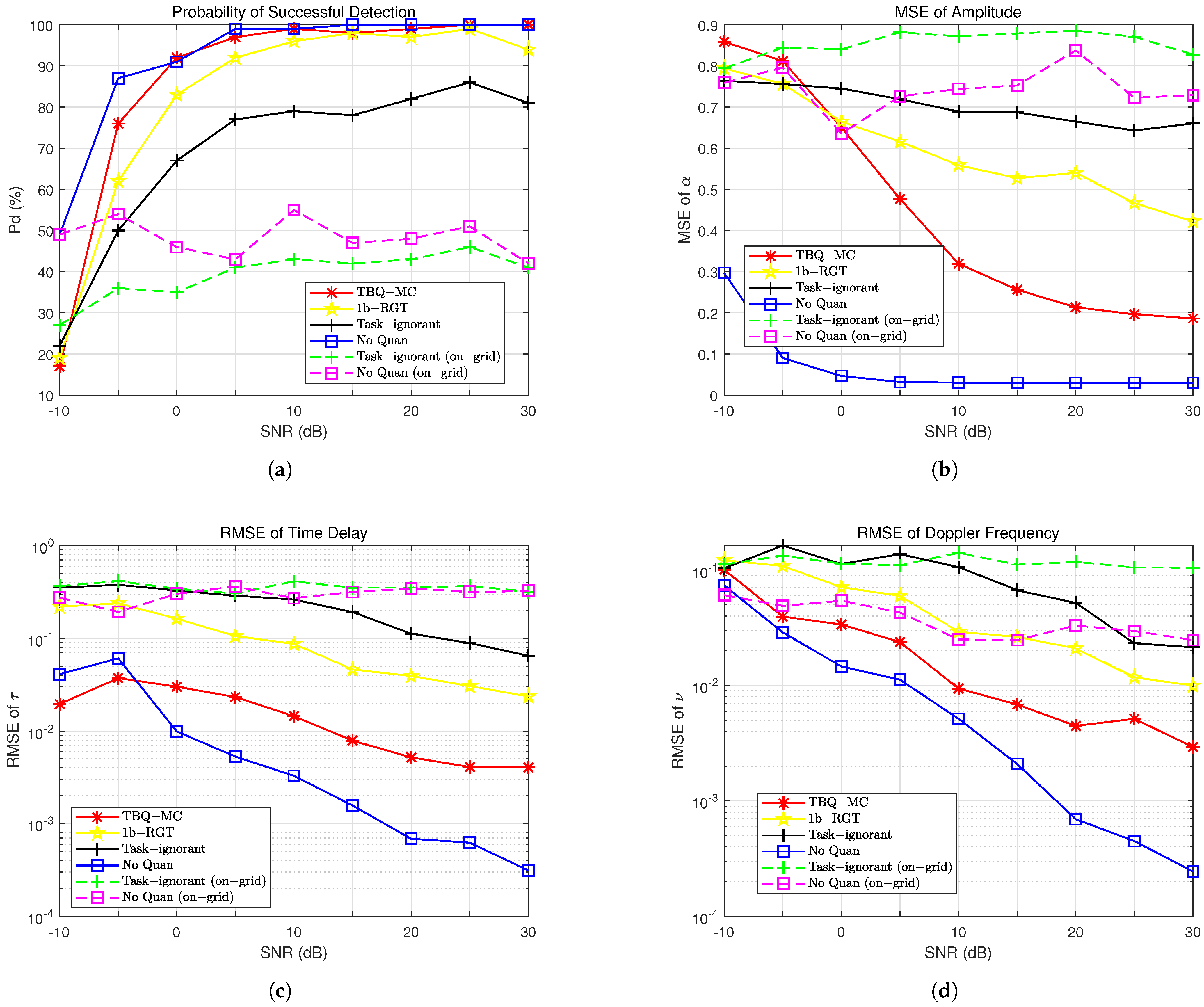
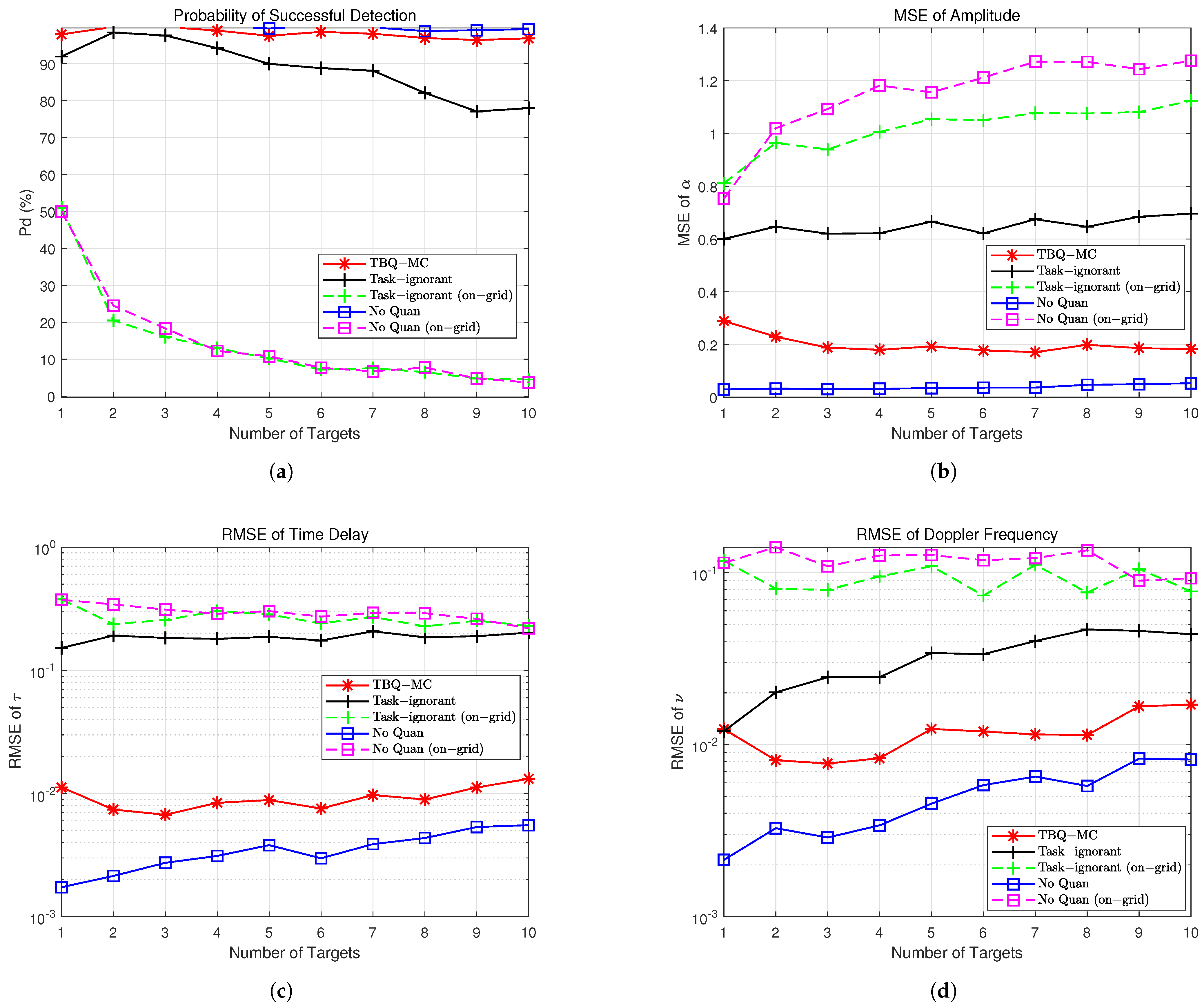
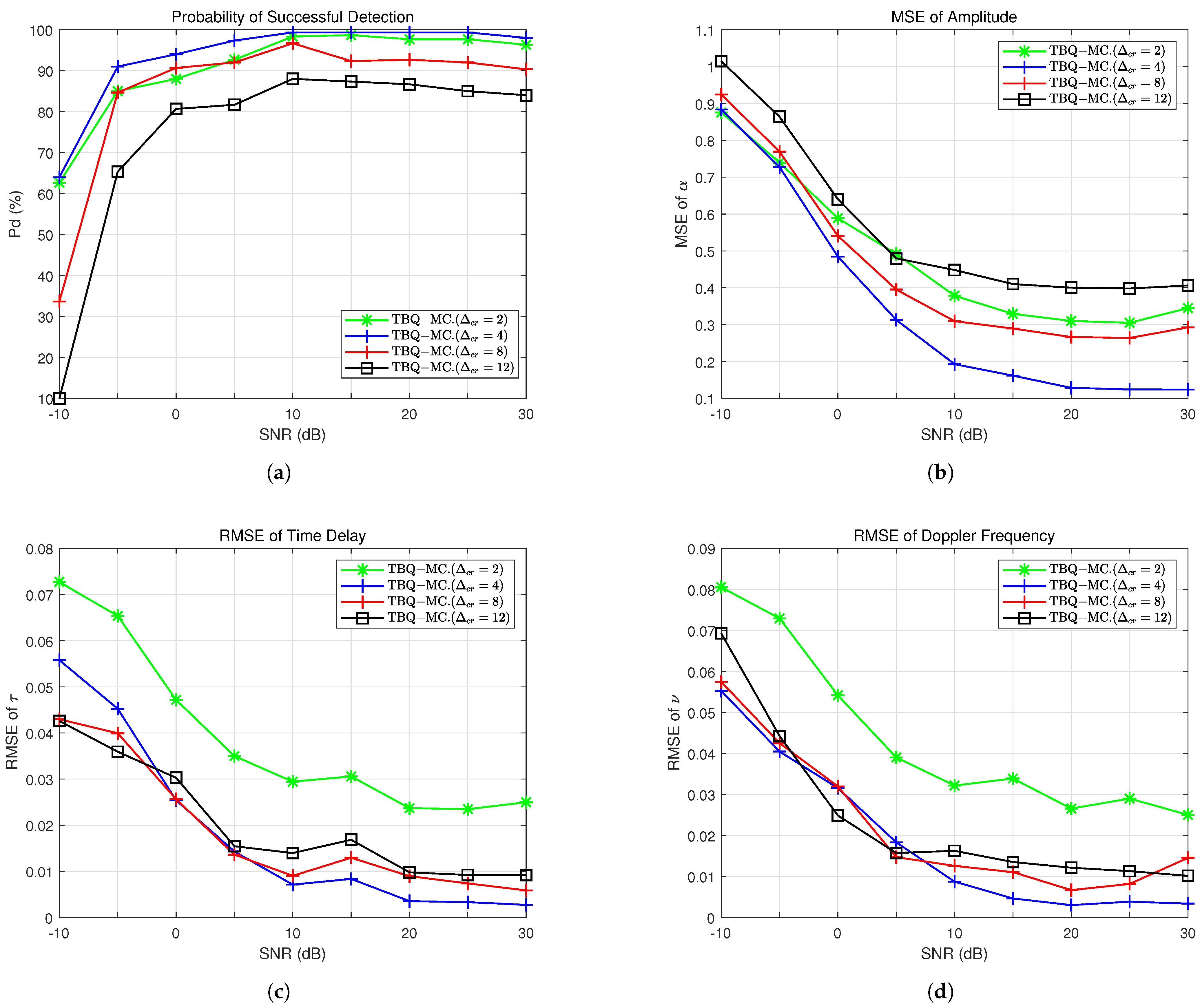
5.2. Recovery Performance

We evaluate the parameter estimation performance of the different methods using the following metrics:

(1)

Successful Detection Rate: A detection is considered successful when the estimation errors for both the delay and Doppler parameters are no more than one resolution bin.

(2)

MSE of Amplitude $\alpha$: The average MSEs for the magnitude and phase estimation of the target’s reflection coefficients.

(3)

RMSE of Time Delay $\tau$: The relative root MSE (RMSE) of the delay $\tau$, normalized to the time-delay Nyquist bin for successfully detected targets.

(4)

RMSE of Doppler Frequency $\nu$: The RMS of the Doppler frequency $\nu$, normalized to the Doppler frequency Nyquist bin for successfully detected targets.

Because the RMSE metric is sensitive to outliers, we present the estimation accuracy of the target delay and Doppler frequencies in two aspects: the successful detection rate, and the RMS values for targets that are successfully detected. The MSE of the amplitude $\alpha$ illustrates the estimation accuracy of the targets’ reflection coefficients.

We first evaluate the recovery performance of the six mentioned recovery methods versus the SNR using a given bit budget of $L=2NQ$. We consider a scenario with $K=1$ target. The compression ratio of TBQ-MC system is set to ${\mathsf{\Delta }}_{cr}=4$, with a total number of samples $MQ=1800$. The probability of successful detection, average MSE of the amplitude, and average RMSE of the delays and Doppler frequencies are shown in Figure 2a–d, respectively.

As shown in Figure 2a, for SNRs above 0 dB, the proposed TBQ-MC method achieves detection performance comparable to the “No Quan” method, which operates with infinite resolution; in addition, it clearly outperforms the “Task-ignorant” method operating with the same bit budget. However, TBQ-MC experiences a noticeable performance degradation for SNRs below 0 dB. This decline is primarily due to the reduced number of samples, which negatively affects performance at low SNRs. It is well known in the CS literature that measurement compression significantly impacts SNR, leading to degradation of recovery performance in a phenomenon referred to as noise folding. While the compression in the TBQ-MC method saves bits for each sample, the noise folding induced by subsampling negatively impacts the estimation performance, especially at low SNRs. It is notable that the “1b-RGT” method adopts random time-varying thresholds in comparison to the “Task-ignorant” method, leading to a notable improvement in terms of detection performance, albeit slightly worse than that of TBQ-MC. Additionally, the other two methods, which rely on the on-grid recovery approach, both fail to achieve acceptable detection performance. This is because on-grid methods approximate parameters to the nearest grid points, introducing additional errors due to grid mismatch.

As shown in Figure 2b, both TBQ-MC and the “No Quan” approach exhibit a noticeable decrease in amplitude estimation errors as SNR increases. Similarly, the amplitude estimation error of the “1b-RGT” method decreases gradually as the SNR increases. In contrast, the other three methods maintain nearly consistent estimation errors for the amplitude across different SNR levels. Figure 2c,d illustrates the average RMSEs of the delays and Doppler frequencies. As the figure shows, the estimation errors of our method are only slightly worse than those of the “No Quan” method, particularly at high SNRs. The performance of the “1b-RGT” method shows limited improvement as the SNR increases, although it is slightly better than that of the “Task-ignorant” method. The two methods using the on-grid approach exhibit consistently higher estimation errors due to the effects of grid mismatch.

Next, we investigate the estimation performance for varying numbers of targets, with the SNR fixed at 10 dB and a given bit budget $L=4NQ$. The results are shown in Figure 3.

As illustrated in Figure 3a, the probability of successful detection for both the TBQ-MC method and the “No Quan” method remains nearly constant as the number of targets increases, with both achieving near-perfect detection rates. In contrast, the detection performance of the “Task-ignorant” method degrades significantly as the number of targets increases. Moreover, the two on-grid methods fail to resolve the targets effectively as the number of targets grows. This is primarily due to the significant impact of grid mismatch on target detection, especially when dealing with a large number of targets. The MSE of the amplitude, as shown in Figure 3b, follows the same trend as in Figure 3a, with the TBQ-MC method and the “No Quan” method outperforming the others in terms of amplitude estimation accuracy. The curves in Figure 3c,d indicate that both the “No Quan” and TBQ-MC methods achieve satisfactory accuracy in estimating the time delays and Doppler frequencies. In contrast, the two on-grid recovery methods exhibit significant performance gaps due to grid mismatch.

Next, we evaluate the recovery performance of the TBQ-MC method with different total numbers of bits and with the compression ratio fixed at ${\mathsf{\Delta }}_{cr}=4$. We exclude the two on-grid methods from this simulation, as they have already proven to be inefficient for gridless parameter estimation. As illustrated in Figure 4, the recovery performance of both the proposed TBQ-MC method and the “Task-ignorant” method show consistent improvement with an increasing number of bits. Notably, the TBQ-MC method outperforms the “Task-ignorant” method across all performance metrics and closely approaches the performance of the “No Quan” system. This demonstrates the effectiveness of the TBQ-MC method in minimizing quantization effects while achieving high recovery accuracy, highlighting its superiority in handling quantized data.

Finally, we investigate the recovery performance of the TBQ-MC method for different compression ratios. The total number of bits is fixed at $4NQ$ = 28,800. We set four distinct compression ratios, i.e., ${\mathsf{\Delta }}_{cr}$, and compare the recovery performance of the TBQ-MC methods across these settings.

As shown in Figure 5a, the TBQ-MC receivers with ${\mathsf{\Delta }}_{cr}=4$ and ${\mathsf{\Delta }}_{cr}=2$ exhibit similar detection performance, with only a small gap between them. Both methods outperform the others. We observe that the TBQ-MC receiver with a larger compression ratio ${\mathsf{\Delta }}_{cr}=12$ saves more bits per sample within the given bit budget, which is expected to reduce quantization distortion. However, excessive compression leads to significant performance loss, especially at low SNRs, where noise folding becomes more pronounced. Conversely, while the receiver with a smaller compression ratio is less affected by compression artifacts, its advantages in reducing quantization distortion are relatively limited.

The amplitude recovery accuracy shown in Figure 5b demonstrates that the TBQ-MC receiver with ${\mathsf{\Delta }}_{cr}=4$ achieves the best performance, whereas the receiver with ${\mathsf{\Delta }}_{cr}=12$ exhibits the poorest performance. Figure 5c,d present the RMSEs for the delays and Doppler frequencies, respectively. The TBQ-MC receiver with ${\mathsf{\Delta }}_{cr}=4$ consistently demonstrates superior performance, while the receiver with ${\mathsf{\Delta }}_{cr}=2$ shows relatively higher error levels. This highlights the tradeoff between compression ratio and performance: higher compression ratios reduce the required number of bits, but introduce more compression-induced noise, which degrades performance; conversely, lower compression ratios are less affected by compression artifacts, but offer limited benefits in reducing quantization errors.

5.3. Summary

The enhanced performance of the TBQ-MC receiver can be attributed to two key design strategies:

• Sample Reduction with Subsampling: By employing a subsampling scheme to define the system task, it is possible to reduce the number of samples, allowing for increased bit depth per measurement while staying within the total bit budget constraint. This strategy minimizes quantization distortion by allocating more bits to each sample, resulting in higher precision and improved signal quality.
• Joint System Design Optimization: The second strategy involves a holistic design approach for the entire receiver system, considering the specific tasks and objectives of the system. This joint design ensures that all components work together efficiently, enhancing overall performance. By leveraging the interdependencies between various parts of the system, the design is optimized for the intended application and operational requirements, leading to better results.

By integrating these two strategies, the TBQ-MC receiver not only reduces quantization errors but also optimizes its architecture for the best possible performance tailored to its designated tasks.

It is important to note that selecting an appropriate compression ratio for the TBQ-MC system is crucial, as the receiver’s performance varies significantly depending on the chosen compression ratio. The optimal compression ratio strikes a balance between quantization distortion and noise folding effects. Additionally, the compression ratio directly impacts both system performance and hardware design complexity, as it influences the data volume and consequently the cost of the system.

Generally, sub-Nyquist sampling is accomplished by low-rate ADCs in conjunction with analog preprocessing. In our work, we propose a tunable HAD architecture designed to achieve subsampling, simultaneously optimizing the analog preprocessing, low-rate low-resolution ADCs, and digital filtering. The digital filtering component is specifically implemented to compensate for the quantization distortion resulting from the limited bit budget. This approach enhances the system’s performance; moreover, it offers a fresh perspective on the HAD structure’s functionality, showcasing its potential for being tailored to meet specific system tasks.

6. Conclusions

In this work, we proposed a bit-limited pulse–Doppler radar receiver by integrating subsampling and task-based quantization methods. We apply the HAD architecture to the pulse–Doppler radar receiver while jointly optimizing the analog component, low-rate ADCs, and digital processing component within the constraint of a fixed bit budget. The atomic norm minimization method is utilized to recover the complete parameter matrix from the compressed task vector. Simulation results demonstrate the effectiveness of the proposed TBQ-MC receiver; specifically, the TBQ-MC receiver outperforms conventional processing methods with the same bit budget, achieving higher successful detection rates and improved parameter estimation accuracy. Future work will extend the proposed framework to more complex radar environments such as cluttered environments in order to further enhance the receiver’s performance in real-world conditions.

References

1. Walden, R. Analog-to-digital converter survey and analysis. IEEE J. Sel. Areas Commun. 1999, 17, 539–550. [Google Scholar] [CrossRef]
2. Lee, H.S.; Sodini, C.G. Analog-to-Digital Converters: Digitizing the Analog World. Proc. IEEE 2008, 96, 323–334. [Google Scholar] [CrossRef]
3. Kaushik, A.; Tsinos, C.; Vlachos, E.; Thompson, J. Energy Efficient ADC Bit Allocation and Hybrid Combining for Millimeter Wave MIMO Systems. In Proceedings of the 2019 IEEE Global Communications Conference, Waikoloa, HI, USA, 9–13 December 2019; pp. 1–6. [Google Scholar] [CrossRef]
4. Candès, E.J.; Wakin, M.B. An Introduction To Compressive Sampling. IEEE Signal Process. Mag. 2008, 25, 21–30. [Google Scholar] [CrossRef]
5. Mishali, M.; Eldar, Y.C.; Elron, A.J. Xampling: Signal Acquisition and Processing in Union of Subspaces. IEEE Trans. Signal Process. 2011, 59, 4719–4734. [Google Scholar] [CrossRef]
6. Cohen, D.; Eldar, Y.C. Reduced time-on-target in pulse-Doppler radar: Slow time domain compressed sensing. In Proceedings of the 2016 IEEE Radar Conference (RadarConf), Philadelphia, PA, USA, 2–6 May 2016; pp. 1–4. [Google Scholar] [CrossRef]
7. Xi, F.; Chen, S.; Liu, Z. Quadrature Compressive Sampling for Radar Signals. IEEE Trans. Signal Process. 2014, 62, 2787–2802. [Google Scholar] [CrossRef]
8. Liu, C.; Xi, F.; Chen, S.; Zhang, Y.D.; Liu, Z. Pulse-Doppler signal processing with quadrature compressive sampling. IEEE Trans. Aerosp. Electron. Syst. 2015, 51, 1217–1230. [Google Scholar] [CrossRef]
9. Bar-Ilan, O.; Eldar, Y.C. Sub-Nyquist Radar via Doppler Focusing. IEEE Trans. Signal Process. 2014, 62, 1796–1811. [Google Scholar] [CrossRef]
10. Cohen, D.; Cohen, D.; Eldar, Y.C.; Haimovich, A.M. SUMMeR: Sub-Nyquist MIMO Radar. IEEE Trans. Signal Process. 2018, 66, 4315–4330. [Google Scholar] [CrossRef]
11. Masry, E. Random sampling of deterministic signals: Statistical analysis of Fourier transform estimates. IEEE Trans. Signal Process. 2006, 54, 1750–1761. [Google Scholar] [CrossRef]
12. Shlezinger, N.; Eldar, Y.C.; Rodrigues, M.R.D. Hardware-Limited Task-Based Quantization. IEEE Trans. Signal Process. 2019, 67, 5223–5238. [Google Scholar] [CrossRef]
13. Shlezinger, N.; Eldar, Y.C. Task-Based Quantization with Application to MIMO Receivers. arXiv 2020, arXiv:2002.04290. [Google Scholar] [CrossRef]
14. Shlezinger, N.; Eldar, Y.C.; Rodrigues, M.R.D. Asymptotic Task-Based Quantization with Application to Massive MIMO. IEEE Trans. Signal Process. 2019, 67, 3995–4012. [Google Scholar] [CrossRef]
15. Shlezinger, N.; van Sloun, R.J.G.; Huijben, I.A.M.; Tsintsadze, G.; Eldar, Y.C. Learning Task-Based Analog-to-Digital Conversion for MIMO Receivers. In Proceedings of the ICASSP 2020—2020 IEEE International Conference on Acoustics, Speech and Signal Processing (ICASSP), Virtual, 4–9 May 2020; pp. 9125–9129. [Google Scholar] [CrossRef]
16. Wang, H.; Shlezinger, N.; Eldar, Y.C.; Jin, S.; Imani, M.F.; Yoo, I.; Smith, D.R. Dynamic Metasurface Antennas for MIMO-OFDM Receivers With Bit-Limited ADCs. IEEE Trans. Commun. 2021, 69, 2643–2659. [Google Scholar] [CrossRef]
17. Xi, F.; Shlezinger, N.; Eldar, Y.C. BiLiMO: Bit-Limited MIMO Radar via Task-Based Quantization. IEEE Trans. Signal Process. 2021, 69, 6267–6282. [Google Scholar] [CrossRef]
18. Xi, F.; Shlezinger, N.; Eldar, Y.C. Hybrid Analog-Digital MIMO Radar Receivers with Bit-Limited ADCs. In Proceedings of the ICASSP 2021—2021 IEEE International Conference on Acoustics, Speech and Signal Processing (ICASSP), Toronto, ON, Canada, 6–11 June 2021; pp. 4405–4409. [Google Scholar] [CrossRef]
19. Zirtiloglu, T.; Shlezinger, N.; Eldar, Y.C.; Tugce Yazicigil, R. Power-Efficient Hybrid MIMO Receiver with Task-Specific Beamforming using Low-Resolution ADCs. In Proceedings of the 2022 IEEE International Conference on Acoustics, Speech and Signal Processing (ICASSP), Singapore, 22–27 May 2022; pp. 5338–5342. [Google Scholar] [CrossRef]
20. Wang, Y.; Xi, F.; Chen, S.; Liu, Z. Bit-Limited Sub-Nyquist Pulse-Doppler Radar. IEEE Trans. Aerosp. Electron. Syst. 2024, 1–16. [Google Scholar] [CrossRef]
21. Yoo, J.; Turnes, C.; Nakamura, E.B.; Le, C.K.; Becker, S.; Sovero, E.A.; Wakin, M.B.; Grant, M.C.; Romberg, J.; Emami-Neyestanak, A.; et al. A Compressed Sensing Parameter Extraction Platform for Radar Pulse Signal Acquisition. IEEE J. Emerg. Sel. Top. Circuits Syst. 2012, 2, 626–638. [Google Scholar] [CrossRef]
22. Chi, Y.; Pezeshki, A.; Scharf, L.; Calderbank, R. Sensitivity to basis mismatch in compressed sensing. In Proceedings of the 2010 IEEE International Conference on Acoustics, Speech and Signal Processing, Dallas, TX, USA, 14–19 March 2010; pp. 3930–3933. [Google Scholar] [CrossRef]
23. Candès, E.J.; Plan, Y. Matrix Completion with Noise. Proc. IEEE 2010, 98, 925–936. [Google Scholar] [CrossRef]
24. Candès, E.J.; Plan, Y. Accurate low-rank matrix recovery from a small number of linear measurements. In Proceedings of the 2009 47th Annual Allerton Conference on Communication, Control, and Computing (Allerton), Monticello, IL, USA, 30 September–2 October 2009; pp. 1223–1230. [Google Scholar] [CrossRef]
25. Candès, E.; Li, X.; Ma, Y.; Wright, J. Robust principal component analysis: Recovering low-rank matrices from sparse errors. In Proceedings of the 2010 IEEE Sensor Array and Multichannel Signal Processing Workshop, Jerusalem, Israel, 4–7 October 2010; pp. 201–204. [Google Scholar] [CrossRef]
26. Candès, E.J.; Plan, Y. Tight Oracle Inequalities for Low-Rank Matrix Recovery From a Minimal Number of Noisy Random Measurements. IEEE Trans. Inf. Theory 2011, 57, 2342–2359. [Google Scholar] [CrossRef]
27. Xi, F.; Chen, S.; Liu, Z. Super-resolution delay-Doppler estimation for sub-Nyquist radar via atomic norm minimization. In Proceedings of the 2017 IEEE International Conference on Acoustics, Speech and Signal Processing (ICASSP), New Orleans, LA, USA, 5–9 March 2017; pp. 4326–4330. [Google Scholar] [CrossRef]
28. Xi, F.; Xiang, Y.; Chen, S.; Nehorai, A. Gridless Parameter Estimation for One-Bit MIMO Radar with Time-Varying Thresholds. IEEE Trans. Signal Process. 2020, 68, 1048–1063. [Google Scholar] [CrossRef]
29. Candès, E.J.; Recht, B. Exact Matrix Completion via Convex Optimization. Found. Comput. Math. 2009, 9, 717–772. [Google Scholar] [CrossRef]
30. Sun, S.; Bajwa, W.U.; Petropulu, A.P. MIMO-MC radar: A MIMO radar approach based on matrix completion. IEEE Trans. Aerosp. Electron. Syst. 2015, 51, 1839–1852. [Google Scholar] [CrossRef]
31. Boric-Lubecke, O.; Lubecke, V.M.; Droitcour, A.D.; Park, B.K.; Singh, A. Radar Principles. In Doppler Radar Physiological Sensing; John Wiley & Sons, Inc.: Hoboken, NJ, USA, 2016; pp. 21–38. [Google Scholar] [CrossRef]
32. Vaishampayan, V. Design of multiple description scalar quantizers. IEEE Trans. Inf. Theory 1993, 39, 821–834. [Google Scholar] [CrossRef]
33. Boyd, S.; Parikh, N.; Chu, E.; Peleato, B.; Eckstein, J. Distributed Optimization and Statistical Learning via the Alternating Direction Method of Multipliers. Found. Trends Mach. Learn. 2011, 3, 1–122. [Google Scholar] [CrossRef]
34. Kay, S.; Nekovei, R. An efficient two-dimensional frequency estimator. IEEE Trans. Acoust. Speech, Signal Process. 1990, 38, 1807–1809. [Google Scholar] [CrossRef]
35. Hua, Y. Estimating two-dimensional frequencies by matrix enhancement and matrix pencil. IEEE Trans. Signal Process. 1992, 40, 2267–2280. [Google Scholar] [CrossRef]
36. Tang, W.G.; Jiang, H.; Zhang, Q. Admm for Gridless Dod and Doa Estimation in Bistatic Mimo Radar Based on Decoupled Atomic Norm Minimization with One Snapshot. In Proceedings of the 2019 IEEE Global Conference on Signal and Information Processing (GlobalSIP), Ottawa, ON, Canada, 11–14 November 2019; pp. 1–5. [Google Scholar] [CrossRef]
Figure 1. The proposed task-based quantizer via matrix completion (TBQ-MC) architecture.
Remotesensing 17 00982 g001
Figure 2. Recovery performance of different methods versus SNR ( K = 1 , bit budget of 2 N Q = 14,400): (a) successful detection rate, (b) MSE of amplitude α , (c) RMSE of time delay τ , (d) RMSE of Doppler frequency ν .
Remotesensing 17 00982 g002
Figure 3. Recovery performance of different methods versus number of targets (SNR = 10 dB, bit budget of 4 N Q = 28,800): (a) successful detection rate, (b) MSE of amplitude α , (c) RMSE of time delay τ , (d) RMSE of Doppler frequency ν .
Remotesensing 17 00982 g003
Figure 4. Recovery performance of different methods versus total number of bits ( K = 3 , SNR = 10 dB): (a) successful detection rate, (b) MSE of amplitude α , (c) RMSE of time delay τ , (d) RMSE of Doppler frequency ν .
Remotesensing 17 00982 g004
Figure 5. Recovery performance of different Δ c r versus SNR ( K = 3 , bit budget of 4 N Q = 28,800): (a) successful detection rate, (b) MSE of amplitude α , (c) RMSE of time delay τ , (d) RMSE of Doppler frequency ν .
Remotesensing 17 00982 g005
Disclaimer/Publisher’s Note: The statements, opinions and data contained in all publications are solely those of the individual author(s) and contributor(s) and not of MDPI and/or the editor(s). MDPI and/or the editor(s) disclaim responsibility for any injury to people or property resulting from any ideas, methods, instructions or products referred to in the content.