
Can Stereoscopic Density Replace Planar Density for Forest Aboveground Biomass Estimation? A Case Study Using Airborne LiDAR and Landsat Data in Daxing’anling, China

 ,
, 
Abstract
:1. Introduction
2. Materials and Methods
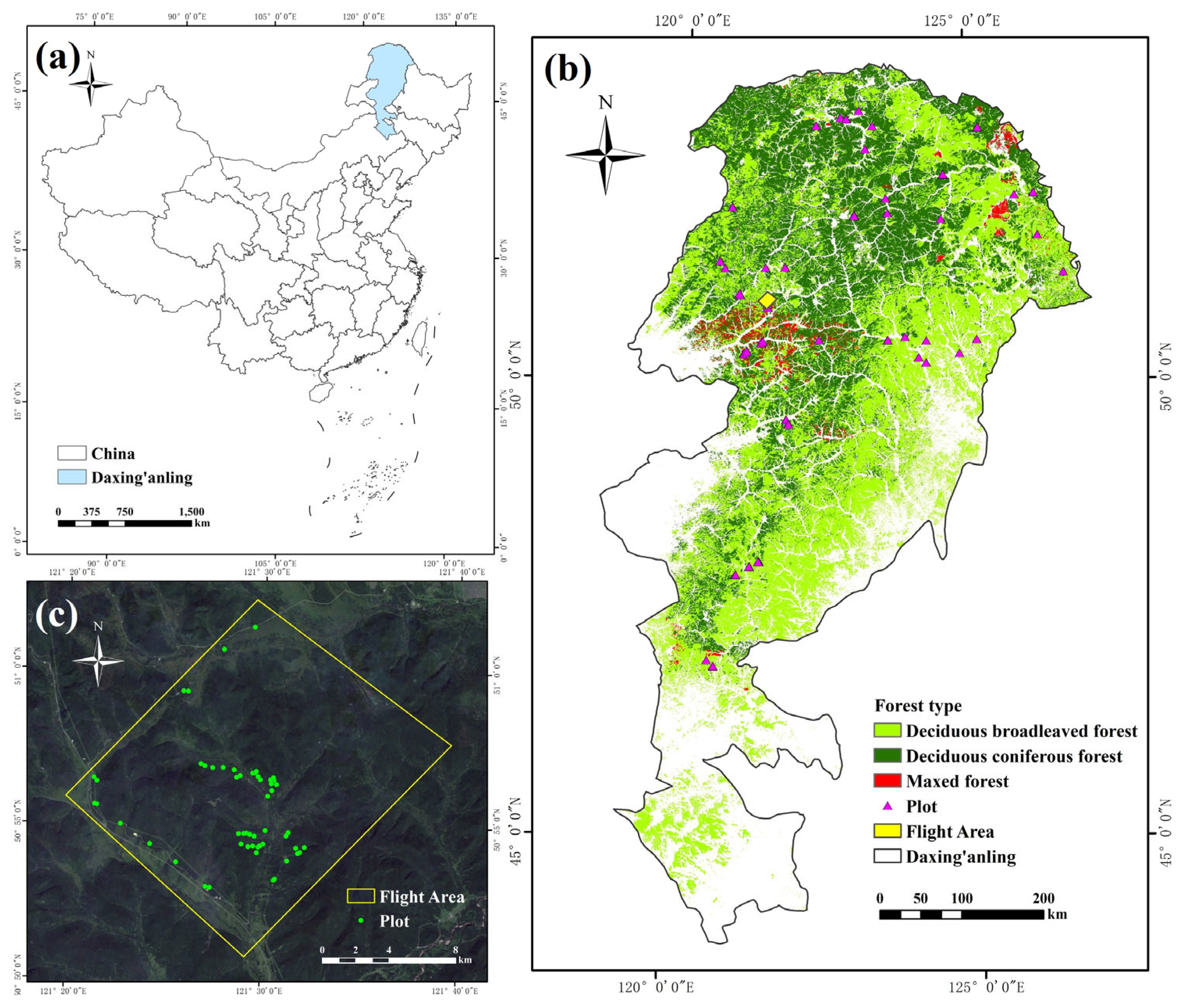
2.1. Study Area
2.2. LiDAR Data
2.3. Field Data
2.4. Landsat5 TM Data
2.5. Auxiliary Data
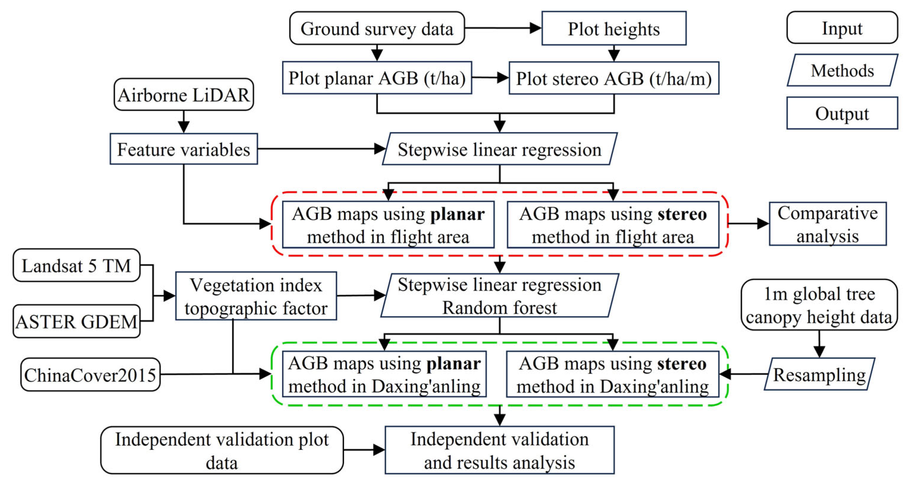
2.6. Methods
2.6.1. AGB Monitoring Model Based on Planar Density × Area for the Plot Scale
2.6.2. AGB Monitoring Model Based on Stereo Density × Volume for the Plot Scale
2.6.3. Planar and Stereo AGB Estimation with Landsat Data in the Daxing’anling
3. Results
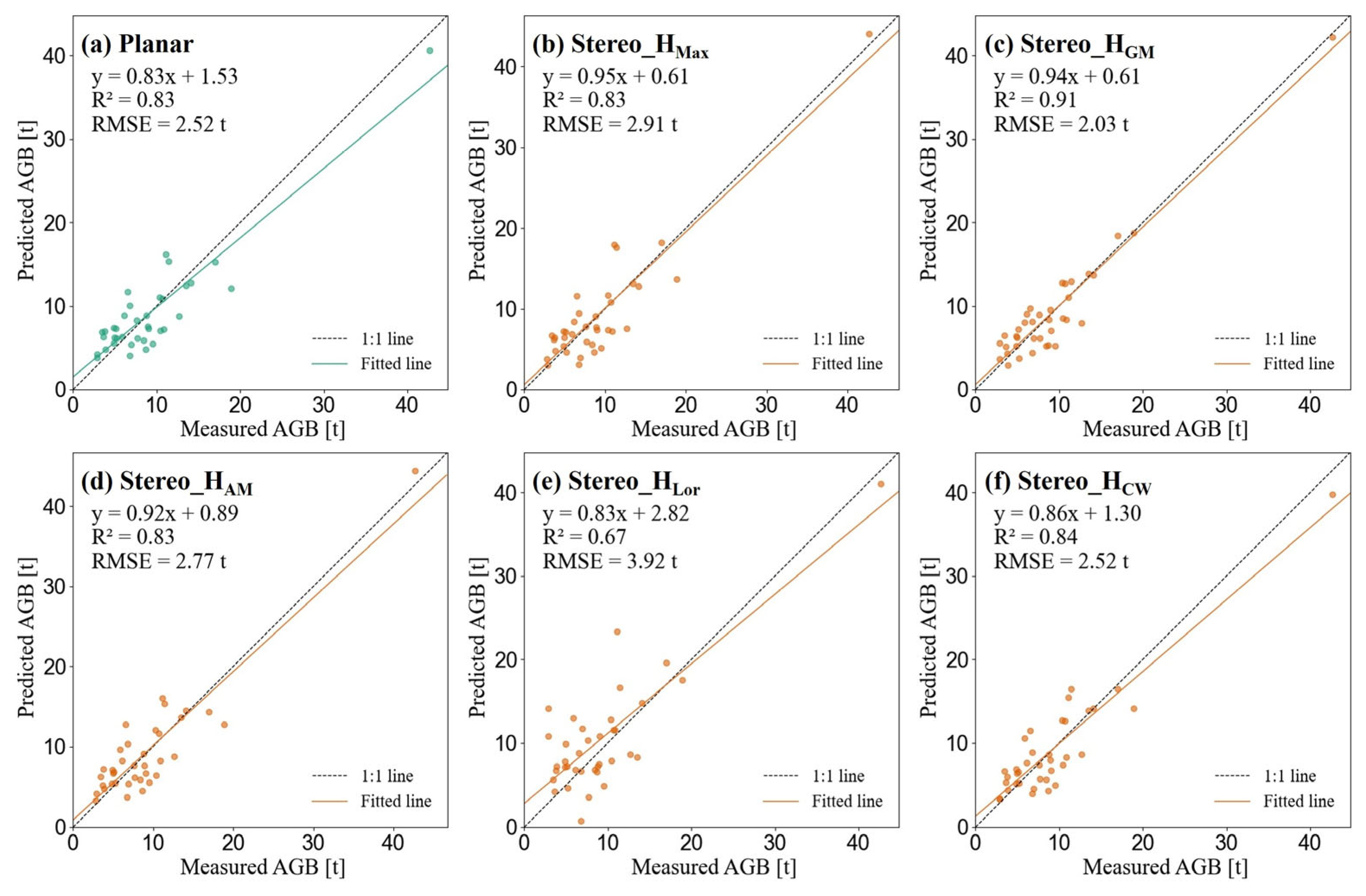
3.1. AGB Monitoring Results Based on Planar and Stereo Methods at the Plot Scale
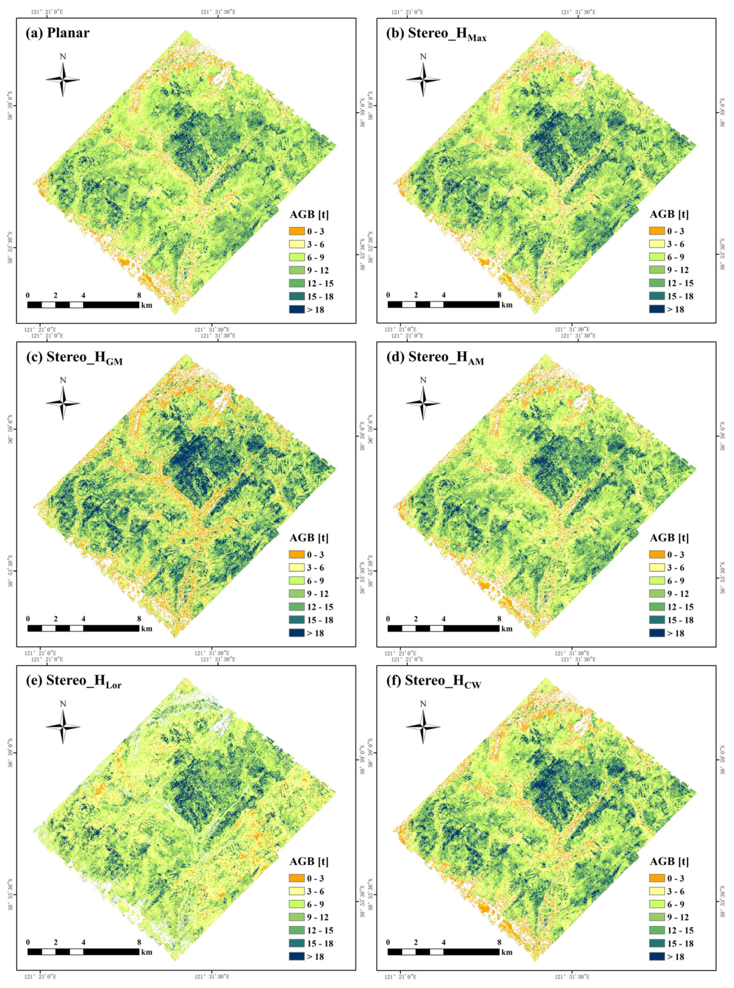
3.2. AGB Density Estimation Model at the Flight Area Scale
3.3. AGB Estimation Results in the Daxing’anling
4. Discussion
4.1. Applicability of the AGB Stereo Method on Airborne LiDAR Data
4.2. Applicability of the AGB Stereo Method at the Regional Scale
4.3. Limitations
5. Conclusions
Author Contributions
Funding
Data Availability Statement
Acknowledgments
Conflicts of Interest
References
- Zeng, Y.; Schaepman, M.E.; Wu, B.; Clevers, J.G.P.W.; Bregt, A.K. Quantitative Forest Canopy Structure Assessment Using an Inverted Geometric-optical Model and Up-scaling. Int. J. Remote Sens. 2009, 30, 1385–1406. [Google Scholar] [CrossRef]
- Cao, M.; Woodward, F.I.N. Net Primary and Ecosystem Production and Carbon Stocks of Terrestrial Ecosystems and Their Responses to Climate Change. Glob. Change Biol. 1998, 4, 185–198. [Google Scholar] [CrossRef]
- Zhang, R.; Zhou, X.; Ouyang, Z.; Avitabile, V.; Qi, J.; Chen, J.; Giannico, V. Estimating Aboveground Biomass in Subtropical Forests of China by Integrating Multisource Remote Sensing and Ground Data. Remote Sens. Environ. 2019, 232, 111341. [Google Scholar] [CrossRef]
- Tuominen, S.; Eerikinen, K.; Schibalski, A.; Haakana, M.; Lehtonen, A. Mapping Biomass Variables with a Multi-Source Forest Inventory Technique. Silva Fenn. 2010, 44, 109–119. [Google Scholar] [CrossRef]
- Xue, B.-L.; Guo, Q.; Hu, T.; Wang, G.; Wang, Y.; Tao, S.; Su, Y.; Liu, J.; Zhao, X. Evaluation of Modeled Global Vegetation Carbon Dynamics: Analysis Based on Global Carbon Flux and above-Ground Biomass Data. Ecol. Model. 2017, 355, 84–96. [Google Scholar] [CrossRef]
- Næsset, E.; Ørka, H.O.; Solberg, S.; Bollandsås, O.M.; Hansen, E.H.; Mauya, E.; Zahabu, E.; Malimbwi, R.; Chamuya, N.; Olsson, H.; et al. Mapping and Estimating Forest Area and Aboveground Biomass in Miombo Woodlands in Tanzania Using Data from Airborne Laser Scanning, TanDEM-X, RapidEye, and Global Forest Maps: A Comparison of Estimated Precision. Remote Sens. Environ. 2016, 175, 282–300. [Google Scholar] [CrossRef]
- Huang, H.; Liu, C.; Wang, X.; Zhou, X.; Gong, P. Integration of Multi-Resource Remotely Sensed Data and Allometric Models for Forest Aboveground Biomass Estimation in China. Remote Sens. Environ. 2019, 221, 225–234. [Google Scholar] [CrossRef]
- Dube, T.; Mutanga, O. Evaluating the Utility of the Medium-Spatial Resolution Landsat 8 Multispectral Sensor in Quantifying Aboveground Biomass in uMgeni Catchment, South Africa. ISPRS J. Photogramm. Remote Sens. 2015, 101, 36–46. [Google Scholar] [CrossRef]
- Ou, G.; Lv, Y.; Xu, H.; Wang, G. Improving Forest Aboveground Biomass Estimation of Pinus Densata Forest in Yunnan of Southwest China by Spatial Regression Using Landsat 8 Images. Remote Sens. 2019, 11, 2750. [Google Scholar] [CrossRef]
- Houghton, R.A.; Hall, F.; Goetz, S.J. Importance of Biomass in the Global Carbon Cycle. J. Geophys. Res. Biogeosci. 2009, 114, G00E03. [Google Scholar] [CrossRef]
- Rodríguez-Veiga, P.; Wheeler, J.; Louis, V.; Tansey, K.; Balzter, H. Quantifying Forest Biomass Carbon Stocks from Space. Curr. For. Rep. 2017, 3, 1–18. [Google Scholar] [CrossRef]
- Kerebeh, H.; Forkel, M.; Zewdie, W. Above Ground Biomass Estimation in the Upper Blue Nile Basin Forests, North-Western Ethiopia. Environ. Syst. Res. 2024, 13, 48. [Google Scholar] [CrossRef]
- Zhu, X.; Liu, D. Improving Forest Aboveground Biomass Estimation Using Seasonal Landsat NDVI Time-Series. ISPRS J. Photogramm. Remote Sens. 2015, 102, 222–231. [Google Scholar] [CrossRef]
- Talebiesfandarani, S.; Shamsoddini, A. Global-Scale Biomass Estimation Based on Machine Learning and Deep Learning Methods. Remote Sens. Appl. Soc. Environ. 2022, 28, 100868. [Google Scholar] [CrossRef]
- Marshak, C.; Simard, M.; Duncanson, L.; Silva, C.A.; Denbina, M.; Liao, T.-H.; Fatoyinbo, L.; Moussavou, G.; Armston, J. Regional Tropical Aboveground Biomass Mapping with L-Band Repeat-Pass Interferometric Radar, Sparse Lidar, and Multiscale Superpixels. Remote Sens. 2020, 12, 2048. [Google Scholar] [CrossRef]
- Rodríguez-Veiga, P.; Barbosa-Herrera, A.P.; Barreto-Silva, J.S.; Bispo, P.C.; Cabrera, E.; Capachero, C.; Galindo, G.; Gou, Y.; Moreno, L.M.; Louis, V.; et al. Mapping the Spatial Distribution of Colombia’s Forest Aboveground Biomass Using SAR and Optical Data. Int. Arch. Photogramm. Remote Sens. Spat. Inf. Sci. 2019, 42, 57–60. [Google Scholar] [CrossRef]
- Tebaldini, S.; d’Alessandro, M.M.; Ulander, L.M.H.; Bennet, P.; Gustavsson, A.; Coccia, A.; Macedo, K.; Disney, M.; Wilkes, P.; Spors, H.-J.; et al. TomoSense: A Unique 3D Dataset over Temperate Forest Combining Multi-Frequency Mono- and Bi-Static Tomographic SAR with Terrestrial, UAV and Airborne Lidar, and in-Situ Forest Census. Remote Sens. Environ. 2023, 290, 113532. [Google Scholar] [CrossRef]
- Ni, W.; Ranson, K.J.; Zhang, Z.; Sun, G. Features of Point Clouds Synthesized from Multi-View ALOS/PRISM Data and Comparisons with LiDAR Data in Forested Areas. Remote Sens. Environ. 2014, 149, 47–57. [Google Scholar] [CrossRef]
- Jiang, X.; Li, G.; Lu, D.; Chen, E.; Wei, X. Stratification-Based Forest Aboveground Biomass Estimation in a Subtropical Region Using Airborne Lidar Data. Remote Sens. 2020, 12, 1101. [Google Scholar] [CrossRef]
- Brede, B.; Terryn, L.; Barbier, N.; Bartholomeus, H.M.; Bartolo, R.; Calders, K.; Derroire, G.; Krishna Moorthy, S.M.; Lau, A.; Levick, S.R.; et al. Non-Destructive Estimation of Individual Tree Biomass: Allometric Models, Terrestrial and UAV Laser Scanning. Remote Sens. Environ. 2022, 280, 113180. [Google Scholar] [CrossRef]
- Beland, M.; Parker, G.; Sparrow, B.; Harding, D.; Chasmer, L.; Phinn, S.; Antonarakis, A.; Strahler, A. On Promoting the Use of Lidar Systems in Forest Ecosystem Research. For. Ecol. Manag. 2019, 450, 117484. [Google Scholar] [CrossRef]
- Campbell, M.J.; Dennison, P.E.; Kerr, K.L.; Brewer, S.C.; Anderegg, W.R.L. Scaled Biomass Estimation in Woodland Ecosystems: Testing the Individual and Combined Capacities of Satellite Multispectral and Lidar Data. Remote Sens. Environ. 2021, 262, 112511. [Google Scholar] [CrossRef]
- Meng, G.; Zhao, D.; Xu, C.; Chen, J.; Li, X.; Zheng, Z.; Zeng, Y. Forest aboveground biomass estimation combining ICESat-2 and GEDI spaceborne LiDAR data. Natl. Remote Sens. Bull. 2022, 28, 1632–1647. [Google Scholar] [CrossRef]
- Liang, M.; Duncanson, L.; Silva, J.A.; Sedano, F. Quantifying Aboveground Biomass Dynamics from Charcoal Degradation in Mozambique Using GEDI Lidar and Landsat. Remote Sens. Environ. 2023, 284, 113367. [Google Scholar] [CrossRef]
- Meng, S.; Liu, Q.; Zhou, G.; Jia, Q.; Zhuang, H.; Zhou, H. Aboveground Tree Additive Biomass Equations for Two Dominant Deciduous Tree Species in Daxing’anling, Northernmost China. J. For. Res. 2017, 22, 233–240. [Google Scholar] [CrossRef]
- Meng, S.; Jia, Q.; Liu, Q.; Zhou, G.; Wang, H.; Yu, J. Aboveground Biomass Allocation and Additive Allometric Models for Natural Larix Gmelinii in the Western Daxing’anling Mountains, Northeastern China. Forests 2019, 10, 150. [Google Scholar] [CrossRef]
- Liu, K.; Wang, J.; Zeng, W.; Song, J. Comparison and Evaluation of Three Methods for Estimating Forest above Ground Biomass Using TM and GLAS Data. Remote Sens. 2017, 9, 341. [Google Scholar] [CrossRef]
- Wang, L.; Ju, Y.; Ji, Y.; Marino, A.; Zhang, W.; Jing, Q. Estimation of Forest Above-Ground Biomass in the Study Area of Greater Khingan Ecological Station with Integration of Airborne LiDAR, Landsat 8 OLI, and Hyperspectral Remote Sensing Data. Forests 2024, 15, 1861. [Google Scholar] [CrossRef]
- Asner, G.P. Tropical Forest Carbon Assessment: Integrating Satellite and Airborne Mapping Approaches. Environ. Res. Lett. 2009, 4, 034009. [Google Scholar] [CrossRef]
- Pang, Y.; Lefsky, M.; Andersen, H.-E.; Miller, M.E.; Sherrill, K. Validation of the ICEsat Vegetation Product Using Crown-Area-Weighted Mean Height Derived Using Crown Delineation with Discrete Return Lidar Data. Can. J. Remote Sens. 2008, 34, 471–484. [Google Scholar] [CrossRef]
- Huang, W.; Min, W.; Ding, J.; Liu, Y.; Hu, Y.; Ni, W.; Shen, H. Forest Height Mapping Using Inventory and Multi-Source Satellite Data over Hunan Province in Southern China. For. Ecosyst. 2022, 9, 100006. [Google Scholar] [CrossRef]
- Feng, Z.; Yu, X.; Chen, Y.; Puttonen, E.; Hakala, T.; Jiang, C.; Hyyppä, J. Feasibility of Using Ku-Band Helicopter-Borne Microwave Radar for Stem Volume and Biomass Estimation in Boreal Forest. Int. J. Appl. Earth Obs. Geoinf. 2024, 131, 103966. [Google Scholar] [CrossRef]
- Næsset, E. Predicting Forest Stand Characteristics with Airborne Scanning Laser Using a Practical Two-Stage Procedure and Field Data. Remote Sens. Environ. 2002, 80, 88–99. [Google Scholar] [CrossRef]
- D’Oliveira, M.V.N.; Reutebuch, S.E.; McGaughey, R.J.; Andersen, H.-E. Estimating Forest Biomass and Identifying Low-Intensity Logging Areas Using Airborne Scanning Lidar in Antimary State Forest, Acre State, Western Brazilian Amazon. Remote Sens. Environ. 2012, 124, 479–491. [Google Scholar] [CrossRef]
- Hansen, E.H.; Gobakken, T.; Bollandsås, O.M.; Zahabu, E.; Næsset, E. Modeling Aboveground Biomass in Dense Tropical Submontane Rainforest Using Airborne Laser Scanner Data. Remote Sens. 2015, 7, 788–807. [Google Scholar] [CrossRef]
- Wallis, C.I.B.; Homeier, J.; Peña, J.; Brandl, R.; Farwig, N.; Bendix, J. Modeling Tropical Montane Forest Biomass, Productivity and Canopy Traits with Multispectral Remote Sensing Data. Remote Sens. Environ. 2019, 225, 77–92. [Google Scholar] [CrossRef]
- Liu, Z.; Wu, Y.; Zhang, X.; Li, M.; Liu, C.; Li, W.; Fu, M.; Qin, S.; Fan, Q.; Luo, H.; et al. Comparison of Variable Extraction Methods Using Surface Field Data and Its Key Influencing Factors: A Case Study on Aboveground Biomass of Pinus densata Forest Using the Original Bands and Vegetation Indices of Landsat 8. Ecol. Indic. 2023, 157, 111307. [Google Scholar] [CrossRef]
- Xu, T.; Cao, L.; Shen, X.; She, G. Estimates of subtropical forest biomass based on airborne LiDAR and Landsat 8 OLI data. Chin. J. Plant Ecol. 2015, 39, 309–321. [Google Scholar] [CrossRef]
- Zhang, L.; Zhang, X.; Shao, Z.; Jiang, W.; Gao, H. Integrating Sentinel-1 and 2 with LiDAR Data to Estimate Aboveground Biomass of Subtropical Forests in Northeast Guangdong, China. Int. J. Digit. Earth 2023, 16, 158–182. [Google Scholar] [CrossRef]
- Wu, B.; Qian, J.; Zeng, Y. Land Cover Atlas of the People’s Republic of China (1:1,000,000); China Map Publishing House: Beijing, China, 2017; ISBN 978-7-5031-9823-6. [Google Scholar]
- Tolan, J.; Yang, H.-I.; Nosarzewski, B.; Couairon, G.; Vo, H.V.; Brandt, J.; Spore, J.; Majumdar, S.; Haziza, D.; Vamaraju, J.; et al. Very High Resolution Canopy Height Maps from RGB Imagery Using Self-Supervised Vision Transformer and Convolutional Decoder Trained on Aerial Lidar. Remote Sens. Environ. 2024, 300, 113888. [Google Scholar] [CrossRef]
- Fu, L.; Zhao, D.; Wu, B.; Xu, Z.; Zeng, Y. Variations in Forest Aboveground Biomass in Miyun Reservoir of Beijing over the Past Two Decades. J. Soils Sediments 2017, 17, 2080–2090. [Google Scholar] [CrossRef]
- Zhu, X.; Nie, S.; Wang, C.; Xi, X.; Lao, J.; Li, D. Consistency Analysis of Forest Height Retrievals between GEDI and ICESat-2. Remote Sens. Environ. 2022, 281, 113244. [Google Scholar] [CrossRef]
- Zhao, X.; Chen, J.M.; Zhang, Y.; Jiao, Z.; Liu, L.; Qiu, F.; Zang, J.; Cao, R. Global Mapping of Forest Clumping Index Based on GEDI Canopy Height and Complementary Data. ISPRS J. Photogramm. Remote Sens. 2024, 209, 1–16. [Google Scholar] [CrossRef]
- Wulder, M.A.; White, J.C.; Nelson, R.F.; Næsset, E.; Ørka, H.O.; Coops, N.C.; Hilker, T.; Bater, C.W.; Gobakken, T. Lidar Sampling for Large-Area Forest Characterization: A Review. Remote Sens. Environ. 2012, 121, 196–209. [Google Scholar] [CrossRef]
- Zhao, P.; Lu, D.; Wang, G.; Liu, L.; Li, D.; Zhu, J.; Yu, S. Forest Aboveground Biomass Estimation in Zhejiang Province Using the Integration of Landsat TM and ALOS PALSAR Data. Int. J. Appl. Earth Obs. Geoinf. 2016, 53, 1–15. [Google Scholar] [CrossRef]


| Feature Variable | Description |
|---|---|
| Canopy Closure (CC) | , the ratio of vegetation points in the first return to the total first return points. |
| Gap Fraction (GF) | , the ratio of ground points to total points. |
| Leaf Area Index (LAI) | , where ang is the average scan angle, GF is the gap fraction, and k is the extinction coefficient. |
| Canopy Relief Ratio (CRR) | , where mean, min, and max are height values of all points within a unit. |
| Accumulated Height Percentile (AIH) | Cumulative height of X% of points in a statistical unit based on normalized LiDAR data. |
| Interquartile Range of AIH (IQ) | Difference between the 75% and 25% percentiles of accumulated height. |
| Kurtosis | Coefficient of variation in Z-values within a statistical unit. |
| Coefficient of Variation (cv_z) | Measure of the flatness of Z-value distribution in a unit. |
| Density | Proportion of echoes in each of ten equally distributed height slices. |
| Median | Median Z-value of all points within a unit. |
| Max | Maximum Z-value of all points within a unit. |
| Min | Minimum Z-value of all points within a unit. |
| Mean | Mean Z-value of all points within a unit. |
| Height Percentile (Elev) | Height at the X% percentile of normalized LiDAR data within a unit. |
| Skewness | Symmetry of Z-value distribution in a unit. |
| Stddev | Standard deviation of Z-values within a unit. |
| Variance | Variance of Z-values within a unit. |
| Height Type | Calculation Formula |
|---|---|
| Maximum Height | |
| Geometric Mean Height | |
| Arithmetic Mean Height | |
| DBH-weighted Mean Height | |
| Canopy Area-weighted Mean Height |
| Vegetation Index | Calculation Formula |
|---|---|
| Normalized Difference Vegetation Index | |
| Enhanced Vegetation Index | |
| Soil-Adjusted Vegetation Index | |
| Simple Leaf Area Vegetation Index | |
| Simple Ratio Vegetation Index | |
| Difference Vegetation Index | |
| Mid-Infrared Vegetation Index | |
| Perpendicular Vegetation Index | |
| Transformed Normalized Difference Vegetation Index | |
| Red-Edge Vegetation Index | |
| Leaf Area Index | |
| Green Difference Vegetation Index | |
| Green Normalized Difference Vegetation Index | |
| Nonlinear Vegetation Index | |
| Red–Green Ratio Index |
| Methods | SLR | RF | |||||
|---|---|---|---|---|---|---|---|
| Metrics | Planar | Stereo_HAM | Stereo_HCW | Planar | Stereo_HAM | Stereo_HCW | |
| R2 | 0.44 | 0.50 | 0.50 | 0.46 | 0.52 | 0.52 | |
| RMSE | 25.37 t/ha | 1.99 t/ha/m | 1.78 t/ha/m | 24.87 t/ha | 1.95 t/ha/m | 1.74 t/ha/m | |
| rRMSE | 29.47% | 25.14% | 26.11% | 28.86% | 24.57% | 25.57% | |
Disclaimer/Publisher’s Note: The statements, opinions and data contained in all publications are solely those of the individual author(s) and contributor(s) and not of MDPI and/or the editor(s). MDPI and/or the editor(s) disclaim responsibility for any injury to people or property resulting from any ideas, methods, instructions or products referred to in the content. |
© 2025 by the authors. Licensee MDPI, Basel, Switzerland. This article is an open access article distributed under the terms and conditions of the Creative Commons Attribution (CC BY) license (https://creativecommons.org/licenses/by/4.0/).
Share and Cite
Mu, X.; Zhao, D.; Zheng, Z.; Xu, C.; Wu, J.; Zhao, P.; Li, X.; Pang, Y.; Zhao, Y.; An, T.; et al. Can Stereoscopic Density Replace Planar Density for Forest Aboveground Biomass Estimation? A Case Study Using Airborne LiDAR and Landsat Data in Daxing’anling, China. Remote Sens. 2025, 17, 1163. https://doi.org/10.3390/rs17071163
Mu X, Zhao D, Zheng Z, Xu C, Wu J, Zhao P, Li X, Pang Y, Zhao Y, An T, et al. Can Stereoscopic Density Replace Planar Density for Forest Aboveground Biomass Estimation? A Case Study Using Airborne LiDAR and Landsat Data in Daxing’anling, China. Remote Sensing. 2025; 17(7):1163. https://doi.org/10.3390/rs17071163
Chicago/Turabian StyleMu, Xuan, Dan Zhao, Zhaoju Zheng, Cong Xu, Jinchen Wu, Ping Zhao, Xiaomin Li, Yong Pang, Yujin Zhao, Tianyu An, and et al. 2025. "Can Stereoscopic Density Replace Planar Density for Forest Aboveground Biomass Estimation? A Case Study Using Airborne LiDAR and Landsat Data in Daxing’anling, China" Remote Sensing 17, no. 7: 1163. https://doi.org/10.3390/rs17071163
APA StyleMu, X., Zhao, D., Zheng, Z., Xu, C., Wu, J., Zhao, P., Li, X., Pang, Y., Zhao, Y., An, T., Zeng, Y., & Wu, B. (2025). Can Stereoscopic Density Replace Planar Density for Forest Aboveground Biomass Estimation? A Case Study Using Airborne LiDAR and Landsat Data in Daxing’anling, China. Remote Sensing, 17(7), 1163. https://doi.org/10.3390/rs17071163