Integrating Remote Sensing and Machine Learning for Actionable Flood Risk Assessment: Multi-Scenario Projection in the Ili River Basin in China Under Climate Change

Abstract

Climate change is leading to an increase in the frequency and intensity of flooding, making it necessary to consider future changes in flood risk management. In regions where ground-based observations are significantly restricted, the implementation of conventional risk assessment methodologies is always challenging. This study proposes an integrated remote sensing and machine learning approach for flood risk assessment in data-scarce regions. We extracted the historical inundation frequency using Sentinel-1 SAR and Landsat imagery from 2001 to 2023 and predicted flood susceptibility and inundation frequency using XGBoost, Random Forest (RF), and LightGBM models. The risk assessment framework systematically integrates hazard components (flood susceptibility and inundation frequency) with vulnerability factors (population, GDP, and land use) in two SSP-RCP scenarios. The results indicate that in the SSP2-RCP4.5 and SSP5-RCP8.5 scenarios, combined high- and very-high-flood-risk areas in the Ili River Basin in China (IRBC) are projected to reach 29.1% and 29.7% of the basin by 2050, respectively. In the short term, the contribution of inundation frequency to risk is predominant, while vulnerability factors, particularly population, contribute increasingly in the long term. This study demonstrates that integrating open geospatial data with machine learning enables actionable flood risk assessment, quantitatively supporting climate-resilient planning.

1. Introduction

Floods are the most widely distributed natural disaster globally with severe impacts. Between 2000 and 2019, flood events accounted for 44% of the global natural disaster occurrences, resulting in damage of USD 651 billion [1].

In the context of climate change, the impact of flooding has been steadily increasing. The Sixth Assessment Report of the IPCC (AR6) indicates that global warming will increase the probability of century-scale flood events between 30% and 50% under 1.5 °C warming scenarios [2]. This escalating threat is projected to drive population displacement, potentially leading to 216 million internal climate migrants by 2050, where flooding serves as a primary catalyst [3]. Asia is the most affected, absorbing 76% of the global flood-induced economic losses from 2020 to 2023 [4]. As one of the representative countries, China is facing growing conflicts between socio-economic development and increasing extreme hydrological events [5,6]. Traditional flood defense systems struggle to accommodate the expanding agricultural activities, infrastructure networks, and population exposure in floodplains [7]. In order to support governmental decision-making, climate change-oriented assessments of future flood risk trends are imperative.

Flood risk is generally defined as a product of hazard, exposure, and vulnerability [8,9]. Hazard represents the intensity and frequency of floods; exposure represents the number of socio-economic factors affected by floods; and vulnerability represents the extent of the socio-economic damage caused by a disaster. Ming et al. constructed a multi-hazard risk assessment framework that involves heavy rainfall, extreme river flow, and storm surge based on hazard, exposure, and vulnerability [10]. Some scholars have also merged socio-economic factors to adopt a risk assessment framework based on hazard and vulnerability. Peng et al. selected evaluation indicators from flood hazard and vulnerability and used the game theory weighting method to build a risk model for assessment [11]. Zheng et al. integrated flood resilience into a hazard–vulnerability framework and combined the extension catastrophe progression method for flood risk assessment [12]. Effective risk assessment hinges on indicator selection, where precipitation data quality and inundation modeling accuracy critically determine the hazard quantification reliability [13,14]. Vulnerability assessment prioritizes population density, land use patterns, and economic parameters, which demonstrate strong empirical correlations with flood impacts [15,16,17].

Hydrological and hydraulic methods are conventional techniques for modeling inundation. In China, a flood risk assessment methodology using hydrological simulation models was adopted as a standard specification in the first national survey on natural disaster risks [18]. Data-driven hydrologic modeling can accurately simulate the extent of inundation, flow velocities, and depths under different conditions. Khoshkonesh et al. integrated 1D and 2D hydrodynamic models to predict the depth and extent of inundation in adjacent urban areas to improve urban flood prediction [19]. Xu et al. proposed an urban flood risk evaluation method combining an urban flood inundation model, an improved entropy weight method, and a k-means cluster algorithm by coupling a natural disaster index system with a hydrological model [20]. While tools like InfoWorks ICM enable precise risk identification in high-density urban areas, their extensive data requirements limit their applicability in observation-scarce regions [21,22,23]. This constraint proves particularly acute in transnational basins and arid zones with sparse monitoring networks.

In recent years, satellite remote sensing breakthroughs have addressed these limitations through improved spatiotemporal resolution [24,25,26]. In the domain of flood risk assessment, remote sensing images, especially high-resolution Synthetic Aperture Radar (SAR) imagery, have been demonstrated to enhance flood monitoring in regions where data are limited [27,28,29]. Guan et al. used Sentinel-1 SAR data to construct an unsupervised Gaussian Mixture Model to calculate crop flooding extents in place of empirical thresholding methods [30]. Liang et al. employed a local thresholding segmentation method that utilizes multiple surface types for image segmentation and threshold calculation [31]. DeVries et al. identified floods based on Sentinel-1 SAR images, combined with Landsat-acquired distinctions between permanent or seasonally occurring surface water [32]. Cloud platforms like Google Earth Engine (GEE) facilitate flood analysis using these open-access datasets, though persistent challenges remain in ensuring the accuracy of flood extraction over large-scale areas [33,34].

Machine learning emerges as a transformative tool for scaling risk assessments. Algorithms including Extreme Gradient Boosting (XGBoost), Support Vector Machines (SVMs), Random Forest (RF), Deep Neural Network (DNN), and LightGBM demonstrate superior performance in flood susceptibility mapping [35,36,37]. Islam et al. applied two new hybrid ensemble models, Dagging and Random subspace, coupled with Artificial Neural Network, Random Forest, and Support Vector Machine to model flood susceptibility maps in the Teesta River basin [38]. Nguyen et al. developed an approach by combining a hydraulic model and employed machine learning algorithms to predict flood risks in the Nhat Le–Kien Giang Basin for the years 2005, 2020, 2035, and 2050 [39]. While these data-driven methods achieve high accuracy through parameter optimization, their reliability depends on training data completeness. Additionally, the method falls short in explaining the physical mechanisms underlying floods.

This study aims to improve the flood risk assessment methodology in areas where information is lacking. We obtained typical flooded points based on the flood inventory and analyzed their historical inundation through remote sensing images. Subsequently, we used machine learning algorithms to predict flood susceptibility and inundation frequency from point to surface and from history to the future. The risk distribution of the IRBC was projected under different scenarios for the years 2020, 2035, and 2050 by combining hazard and vulnerability. Based on publicly available datasets, the methodology is more straightforward to implement than traditional risk assessment methods. We analyzed changes in the distribution of risk under the assumption of changing climatic and socio-economic conditions. The results of this study can provide quantitative information for disaster risk management operations, demonstrating scalable solutions for regions confronting similar data limitations.

2. Materials and Methods

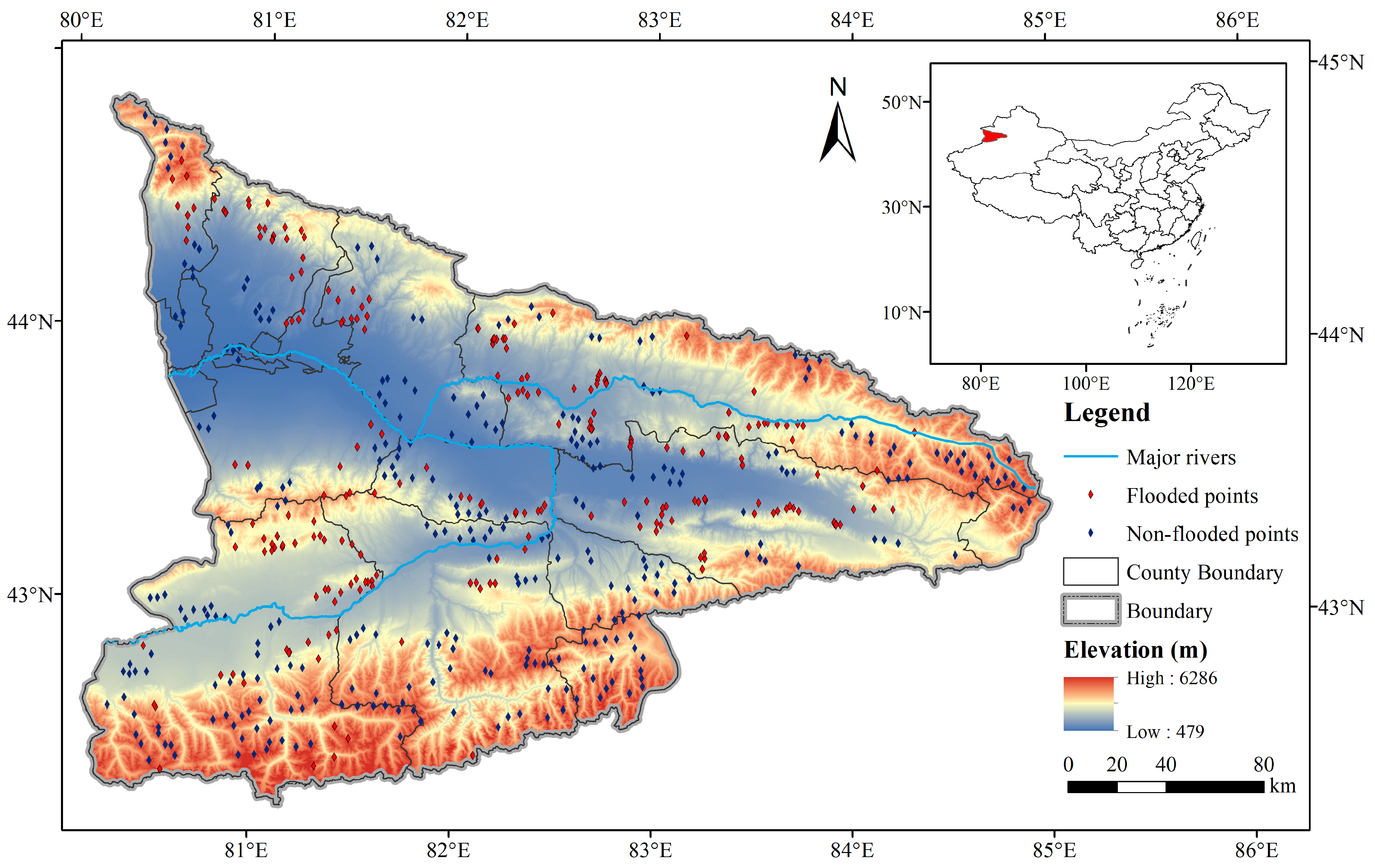
2.1. Study Area

The Ili River Basin in China (IRBC) is located in the northwest of China’s Xinjiang Uygur Autonomous Region. It is an important area for promoting the new development pattern for China’s Belt and Road Initiative. This transnational basin, shared with Kazakhstan, has experienced accelerated socio-economic development since 2000, driven by its unique geopolitical position and abundant natural resources. Characterized by diverse ecosystems spanning alpine glaciers to arid plains, the IRBC is relatively rich in natural resources such as water resources, flora and fauna, and human settlements. According to the Statistical Bulletin of National Economic and Social Development of Ili Kazakh Autonomous Prefecture in 2022, the population of the region was 2.85 million, accounting for 22.8% of the total population of Xinjiang, while generating CNY 280.1 billion in regional GDP [40].

The IRBC exhibits a drainage area of 57,000 km² with a perimeter of 1645 km. Topographically, the terrain descends east–westward with a mean elevation of 2006.3 m and an average slope gradient of 14.96°. The watershed exhibits a complex geological formation, with 12 active fault zones distributed from north to south, including the northern margin fault zone of the Yili Basin and the Kokobo River fault zone. The watershed is covered by a variety of vegetation, with grassland being the most widely distributed, covering an area of 33,306 square kilometers, followed by 9719 square kilometers of cropland. Due to the high percentage of grassland, the soil types within the mountains are diverse, which mainly include chestnut soil, chernozem, gray cinnamonic soil, and subalpine meadow soil.

Climatologically, the basin exhibits temperate continental conditions with pronounced precipitation gradients, with annual totals ranging from 497 mm to 222 mm. In the context of global warming, flash floods triggered by short-term heavy rainfall in the basin are on the rise from July to September each year.

Historical records document 317 flood events from 1980 to 2022, causing 156 fatalities and exceeding USD 2 billion in direct economic losses. Figure 1 shows the location of the study area and the distribution of validated flooded points within the IRBC.

2.2. Data

2.2.1. Flood Inventory Map

The flood inventory map synthesizes historical event records and spatiotemporal distribution patterns of flooding. In response to the flood disaster in the IRBC, the Ili State Emergency Response Department and the Water Resources and Meteorological Departments have established a detailed disaster dataset based on fieldwork. In this study, we used the flood observations provided by the Institute of Urumqi Desert Meteorology of the China Meteorological Administration (CMA), containing flood events in the IRBC from 1990 to 2022. These field-validated records, jointly maintained by local emergency management and hydrological agencies, include 309 historical flood sites distributed within the IRBC, which were used as flooded points in this study. To ensure spatial representativeness, these flooded points and 300 non-flooded points were systematically selected from various altitudes for the flood susceptibility and inundation analysis, as shown in Figure 1.

Satellite-based inundation mapping utilized the GEE platform to process Sentinel-1 Ground Range Detected (GRD) imagery from 2017 to 2023 and Landsat-5 TM and Landsat-7 ETM+ from 2000 to 2016. The Sentinel-1 SAR data in Interferometric Wide (IW) swath mode provides 10 m resolution observations with a 12-day revisit cycle, which is particularly effective for detecting sudden flood events [41]. Landsat’s multispectral capabilities with 30 m resolution complement this through long-term water body monitoring. This synergistic use of active and passive remote sensing enables a comprehensive analysis of the spatial and temporal distribution of inundation frequency. Both Sentinel-1 and Landsat data are available and can be processed on the GEE.

2.2.2. Flood Conditioning and Impact Factors

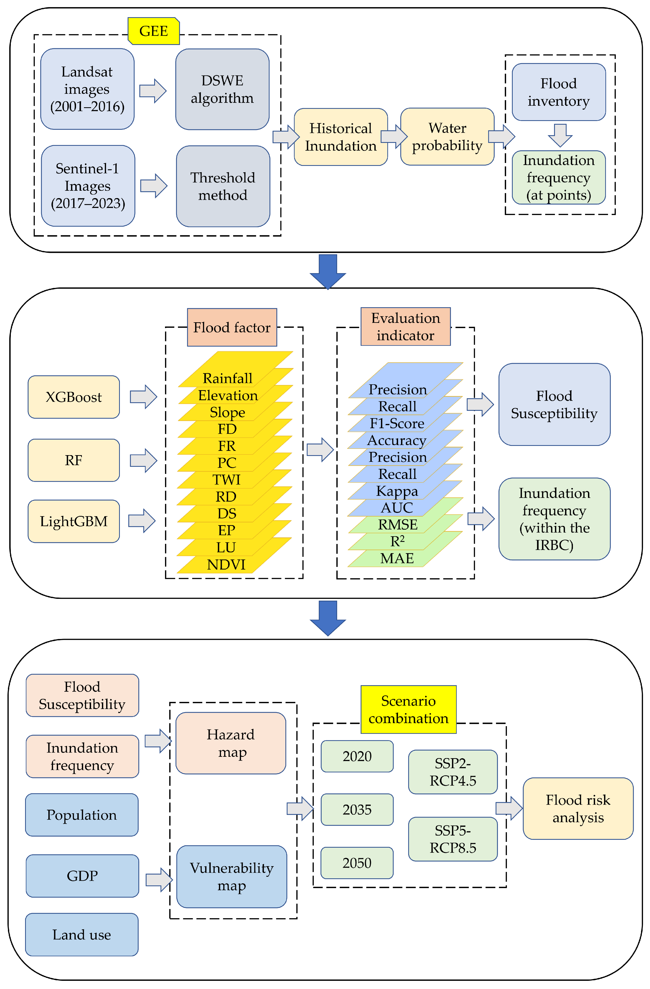
In this study, 13 flood conditioning factors were selected with reference to previous studies, including rainfall, elevation, slope, flow direction (FD), flow rate (FR), profile curvature (PC), river density (RD), distance to stream (DS), topographic wetness index (TWI), evapotranspiration (EP), curve number (CN), land use (LU), and normalized differential vegetation index (NDVI) [22,35,42]. These variables were sampled at both flooded points and non-flooded points to train the machine learning models.

Rainfall is the primary factor in inducing floods. Short-term heavy rainfall can easily trigger floods [42]. This study used the meteorological dataset of the Chinese region provided in the PANGAEA system, which contains daily minimum temperature, daily maximum temperature, and rainfall, spanning from 1961 to 2019 with a resolution of 1 km. In order to improve the accuracy of the dataset, measured rainfall data provided by the Institute of Urumqi Desert Meteorology of CMA were used for calibration. Daily rainfall datasets from 15 national meteorological stations and hourly rainfall data from 154 automatic stations were used as validation data. Based on the historical dataset, future rainfall data were obtained by calibrating NASA Earth Exchange Global Daily Downscaled Projections, CMIP6 (NEX-GDDP-CMIP6).

The major topographic factors, including slope, FD, FR, PC, and TWI, were generated from 12.5 m SRTM DEM using ArcGIS 10.7 hydrological tools [43]. These factors are indicative of the influence of topography on the accumulation of surface runoff and are responsible for the occurrence of flooding. CN is an indicative of the characteristics of the land and soil, which represent the surface characteristics related to floods. In a similar vein, land use, EP, and NDVI have been demonstrated to exert significant influence on surface runoff [44]. RD and DS reflect the distribution of streams, which describe the contribution of rivers to flood inundation.

RD and DW based on river data and NDVI were obtained from the Resource and Environment Science Data Platform (RESDC). EP was derived from the global terrestrial ecosystem evapotranspiration dataset MOD16A2, which was developed by NASA’s Earth Observing System Data and Information Center (EOSDIS). This dataset is available through GEE. The curve number (CN) was obtained from GCN250, which represents runoff for a combination of the European Space Agency global land cover datasets and geo-registered with the hydrologic soil group global data product [45]. The main datasets used are shown in

Table 1. The main datasets used in this study.

Datasets	Period	Resolution	Source
Sentinel-1 GRD	2017–2023	10 m	GEE
Landsat-5 TM and Landsat-7 ETM+	2001–2016	30 m	GEE
Annual maximum 1 h precipitation	1980–2023	1 km	PANGAEA; Institute of Urumqi Desert Meteorology of CMA
	2015–2100	0.1°	NEX-GDDP-CMIP6
Annual maximum 24 h precipitation	1980–2023	1 km	PANGAEA; Institute of Urumqi Desert Meteorology of CMA
	2015–2100	0.1°	NEX-GDDP-CMIP6
NDVI	1986–2022	30 m	RESDC [46]
Evaporation	2000–2022	500 m	MOD16A2
Curve number	2018	250 m	GCN250 dataset [45]
Land use	1985–2022	30 m	30 m annual land cover datasets [47]
	2020–2100	1 km	LULC projection datasets [48,49,50]
Population	2000–2020	100 m	WorldPop [51]
	2020–2100	1 km	Population projection datasets [52,53]
GDP	1995, 2000, 2005, 2010, 2015 and 2019	30 m	RESDC [54]
	2030–2100	0.25°	GDP projection datasets [52,55]

.

The vulnerability assessment incorporates historical and future projected socio-economic datasets for population, gross domestic product (GDP), and land use (LU). The historical population was estimated with WorldPop, and GDP was obtained from RESDC [51]. Historical land use data were based on the 30 m annual land cover datasets, which were formed by using 335,709 Landsat images on the Google Earth Engine [47]. Future projections aligned with shared socio-economic pathways (SSPs) were drawn from peer-reviewed spatializations, maintaining temporal consistency with CMIP6 climate scenarios [48,49,50,52,53,55].

2.3. Methodology

The following steps were used to assess flood risk: historical inundation extraction, prediction of flood susceptibility and inundation frequency, and flood risk estimation by combining hazard and vulnerability (Figure 2).

Initial historical inundation mapping synthesizes Landsat and Sentinel-1 imagery through GEE’s cloud processing capabilities, generating annual water occurrence frequencies from 2001 to 2023. Subsequently, three machine learning models (XGBoost, Random Forest, LightGBM) were trained using flood conditioning factors and observed inundation frequency at 609 sample points, enabling basin-wide projections of susceptibility and inundation probability. The final risk assessment combines these hazard components with vulnerability indicators, including population density, GDP, and land use, through a spatial overlay analysis. Temporal projections for 2020, 2035, and 2050 incorporate two SSP-RCP scenarios: the SSP2-RCP4.5 scenario (SSP2-4.5), representing moderate climate mitigation, and the SSP5-RCP8.5 scenario (SSP5-8.5), reflecting high-emission development pathways.

2.3.1. Multi-Temporal Satellite-Based Inundation Mapping

The inundation mapping protocol integrates multi-source satellite observations through a three-stage process. The open water extent was first extracted using the Dynamic Surface Water Area (DSWE) algorithm. DSWE was initially used by the USGS to classify land, open water, and partial water with several water-detecting tests [56]. We used the DSWE algorithm to calculate the number of times each pixel in the IRBC was classified and to calculate the probability of each classification. The DSWE dataset formed using this algorithm can be used on an a priori basis for further water extraction for Sentinel-1 SAR images [32,57].

Pre-processing is required before using the Sentinel-1 data. We accessed the Sentinel-1 GRD data using GEE and performed a coarse processing calibration using the platform toolbox, which contains operations such as orbital correction, thermal noise removal, radiometric calibration, and topographic correction. To remove the effect of anomalous backscatter values and scattering spots at the boundary, the images were subjected to additional boundary noise correction and scattering filtering using the Refined Lee filter [58,59]. The processed backscatter coefficients were converted to a decibel scale for the threshold analysis.

In order to obtain the water extent, DSWE-based thresholds were applied to the processed Sentinel-1 data. In this study, adaptive threshold determination followed the grid-based approach proposed by Chen et al. [57]. The algorithm divides the IRBC into 20 km grids and classifies the pixels in each grid into three categories, which are persistent land, persistent water, and partial water. The histogram type for each grid was determined based on the area proportion of each classification, employing the following formula:

$$H_c=\left\{\begin{array}{l}0,a{P}_w+b{P}_l\le P_t\\ 1,a{P}_w+b{P}_l>P_t,P_w>P_l\\ -1,a{P}_w+bP>P_t,P_w\le P_l\end{array}\right.$$

(1)

where $H_c$ is the histogram type parameter; $P_w$, $P_l$ and $P_t$ are the proportion of persistent water, persistent land, and partial water in each grid; and $a$ and $b$ are adjustable parameters. The histogram is considered to be bimodal when the percentage of partial water is significantly higher than the percentages of the other two categories; otherwise, it is single-peaked. Depending on the type of histogram, the threshold can be determined accordingly.

$$T=\left\{\begin{array}{l}{H}_v,H_c=0\\ \mu +3\sigma H_c,H_c\ne 0\end{array}\right.$$

(2)

where $H_v$ is the valley of the histogram; $\mu$ and $\sigma$ are the mean and variance, respectively; and $T$ is the threshold of the grid. Through stratified random sampling of nine grids covering different water proportions, we obtained the final threshold for the Sentinel-1 images as the average of the thresholds derived from these grids.

Typically, the extracted flood inundation should be the difference between the extracted water extent and the permanent water extent. In this study, the inundation input data for machine learning are limited to the historical flooded points. A review of data records indicates that the flooded points selected are situated in non-water areas for extended periods of time. The probability of persistent water at these points can be negligible. Accordingly, we calculated the probability of flood inundation by using the water probability at the historical flood sites.

To reduce the data processing time and ensure spatial consistency between the two remote sensing images, the pre-processed Sentinel-1 data were resampled to a resolution of 30 m before applying the threshold to delineate water bodies. By combining the extracted water extent from Landsat and Sentinel-1 data at a 30 m resolution, the water probability was calculated based on the number of times each pixel was detected as water in all images from both sources. The specific formula is as follows:

$$FP=(N_l{P}_l+N_s{P}_s)/(N_l+N_s)$$

(3)

where $N_l$ and $N_s$ are the number of occurrences of non-missing values from Landsat and Sentinel-1 data, respectively; $P_l$ and $P_s$ are the corresponding water probabilities; and FP represents the calculated historical water probability, which corresponds to the inundation frequency at the flooded points.

2.3.2. Machine Learning Methods

We employed XGBoost, RF, and LightGBM to evaluate the correlation between explanatory factors and target values [60,61,62]. In this study, flood susceptibility and inundation frequency were utilized as target values. Flooded points were labeled ‘1’ and non-flooded points were labeled ‘0’ for susceptibility mapping, while observed inundation frequencies served as continuous targets for the regression analysis.

XGBoost is recognized as one of the fastest decision tree algorithms currently available [63]. This algorithm constructs a strong learner by combining multiple weak learning models, utilizing Classification and Regression Tree (CART) as the base classifier. The input samples for each subsequent tree are informed by the residuals of previous trees [64]. The algorithm is particularly suited for handling sparse data due to its specialized split-finding strategy, and it demonstrates remarkable efficiency when processing large-scale datasets [39]. XGBoost is less prone to overfitting and more efficient than other gradient enhancement algorithms, primarily due to its parallelization of tree construction, cache block tree pruning, and other features [65].

RF is a versatile tool in the field of machine learning, offering capabilities in regression, classification, and data dimensionality reduction. It is a bagging ensemble learning algorithm consisting of multiple decision trees. The training samples and features of each decision tree are obtained through random sampling. The final prediction is obtained through a voting process on multiple decision trees. In the context of regression, the output of the Random Forest is the average of the outputs of all the decision trees. In the context of datasets with missing values, RF demonstrates enhanced robustness and adaptive ability while effectively mitigating the risk of overfitting [66]. The algorithm exhibits a rapid training speed and high accuracy in the context of datasets with uneven distribution and the absence of certain features [67].

LightGBM, developed by Microsoft, has emerged as one of the most effective machine learning algorithms based on gradient boosting on decision trees [68]. The algorithm employs a histogram-based approach to group features, thereby reducing the demand on memory resources. Unlike XGBoost, the generation of decision trees for the lightGBM algorithm is achieved through a leaf-wise growth strategy, as opposed to level-wise. The algorithm uses the GOSS method to split the entire dataset, sampling observations based on gradients. In comparison to the conventional boosting algorithm, this approach provides faster practice capability with higher precision [39].

The framework leverages binary classification outputs for susceptibility mapping and regression models for probabilistic inundation frequency estimation. Comparative performance analysis across algorithms informed the optimal model selection through rigorous statistical validation.

2.3.3. Model Performance Evaluation

In the case of binary classification problems, the evaluation of prediction is typically undertaken using indicators, including precision ($P$), recall ($R$), accuracy ($A$), F1-score ($F$), Kappa score ($K$), the Receiver Operating Characteristic curve (ROC), and the area under the curve (AUC) [42,66].

$$P={\displaystyle \frac{TP}{TP+FP}}$$

(4)

$$R={\displaystyle \frac{TP}{TP+FN}}$$

(5)

$$A={\displaystyle \frac{TP+TN}{TP+FP+TN+FN}}$$

(6)

$$F={\displaystyle \frac{2·P·R}{P+R}}$$

(7)

$$K={\displaystyle \frac{p_r-p_e}{1-p_e}}$$

(8)

where true positives ($TP$) denote instances where samples truly belonging to the positive class are correctly predicted as positive; false positives ($FP$) denote instances where samples from the negative class are erroneously predicted as positive; true negatives ($TN$) correspond to samples of the negative class being accurately identified as negative; false negatives ($FN$) indicate samples of the positive class that are incorrectly classified as negative; $p_r$ is the relative observed consistency among the evaluators; and $p_e$ is the assumed coincidence probability.

The ROC curve employs the False Positive Rate (FPR) as the horizontal axis and the True Positive Rate (TPR) as the vertical axis. The AUC calculated by the ROC constitutes a pivotal indicator for the evaluation of the overall performance of a model. Typically, a higher AUC value is indicative of a superior classification capability of the model [69].

To quantify the inundation frequency regression performance, this study calculated statistical indicators such as Mean Absolute Error (MAE), Root Mean Square Error (RMSE), and R2. These indicators describe the error between the predicted value and the true value. The lower the MAE and RMSE, the more accurate the model’s prediction; the higher the R2, the better the model predictions [70].

2.3.4. Flood Risk Assessment

In this study, flood risk was determined by combining hazard and vulnerability. Hazard mainly includes the probability and intensity of the causing factors. Inundation probability is an important factor that reflects the probability of flood occurrence. The greater the inundation probability, the greater the likelihood of flooding. The flood susceptibility determined by factors including rainfall, NDVI, and TWI, as described in Section 2.2.2, was used to assess the hazard from a different perspective. We obtained flood hazard maps by multiplying flood susceptibility by the inundation probability. Vulnerability measures the potential for socio-economic entities to incur losses as a result of flooding. The population and GDP are indicative of an area’s socio-economic status, while land use is a reflection of the extent to which the area is susceptible to flooding. These three socio-economic factors were selected as indicators of vulnerability.

The Analytical Hierarchy Process (AHP) is a subjective assignment evaluation method. This study used the AHP to determine the weights of the indicators to determine the flood vulnerability. This method involves the decomposition of the complex problem into a hierarchical structure consisting of objectives, criteria, and alternatives. A judgment matrix is then constructed based on the model in order to calculate the weights. Following consistency checking and weight combination, the final result is obtained [71]. Based on the subjective determination of the weights of the criteria, the weights of the vulnerability factors were determined by the AHP, as shown in Formula (10).

In light of the aforementioned analysis, the risk expression is as follows:

$$Hazard=Susceptibility\times Frequency$$

(9)

$$Vulnerability=0.35\times Population+0.41\times GDP+0.24\times LandUse$$

(10)

$$Risk=Hazard\times Vulnerability$$

(11)

In order to reflect the role of indicators in determining the value at risk, we employed the multiple linear regression to calculate the relative contribution of each indicator to the risk [72].

$$r_n={\displaystyle \sum _{i=1}^5{a}_{n,i}{x}_{n,i}+b_n}$$

(12)

$$C_n={\displaystyle \frac{a_{n,i}}{{\displaystyle \sum _{i=1}^5{a}_{n,i}}}}\times 100\%$$

(13)

where $r_n$ is the normalized risk value of the scenario ‘n’; $x_{n,i}$ represents the normalized risk indicator; $a_{n,i}$ represents the regression coefficients and $b_n$ is the intercept; $C_n$ is the percentage contribution of each indicator to the risk.

3. Results

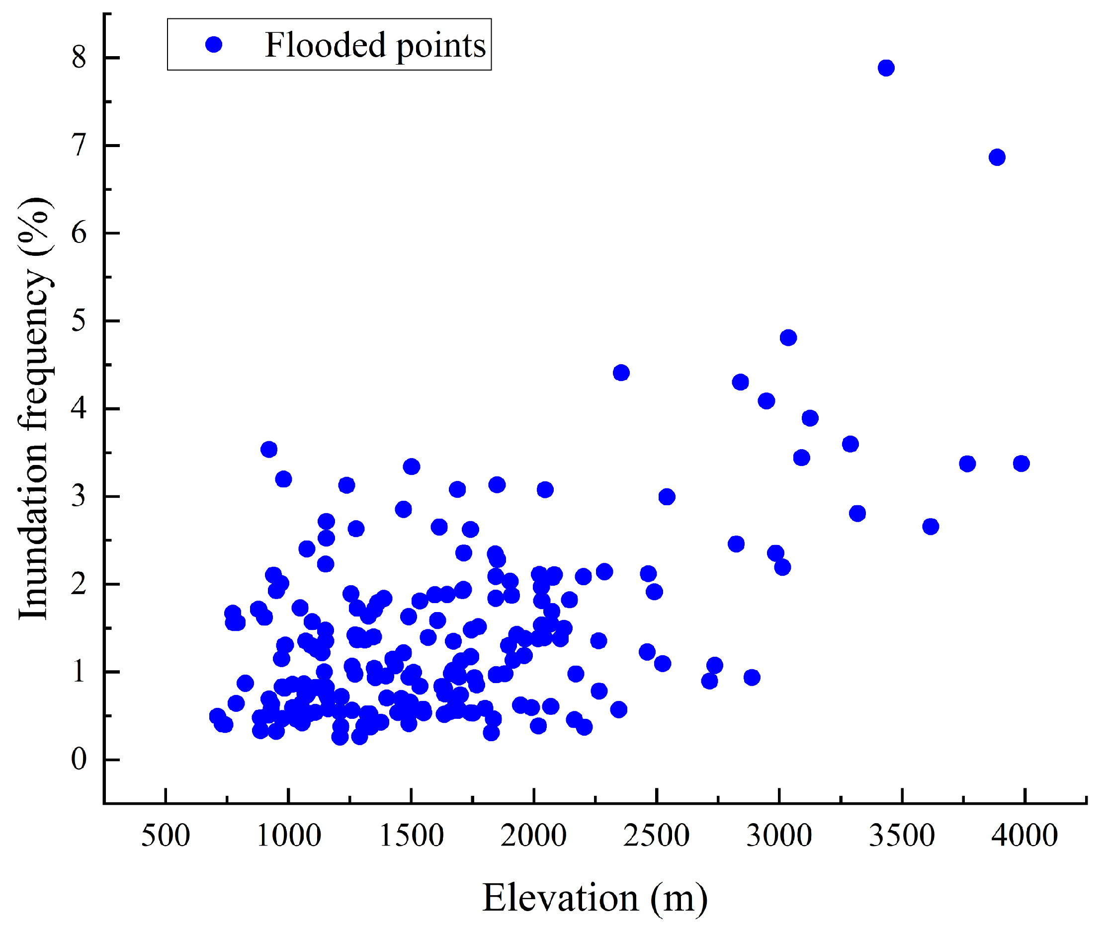
3.1. Analysis of Historical Inundation Patterns

In order to ensure consistency between the historical event inventory and the satellite observations, a comparison was made between the dates of the historical flood records and remote sensing imagery. We found that 20 out of 25 floods occurring between 2017 and 2023 had dates that corresponded to Sentinel-1 images, and 146 of 220 floods between 2001 and 2016 had dates that corresponded to Landsat images. Twenty-three floods affecting over 1000 people went unrecorded by satellite imagery. Due to the wide coverage of Landsat and Sentinel-1 imagery, more than 80% of major regional floods affecting more than 1000 people were effectively captured.

The threshold for Sentinel-1 data was calculated by sampling nine areas containing flooded points according to Formulas (1) and (2). The sampling areas were selected from regions with documented historical instances of significant floods, including flood-prone areas in Xinyuan, Nilka, and Tekesi. These areas are suitable for testing flood inundation extraction due to the environmental impacts that have resulted in repeated floods. Based on the feature comparison calibration, we obtained a threshold of −22.68 dB for the VH band. In order to verify the reliability of the threshold extraction, five typical flood events from 2001 to 2023 were subjected to visual comparison. Validation using Sentinel-2 true-color composite images demonstrated an overall accuracy of 92.3% at the flooded points, indicating a superior extraction result. By using this threshold, we extracted the water extent from Sentinel-1 imagery. Integration with Landsat-derived DSWE produced the water probability map for the period of 2001 to 2023, as shown in Figure 3.

Spatial analysis revealed 6647 km² of stable non-flooded areas (water probability < 1%) concentrated in eastern plains, contrasting with 2436 km² of high-frequency flood zones (water probability > 50%) along major rivers. While permanent snow cover in alpine regions (>3000 m) caused 12.7% false positives in water detection, this systematic error does not affect flood risk assessment since 99.3% of validated flooded points occur below 2500 m elevation.

The inundation frequency statistics for the flooded points are shown in Figure 4. The results show that the inundation frequency at most of the flooded points is less than 5%, concentrated in areas lower than 3000 m. It shows a tendency for the inundation frequency to increase with higher elevation.

3.2. Comparative Performance Evaluation of Machine Learning

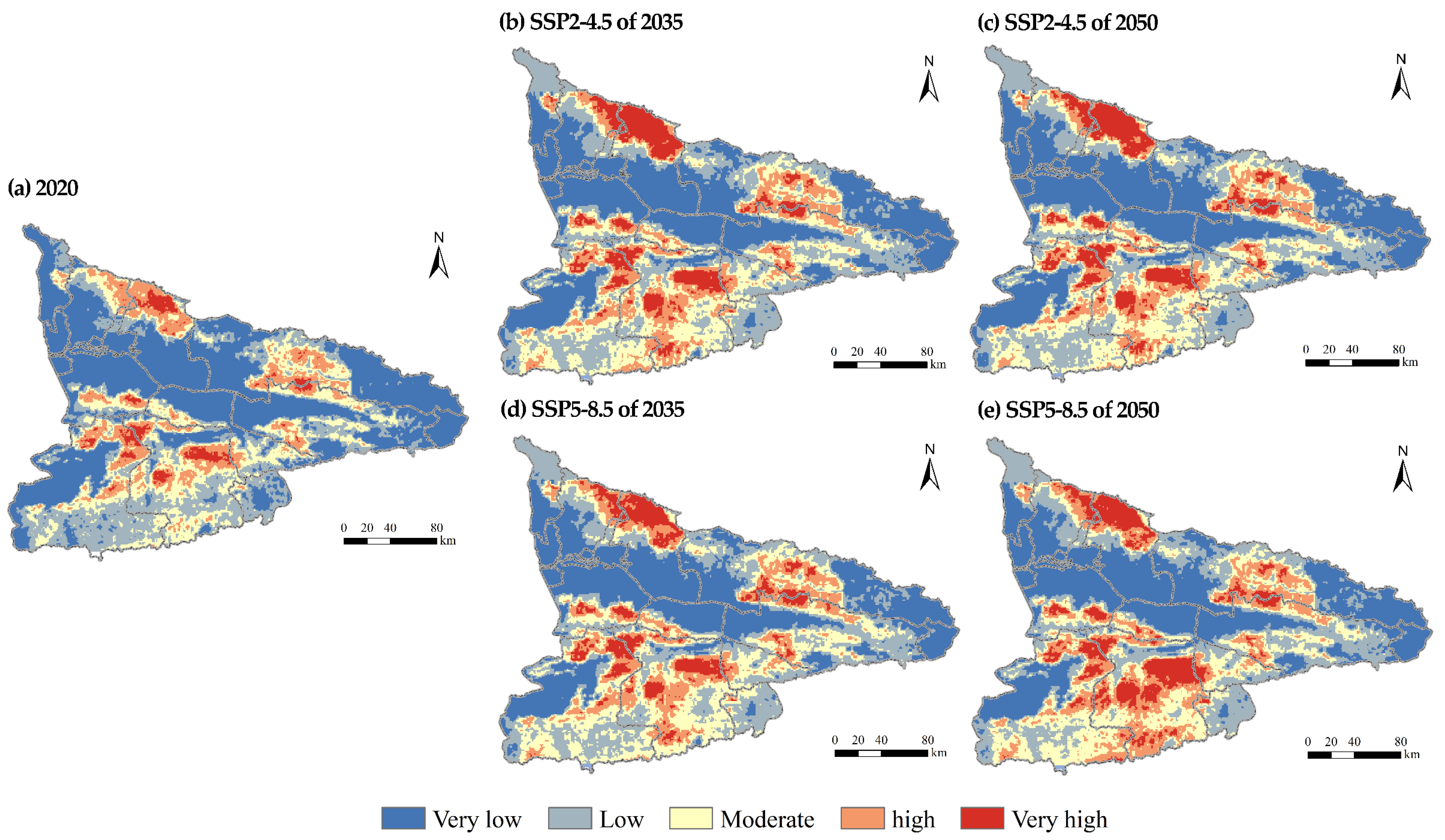
The classification performance evaluation of the three machine learning models is measured by five indicators, as shown in

Table 2. Evaluation results of the LightGBM, RF, and XGBoost model classifications.

Model	Precision (%)	Recall (%)	F1-Score (%)	Accuracy (%)	Kappa
LightGBM	89.19	86.84	88.00	88.08	0.76
RF	89.47	89.47	89.47	89.40	0.79
XGBoost	93.33	92.11	92.72	92.72	0.85

. Compared to LightGBM and RF, XGBoost demonstrates superior performance in terms of precision, recall, accuracy, and F1-score, with all indicators exceeding 90%. The Kappa score of XGBoost is 0.85, which proves the model has good performance [42]. ROC curves and AUC values were also used to analyze the performance of the model classifications (Figure 5). The AUC values calculated by LightGBM, RF, and XGBoost are approximately equal to 0.96, with XGBoost demonstrating the highest AUC value.

The performance of the model regression function was assessed by MAE, R², and RMSE, as shown in

Table 3. Evaluation results of the LightGBM, RF, and XGBoost model regression.

Model	RMSE	R2	MAE
LightGBM	0.04	0.79	0.03
RF	0.03	0.82	0.02
XGBoost	0.01	0.96	0.01

. The RMSE and MAE for XGBoost are both approximately 0.01, while the RMSE and MAE for RF are 0.04 and 0.03, respectively, and the RMSE and MAE of LightGBM are 0.03 and 0.02, respectively. The R² for XGBoost is 0.96, which is significantly higher than the values of 0.82 for RF and 0.79 for LightGBM. The analysis of the model classification and regression indicates that XGBoost exhibits superior performance in comparison to LightGBM and RF. Given these statistically significant advantages, XGBoost was selected for the spatiotemporal projection of flood hazards under SSP-RCP scenarios.

3.3. Flood Risk

3.3.1. Flood Hazard

High-resolution mapping can provide a wealth of information for flood risk management. However, due to the resolution limitations of datasets such as population, GDP, and land use, especially future projection datasets, calculations on higher-resolution grids may lead to inaccurate results. To ensure the correct prediction of the flood risk distribution, this study integrated datasets with a 1 km resolution for flood hazard, vulnerability, and risk mapping.

The spatial distributions of flood susceptibility and inundation frequency were both calculated based on XGBoost. By applying the natural break method, we obtained hazard maps, which classified the IRBC into five classes: very low, low, moderate, high, and very high (Figure 6) [73].

The results showed that in 2020, the very high class covers 2.6% of the IRBC and the high class covers 15.1% of the area (

Table 4. Area proportion and range of each flood hazard class in the SSP2-4.5 and SSP5-8.5 scenarios from 2020 to 2050.

Area (%)	2020	2035		2050		Range
		SSP2-4.5	SSP5-8.5	SSP2-4.5	SSP5-8.5
Very low	33.6	35.3	33.8	35.2	33.9	0–0.03
Low	22.9	25.1	25.1	25.8	23.8	0.03–0.06
Moderate	25.9	18.6	20.8	19.0	18.6	0.06–0.09
High	15.1	13.3	13.2	12.1	15.1	0.09–0.11
Very high	2.6	7.7	7.0	7.9	8.6	0.11–0.16

). These areas dominate the central and northern parts, especially around the Tekes and Yili rivers. The distributions of low-hazard (33.6%) and very-low-hazard (22.9%) areas are concentrated in the midwestern and northeastern regions, aligning with lower elevations of less than 1800 m.

In SSP2-4.5, compared to 2020, there is a significant increase in the very-high-hazard areas in 2035 and 2050 by 4.9% and 5.3%, respectively. The increase would be particularly pronounced in the northern and southern alpine regions. In SSP5-8.5, the increase in very-high-hazard areas would be 4.4% in 2035 and 6.0% in 2050. The range of high- and very-high-hazard areas under this scenario is similar to that of SSP2-4.5, except in the southern mountainous areas.

Despite the greater increase in very-high-hazard areas in SSP2-4.5 than in SSP5-8.5 in 2035, the intensity of hazard increase in SSP2-4.5 would significantly reduce from 2035 to 2050, while the high- and very-high-hazard areas in SSP5-8.5 would still significantly increase in the southern and central parts of the IRBC. In SSP5-8.5 in 2050, the percentage of high- and very-high-hazard areas would reach 23.7%. Overall, the increase in hazard was stronger in the short term in SSP2-4.5 and greater in the long term in SSP5-8.5.

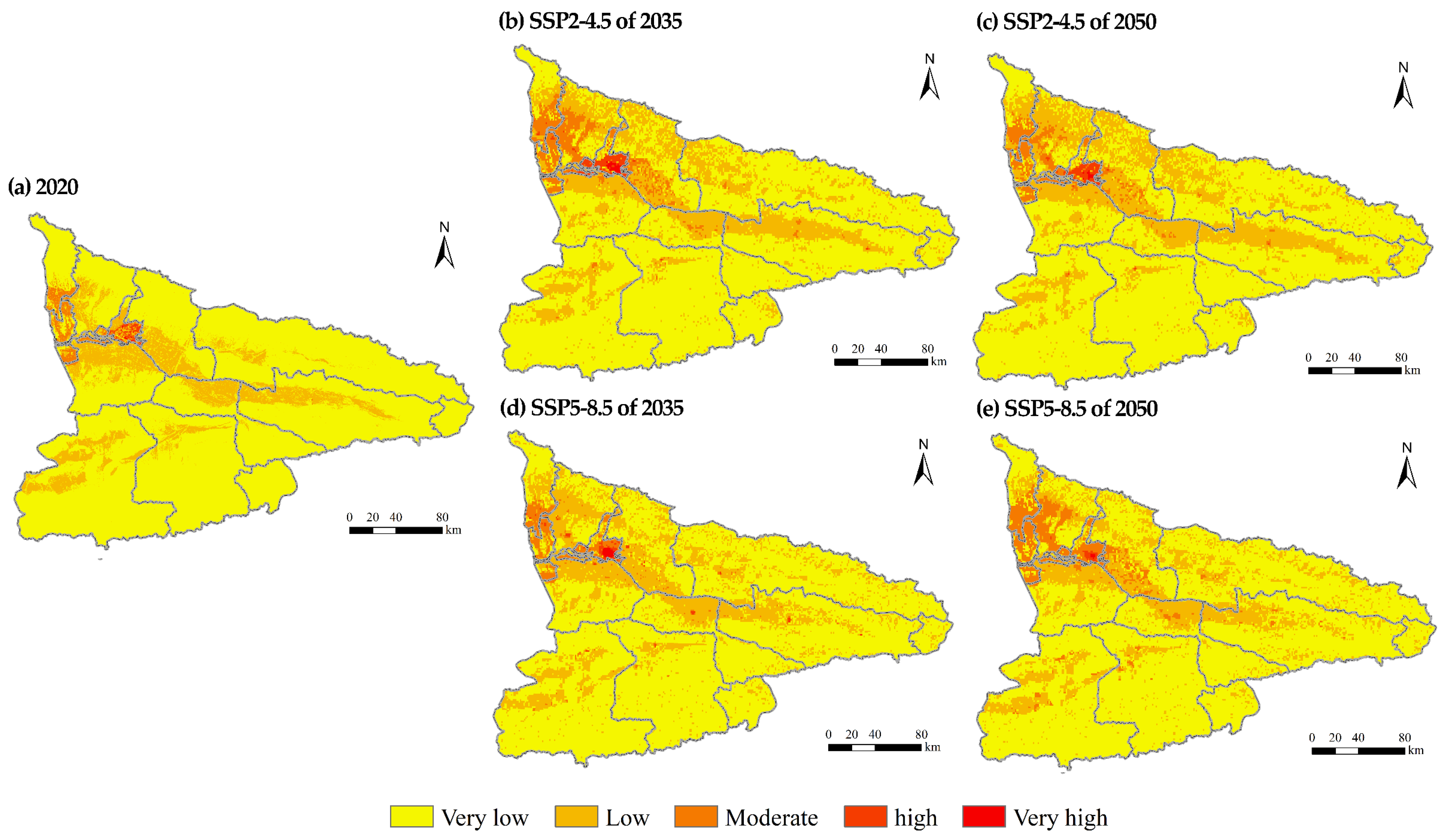
3.3.2. Flood Vulnerability

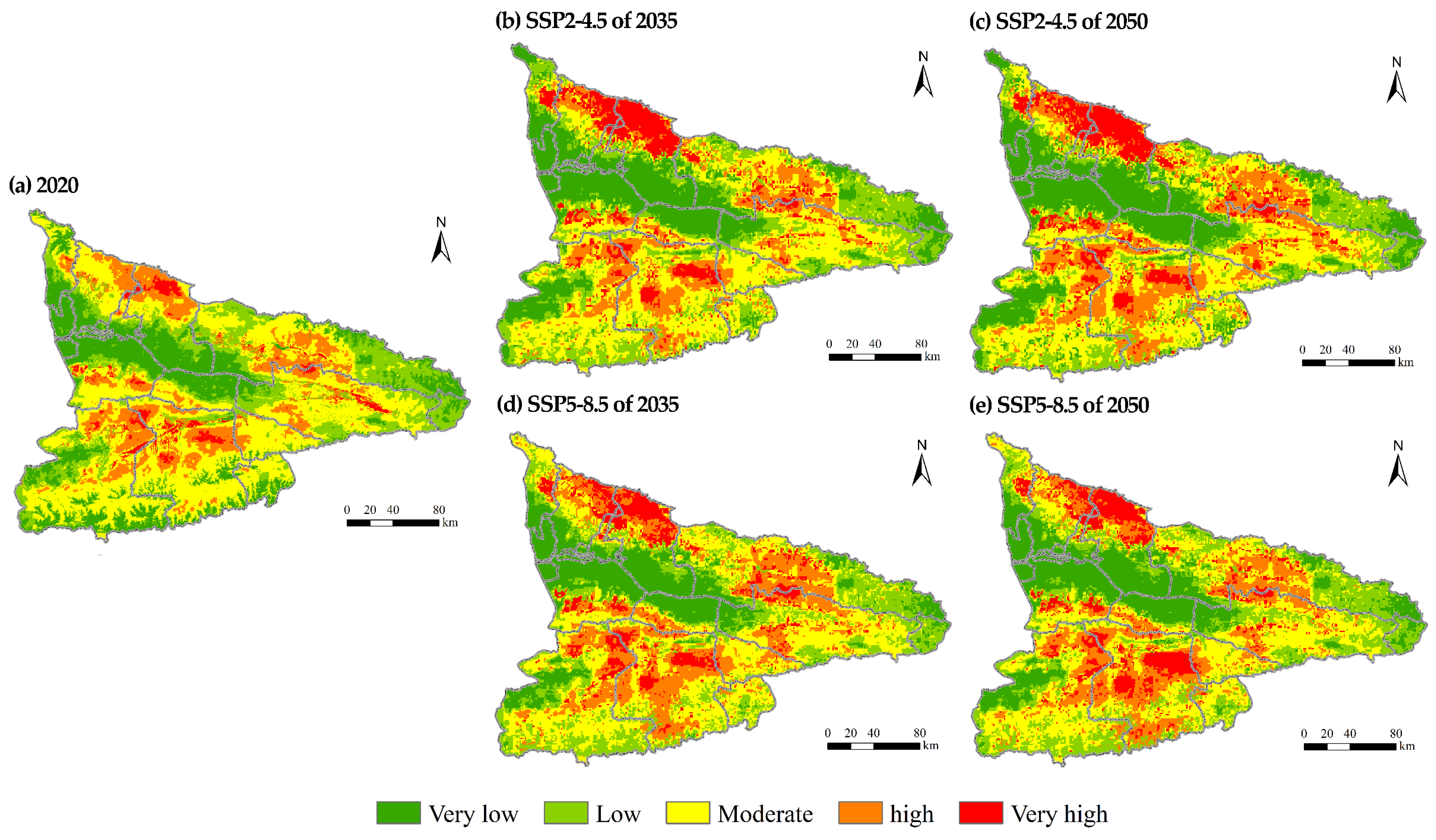
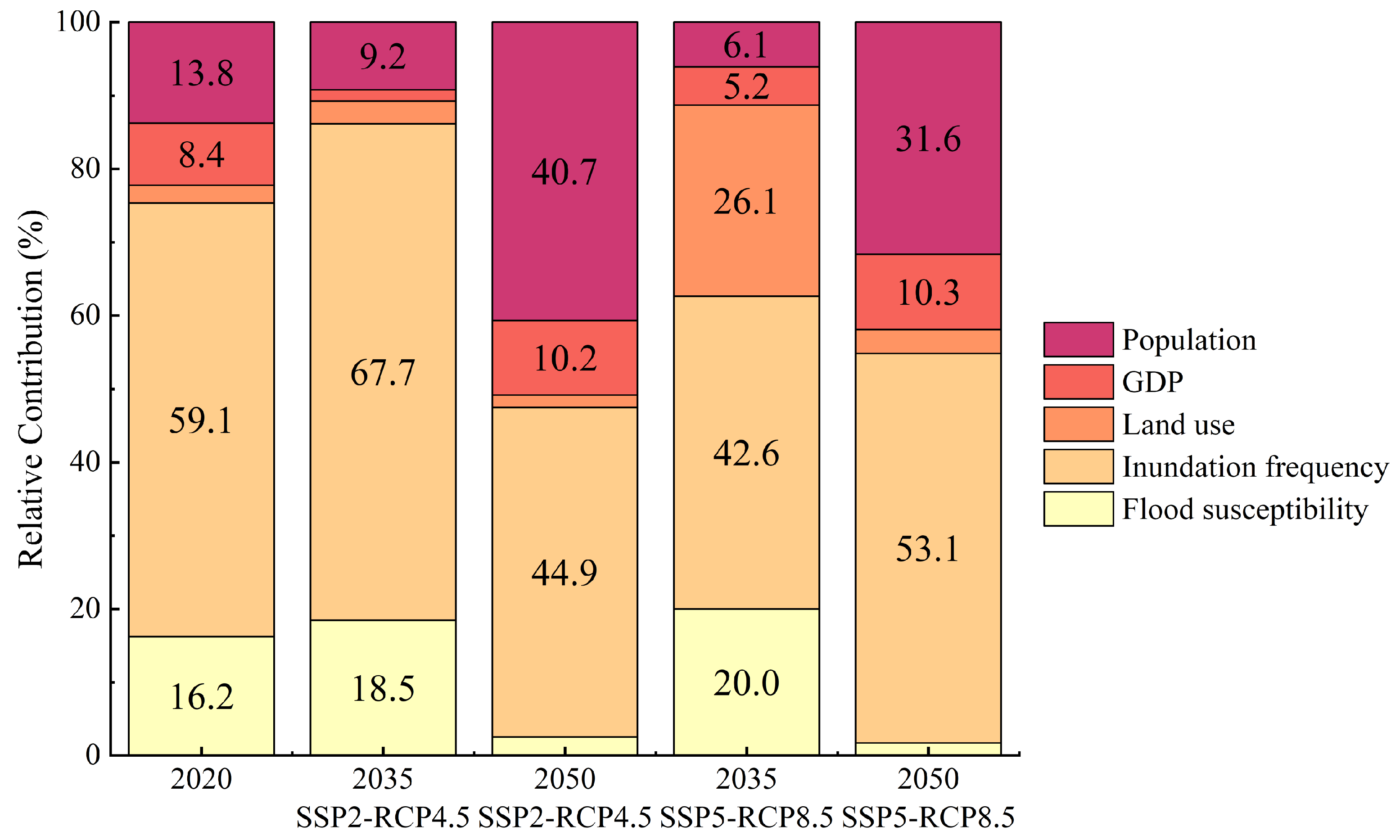
Flood vulnerability maps were obtained by combining population, GDP, and land use. Figure 7 shows the changes in population, GDP, and land use from 2020 to 2050 in the two scenarios. The population in the IRBC would grow from 2020 to 2035, followed by a decline between 2035 and 2050, in both scenarios. The population of Yining City, the city with the highest population density, would decline from 1.02 million to 0.87 million between 2020 and 2035, and further to 0.85 million by 2050 (0.82 million in the SSP5). This urban core depopulation drives 24–75% population growth in peripheral counties from 2020 to 2035, reflecting rural–urban demographic redistribution.

Economic projections indicate sustained GDP growth across scenarios, expanding from CNY 233.8 billion in 2020 to 382.5 billion in 2035 (408.1 billion in the SSP5) and to 621.9 billion in 2050 (676.2 billion in the SSP5). As total GDP grows, the range of GDP in different regions will continue to expand (Figure 8b).

The area of cropland within the Ili River is projected to increase in response to population growth and economic development. The area of cropland expands from 9054 km² under the SSP2 scenario to 14,177 km² in 2035 and 14,939 km² in 2050. In contrast, in the SSP5 scenario, the expansion of cropland area is projected to occur at a more gradual pace, increasing from 12,091 km² in 2035 to 13,142 km² in 2050. These changes are mainly concentrated in the north and east, especially in Huocheng and Yining counties.

Flood vulnerability changes in the IRBC are shown in Figure 8. Areas of high and very high class in 2020 cover 0.4% of the study area, mainly concentrated in Yining and Horgos (

Table 5. Area proportion and range of each flood vulnerability class in the SSP2-4.5 and SSP5-8.5 scenarios from 2020 to 2050.

Area (%)	2020	2035		2050		Range
		SSP2-4.5	SSP5-8.5	SSP2-4.5	SSP5-8.5
Very low	83.75	71.07	74.29	70.60	73.70	0–0.15
Low	14.18	23.03	22.52	25.16	20.32	0.15–0.25
Moderate	1.65	4.83	2.72	3.50	5.82	0.25–0.29
High	0.38	0.91	0.33	0.69	0.14	0.29–0.41
Very high	0.04	0.15	0.13	0.05	0.02	0.41–0.93

). In SSP2-4.5, the high- and very-high-class areas increase to 1.1% in 2035 and decrease to 0.7% in 2050. In SSP5-8.5, the high- and very-high-class areas cover 0.5% in 2035 and decline to 0.2% of the IRBC in 2050. Throughout these changes, Yining City would be at the center of the high-vulnerability areas. In both scenarios, the IRBC is projected to show a tendency of vulnerability to increase and then decrease. This suggests that from 2020 to 2035, increasing GDP in the center region will continue to increase areas of high vulnerability. Conversely, from 2035 to 2050, the redistribution of population and the dispersion of cropland area will result in a decline in the concentration of high vulnerability. In SSP5-8.5, the decline in vulnerability is more pronounced, implying a more decentralized distribution of population, cropland, and GDP in the future. Due to the population migration and changes in the cropland area, part of the northern IRBC will increase from a very low class to a low class in both scenarios from 2020 to 2050. In the northeastern part of the IRBC, in Huocheng and Horgos, the moderate vulnerability area is projected to expand and will be more pronounced in SSP2-4.5 than in SSP5-8.5.

3.3.3. Flood Risk

The flood risk maps were obtained by combining flood hazard and vulnerability (Figure 9). The very high class covered 3.5% of the IRBC, while the high-class area covered 14.4% (

Table 6. Area proportion and range of each flood hazard class in the SSP2-4.5 and SSP5-8.5 scenarios from 2020 to 2050.

Area (%)	2020	2035		2050		Range
		SSP2-4.5	SSP5-8.5	SSP2-4.5	SSP5-8.5
Very low	24.6	23.7	25.5	19.0	20.7	0–0.005
Low	18.0	21.9	17.8	21.5	23.0	0.005–0.009
Moderate	39.4	30.0	27.5	30.5	28.6	0.009–0.018
High	14.4	14.9	18.9	20.1	20.2	0.018–0.024
Very high	3.5	9.4	10.3	8.9	9.5	0.024–0.046

). In SSP2-4.5, the total area of the high- and very-high-class areas showed a rapid growth trend, increasing to 12,775 km² (24.3%) in 2035 and 15,302 km² in 2050 (29.1%). The expansion of the high class is concentrated in the southwestern plains, which used to be dominated by the moderate class. The increase in very-high-class areas is concentrated in the northwestern mountains. In SSP5-8.5, the sum of the high- and very-high-class areas increases more rapidly, reaching 28.9% in 2035 and 29.7% in 2050. In comparison with SSP2-4.5, the high- and very-high-class areas exhibited a reduced increase in the southwestern and northwestern high areas, while novel increases were observed in the southern mountains of the IRBC.

Driver analysis through multivariable linear regression identified shifting dominance patterns in flood risk (Figure 10). In both scenarios, the contribution of inundation frequency to flood risk is the most significant. Between 2020 and 2035, the relative contribution of inundation frequency changes from 59.1% in 2020 to 67.7% in SSP2-4.5 and 42.6% in SSP5-8.5 in 2035. By 2050, the contribution of the vulnerability indicators will increase. This tendency is strongest in SSP2-4.5, where the contribution of the population reaches 40.7%, and the total contribution of three vulnerability indicators reaches 52.6%. This represents a critical regime shift where anthropogenic factors surpass hydroclimatic drivers in governing long-term flood risks.

4. Discussion

4.1. Flood Risk Assessment Integrating Remote Sensing and Machine Learning

Flood risk is influenced by a wide range of natural and socio-economic factors. Based on the analysis of multiple features, researchers have been working on a more comprehensive interpretation of flood risk. Flood characteristics such as flood depth, flood velocity, and flood susceptibility are frequently employed to delineate flood hazard [39,74,75]. Zheng et al. quantified flood resilience as a complementary concept to flood risk [12]. Aerts et al. integrated social behavior and behavioral adaptation dynamics into flood risk assessment for a more accurate characterization of risk [76]. In order to compensate for the description of the temporal characteristics of floods, this study combines the inundation frequency obtained from remote sensing imagery with flood susceptibility. The composite description of the occurrence and frequency of flooding is conducive to the enhanced interpretation of flood risk.

The utilization of satellite-based inundation mapping in near-real time has been demonstrated to be an effective tool for the assessment of flood risk [77]. SAR-based Sentinel-1 provides remote sensing imagery with a high degree of clarity in distinguishing water bodies from land. The combination of Sentinel-1 data with the DEM allows for rapid mapping of the flood extent and depth [78]. In order to include more flood events over a wider time period, we utilized Landsat as a support. As a long-term Earth observation programme, Landsat satellites have been providing remote sensing images of progressively higher quality since 1972 [79]. These data facilitate widespread access to flood information [80]. In this study, Landsat was instrumental in establishing the threshold calculations, while also bridging the absence of Sentinel-1 imaging until 2017. This combination of multi-source imagery has been shown to enhance the efficiency of flood monitoring [32,78].

Machine learning methods facilitate the establishment of the mechanism by which natural factors are associated with floods, on the basis of obtaining flood characteristics [81]. In this study, three models were used in the prediction of flood susceptibility and inundation frequency. XGBoost outperformed the other two machine learning models in both classification and regression functions. In a similar vein, XGBoost has been shown to demonstrate better performance than RF and LightGBM in a number of tasks [82,83]. Our study utilized indicators to evaluate the performance of each model in predicting floods and non-floods. The higher precision and recall of XGBoost prove its superiority in predicting positive and negative class instances. In fact, XGBoost integrates the prediction results of all basic learners, thus elevating its recognition rate and generalization ability [42]. The algorithm is not affected by multicollinearity, making the selection of indicators have less impact on the overfitting of the model. This property allows XGBoost to perform better when using multiple terrain factors with correlated characteristics [84]. However, it should be noted that XGBoost does not demonstrate superior performance in all instances. In the study conducted by Guo et al., the prediction accuracy of XGBoost was found to be inferior to that of LightGBM when utilizing these algorithms to predict groundwater potential [62]. The acquisition of accurate climate data will enable LightGBM to exhibit higher accuracy. Consequently, it is recommended to utilize multiple models for comparison and selection of the most suitable model for the specific scenarios in which they are employed.

4.2. Flood Risk Changes in SSP-RCP Scenarios

Our results demonstrate that future flood risks in the Ili River Basin are projected to increase under both SSP-RCP scenarios. This finding aligns with previous studies which highlight the increasing impact of climate change on global extreme hydrological events. According to Zittis et al., the rapid growth of greenhouse gas emissions in the Eastern Mediterranean and Middle East region has led to an increase in heat waves and flash flooding events [85]. Tang et al. observed that both climate change and urbanization have led to an increase in urban flooding and that the contribution of climate change is more substantial in China [86]. Davenport et al. predicted that precipitation extremes driven by climate change in the United States will increase flood damages over the next 30 years [87]. The findings of this study indicate that the risk of flooding continues to increase, even in the IRBC, which is situated in the arid regions of Xinjiang, China. Indeed, the sudden turn from drought to flood is becoming increasingly prominent. Wang et al. observed that this trend has become increasingly prevalent in northern China, a phenomenon attributable to the heightened frequency of floods and the increasing variability of precipitation [88]. A similar phenomenon has been observed in California, a state that has been particularly damaged by severe drought. According to Huang, climate change has already led to a doubling of the likelihood of flooding events in the arid regions of California [89].

Our scenario comparison analysis shows that in SSP2-4.5, flooding events are a major factor in driving risk exacerbation due to short-term flooding events, while in SSP5-8.5, risk impacts are more pronounced due to the assumed increase in greenhouse gas emissions and more intensive socio-economic development. In the long term, the greater impact of socio-economic development will result in a higher risk under SSP5-8.5 than under SSP2-4.5, as is well documented in global research. Wang et al. indicated that the areas with high flood susceptibility are more overlapped with the populated urban center in SSP5-8.5 compared to SSP2-4.5 [90]. According to Adnan et al., the construction of polders led to significant changes in land use, which in turn increased the risk of flooding [91]. In the SSP5-8.5 scenario, the increase in cropland area is identified as a significant causal factor contributing to elevated risk levels of the IRBC.

Compared to previous studies, the incorporation of SSP-RCP frameworks in this study allowed for a more comprehensive analysis of flood risk by accounting for both climatic and non-climatic factors. This holistic approach emphasizes the importance of integrating socio-economic variables and flood inundation into flood risk assessments, particularly in regions undergoing rapid development and urbanization.

4.3. Indications for Flood Risk Management

One of the most significant contributions of this research is its potential application in flood risk management for data-scarce regions. The proposed methodology offers a transferable framework that can be adapted to other river basins facing similar data limitations. The use of remote sensing to reconstruct historical flood inundation patterns proved effective in addressing the challenge of limited ground-based observational data [32]. Combined with remote sensing information extraction, machine learning has been demonstrated to achieve high levels of accuracy in prediction, especially in areas where detailed hydraulic and hydrological data are not available [92]. Through the analysis of indicator contributions, we were able to identify the key drivers of flood risk, such as precipitation, inundation frequency, land use changes, and anthropological factors. This framework facilitates the effective prediction of flood impacts in areas with limited data availability by leveraging the utilization of publicly accessible datasets.

The management of flood risk necessitates the implementation of a variety of adaptation measures [93]. This study can inform the development of targeted adaptation measures, such as improved land use planning, enhanced early warning systems, and infrastructure investments aimed at mitigating flood impacts. According to Boulange et al., dams have been shown to have a substantial impact on reducing population exposure to flooding [94]. Building codes and nature-based measures are also relevant as a complement to flood-resistant buildings. This study analyzes each indicator of risk composition and its contribution separately. This can assist decision makers in the selection of management measures for particular control targets. According to Rentschler et al., low-income people in regions at high risk of flooding should be given higher priority [95]. Individuals with higher incomes frequently exhibit a greater propensity to opt for residence in areas that are less susceptible to flooding. For instance, in the case of IRBC, by the year 2050, when the population’s contribution to flood risk is substantial, control measures ought to prioritize the evacuation of low-income populations residing in flood-prone areas. In the year 2035, the relative contribution of land use will be substantial. Initiatives such as flood storage basins and the preservation and regeneration of forests in flood-prone areas should be accorded a high priority [96].

This methodology not only provides a robust framework for understanding past flood events but also enables the projection of future risks under different climate and socio-economic scenarios. By considering different conditions, policymakers can better prepare for a range of potential futures, thereby enhancing the resilience of vulnerable communities.

4.4. Limitations of the Study

Despite its contributions, this study has several limitations. First, the accuracy of the flood inundation maps derived from remote sensing data is influenced by the resolution and quality of the satellite images used. Some small-scale or short-duration flood events may not be accurately captured. In areas with complex terrain or dense vegetation cover, the uncertainty of flooding extraction still exists, while the threshold cannot be adjusted for each image. In addition, the machine learning models used in this study rely on historical data for classification and prediction. Model performance is contingent on the representativeness of the training data. In regions where historical flood events are poorly documented, the reliability of these models may be compromised. This study considers only two SSP-RCP scenarios and flood changes through four risk indicators. While the SSP-RCP scenarios provide a valuable framework for assessing future risks, they are inherently subject to uncertainties related to socio-economic trajectories and climate models. These uncertainties should be acknowledged when interpreting the results and formulating policy recommendations.

Building on the findings of this study, our future research should aim to address the identified limitations and further refine the proposed methodology. For instance, efforts could be directed toward integrating higher-resolution remote sensing data and incorporating additional variables, such as flood depth and flood resilience, to provide a more comprehensive explanation of flood risk. There is also a need for more localized studies that consider adaptive capacities. By combining quantitative modeling with qualitative methods, researchers can develop solutions for flood risk management that are more responsive to future changes.

In general, there is a necessity for an enhanced database to facilitate reliable risk assessment, particularly in the IRBC. Long-term monitoring and data collection efforts should be prioritized in data-scarce regions to enhance the availability and quality of hydrological and socio-economic datasets. These efforts will not only improve the reliability of future assessments but also contribute to a deeper understanding of the complex interactions between climate change, socio-economic development, and flood risks.

5. Conclusions

This study establishes an integrated flood risk assessment framework combining remote sensing and machine learning. The combination of Sentinel-1 SAR imagery and Landsat multi-temporal observations from 2001 to 2023 enabled the calculation of historical inundation frequency. Based on the historical inundation frequency and flood conditioning factors at flooded points, we used XGBoost, lightGBM, and RF models to predict flood susceptibility and inundation frequency in the IRBC. The methodology was applied to assess risks under two SSP-RCP scenarios for 2020, 2035, and 2050, integrating vulnerability indicators such as population, GDP, and land use patterns.

The flood risk results revealed distinct spatial–temporal risk patterns, with high- and very-high-risk areas expanding from 17.9% in 2020 to 29.1% in SSP2-4.5 and 29.7% in SSP5-8.5 by 2050. The contribution analysis reveals a temporal shift in risk drivers: inundation frequency dominates in the short-term risk evolution, with contribution changes from 59.1% to 67.7% between 2020 and 2035. Vulnerability factors gain prominence in the long-term risks, particularly population, which contributes 40.7% in SSP2-4.5. Spatially, northwestern mountainous regions face intensifying hazards from altered precipitation regimes, whereas urban centers like Yining exhibit high risks through concentrated vulnerability.

These findings carry significant practical implications for climate adaptation: machine learning-derived hazard maps enable the spatial optimization of early warning systems, while scenario-based vulnerability analysis establishes quantitative foundations for differentiated policy formulation. This framework ultimately demonstrates the practical value of open geospatial data and intelligent algorithms in enhancing regional climate resilience.

References

1. CRED; UNDRR. The Human Cost of Disasters: An Overview of the Last 20 Years (2000–2019). Available online: https://www.undrr.org/publication/human-cost-disasters-overview-last-20-years-2000-2019 (accessed on 17 February 2025).
2. IPCC. Climate Change 2021—The Physical Science Basis: Working Group I Contribution to the Sixth Assessment Report of the Intergovernmental Panel on Climate Change; Cambridge University Press: Cambridge, UK, 2023. [Google Scholar]
3. Clement, V.; Rigaud, K.K.; de Sherbinin, A.; Jones, B.; Adamo, S.; Schewe, J.; Sadiq, N. Groundswell Part 2: Acting on Internal Climate Migration. Available online: https://hdl.handle.net/10986/36248 (accessed on 17 February 2025).
4. UNDRR. GAR Special Report 2023: Mapping Resilience for the Sustainable Development Goals. Available online: https://www.undrr.org/gar/gar2023-special-report (accessed on 17 February 2025).
5. Wang, L.H.; Cui, S.H.; Li, Y.Z.; Huang, H.J.; Manandhar, B.; Nitivattananon, V.; Fang, X.J.; Huang, W. A review of the flood management: From flood control to flood resilience. Heliyon 2022, 8, 12. [Google Scholar] [CrossRef] [PubMed]
6. Yang, R.T.; Wang, G.J.; Zhang, Y.X.; Zhang, P.; Li, S.J.; Cabral, P. Cropland Exposure to Extreme Dryness and Wetness in China Under Shared Socioeconomic Pathways. Int. J. Climatol. 2025, 45, 17. [Google Scholar] [CrossRef]
7. China National Climate Change Adaptation Strategy 2035. Available online: http://big5.www.gov.cn/gate/big5/www.gov.cn/zhengce/zhengceku/2022-06/14/5695555/files/9ce4e0a942ff4000a8a68b84b2fd791b.pdf (accessed on 17 February 2025).
8. Ward, P.J.; Blauhut, V.; Bloemendaal, N.; Daniell, J.E.; de Ruiter, M.C.; Duncan, M.J.; Emberson, R.; Jenkins, S.F.; Kirschbaum, D.; Kunz, M.; et al. Review article: Natural hazard risk assessments at the global scale. Nat. Hazards Earth Syst. Sci. 2020, 20, 1069–1096. [Google Scholar] [CrossRef]
9. UNDRR. Sendai Framework for Disaster Risk Reduction 2015–2030. Available online: https://www.unisdr.org/we/coordinate/sendai-framework (accessed on 19 February 2025).
10. Ming, X.D.; Liang, Q.H.; Dawson, R.; Xia, X.L.; Hou, J.M. A quantitative multi-hazard risk assessment framework for compound flooding considering hazard inter-dependencies and interactions. J. Hydrol. 2022, 607, 15. [Google Scholar] [CrossRef]
11. Peng, J.Q.; Zhang, J.M. Urban flooding risk assessment based on GIS- game theory combination weight: A case study of Zhengzhou City. Int. J. Disaster Risk Reduct. 2022, 77, 13. [Google Scholar] [CrossRef]
12. Zheng, J.X.; Huang, G.R. Towards flood risk reduction: Commonalities and differences between urban flood resilience and risk based on a case study in the Pearl River Delta. Int. J. Disaster Risk Reduct. 2023, 86, 15. [Google Scholar] [CrossRef]
13. Rözer, V.; Peche, A.; Berkhahn, S.; Feng, Y.; Fuchs, L.; Graf, T.; Haberlandt, U.; Kreibich, H.; Sämann, R.; Sester, M.; et al. Impact-Based Forecasting for Pluvial Floods. Earth Future 2021, 9, 18. [Google Scholar] [CrossRef]
14. Rathnasiri, P.; Adeniyi, O.; Thurairajah, N. Data-driven approaches to built environment flood resilience: A scientometric and critical review. Adv. Eng. Inform. 2023, 57, 21. [Google Scholar] [CrossRef]
15. Nanditha, J.S.; Kushwaha, A.P.; Singh, R.; Malik, I.; Solanki, H.; Chuphal, D.S.; Dangar, S.; Mahto, S.S.; Vegad, U.; Mishra, V. The Pakistan Flood of August 2022: Causes and Implications. Earth Future 2023, 11, 17. [Google Scholar] [CrossRef]
16. Luo, K.S.; Zhang, X.J. Increasing urban flood risk in China over recent 40 years induced by LUCC. Landsc. Urban Plan. 2022, 219, 8. [Google Scholar] [CrossRef]
17. Kuhlicke, C.; de Brito, M.M.; Bartkowski, B.; Botzen, W.; Dogulu, C.; Han, S.J.; Hudson, P.; Karanci, A.N.; Klassert, C.J.; Otto, D.; et al. Spinning in circles? A systematic review on the role of theory in social vulnerability, resilience and adaptation research. Glob. Environ. Chang.-Hum. Policy Dimens. 2023, 80, 13. [Google Scholar] [CrossRef]
18. China Communiqué of the First National Survey on Natural Disaster Risks. Available online: https://www.mem.gov.cn/xw/yjglbgzdt/202405/W020240508313655815475.pdf (accessed on 17 February 2025).
19. Khoshkonesh, A.; Nazari, R.; Nikoo, M.R.; Karimi, M. Enhancing flood risk assessment in urban areas by integrating hydrodynamic models and machine learning techniques. Sci. Total Environ. 2024, 952, 23. [Google Scholar] [CrossRef]
20. Xu, H.S.; Ma, C.; Lian, J.J.; Xu, K.; Chaima, E. Urban flooding risk assessment based on an integrated k-means cluster algorithm and improved entropy weight method in the region of Haikou, China. J. Hydrol. 2018, 563, 975–986. [Google Scholar] [CrossRef]
21. Zhang, R.; Li, Y.L.; Chen, T.; Zhou, L. Flood risk identification in high-density urban areas of Macau based on disaster scenario simulation. Int. J. Disaster Risk Reduct. 2024, 107, 24. [Google Scholar] [CrossRef]
22. Dodangeh, E.; Choubin, B.; Eigdir, A.N.; Nabipour, N.; Panahi, M.; Shamshirband, S.; Mosavi, A. Integrated machine learning methods with resampling algorithms for flood susceptibility prediction. Sci. Total Environ. 2020, 705, 13. [Google Scholar] [CrossRef]
23. Bui, D.T.; Pradhan, B.; Nampak, H.; Bui, Q.T.; Tran, Q.A.; Nguyen, Q.P. Hybrid artificial intelligence approach based on neural fuzzy inference model and metaheuristic optimization for flood susceptibilitgy modeling in a high-frequency tropical cyclone area using GIS. J. Hydrol. 2016, 540, 317–330. [Google Scholar] [CrossRef]
24. Guo, H.N.; Shi, Q.; Du, B.; Zhang, L.P.; Wang, D.Z.; Ding, H.X. Scene-Driven Multitask Parallel Attention Network for Building Extraction in High-Resolution Remote Sensing Images. IEEE Trans. Geosci. Remote Sens. 2021, 59, 4287–4306. [Google Scholar] [CrossRef]
25. Ning, X.G.; Zhang, H.C.; Zhang, R.Q.; Huang, X. Multi-stage progressive change detection on high resolution remote sensing imagery. ISPRS J. Photogramm. Remote Sens. 2024, 207, 231–244. [Google Scholar] [CrossRef]
26. Xiang, S.; Liang, Q.K. Remote Sensing Image Compression Based on High-Frequency and Low-Frequency Components. IEEE Trans. Geosci. Remote Sens. 2024, 62, 15. [Google Scholar] [CrossRef]
27. Chawla, I.; Karthikeyan, L.; Mishra, A.K. A review of remote sensing applications for water security: Quantity, quality, and extremes. J. Hydrol. 2020, 585, 28. [Google Scholar] [CrossRef]
28. Zeng, Z.Y.; Gan, Y.J.; Kettner, A.J.; Yang, Q.; Zeng, C.; Brakenridge, G.R.; Hong, Y. Towards high resolution flood monitoring: An integrated methodology using passive microwave brightness temperatures and Sentinel synthetic aperture radar imagery. J. Hydrol. 2020, 582, 12. [Google Scholar] [CrossRef]
29. Panahi, M.; Rahmati, O.; Kalantari, Z.; Darabi, H.; Rezaie, F.; Moghaddam, D.D.; Ferreira, C.S.S.; Foody, G.; Aliramaee, R.; Bateni, S.M.; et al. Large-scale dynamic flood monitoring in an arid-zone floodplain using SAR data and hybrid machine-learning models. J. Hydrol. 2022, 611, 15. [Google Scholar] [CrossRef]
30. Guan, H.X.; Huang, J.X.; Li, L.; Li, X.C.; Miao, S.X.; Su, W.; Ma, Y.Y.; Niu, Q.D.; Huang, H. Improved Gaussian mixture model to map the flooded crops of VV and VH polarization data. Remote Sens. Environ. 2023, 295, 20. [Google Scholar] [CrossRef]
31. Liang, J.Y.; Liu, D.S. A local thresholding approach to flood water delineation using Sentinel-1 SAR imagery. ISPRS J. Photogramm. Remote Sens. 2020, 159, 53–62. [Google Scholar] [CrossRef]
32. DeVries, B.; Huang, C.Q.; Armston, J.; Huang, W.L.; Jones, J.W.; Lang, M.W. Rapid and robust monitoring of flood events using Sentinel-1 and Landsat data on the Google Earth Engine. Remote Sens. Environ. 2020, 240, 15. [Google Scholar] [CrossRef]
33. Chen, Z.H.; Zhao, S.H. Automatic monitoring of surface water dynamics using Sentinel-1 and Sentinel-2 data with Google Earth Engine. Int. J. Appl. Earth Obs. Geoinf. 2022, 113, 10. [Google Scholar] [CrossRef]
34. Islam, M.T.; Meng, Q.M. An exploratory study of Sentinel-1 SAR for rapid urban flood mapping on Google Earth Engine. Int. J. Appl. Earth Obs. Geoinf. 2022, 113, 13. [Google Scholar] [CrossRef]
35. Seydi, S.T.; Kanani-Sadat, Y.; Hasanlou, M.; Sahraei, R.; Chanussot, J.; Amani, M. Comparison of Machine Learning Algorithms for Flood Susceptibility Mapping. Remote Sens. 2023, 15, 192. [Google Scholar] [CrossRef]
36. Rafiei-Sardooi, E.; Azareh, A.; Choubin, B.; Mosavi, A.H.; Clague, J.J. Evaluating urban flood risk using hybrid method of TOPSIS and machine learning. Int. J. Disaster Risk Reduct. 2021, 66, 13. [Google Scholar] [CrossRef]
37. Nachappa, T.G.; Piralilou, S.T.; Gholamnia, K.; Ghorbanzadeh, O.; Rahmati, O.; Blaschke, T. Flood susceptibility mapping with machine learning, multi-criteria decision analysis and ensemble using Dempster Shafer Theory. J. Hydrol. 2020, 590, 17. [Google Scholar] [CrossRef]
38. Islam, A.M.T.; Talukdar, S.; Mahato, S.; Kundu, S.; Eibek, K.U.; Pham, Q.B.; Kuriqi, A.; Linh, N.T.T. Flood susceptibility modelling using advanced ensemble machine learning models. Geosci. Front. 2021, 12, 18. [Google Scholar] [CrossRef]
39. Nguyen, H.D.; Nguyen, Q.H.; Dang, D.K.; Van, C.P.; Truong, Q.H.; Pham, S.D.; Bui, Q.T.; Petrisor, A.I. A novel flood risk management approach based on future climate and land use change scenarios. Sci. Total Environ. 2024, 921, 16. [Google Scholar] [CrossRef] [PubMed]
40. China Statistical Bulletin of National Economic and Social Development of Ili Kazakh Autonomous Prefecture 2023. Available online: https://xjyl.gov.cn/xjylz/c112816/202404/cde5fc7f44fb41de95b856e925174e34.shtml (accessed on 18 February 2025).
41. Meroni, M.; d’Andrimont, R.; Vrieling, A.; Fasbender, D.; Lemoine, G.; Rembold, F.; Seguini, L.; Verhegghen, A. Comparing land surface phenology of major European crops as derived from SAR and multispectral data of Sentinel-1 and-2. Remote Sens. Environ. 2021, 253, 20. [Google Scholar] [CrossRef] [PubMed]
42. Ma, M.H.; Zhao, G.; He, B.S.; Li, Q.; Dong, H.Y.; Wang, S.G.; Wang, Z.L. XGBoost-based method for flash flood risk assessment. J. Hydrol. 2021, 598, 12. [Google Scholar] [CrossRef]
43. Razandi, Y.; Pourghasemi, H.R.; Neisani, N.S.; Rahmati, O. Application of analytical hierarchy process, frequency ratio, and certainty factor models for groundwater potential mapping using GIS. Earth Sci. Inform. 2015, 8, 867–883. [Google Scholar] [CrossRef]
44. Zhao, G.; Pang, B.; Xu, Z.X.; Yue, J.J.; Tu, T.B. Mapping flood susceptibility in mountainous areas on a national scale in China. Sci. Total Environ. 2018, 615, 1133–1142. [Google Scholar] [CrossRef]
45. Jaafar, H.H.; Ahmad, F.A.; El Beyrouthy, N. GCN250, new global gridded curve numbers for hydrologic modeling and design. Sci. Data 2019, 6, 145. [Google Scholar] [CrossRef]
46. Xu, X. China 30m Annual NDVI Maximum Dataset; Resource and Environmental Science Data Registration and Publishing System: Beijing, China, 2022. [Google Scholar] [CrossRef]
47. Yang, J.; Huang, X. The 30 m Annual Land Cover Datasets and Its Dynamics in China from 1985 to 2022. Earth Syst. Sci. Data 2023, 13, 3907–3925. [Google Scholar] [CrossRef]
48. Chen, M.; Vernon, C.R.; Graham, N.T.; Hejazi, M.; Huang, M.; Cheng, Y.; Calvin, K. Global land use for 2015–2100 at 0.05° resolution under diverse socioeconomic and climate scenarios. Sci. Data 2020, 7, 320. [Google Scholar] [CrossRef]
49. Luo, M.; Hu, G.; Chen, G.; Liu, X.; Hou, H.; Li, X. 1 km land use/land cover change of China under comprehensive socioeconomic and climate scenarios for 2020–2100. Sci. Data 2022, 9, 110. [Google Scholar] [CrossRef]
50. Zhang, T.; Cheng, C.; Wu, X. Mapping the spatial heterogeneity of global land use and land cover from 2020 to 2100 at a 1 km resolution. Sci. Data 2023, 10, 748. [Google Scholar] [CrossRef] [PubMed]
51. WorldPop. Open Spatial Demographic Data and Research. Available online: https://hub.worldpop.org/ (accessed on 18 February 2025).
52. Jiang, T.; Su, B.; Wang, Y.; Wang, G.; Luo, Y.; Zhai, J.; Huang, J.; Jing, C.; Gao, M.; Lin, Q. Gridded datasets for population and economy under Shared Socioeconomic Pathways for 2020–2100. Clim. Chang. Res. 2022, 18, 381–383. [Google Scholar]
53. Wang, X.; Meng, X.; Long, Y. Projecting 1 km-grid population distributions from 2020 to 2100 globally under shared socioeconomic pathways. Sci. Data 2022, 9, 563. [Google Scholar] [CrossRef] [PubMed]
54. Xu, X. China GDP Spatial Distribution Kilometer Grid Dataset; Resource and Environmental Science Data Registration and Publishing System: Beijing, China, 2017. [Google Scholar] [CrossRef]
55. Wang, T.; Sun, F. Global gridded GDP data set consistent with the shared socioeconomic pathways. Sci. Data 2022, 9, 221. [Google Scholar] [CrossRef] [PubMed]
56. Jones, J.W. Improved Automated Detection of Subpixel-Scale Inundation Revised Dynamic Surface Water Extent (DSWE) Partial Surface Water Tests. Remote Sens. 2019, 11, 374. [Google Scholar] [CrossRef]
57. Chen, S.J.; Huang, W.L.; Chen, Y.M.; Feng, M. An Adaptive Thresholding Approach toward Rapid Flood Coverage Extraction from Sentinel-1 SAR Imagery. Remote Sens. 2021, 13, 4899. [Google Scholar] [CrossRef]
58. Vollrath, A.; Mullissa, A.; Reiche, J. Angular-Based Radiometric Slope Correction for Sentinel-1 on Google Earth Engine. Remote Sens. 2020, 12, 1867. [Google Scholar] [CrossRef]
59. Hird, J.N.; DeLancey, E.R.; McDermid, G.J.; Kariyeva, J. Google Earth Engine, Open-Access Satellite Data, and Machine Learning in Support of Large-Area Probabilistic Wetland Mapping. Remote Sens. 2017, 9, 1315. [Google Scholar] [CrossRef]
60. Bentéjac, C.; Csörgo, A.; Martínez-Muñoz, G. A comparative analysis of gradient boosting algorithms. Artif. Intell. Rev. 2021, 54, 1937–1967. [Google Scholar] [CrossRef]
61. Scornet, E.; Biau, G.; Vert, J.P. Consistency of Random Forests. Ann. Stat. 2015, 43, 1716–1741. [Google Scholar] [CrossRef]
62. Guo, X.; Gui, X.F.; Xiong, H.X.; Hu, X.J.; Li, Y.G.; Cui, H.; Qiu, Y.; Ma, C.M. Critical role of climate factors for groundwater potential mapping in arid regions: Insights from random forest, XGBoost, and LightGBM algorithms. J. Hydrol. 2023, 621, 19. [Google Scholar] [CrossRef]
63. Chen, T.Q.; Guestrin, C.; Assoc Comp, M. XGBoost: A Scalable Tree Boosting System. In Proceedings of the 22nd ACM SIGKDD International Conference on Knowledge Discovery and Data Mining (KDD), San Francisco, CA, USA, 13–17 August 2016; pp. 785–794. [Google Scholar]
64. Niazkar, M.; Menapace, A.; Brentan, B.; Piraei, R.; Jimenez, D.; Dhawan, P.; Righetti, M. Applications of XGBoost in water resources engineering: A systematic literature review (December 2018–May 2023). Environ. Modell. Softw. 2024, 174, 21. [Google Scholar] [CrossRef]
65. Kanani-Sadat, Y.; Safari, A.; Nasseri, M.; Homayouni, S. A novel explainable PSO-XGBoost model for regional flood frequency analysis at a national scale: Exploring spatial heterogeneity in flood drivers. J. Hydrol. 2024, 638, 25. [Google Scholar] [CrossRef]
66. Ren, H.C.; Pang, B.; Bai, P.; Zhao, G.; Liu, S.; Liu, Y.Y.; Li, M. Flood Susceptibility Assessment with Random Sampling Strategy in Ensemble Learning (RF and XGBoost). Remote Sens. 2024, 16, 320. [Google Scholar] [CrossRef]
67. Tayyab, M.; Hussain, M.; Zhang, J.Q.; Ullah, S.; Tong, Z.J.; Rahman, Z.U.; Al-Aizari, A.R.; Al-Shaibah, B. Leveraging GIS-based AHP, remote sensing, and machine learning for susceptibility assessment of different flood types in Peshawar, Pakistan. J. Environ. Manage. 2024, 371, 18. [Google Scholar] [CrossRef]
68. Zhou, S.Q.; Zhang, D.Q.; Wang, M.; Liu, Z.Y.; Gan, W.; Zhao, Z.C.; Xue, S.S.; Müller, B.; Zhou, M.M.; Ni, X.Q.; et al. Risk-driven composition decoupling analysis for urban flooding prediction in high-density urban areas using Bayesian-Optimized LightGBM. J. Clean. Prod. 2024, 457, 16. [Google Scholar] [CrossRef]
69. Pepe, M.S.; Longton, G.; Janes, H. Estimation and comparison of receiver operating characteristic curves. Stata J. 2009, 9, 1–16. [Google Scholar]
70. Rainio, O.; Teuho, J.; Klén, R. Evaluation metrics and statistical tests for machine learning. Sci. Rep. 2024, 14, 14. [Google Scholar] [CrossRef]
71. Lyu, H.M.; Zhou, W.H.; Shen, S.L.; Zhou, A.N. Inundation risk assessment of metro system using AHP and TFN-AHP in Shenzhen. Sust. Cities Soc. 2020, 56, 14. [Google Scholar] [CrossRef]
72. Oh, H.; Kim, H.J.; Mehboob, M.S.; Kim, J.; Kim, Y. Sources and uncertainties of future global drought risk with ISIMIP2b climate scenarios and socioeconomic indicators. Sci. Total Environ. 2023, 859, 12. [Google Scholar] [CrossRef]
73. Brewer, C.A.; Pickle, L. Evaluation of methods for classifying epidemiological data on choropleth maps in series. Ann. Assoc. Am. Geogr. 2002, 92, 662–681. [Google Scholar] [CrossRef]
74. Souissi, D.; Zouhri, L.; Hammami, S.; Msaddek, M.H.; Zghibi, A.; Dlala, M. GIS-based MCDM—AHP modeling for flood susceptibility mapping of arid areas, southeastern Tunisia. Geocarto Int. 2020, 35, 991–1017. [Google Scholar] [CrossRef]
75. Dong, B.L.; Xia, J.Q.; Li, Q.J.; Zhou, M.R. Risk assessment for people and vehicles in an extreme urban flood: Case study of the “7.20” flood event in Zhengzhou, China. Int. J. Disaster Risk Reduct. 2022, 80, 13. [Google Scholar] [CrossRef]
76. Aerts, J.; Botzen, W.J.; Clarke, K.C.; Cutter, S.L.; Hall, J.W.; Merz, B.; Michel-Kerjan, E.; Mysiak, J.; Surminski, S.; Kunreuther, H. Integrating human behaviour dynamics into flood disaster risk assessment. Nat. Clim. Chang. 2018, 8, 193–199. [Google Scholar] [CrossRef]
77. Shen, X.Y.; Wang, D.C.; Mao, K.B.; Anagnostou, E.; Hong, Y. Inundation Extent Mapping by Synthetic Aperture Radar: A Review. Remote Sens. 2019, 11, 879. [Google Scholar] [CrossRef]
78. Hao, C.; Yunus, A.P.; Subramanian, S.S.; Avtar, R. Basin-wide flood depth and exposure mapping from SAR images and machine learning models. J. Environ. Manag. 2021, 297, 12. [Google Scholar] [CrossRef]
79. Wulder, M.A.; Loveland, T.R.; Roy, D.P.; Crawford, C.J.; Masek, J.G.; Woodcock, C.E.; Allen, R.G.; Anderson, M.C.; Belward, A.S.; Cohen, W.B.; et al. Current status of Landsat program, science, and applications. Remote Sens. Environ. 2019, 225, 127–147. [Google Scholar] [CrossRef]
80. Mueller, N.; Lewis, A.; Roberts, D.; Ring, S.; Melrose, R.; Sixsmith, J.; Lymburner, L.; McIntyre, A.; Tan, P.; Curnow, S.; et al. Water observations from space: Mapping surface water from 25 years of Landsat imagery across Australia. Remote Sens. Environ. 2016, 174, 341–352. [Google Scholar] [CrossRef]
81. Khosravi, K.; Shahabi, H.; Pham, B.T.; Adamowski, J.; Shirzadi, A.; Pradhan, B.; Dou, J.; Ly, H.B.; Gróf, G.; Ho, H.L.; et al. A comparative assessment of flood susceptibility modeling using Multi-Criteria Decision-Making Analysis and Machine Learning Methods. J. Hydrol. 2019, 573, 311–323. [Google Scholar] [CrossRef]
82. Shao, Z.F.; Ahmad, M.N.; Javed, A. Comparison of Random Forest and XGBoost Classifiers Using Integrated Optical and SAR Features for Mapping Urban Impervious Surface. Remote Sens. 2024, 16, 18. [Google Scholar] [CrossRef]
83. Zhao, X.; Xia, N.; Xu, Y.Y.; Huang, X.F.; Li, M.C. Mapping Population Distribution Based on XGBoost Using Multisource Data. IEEE J. Sel. Top. Appl. Earth Observ. Remote Sens. 2021, 14, 11567–11580. [Google Scholar] [CrossRef]
84. Zhou, S.; Liu, Z.; Wang, M.; Gan, W.; Zhao, Z.; Wu, Z. Impacts of building configurations on urban stormwater management at a block scale using XGBoost. Sust. Cities Soc. 2022, 87, 104235. [Google Scholar] [CrossRef]
85. Zittis, G.; Almazroui, M.; Alpert, P.; Ciais, P.; Cramer, W.; Dahdal, Y.; Fnais, M.; Francis, D.; Hadjinicolaou, P.; Howari, F.; et al. Climate Change and Weather Extremes in the Eastern Mediterranean and Middle East. Rev. Geophys. 2022, 60, 48. [Google Scholar] [CrossRef]
86. Tang, Z.Y.; Wang, P.; Li, Y.; Sheng, Y.; Wang, B.; Popovych, N.; Hu, T.A. Contributions of climate change and urbanization to urban flood hazard changes in China’s 293 major cities since 1980. J. Environ. Manag. 2024, 353, 12. [Google Scholar] [CrossRef]
87. Davenport, F.V.; Burke, M.; Diffenbaugh, N.S. Contribution of historical precipitation change to US flood damages. Proc. Natl. Acad. Sci. USA 2021, 118, 7. [Google Scholar] [CrossRef]
88. Wang, H.; Wang, S.S.; Shu, X.Y.; He, Y.L.; Huang, J.P. Increasing Occurrence of Sudden Turns from Drought to Flood over China. J. Geophys. Res.-Atmos. 2024, 129, 12. [Google Scholar] [CrossRef]
89. Huang, X.Y.; Swain, D.L. Climate change is increasing the risk of a California megaflood. Sci. Adv. 2022, 8, 14. [Google Scholar] [CrossRef]
90. Wang, M.; Fu, X.P.; Zhang, D.Q.; Chen, F.R.; Liu, M.; Zhou, S.Q.; Su, J.; Tan, S.K. Assessing urban flooding risk in response to climate change and urbanization based on shared socio-economic pathways. Sci. Total Environ. 2023, 880, 14. [Google Scholar] [CrossRef]
91. Adnan, M.S.G.; Abdullah, A.M.; Dewan, A.; Hall, J.W. The effects of changing land use and flood hazard on poverty in coastal Bangladesh. Land Use Pol. 2020, 99, 12. [Google Scholar] [CrossRef]
92. Darabi, H.; Choubin, B.; Rahmati, O.; Haghighi, A.T.; Pradhan, B.; Klove, B. Urban flood risk mapping using the GARP and QUEST models: A comparative study of machine learning techniques. J. Hydrol. 2019, 569, 142–154. [Google Scholar] [CrossRef]
93. Du, S.Q.; Scussolini, P.; Ward, P.J.; Zhang, M.; Wen, J.H.; Wang, L.Y.; Koks, E.; Diaz-Loaiza, A.; Gao, J.; Ke, Q.; et al. Hard or soft flood adaptation? Advantages of a hybrid strategy for Shanghai. Glob. Environ. Change 2020, 61, 10. [Google Scholar] [CrossRef]
94. Boulange, J.; Hanasaki, N.; Yamazaki, D.; Pokhrel, Y. Role of dams in reducing global flood exposure under climate change. Nat. Commun. 2021, 12, 7. [Google Scholar] [CrossRef] [PubMed]
95. Rentschler, J.; Salhab, M.; Jafino, B.A. Flood exposure and poverty in 188 countries. Nat. Commun. 2022, 13, 11. [Google Scholar] [CrossRef]
96. Ruangpan, L.; Vojinovic, Z.; Di Sabatino, S.; Leo, L.S.; Capobianco, V.; Oen, A.M.P.; McClain, M.E.; Lopez-gunn, E. Nature-based solutions for hydro-meteorological risk reduction: A state-of-the-art review of the research area. Nat. Hazards Earth Syst. Sci. 2020, 20, 243–270. [Google Scholar] [CrossRef]
Figure 1. The Ili River Basin in China (IRBC) and historical flooded points.
Remotesensing 17 01189 g001
Figure 2. Flowchart of the methodology for the flood risk analysis.
Remotesensing 17 01189 g002
Figure 3. Water probability mapping by GEE. (a) The water probability map in the IRBC. (b) The distribution of water probability in part of the Tekes River. (c) The true-color composite Sentinel-2 image containing portions of the Tekes River.
Remotesensing 17 01189 g003
Figure 4. Distribution of inundation frequency versus elevation at flooded points.
Remotesensing 17 01189 g004
Figure 5. The AUC of the ROC curve for the LightGBM, RF, and XGBoost models.
Remotesensing 17 01189 g005
Figure 6. Flood hazard in 2020, 2035, and 2050 in the IRBC. (a) shows the flood hazard in 2020. (b,c) show the change in flood hazard in the SSP2-4.5. (d,e) demonstrate hazard change in the SSP5-8.5.
Remotesensing 17 01189 g006
Figure 7. Vulnerability indicator changes from 2020 to 2050 in the SSP2 and SSP5 scenarios. (a,b) show changes in the range of population and GDP, respectively. (c) Area proportion changes of the main land use types.
Remotesensing 17 01189 g007
Figure 8. Flood vulnerability in 2020, 2035, and 2050 in the IRBC. (a) shows the flood vulnerability in 2020. (b,c) show the change in flood vulnerability in SSP2-RCP4.5. (d,e) demonstrate the vulnerability change in the SSP5-RCP8.5.
Remotesensing 17 01189 g008
Figure 9. Flood risk in 2020, 2035, and 2050 in the IRBC. (a) shows the flood risk in 2020. (b,c) show the change in flood risk in SSP2-4.5. (d,e) demonstrate the risk change in SSP5-8.5.
Remotesensing 17 01189 g009
Figure 10. Contributions of different indicators to flood risk under different scenarios in each year.
Remotesensing 17 01189 g010