
An AI-Based Nested Large–Small Model for Passive Microwave Soil Moisture and Land Surface Temperature Retrieval Method


Abstract
:1. Introduction
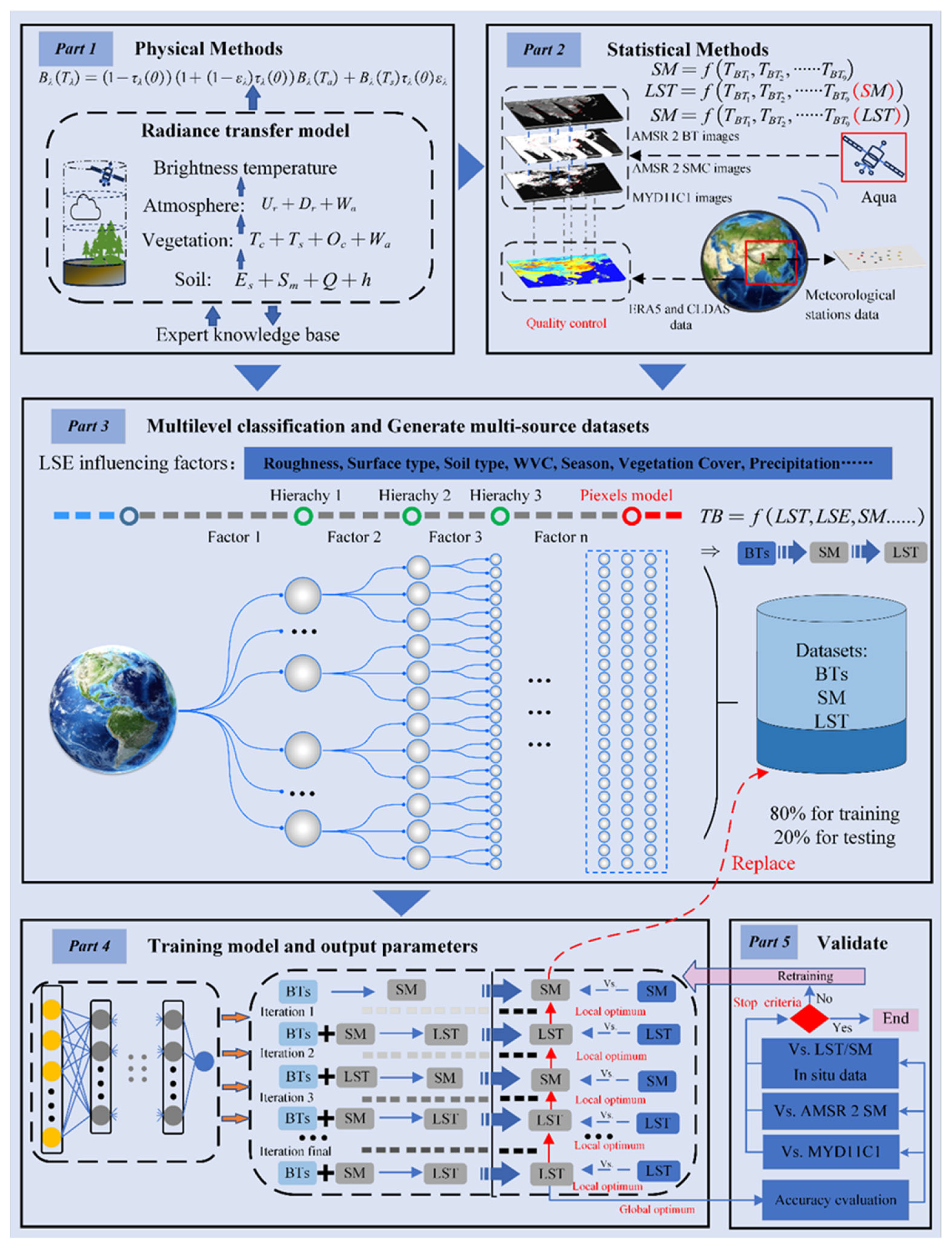
2. Methodology
3. Data and Method
3.1. Data
3.1.1. Remote Sensing Data
3.1.2. Simulation Data of AIEM and M-D
3.1.3. Assimilation Data and Ground Data
3.2. Geophysical Logic Derivation
3.2.1. Smooth Surface Radiative Model
3.2.2. Rough Surface Radiation Model
3.2.3. Vegetation Radiation Model
3.3. Multi-Hierarchy Classification and Establishment of a Multi-Source Database
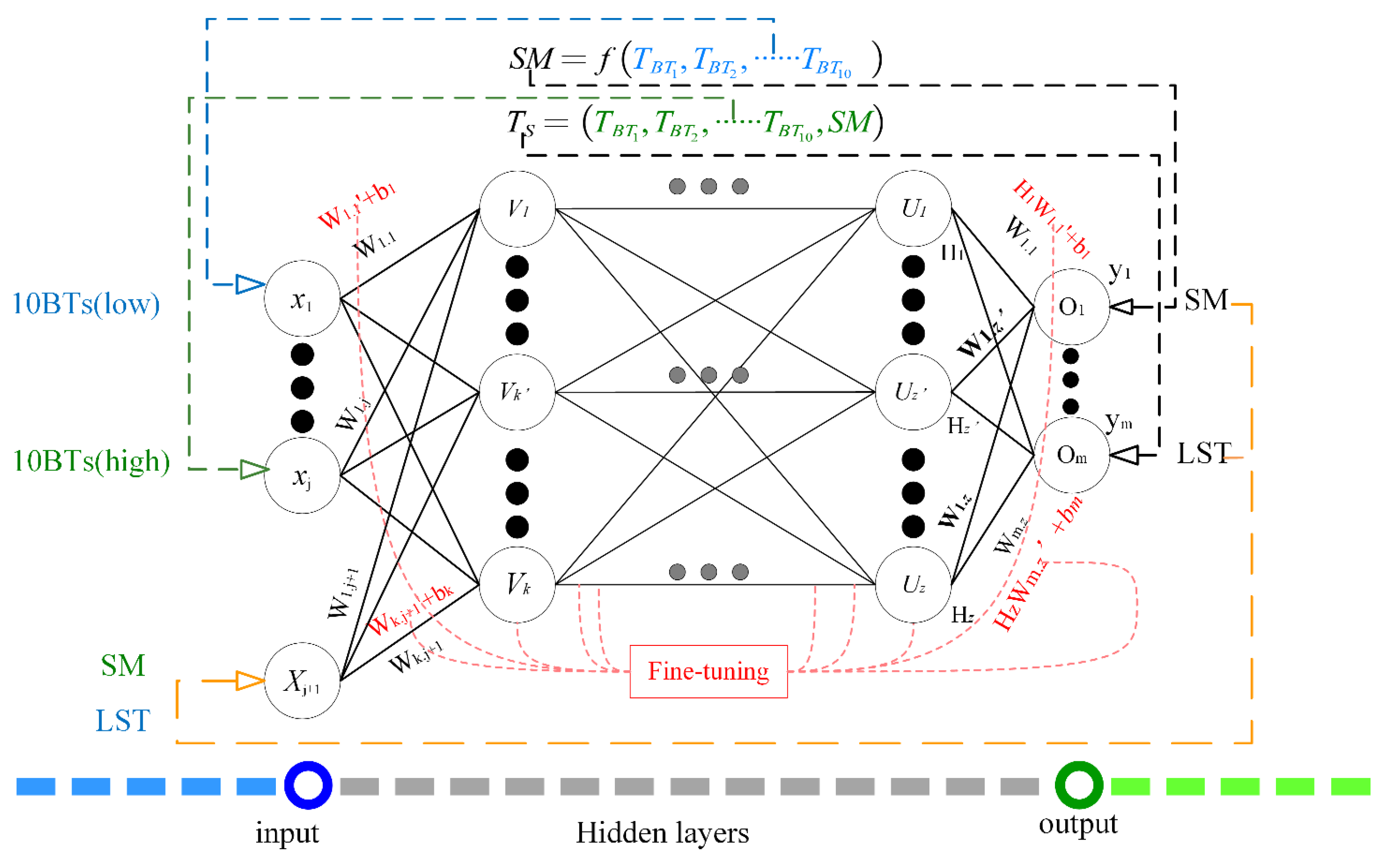
3.4. Neural Network Models with Mutually Prior Knowledge
3.4.1. Construct an Iterative Retrieval Model
3.4.2. The SM and LST Retrieval Method with Nested Large–Small Models
3.5. Validation Method
4. Results and Discussion
4.1. Case Study and Retrieval Scheme
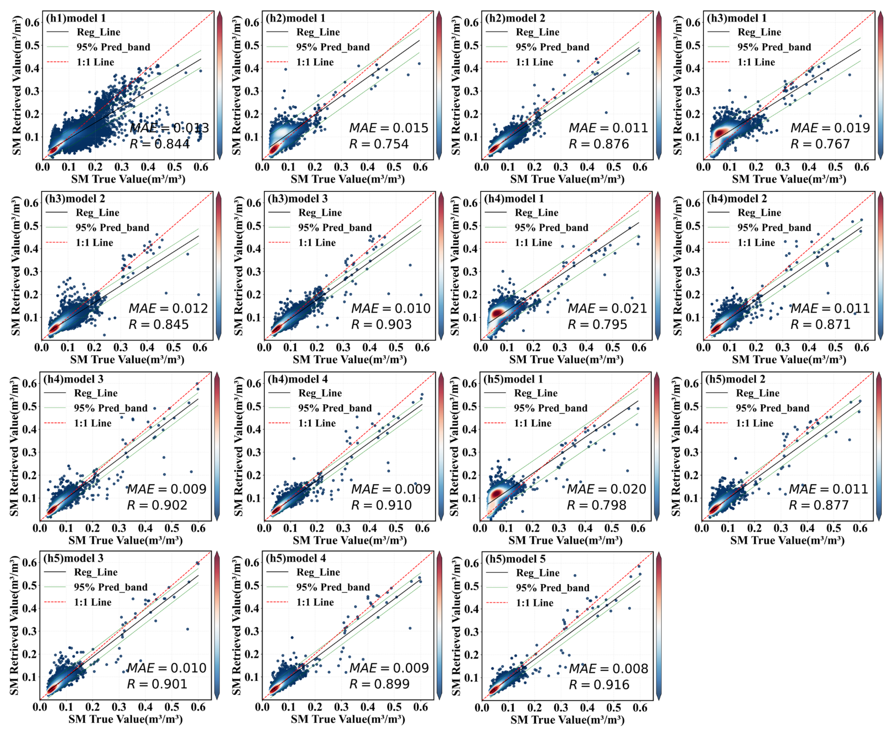
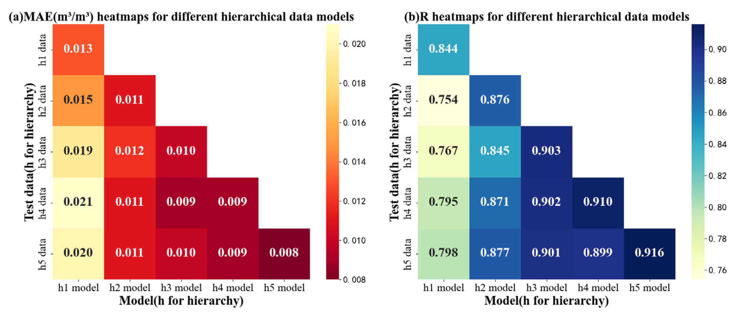
4.2. Large–Small Model Training and Testing
4.2.1. Ascending Orbit Iterative Retrieval Based on LST and SM as Prior Knowledge
4.2.2. Descending Orbit Iterative Retrieval Based on LST and SM as Prior Knowledge
4.3. Application and Validation
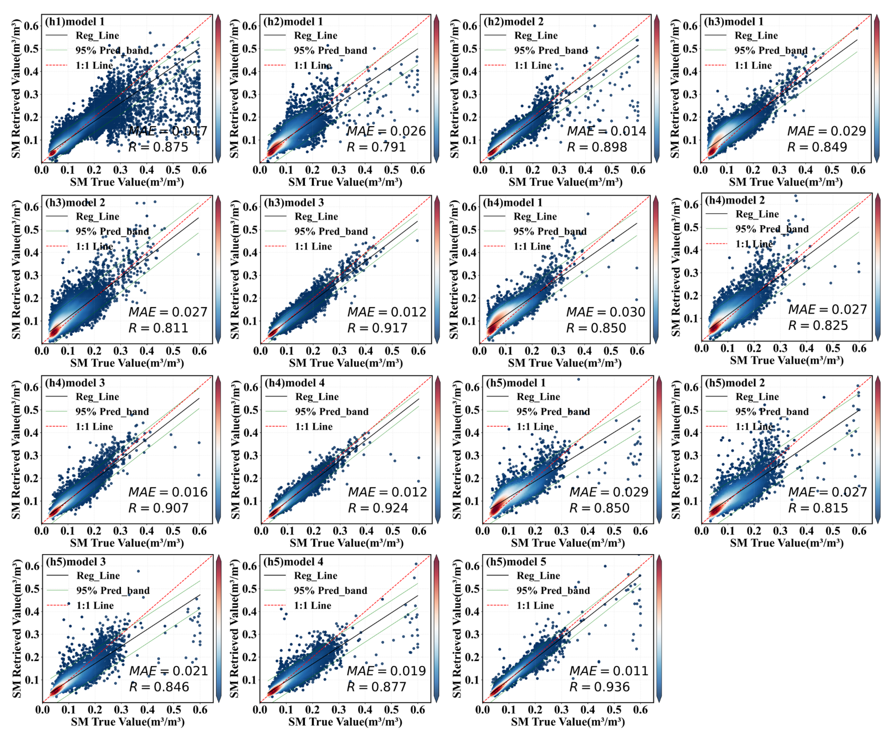
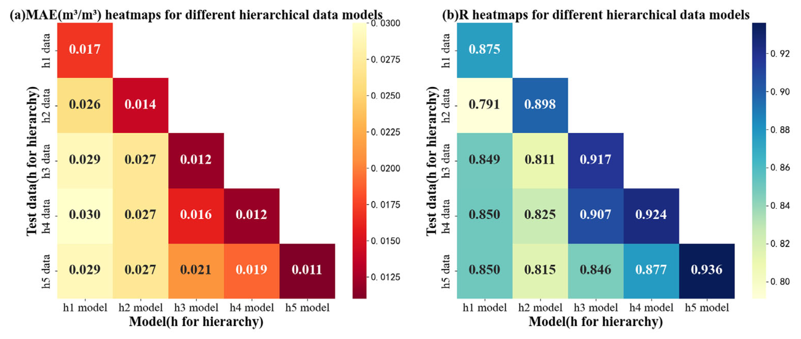
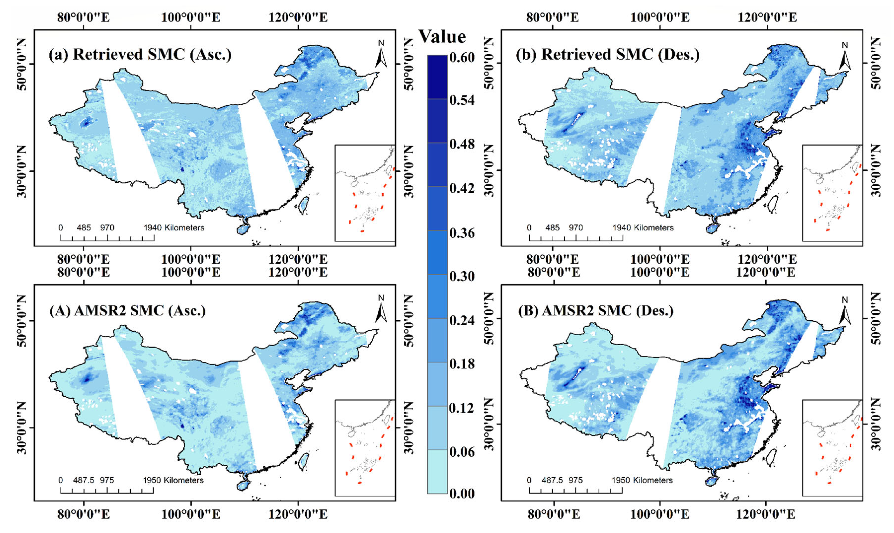
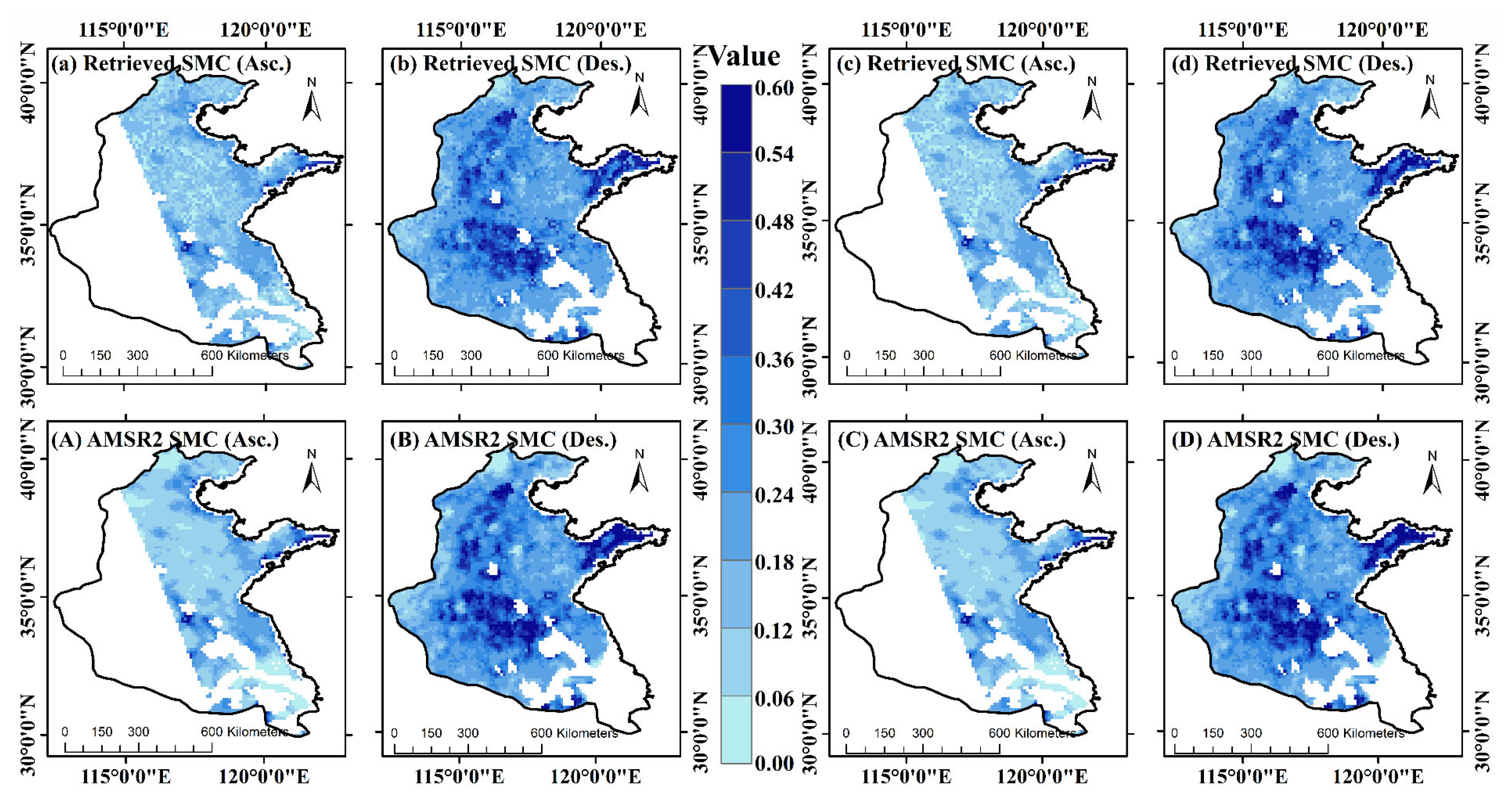
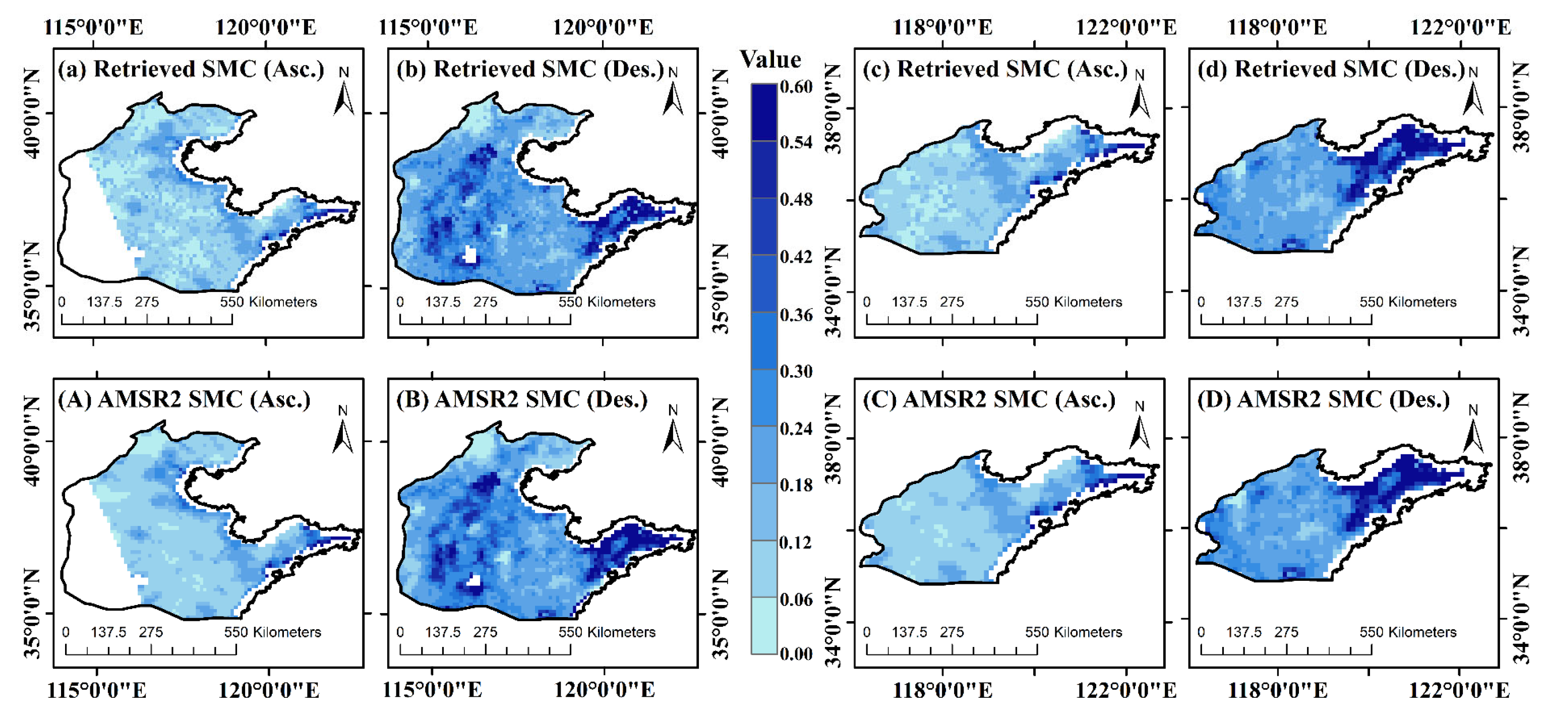
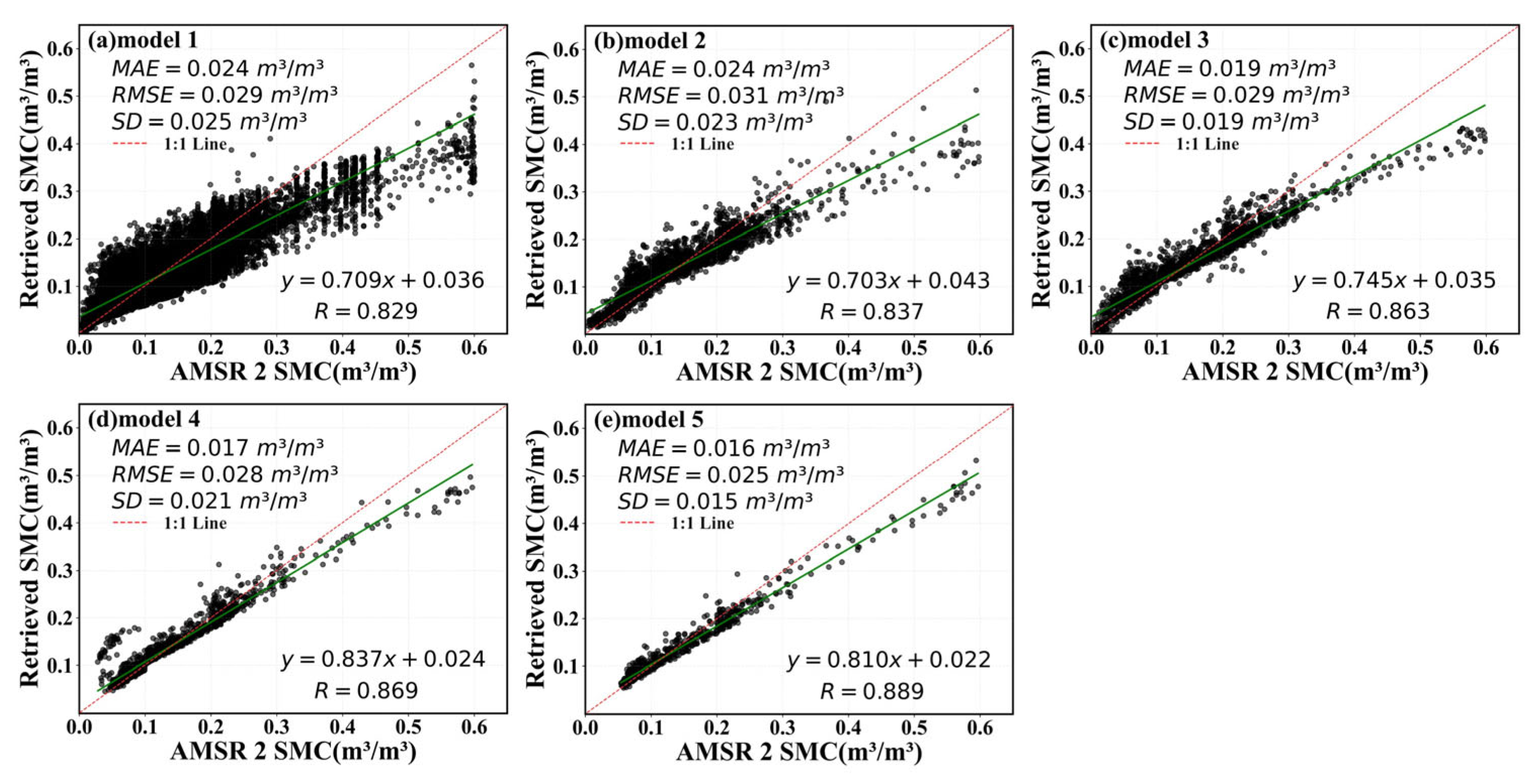
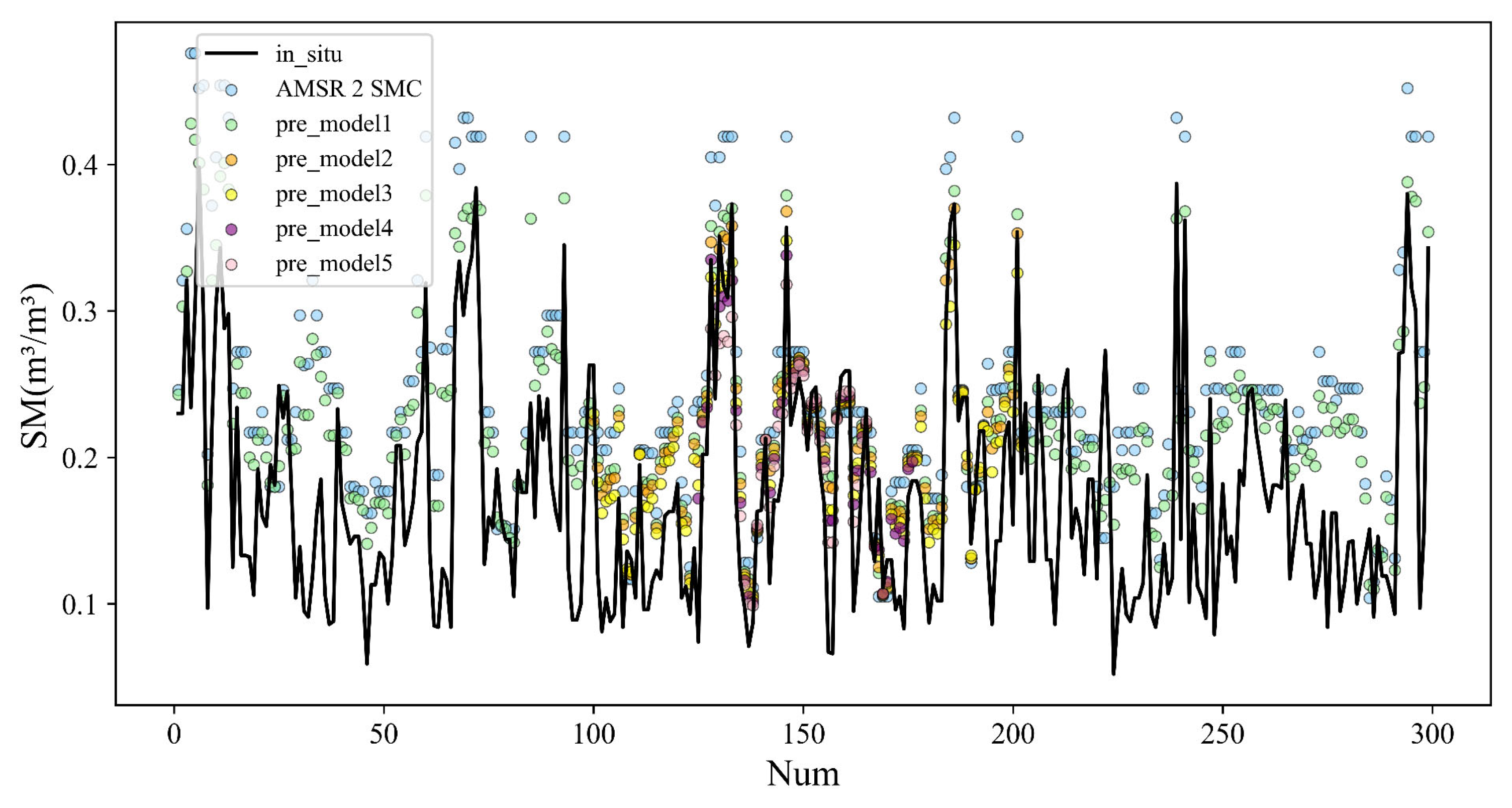
4.3.1. Application and Cross-Validation of SM Retrieval
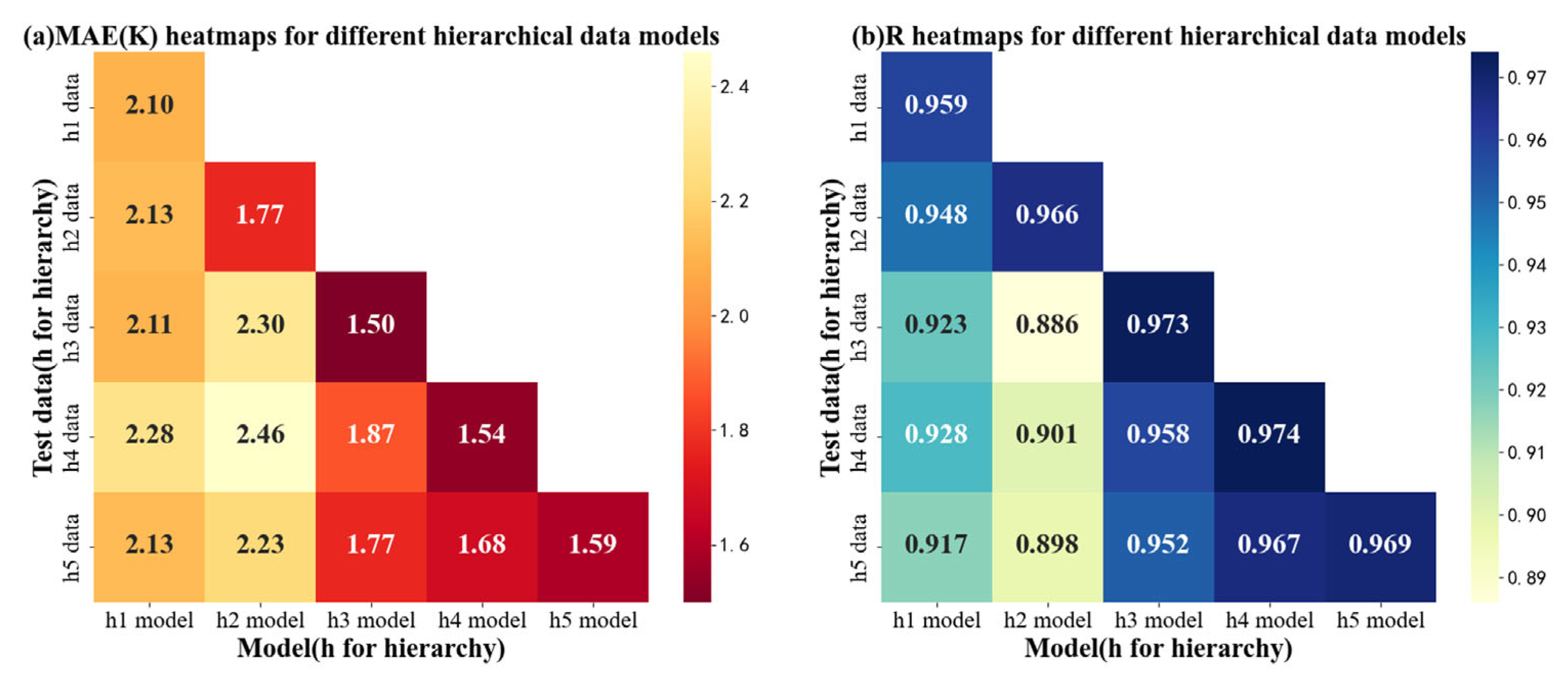
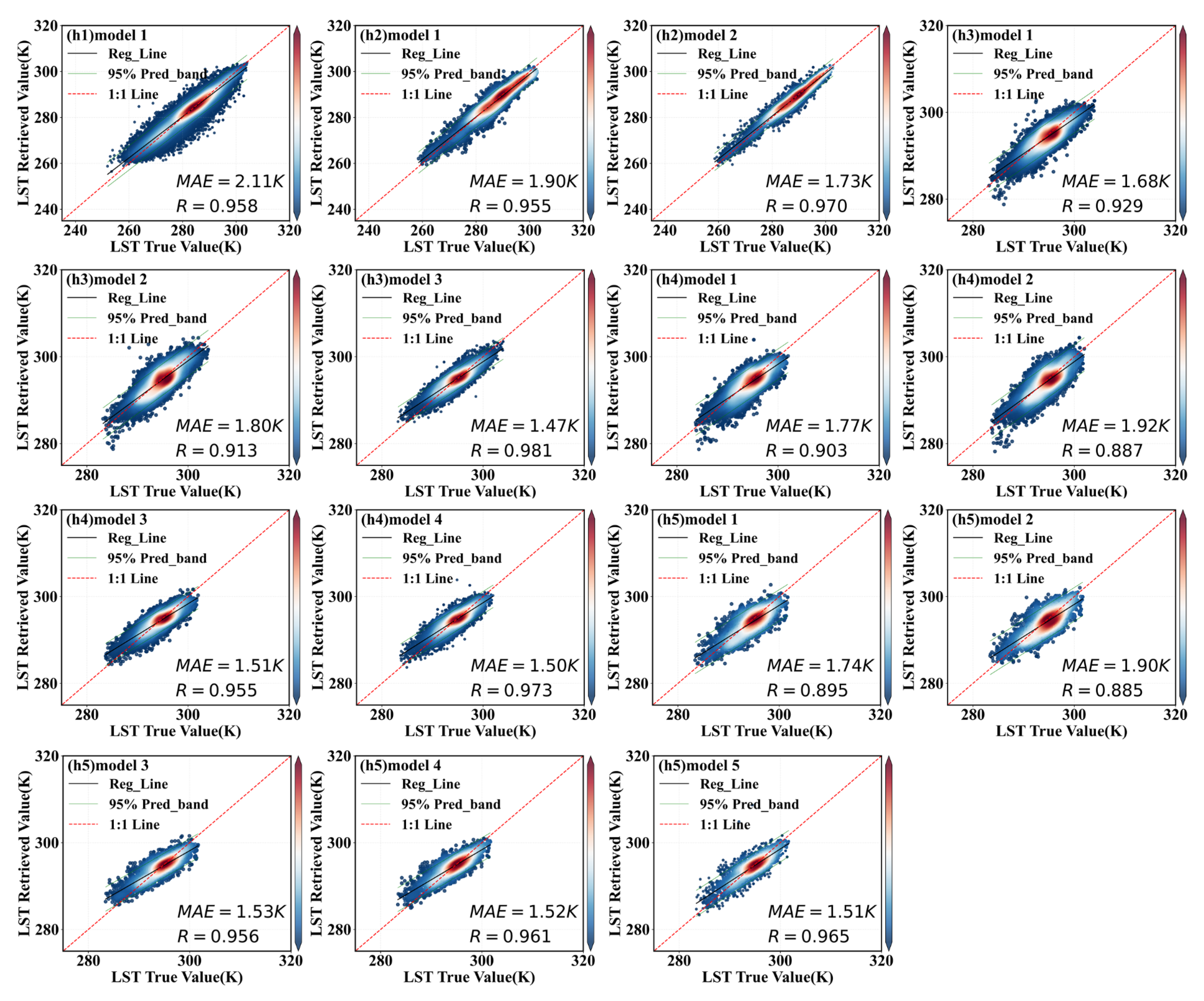
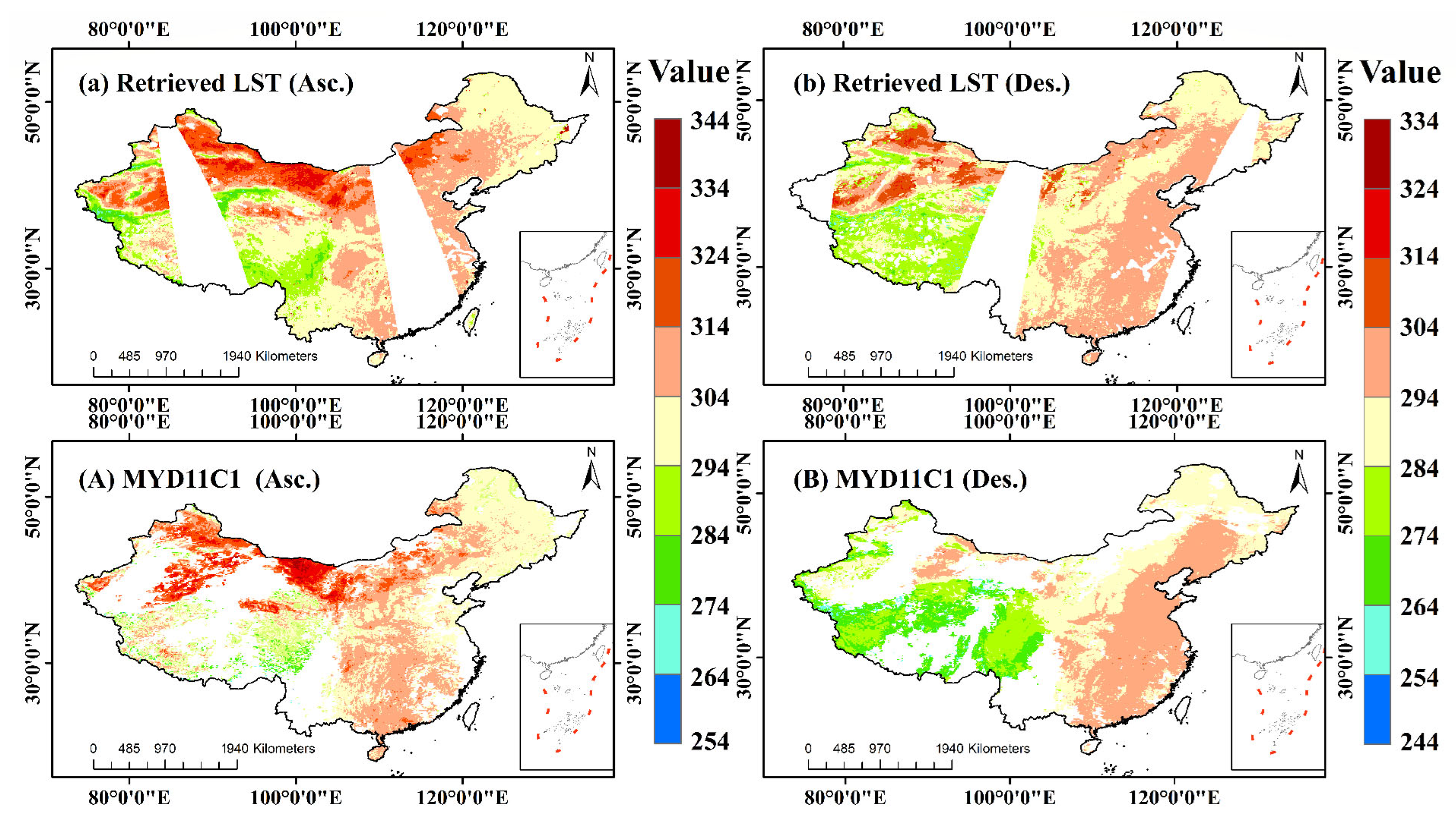
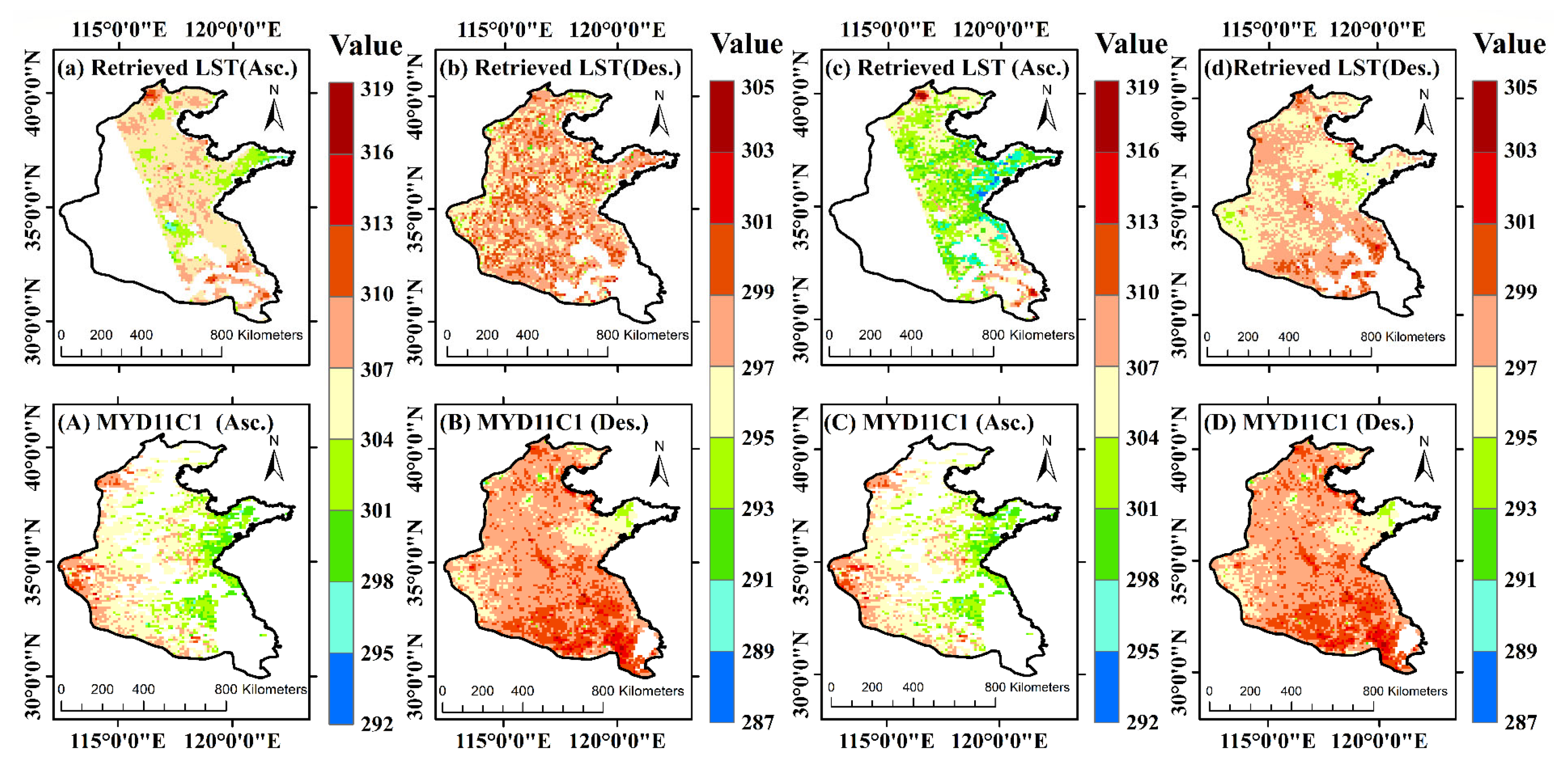
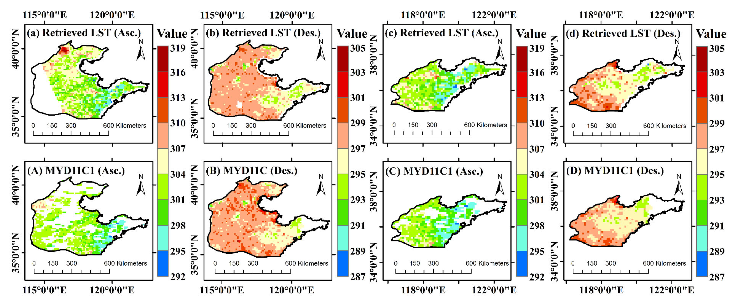
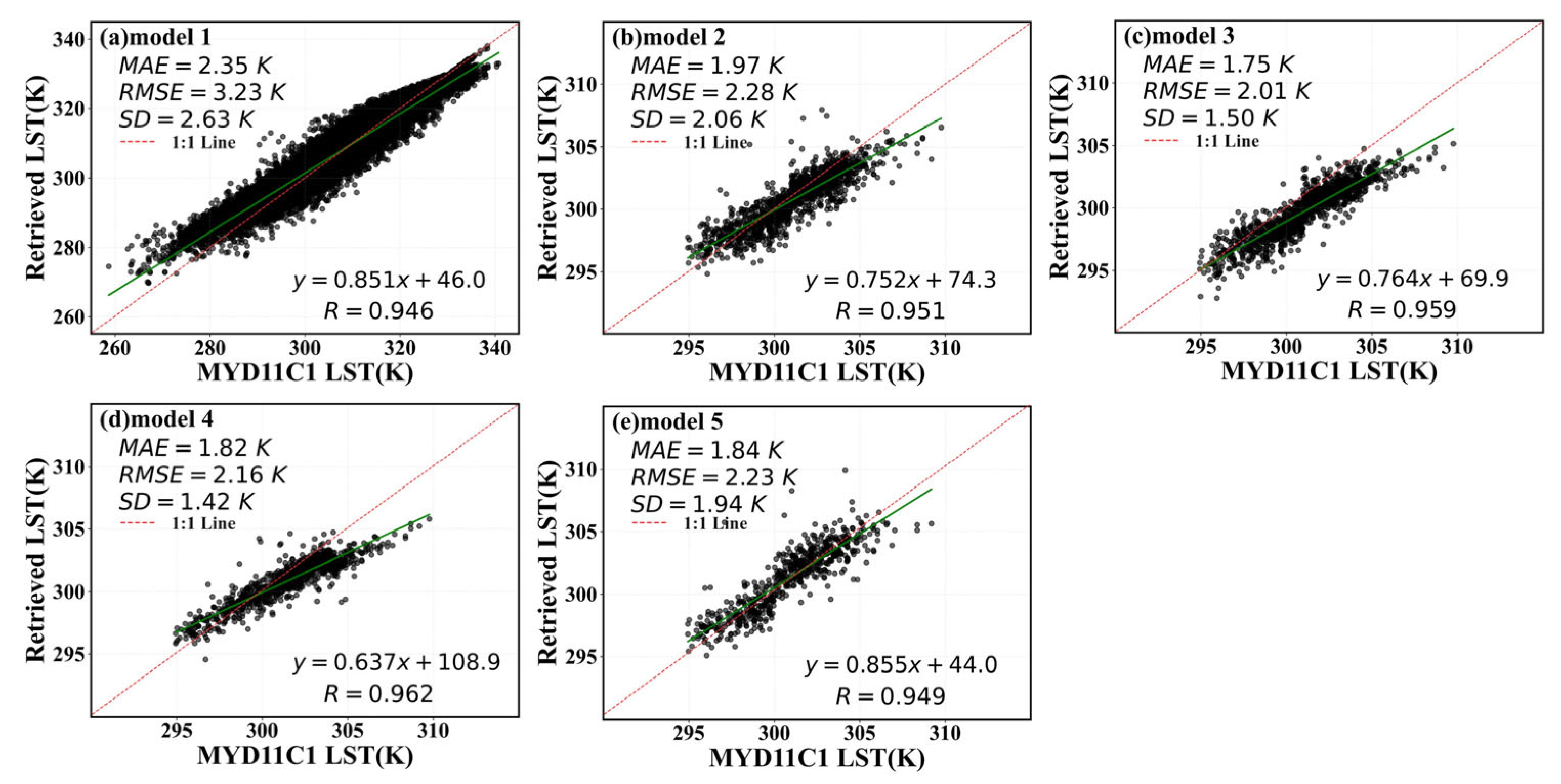
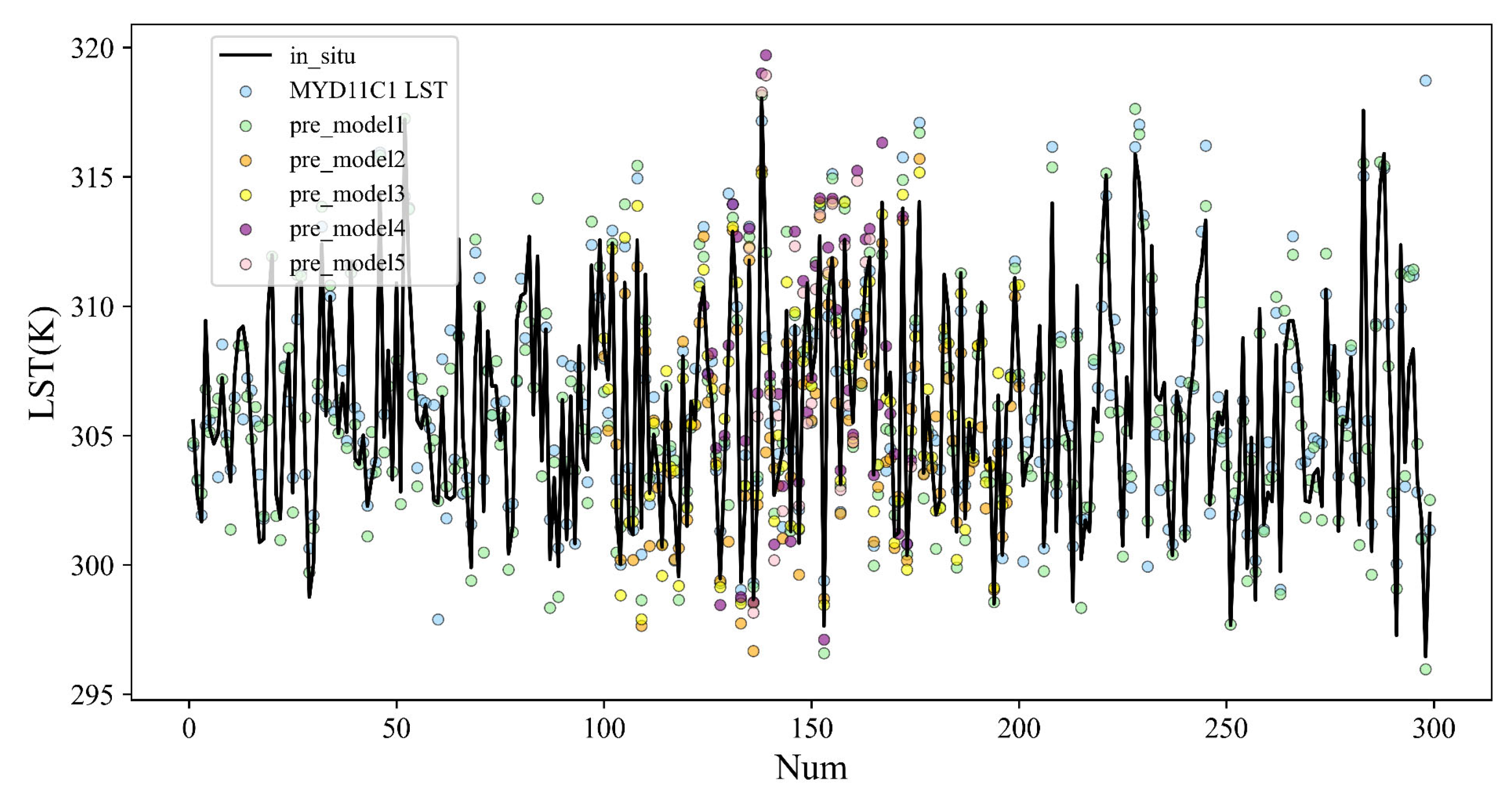
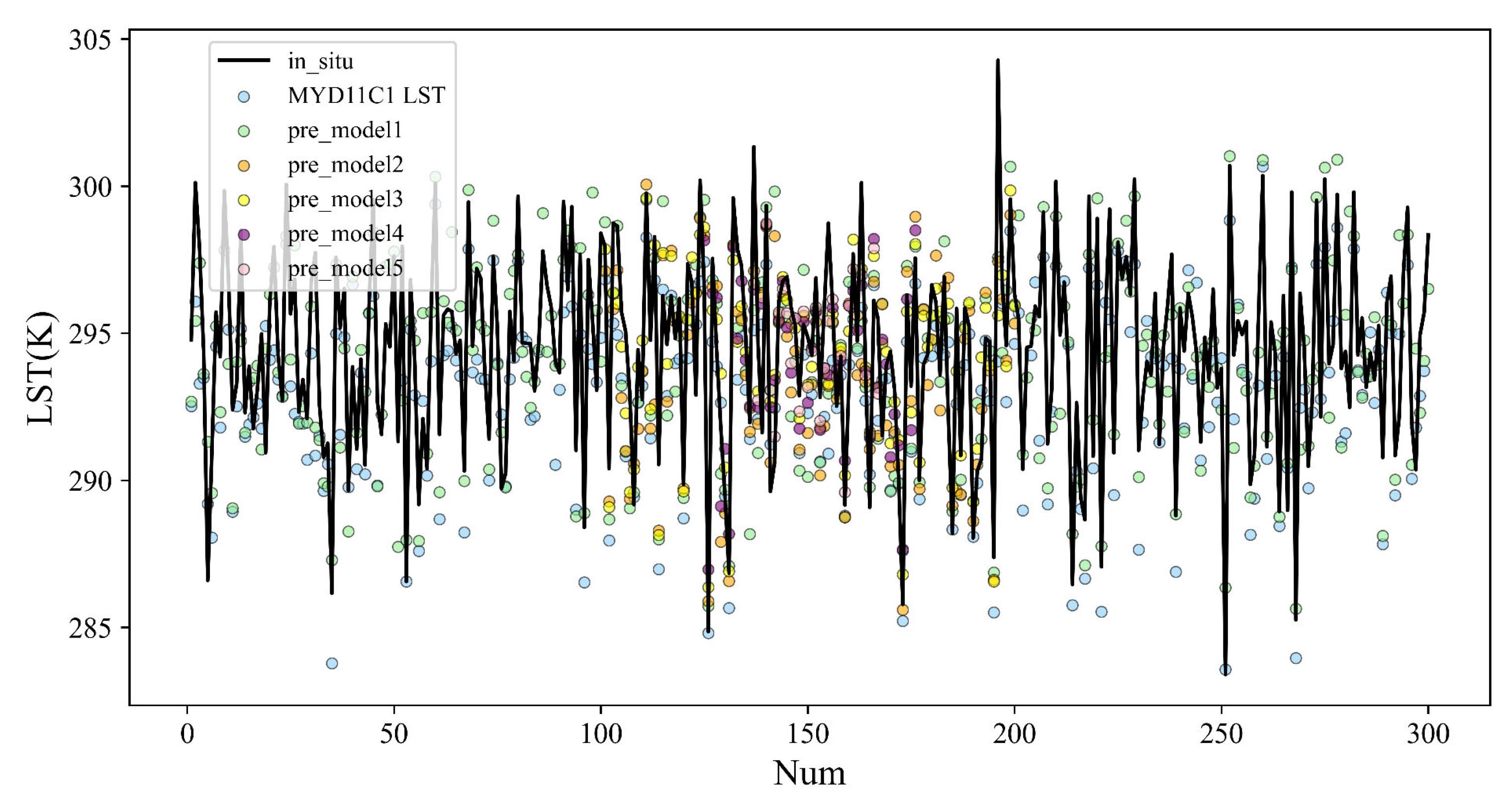
4.3.2. Application and Cross-Validation of LST Retrieval
4.3.3. Ground Validation
5. Conclusions and Future Prospects
Author Contributions
Funding
Data Availability Statement
Acknowledgments
Conflicts of Interest
References
- Duan, S.; Han, X.; Huang, C.; Li, Z.; Wu, H.; Qian, Y.; Gao, M.; Leng, P. Land Surface Temperature Retrieval from Passive Microwave Satellite Observations: State-of-the-Art and Future Directions. Remote Sens. 2020, 12, 2573. [Google Scholar] [CrossRef]
- Meng, X.; Mao, K.; Meng, F.; Shen, X.; Xu, T.; Cao, M. Long-Term Spatiotemporal Variations in Soil Moisture in North East China Based on 1-km Resolution Downscaled Passive Microwave Soil Moisture Products. Sensors 2019, 19, 3527. [Google Scholar] [CrossRef]
- Mao, K.; Shi, J.; Tang, H.; Guo, Y.; Qiu, Y.; Li, L. A Neural-Network Technique for Retrieving Land Surface Temperature from AMSR-E Passive Microwave Data. In Proceedings of the 2007 IEEE International Geoscience and Remote Sensing Symposium (IGARSS), Barcelona, Spain, 23–27 July 2007; IEEE: New York, NY, USA; pp. 4422–4425. [Google Scholar] [CrossRef]
- Yuan, Z.; NourEldeen, N.; Mao, K.; Qin, Z.; Xu, T. Spatiotemporal Change Analysis of Soil Moisture Based on Downscaling Technology in Africa. Water 2022, 14, 74. [Google Scholar] [CrossRef]
- Liou, Y.A.; Liu, S.F.; Wang, W.J. Retrieving Soil Moisture from Simulated Brightness Temperatures by a Neural Network. IEEE Trans. Geosci. Remote Sens. 2001, 39, 1662–1672. [Google Scholar] [CrossRef]
- Njoku, E.G.; Chan, S.K. Vegetation and Surface Roughness Effects on AMSR-E Land Observations. Remote Sens. Environ. 2006, 100, 190–199. [Google Scholar] [CrossRef]
- Jones, M.O.; Jones, L.A.; Kimball, J.S.; McDonald, K.C. Satellite Passive Microwave Remote Sensing for Monitoring Global Land Surface Phenology. Remote Sens. Environ. 2011, 115, 1102–1114. [Google Scholar] [CrossRef]
- Kerr, Y.H.; Njoku, E.G. A Semiempirical Model for Interpreting Microwave Emission from Semiarid Land Surfaces as Seen from Space. IEEE Trans. Geosci. Remote Sens. 1990, 28, 384–393. [Google Scholar] [CrossRef]
- Choudhury, B.J.; Schmugge, T.J.; Chang, A.; Newton, R.W. Effect of Surface Roughness on the Microwave Emission from Soils. J. Geophys. Res. 1979, 84, 5699–5706. [Google Scholar] [CrossRef]
- Jackson, T.J.; Schmugge, T.J. Vegetation Effects on the Microwave Emission of Soils. Remote Sens. Environ. 1991, 36, 203–212. [Google Scholar] [CrossRef]
- De Jeu, R.A.M.; Owe, M. Further Validation of a New Methodology for Surface Moisture and Vegetation Optical Depth Retrieval. Int. J. Remote Sens. 2003, 24, 4559–4578. [Google Scholar] [CrossRef]
- Meesters, A.G.C.A.; DeJeu, R.A.M.; Owe, M. Analytical Derivation of the Vegetation Optical Depth from the Microwave Polarization Difference Index. IEEE Geosci. Remote Sens. Lett. 2005, 2, 121–123. [Google Scholar] [CrossRef]
- Jiang, H.; Chen, S.; Li, X.; Wu, J.; Zhang, J.; Wu, L. A Novel Method for Long Time Series Passive Microwave Soil Moisture Downscaling over Central Tibet Plateau. Remote Sens. 2022, 14, 2902. [Google Scholar] [CrossRef]
- Huang, C.; Li, X.; Gu, J. Estimation of Regional Soil Moisture by Assimilating Multi-Sensor Passive Microwave Remote Sensing Observations based on Ensemble Kalman Filter. In Proceedings of the IGARSS 2008—2008 IEEE International Geoscience and Remote Sensing Symposium, Boston, MA, USA, 7–11 July 2008; IEEE: New York, NY, USA; pp. 1052–1055. [Google Scholar] [CrossRef]
- Del Frate, F.; Ferrazzoli, P.; Schiavon, G. Retrieving Soil Moisture and Agricultural Variables by Microwave Radiometry Using Neural Networks. Remote Sens. Environ. 2003, 84, 174–183. [Google Scholar] [CrossRef]
- Chai, S.; Goh, K.; Chang, Y.; Sim, K. Coupling Normalization with Moving Window in Backpropagation Neural Network (BNN) for Passive Microwave Soil Moisture Retrieval. Int. J. Comput. Intell. Syst. 2021, 14, 179. [Google Scholar] [CrossRef]
- Hu, Z.; Xu, L.; Yu, B. Soil Moisture Retrieval Using Convolutional Neural Networks: Application to Passive Microwave Remote Sensing. Int. Arch. Photogramm. Remote Sens. Spatial Inf. Sci. 2018, XLII–3, 583–586. [Google Scholar] [CrossRef]
- Li, D.; Hou, W.; Xu, J. AMSR-E Soil Moisture Inversion Based on GRNN Neural Network. In Proceedings of the 2020 7th International Forum on Electrical Engineering and Automation (IFEEA), Hefei, China, 25–27 September 2020; IEEE: New York, NY, USA, 2020; pp. 696–699. [Google Scholar] [CrossRef]
- Mao, K.; Wang, H.; Shi, J.; Heggy, E.; Wu, S.; Bateni, S.M.; Du, G. A General Paradigm for Retrieving Soil Moisture and Surface Temperature from Passive Microwave Remote Sensing Data Based on Artificial Intelligence. Remote Sens. 2023, 15, 1793. [Google Scholar] [CrossRef]
- Cao, M.; Mao, K.; Sayed, M.B.; Jun, C.; Shi, J.; Du, Y.; Du, G. Granulation-based LSTM-RF Combination Model for Hourly Sea Surface Temperature Prediction. Int. J. Digit. Earth 2023, 16, 3838–3859. [Google Scholar]
- Fily, M. A Simple Retrieval Method for Land Surface Temperature and Fraction of Water Surface Determination from Satellite Microwave Brightness Temperatures in Sub-Arctic Areas. Remote Sens. Environ. 2003, 85, 328–338. [Google Scholar] [CrossRef]
- Zhao, E.; Gao, C.; Jiang, X.; Liu, Z. Land Surface Temperature Retrieval from AMSR-E Passive Microwave Data. Opt. Express 2017, 25, A940. [Google Scholar] [CrossRef]
- Chen, S.; Chen, X.; Chen, W.; Su, Y.; Li, D. A Simple Retrieval Method of Land Surface Temperature from AMSR-E Passive Microwave Data—A Case Study over Southern China during the Strong Snow Disaster of 2008. Int. J. Appl. Earth Obs. Geoinf. 2011, 13, 140–151. [Google Scholar] [CrossRef]
- Gao, C.; Jiang, X.; Qian, Y.; Qiu, S.; Ma, L.; Li, Z. A Neural Network Based Method for Land Surface Temperature Retrieval from AMSR-E Passive Microwave Data. In Proceedings of the 2013 IEEE International Geoscience and Remote Sensing Symposium (IGARSS), Melbourne, VIC, Australia, 21–26 July 2013; IEEE: New York, NY, USA; pp. 469–472. [Google Scholar] [CrossRef]
- Shwetha, H.R.; Kumar, D.N. Prediction of Land Surface Temperature Under Cloudy Conditions Using Microwave Remote Sensing and ANN. Aquat. Procedia 2015, 4, 1381–1388. [Google Scholar] [CrossRef]
- Tan, J.; NourEldeen, N.; Mao, K.; Shi, J.; Li, Z.; Xu, T.; Yuan, Z. Deep Learning Convolutional Neural Network for the Retrieval of Land Surface Temperature from AMSR2 Data in China. Sensors 2019, 19, 2987. [Google Scholar] [CrossRef]
- Wang, S.; Zhou, J.; Lei, T.; Wu, H.; Zhang, X.; Ma, J.; Zhong, H. Estimating Land Surface Temperature from Satellite Passive Microwave Observations with the Traditional Neural Network, Deep Belief Network, and Convolutional Neural Network. Remote Sens. 2020, 12, 2691. [Google Scholar] [CrossRef]
- Fang, B.; Lakshmi, V.; Bindlish, R.; Jackson, T. AMSR2 Soil Moisture Downscaling Using Temperature and Vegetation Data. Remote Sens. 2018, 10, 1575. [Google Scholar] [CrossRef]
- Meng, X.; Yang, Y.; Zeng, J.; Peng, J.; Hu, J. Improvement of AMSR2 Soil Moisture Retrieval Using a Soil-Vegetation Temperature Decomposition Algorithm. IEEE Geosci. Remote Sens. Lett. 2022, 19, 2507805. [Google Scholar] [CrossRef]
- Song, P.; Huang, J.; Mansaray, L.R.; Wen, H.; Wu, H.; Liu, Z.; Wang, X. An Improved Soil Moisture Retrieval Algorithm Based on the Land Parameter Retrieval Model for Water–Land Mixed Pixels Using AMSR-E Data. IEEE Trans. Geosci. Remote Sens. 2019, 57, 7643–7657. [Google Scholar] [CrossRef]
- Mao, K.; Shi, J.; Li, Z.; Qin, Z.; Li, M.; Xu, B. A Physics-Based Statistical Algorithm for Retrieving Land Surface Temperature from AMSR-E Passive Microwave Data. Sci. China Ser. D Earth Sci. 2007, 50, 1115–1120. [Google Scholar] [CrossRef]
- Mao, K.; Ma, Y.; Xia, L.; Shen, X.; Sun, Z.; He, T.; Zhou, G. A Neural Network Method for Monitoring Snowstorm: A Case Study in Southern China. Chinese Geogr. Sci. 2014, 24, 599–606. [Google Scholar] [CrossRef]
- Wang, H.; Mao, K.; Shi, J.; Sayed, B.; Altantuya, D.; Sainbuyan, B.; Bao, Y. A normal form for synchronous land surface temperature and emissivity retrieval using deep learning coupled physical and statistical methods. Int. J. Appl. Earth Obs. Geoinf. 2024, 127, 103704. [Google Scholar] [CrossRef]
- Mao, K.; Wu, C.; Yuan, Z.; Liu, Y.; Cao, M.; Wang, H. Theory and Conditions for AI-Based Inversion Paradigm of Geophysical Parameters Using Energy Balance. Earth ArXiv 2024, 12, 1–26. [Google Scholar] [CrossRef]
- Bindlish, R.; Cosh, M.H.; Jackson, T.J.; Koike, T.; Fujii, H.; Chan, S.K.; Asanuma, J.; Berg, A.; Bosch, D.D.; Caldwell, T.; et al. GCOM-W AMSR2 Soil Moisture Product Validation Using Core Validation Sites. IEEE J. Sel. Top. Appl. Earth Obs. Remote Sens. 2018, 11, 209–219. [Google Scholar] [CrossRef]
- Kim, S.; Liu, Y.Y.; Johnson, F.M.; Parinussa, R.M.; Sharma, A. A Global Comparison of Alternate AMSR2 Soil Moisture Products: Why Do They Differ? Remote Sens. Environ. 2015, 161, 43–62. [Google Scholar] [CrossRef]
- Wan, Z.; Zhang, Y.; Zhang, Q.; Li, Z.-L. Quality Assessment and Validation of the MODIS Global Land Surface Temperature. Int. J. Remote Sens. 2004, 25, 261–274. [Google Scholar] [CrossRef]
- Huang, C.; Li, X.; Lu, L. Retrieving Soil Temperature Profile by Assimilating MODIS LST Products with Ensemble Kalman Filter. Remote Sens. Environ. 2008, 112, 1320–1336. [Google Scholar] [CrossRef]
- Son, N.; Chen, C.; Chen, C.; Chang, L.; Minh, V.Q. Monitoring Agricultural Drought in the Lower Mekong Basin Using MODIS NDVI and Land Surface Temperature Data. Int. J. Appl. Earth Obs. Geoinf. 2012, 18, 417–427. [Google Scholar] [CrossRef]
- Chen, K.; Wu, T.D.; Tsang, L.; Li, Q.; Shi, J.; Fung, A.K. Emission of Rough Surfaces Calculated by the Integral Equation Method with Comparison to Three-Dimensional Moment Method Simulations. IEEE Trans. Geosci. Remote Sens. 2003, 41, 90–101. [Google Scholar] [CrossRef]
- Shen, X.; Hong, Y.; Qin, Q.; Basara, J.B.; Mao, K.; Wang, D. A Semiphysical Microwave Surface Emission Model for Soil Moisture Retrieval. IEEE Trans. Geosci. Remote Sens. 2015, 53, 4079–4090. [Google Scholar] [CrossRef]
- Ferrazzoli, P.; Guerriero, L. Passive Microwave Remote Sensing of Forests: A Model Investigation. IEEE Trans. Geosci. Remote Sens. 1996, 34, 433–443. [Google Scholar] [CrossRef]
- Hersbach, H.; Bell, B.; Berrisford, P.; Hirahara, S.; Horányi, A.; Muñoz-Sabater, J.; Nicolas, J.; Peubey, C.; Radu, R.; Schepers, D.; et al. The ERA5 Global Reanalysis. Q. J. R. Meteorol. Soc. 2020, 146, 1999–2049. [Google Scholar] [CrossRef]
- Hoffmann, L.; Günther, G.; Li, D.; Stein, O.; Wu, X.; Griessbach, S.; Heng, Y.; Konopka, P.; Müller, R.; Vogel, B.; et al. From ERA-Interim to ERA5: The Considerable Impact of ECMWF’s Next-Generation Reanalysis on Lagrangian Transport Simulations. Atmos. Chem. Phys. 2019, 19, 3097–3124. [Google Scholar] [CrossRef]
- Olauson, J. ERA5: The New Champion of Wind Power Modelling? Renew. Energy 2018, 126, 322–331. [Google Scholar] [CrossRef]
- Fang, S.; Mao, K.; Xia, X.; Wang, P.; Shi, J.; Bateni, S.M.; Xu, T.; Cao, M.; Heggy, E. A Dataset of Daily Near-Surface Air Temperature in China from 1979 to 2018. Earth Syst. Sci. Data Discuss. 2022, 14, 1413–1432. [Google Scholar] [CrossRef]
- Dobson, M.; Ulaby, F.; Hallikainen, M.; El-rayes, M. Microwave Dielectric Behavior of Wet Soil—Part II: Dielectric Mixing Models. IEEE Trans. Geosci. Remote Sens. 1985, 23, 35–46. [Google Scholar] [CrossRef]
- Wang, J.R.; Choudhury, B.J. Remote Sensing of Soil Moisture Content Over Bare Fields at 1.4 GHz Frequency. J. Geophys. Res. Oceans 1981, 86, 5277–5282. [Google Scholar] [CrossRef]
- Mao, K.; Zuo, Z.; Shen, X.; Xu, T.; Gao, C.; Liu, G. Retrieval of Land-Surface Temperature from AMSR2 Data Using a Deep Dynamic Learning Neural Network. Chinese Geogr. Sci. 2018, 28, 1–11. [Google Scholar] [CrossRef]
- Wu, J.; Fang, J.; Tian, J. Terrain Representation and Distinguishing Ability of Roughness Algorithms Based on DEM with Different Resolutions. Int. J. Geo-Inf. 2019, 8, 180. [Google Scholar] [CrossRef]
- Njoku, E.G.; Li, L. Retrieval of Land Surface Parameters Using Passive Microwave Measurements at 6-18 GHz. IEEE Trans. Geosci. Remote Sens. 1999, 37, 79–93. [Google Scholar] [CrossRef]
- Shi, J.; Jackson, T.; Tao, J.; Du, J.; Bindlish, R.; Lu, L.; Chen, K. Microwave Vegetation Indices for Short Vegetation Covers from Satellite Passive Microwave Sensor AMSR-E. Remote Sens. Environ. 2008, 112, 4285–4300. [Google Scholar] [CrossRef]
- Jiang, L.; Shi, J.; Tjuatja, S.; Chen, K.S.; Du, J.; Zhang, L. Estimation of Snow Water Equivalent Using the Polarimetric Scanning Radiometer from the Cold Land Processes Experiments (CLPX03). IEEE Geosci. Remote Sens. Lett. 2011, 8, 359–363. [Google Scholar] [CrossRef]


| Data Type | Name | Source | Resolution |
|---|---|---|---|
| Remote Sensing Data | AMSR 2 BTs | Aqua (JAXA) | 0.1 Deg |
| AMSR 2 SMC | Aqua (JAXA) | 0.1 Deg | |
| MYD11C1 | Aqua (MODIS) | 0.05 Deg | |
| Simulation Data | AIEM Simulation Data | Advanced Integral Equation Model | |
| M-D Simulation Data | Matrix Doubling Model | ||
| Assimilation Data | ERA5 | ECMWF | 0.1 Deg |
| CLDAS | China Land Data Assimilation System | 0.0625 Deg | |
| Ground Data | Meteorological Station Data | National Meteorological Science Data Center | Point Data |
| Asc.SM Model (AF) | Asc.LST Model (AF) | Des.SM Model (AF) | Des.LST Model (AF) | |
|---|---|---|---|---|
| 1 | 32 (relu) | 64 (relu) | 32 (relu) | 64 (relu) |
| 2 | 416 (relu) | 648 (relu) | 448 (relu) | 680 (relu) |
| 3 | 880 (relu) | 612 (relu) | 624 (relu) | 688 (relu) |
| 4 | 640 (sigmoid) | 820 (relu) | 992 (sigmoid) | 804 (relu) |
| 5 | 1 (linear) | 982 (relu) | 1 (linear) | 992 (relu) |
| 6 | 748 (relu) | 970 (relu) | ||
| 7 | 820 (relu) | 860 (relu) | ||
| 8 | 1 (linear) | 1 (linear) |
| Ascending Orbits | Descending Orbits | |||||||||
|---|---|---|---|---|---|---|---|---|---|---|
| h1 | h2 | h3 | h4 | h5 | h1 | h2 | h3 | h4 | h5 | |
| Model 1 | 0.045 | 0.046 | 0.046 | 0.053 | 0.041 | 0.057 | 0.047 | 0.047 | 0.041 | 0.042 |
| Model 2 | \ | 0.046 | 0.046 | 0.045 | 0.035 | \ | 0.044 | 0.044 | 0.038 | 0.038 |
| Model 3 | \ | \ | 0.034 | 0.034 | 0.026 | \ | \ | 0.039 | 0.033 | 0.033 |
| Model 4 | \ | \ | \ | 0.031 | 0.027 | \ | \ | \ | 0.030 | 0.031 |
| Model 5 | \ | \ | \ | \ | 0.026 | \ | \ | \ | \ | 0.030 |
| AMSR 2 SM | 0.064 | 0.077 | 0.077 | 0.075 | 0.058 | 0.076 | 0.063 | 0.063 | 0.056 | 0.058 |
| Ascending Orbits | Descending Orbits | |||||||||
|---|---|---|---|---|---|---|---|---|---|---|
| h1 | h2 | h3 | h4 | h5 | h1 | h2 | h3 | h4 | h5 | |
| Model 1 | 2.30 | 2.03 | 2.03 | 2.10 | 2.34 | 2.12 | 2.04 | 2.04 | 2.07 | 2.21 |
| Model 2 | \ | 1.83 | 1.83 | 1.92 | 1.98 | \ | 1.95 | 1.95 | 1.96 | 1.96 |
| Model 3 | \ | \ | 1.71 | 1.70 | 1.72 | \ | \ | 1.79 | 1.84 | 1.78 |
| Model 4 | \ | \ | \ | 1.69 | 1.69 | \ | \ | \ | 1.79 | 1.76 |
| Model 5 | \ | \ | \ | \ | 1.67 | \ | \ | \ | \ | 1.72 |
| MYD11C1 | 2.61 | 2.34 | 2.34 | 2.33 | 2.24 | 2.56 | 2.38 | 2.38 | 2.34 | 2.28 |
Disclaimer/Publisher’s Note: The statements, opinions and data contained in all publications are solely those of the individual author(s) and contributor(s) and not of MDPI and/or the editor(s). MDPI and/or the editor(s) disclaim responsibility for any injury to people or property resulting from any ideas, methods, instructions or products referred to in the content. |
© 2025 by the authors. Licensee MDPI, Basel, Switzerland. This article is an open access article distributed under the terms and conditions of the Creative Commons Attribution (CC BY) license (https://creativecommons.org/licenses/by/4.0/).
Share and Cite
Liang, M.; Mao, K.; Shi, J.; Bateni, S.M.; Meng, F. An AI-Based Nested Large–Small Model for Passive Microwave Soil Moisture and Land Surface Temperature Retrieval Method. Remote Sens. 2025, 17, 1198. https://doi.org/10.3390/rs17071198
Liang M, Mao K, Shi J, Bateni SM, Meng F. An AI-Based Nested Large–Small Model for Passive Microwave Soil Moisture and Land Surface Temperature Retrieval Method. Remote Sensing. 2025; 17(7):1198. https://doi.org/10.3390/rs17071198
Chicago/Turabian StyleLiang, Mengjie, Kebiao Mao, Jiancheng Shi, Sayed M. Bateni, and Fei Meng. 2025. "An AI-Based Nested Large–Small Model for Passive Microwave Soil Moisture and Land Surface Temperature Retrieval Method" Remote Sensing 17, no. 7: 1198. https://doi.org/10.3390/rs17071198
APA StyleLiang, M., Mao, K., Shi, J., Bateni, S. M., & Meng, F. (2025). An AI-Based Nested Large–Small Model for Passive Microwave Soil Moisture and Land Surface Temperature Retrieval Method. Remote Sensing, 17(7), 1198. https://doi.org/10.3390/rs17071198