Evapotranspiration Disaggregation Using an Integrated Indicating Factor Based on Slope Units

Abstract

This study proposes an evapotranspiration (ET) disaggregation model based on slope units. Different slope units are first delineated based on digital elevation model data with high spatial resolution. Key factors influencing ET variability across topographies, such as radiation, vegetation, and moisture, are integrated using Sentinel-2 and DEM data to construct an indicating factor. A slope-scale ET disaggregation model is developed using ETWatch data (1 km resolution) and the integrated factor, yielding reliable 10 m resolution ET data that reflect slope-scale variations. The validation in Huairou and Baotianman shows coefficients of determination of 0.9 and 0.91, respectively, and root mean square errors of 0.45 mm and 0.47 mm. Compared to the original 1 km resolution ET data, the disaggregated results show improved accuracy, with R² values increasing by 1% (Huairou) and 2% (Baotianman) and RMSE decreasing by 21% and 13%, respectively. This model offers a novel approach for estimating forest evapotranspiration in mountainous areas and significant potential for water resource management and sustainable land–water allocation.

1. Introduction

Mountains cover approximately 27% of the Earth’s land surface, and roughly one-third of this area is forested, providing vital water resources that support over two billion people globally [1,2,3]. For this reason, mountainous regions are often referred to as natural “water towers”. In addition to their crucial role in water provision, forests in these areas offer a range of important ecosystem services, such as carbon sequestration, oxygen production, atmospheric purification, and biodiversity conservation [4,5,6]. These services contribute significantly to the overall ecological health of the planet and are essential to sustaining both local and global ecosystems.

Evapotranspiration (ET), which refers to the process of converting water from various underlying surfaces—such as water bodies, vegetation, and soils—into water vapor that is then transferred to the atmosphere, plays a central role in the global water cycle. It is estimated that approximately two-thirds of precipitation is returned to the atmosphere through ET [7]. This process is an integral component of the Earth’s water cycle, acting as a key link between ecological and hydrological processes. ET is also a critical indicator of vegetation health, agricultural productivity, and crop yields [8,9,10,11,12]. In mountainous regions, the study of regional ET models is essential for gaining a deeper understanding of the state and functionality of mountain ecosystems [13]. Furthermore, accurate estimations of evapotranspiration in mountainous areas are essential for guiding water management and allocation in these sensitive ecosystems [14,15].

While global ET datasets (e.g., MOD16, GLEAM, PML-V2) have advanced our understanding of water fluxes [16,17,18,19], their performance in mountainous regions remains problematic. Systematic biases have been reported in complex terrain due to (1) the topographic distortion of radiation budgets and turbulent fluxes [20,21], (2) the inadequate representation of elevation-driven microclimates [22,23], and (3) vegetation heterogeneity within coarse pixels [24,25]. These limitations persist despite improved spatial resolutions (1 km or finer resolution), as traditional pixel-based approaches fail to capture the fundamental hydrological units governing mountain ET dynamics.

To more accurately capture the spatial and temporal distribution patterns of ET in regions with complex topography, numerous researchers have developed remote sensing-based estimation models tailored for topographically diverse regions. First, net radiation serves as the energy source driving evapotranspiration (ET) processes, with solar radiation constituting the primary input component in energy balance calculations. Chen et al. (2013) achieved a mean solar radiation model error of −9.6 W/m² through three-component radiation modeling, outperforming traditional SEBS model results in sensible and latent heat flux estimations [26]. Further refinement by Liu et al. (2017) incorporated topographic shading factors into direct radiation calculations, yielding reliable model accuracy while preserving terrain-specific spatial patterns in radiation and ET outputs [27]. Next, terrain effects extend beyond radiation dynamics to influence critical ET parameters, including surface albedo, land surface temperature (LST), and aerodynamic properties. Zhao and Liu (2014) demonstrated slope-dominated ET variations in the Taihu Basin through localized zenith-angle corrections based on slope and aspect, revealing stronger slope impacts than elevation effects [28]. A comprehensive terrain correction framework developed by de Souza Lima and de Melo Ribeiro (2018) applied topographic normalization to albedo (empirical rotation model), elevation–LST regression, and slope-adjusted aerodynamic roughness in SEBAL modeling, reducing net radiation and ET estimation discrepancies by 64.3% and 75.9%, respectively, on shaded slopes [29]. Furthermore, the spatiotemporal extrapolation of meteorological data presents additional challenges in mountainous regions. While conventional approaches employ the spatial interpolation of station observations [30,31,32], sparse high-elevation stations necessitate terrain-integrated correction methods. Elevation-dependent temperature adjustments [33,34] and METRIC model enhancements incorporating elevation-corrected wind/pressure data exemplify such strategies [35]. Advanced approaches address multivariate influences on terrain, as demonstrated by Sun and Zhang’s (2016) nonlinear regression model spatializing temperature data using latitude, elevation, slope, and aspect parameters [36].

While the aforementioned approaches primarily focus on parameter-driven refinements within ET estimation frameworks, downscaling methods integrating existing coarse-resolution datasets have emerged as an alternative paradigm for high-spatial-resolution ET monitoring. This kind of method typically employs raster pixels as the basic unit of analysis. By using coarse-resolution evapotranspiration data along with key model parameters and integrating high-resolution remote sensing data, researchers can establish statistical relationships between high- and low-resolution data to perform the downscaling process [37,38,39,40]. However, this downscaling method often reveals “traces” along the boundaries of coarse-resolution pixels, where differences in pixel values lead to discrepancies in the downscaled results, especially near these boundaries. In particular, for surface types such as forests and croplands, areas with high internal homogeneity often form distinct spatial units. These units, characterized by similar vegetation types and environmental conditions, exhibit comparable ET characteristics. In the context of complex mountainous topography, such “spatially distributed units” correspond to slope units (SUs). These slope units can serve as more accurate and meaningful units for ET downscaling in mountainous regions, especially when topographical features complicate traditional pixel-based approaches. A slope unit is generally defined as an area enclosed by watershed and catchment lines, which are delineated according to the hydrological and geomorphological conditions of the region [41,42,43]. This geomorphologically realistic partitioning aligns with the natural boundaries of ecohydrological processes, providing a physically coherent framework for ET disaggregation. In mountainous areas with complex topography, various slope units can be identified, each exhibiting a higher degree of internal homogeneity compared to the heterogeneity observed between different slope units. Within a single slope unit, topographical features such as the slope gradient and slope direction are often consistent, leading to relatively homogeneous conditions within the unit. Meteorological factors, including air temperature, relative humidity, and wind speed, also tend to be more uniform within slope units. However, slope units with different topographical attributes exhibit significant differences in radiation [44], moisture conditions [45,46], vegetation landscape [47,48], and soil characteristics [49]. As such, the concept of slope unit-based monitoring is particularly well suited to mountainous areas where complex topography creates diverse ecological and hydrological conditions. Furthermore, by monitoring evapotranspiration at the slope scale, decision-makers and soil–water resource managers can develop more tailored and effective water management strategies for regions with varied terrain and landscape features.

In coarse-resolution raster pixels, the high heterogeneity of topographical features, moisture conditions, and vegetation types poses significant challenges for accurate evapotranspiration monitoring [50,51,52]. In terms of slope-scale ET monitoring, this study pursues three specific objectives: (1) delineate slope units as the basis for more precise downscaling, (2) develop an integrated indicator that reflects the differences in ET among different slope units, and (3) use this integrated indicator to disaggregate ET data based on slope units. These objectives aim to refine the monitoring of ET, providing more accurate spatial and temporal estimates that can inform better water management and contribute to sustainable development goals in forested regions with complex topography.

2. Materials and Methods

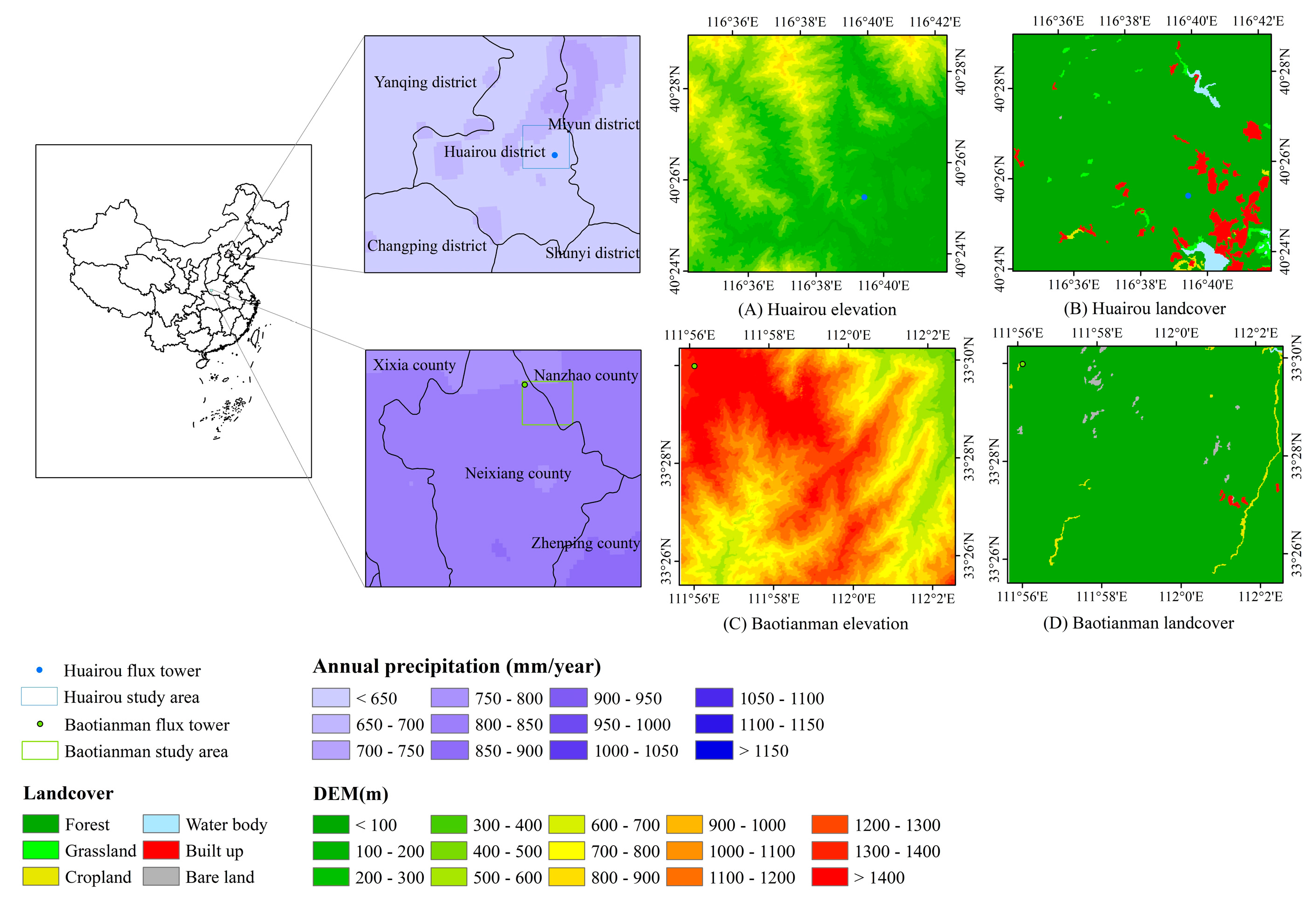
2.1. Study Area

In this study, we focus on two distinct areas: the Huairou Observatory in northeastern Beijing and the Baotianman Observatory in Neixiang County, Nanyang City, Henan Province (Figure 1). The study area covering approximately 10 square kilometers around the Huairou Observatory is characterized by a semi-arid and semi-humid temperate continental monsoon climate, which experiences four distinct seasons. This region is marked by simultaneous rainfall and heat during the summer, along with wet, hot summers and cold, snowless winters. In contrast, the Baotianman study area, also covering approximately 10 square kilometers, lies within the transition zone between the subtropical and temperate climate zones, and it is governed by a continental monsoon climate with clearly defined seasons. The Huairou Observatory is situated to the southeast of Huairou, at geographical coordinates 116°39′35″E and 40°25′22″N, with an elevation of 328 m above sea level. Meanwhile, the Baotianman Observatory is located in the northern part of Neixiang, with coordinates 111°56′07″E and 33°29′59″N, at an altitude of 1410.7 m.

2.2. Data Sources

This study primarily utilizes Sentinel-2 imagery, Fengyun geostationary satellite data, and TanDEM-X data as the main sources of remote sensing information. Additionally, in situ measurements, including eddy covariance (EC) data, radiation data, meteorological data, and ETWatch ET datasets, are incorporated. Detailed descriptions of these data sources are provided in the following sections.

2.2.1. Remote Sensing Data

Remote sensing data from Sentinel-2, the Fengyun geostationary satellites, and TanDEM-X were utilized in this study.

Sentinel-2 is capable of the high-resolution monitoring of the land surface and carries a multispectral imager (MSI) sensor that enables imaging at a high spatial resolution from 10 m to 60 m in visible, near-infrared-to-shortwave infrared bands. Sentinel-2 includes two successively launched 2A and 2B satellites, with an orbital altitude of 786 km and an imaging width of 290 km. The revisit period is 10 days for one satellite and 5 days for two complementary satellites. Sentinel-2 data can provide information on terrestrial vegetation growth [53,54,55], land cover conditions [56,57,58], and inland and coastal zone environments [59,60] and are the only satellite data that contain three bands within the red-edge wavelength range, which is very effective for monitoring vegetation health information [61,62]. Sentinel-2 surface reflectance data covering both study areas on clear days are processed and downloaded by Google Earth Engine (GEE, https://code.earthengine.google.com/, accessed on 24 June 2024).

The Fengyun-2 meteorological satellite (FY-2) is the first generation of geosynchronous orbit meteorological satellites developed by China, which complements the polar-orbiting meteorological satellite and constitutes China’s meteorological satellite application system. Its subsatellite point is 112°E, and the spatial resolution of the visible band data is 1.25 km. FY-2 is an important source of information for flood weather services, providing meteorological guarantees of major events and daily weather forecasts. In addition, FY-2 provides data support for meteorological, transportation, agriculture, fishery, ocean, environment, water conservancy, and forestry departments. Hourly cloud classification (CLC) data based on the FY-2F satellite acquired by the China National Satellite Meteorological Center (http://satellite.nsmc.org.cn/PortalSite/Default.aspx, accessed on 15 May 2024) are used to estimate sunshine hours [63].

The German TanDEM-X mission is a high-precision radar interferometry system using two TerraSAR-X satellites flying in formation from Deutsches Zentrum für Luft- und Raumfahrt (DLR, https://tandemx-science.dlr.de/, accessed on 16 May 2024). The first TerraSAR-X satellite was launched in 2007 with a planned lifetime of 5 years, and the second TerraSAR-X satellite was launched in 2009 with a planned lifetime of 5 years. The two satellites had a three-year work overlap period, during which DLR expected to generate a global high-precision DEM digital elevation model with an elevation positioning accuracy better than 2 m and a DEM grid spacing of 0.4 arcseconds (~12 m) [64].

All the remote sensing data were first converted to GeoTIFF format, processed to Albers equal-area conic projection, and resampled to 10 m spatial resolution. TanDEM-X data were utilized for the delineation of the slope units (introduced in Section 2.3.1), while TanDEM-X, FY-2F, and Sentinel-2 data were used together for the derivation of integrated indicating factors (introduced in Section 2.3.2).

2.2.2. In Situ Tower Observation Data

In situ observations from flux towers mainly consist of eddy covariance (EC) data. For EC observations, we collected observation data from the Huairou Observatory in 2020 from our lab and observation data from the Baotianman Observatory in 2019 from ChinaFlux (http://www.chinaflux.org/, accessed on 5 June 2024), which were mainly utilized to validate the integrated indicating factor (introduced in Section 3.3) and ET disaggregation results (introduced in Section 3.4). The instruments of the EC observation system mainly include an ultrasonic anemometer and a CO₂/H₂O infrared gas analyzer. The heights of the flux towers of Huairou and Baotianman stations were 40 m and 36 m, respectively, and the instruments were set up at 30 m and 29 m of the towers, respectively. The sampling frequency of EC observations was 10 Hz, and the average value was stored every 30 min. To match the flux source area of EC observations, the flux footprint prediction (FFP) model was applied in this study to calculate the footprint area of flux observations for subsequent use in the validation process of the evapotranspiration monitoring results [65] (Figure 2). For the validation process, the average ET within the footprint area was utilized for comparative analysis with the flux data. In Figure 2, the cross-shaped marker indicates the location of the flux tower, while the concentric red contour lines radiating outward represent the relative contribution percentages of the flux source area, ranging from 10% to 90%. The topographic information of the two flux towers and their respective footprint areas is summarized in

Table 1. Topographic information of flux tower and within-flux footprint.

Site	Elevation (m)	Slope (°)	Aspect	Proportions of Slopes with Different Aspect Within the Flux Tower Footprint Area (%)
				Sunny Slope	Shady Slope	Others
Huairou	328	22	Southeast	27.1	38.7	34.2
Baotianman	1410.7	18.1	West	22.6	47.5	29.9

. Since EC observations are often subject to energy balance non-closures, we performed energy balance corrections of the sensible and latent heat flux observations based on the Bowen ratio method [66]. In addition, when processing the collected EC data, we followed the study of Liu, et al. [67], including the process of removing data outliers, data before and after precipitation, and nighttime data under very low turbulent conditions (friction velocity below 0.2 m/s). EC data were missing for approximately 90 days from May to August 2020 due to instrument and data logger failures.

2.2.3. Meteorological Data

The meteorological data mainly include station observations of basic meteorological elements and radiation observations, which were obtained from the China Meteorological Information Service Center (https://data.cma.cn/, accessed on 9 April 2024). For the first part of the data, the meteorological parameters observed at each station mainly include relative air humidity (RH), wind speed (V_wind), atmospheric pressure (PRS), maximum temperature (T_max), minimum temperature (T_min), mean temperature (T_mean), and sunshine duration (sunt), and these point-scale observations are extrapolated to the spatial scale by combining the Kriging interpolation method [68]. For the four parameters T_max, T_min, T_mean, and PRS, the values at sea level are calculated based on the empirical relationships between these parameters and the elevation before spatial interpolation [35,69]. After interpolation, the values of all image elements at sea level are then extrapolated to the values at the corresponding elevations using the empirical relationships in conjunction with the digital elevation model data (DEM). All interpolated spatialized meteorological data are processed to Albers’ equal-area conic projection and resampled to 10 m spatial resolution. In addition, the second part of meteorological data includes radiation observations from the China International Exchange of Meteorological Radiation Data stations, which provide day-by-day radiation observations that mainly include total, direct, reflected, and scattered radiation. In this study, we use the data from the nearest radiation observation sites selected for the two study areas.

The above two parts of meteorological data are mainly used for the calculation of the net radiation in the integrated indicating factor.

2.2.4. ETWatch ET Data

The ETWatch ET dataset is mainly based on the idea of energy balance combined with the traditional P-M equation to calculate evapotranspiration. Several parametric models of key surface parameter integration are used to describe the surface heat fluxes by combining visible, near-infrared, thermal-infrared, and microwave remote sensing data, meteorological ground observations, atmospheric boundary layer data, and digital elevation model data [68]. Remote sensing data products, such as MODIS data (surface albedo, NDVI, and surface temperature) and geostationary meteorological satellite data, are specifically used in the calculation of evapotranspiration. ETWatch ET data products are developed at 1000 m spatial resolution and daily temporal resolution. The ETWatch model has been developed for more than 20 years and is widely used, achieving high validation accuracy and practical application effects in many regions in addition to guiding water resource management in corresponding regions [68,70,71].

2.3. Methods

In this study, an integrated indicating factor was constructed to reflect ET differences among slope units, incorporating radiation, vegetation, and moisture factors. Low-spatial-resolution ETWatch ET data are first disaggregated to yield slope-unit-based ET estimates using the integrated indicating factor and are subsequently downscaled to a 10 m resolution at the slope scale within each slope unit. Figure 3 summarizes the workflow for this study and presents the framework of the proposed ET disaggregation model based on slope units.

2.3.1. Delineation of Slope Units

This section of the study relies on TanDEM-X data with high spatial resolution, along with the hydrological analysis tools available in the ArcMap software 10.7 to delineate slope units. The primary approach involves extracting the watershed boundary from the filled DEM data and the catchment boundary from the inverted DEM data. The area enclosed by these two boundaries is defined as a slope unit. The specific steps in the process are outlined as follows.

First, the flow direction raster is calculated using depression-filled DEM data through the Flow Direction tool in ArcMap’s Hydrology Analysis Module. The flow accumulation raster is then derived using the Flow Accumulation tool. Using a raster calculator, river areas are assigned a value of 1 where the flow accumulation exceeds a certain threshold (1000 was selected based on preliminary testing), while all other areas are assigned a value of 0. This results in a raster representation of the river network. The Stream Link tool is then employed to calculate the starting and ending points of rivers within the network, using the river network raster and flow direction raster generated in the previous steps. Next, the Watershed tool is used to generate the watershed raster. The DEM data are inverted by subtracting the elevation values from the maximum elevation value using a raster calculator, followed by depression filling. The inverse DEM data are then processed using a similar procedure to generate the watershed raster. Both the watershed and reversed watershed rasters are subsequently converted to vector surfaces using the Raster to Polygon tool, representing the ridge line and valley line, respectively. The Union tool is applied to merge the watershed and reversed watershed polygons, yielding the preliminary delineation of the slope units. Through manual adjustments and the application of the Eliminate tool to merge fragmented patches, the final delineation of the slope units is achieved. A flow chart summarizing this process is provided in Figure 4.

2.3.2. Development of the Integrated Indicating Factor

To construct an integrated indicator reflecting evapotranspiration variability among slope units, it is necessary to use a method that combines radiation, vegetation, and moisture factors from the mechanistic method of ET calculation. The most widely applied mechanistic method is the Penman–Monteith (P-M) equation [72,73,74,75]. However, the P-M equation is relatively complex, involving several intricate parameters such as aerodynamic conductance and surface conductance, and its internal structure is nonlinear. In contrast, the Priestley–Taylor (P–T) equation, a simplified form of the P-M equation primarily driven by net radiation data, was selected to construct the integrated indicating factor in this study. The P–T equation is mainly used for the calculation of potential evapotranspiration. When actual evapotranspiration needs to be calculated, the P–T equation often needs to be corrected using restrictive functions based on vegetation and moisture factors, etc. [76,77], which are expressed in the equation as follows:

$${LE}_a={f_{c}f}_{vm}{f}_{sm}\alpha {\displaystyle \frac{△}{△+\gamma }}(R_n-G)$$

(1)

where ${LE}_a$ is the latent heat flux corresponding to the actual evapotranspiration, $f_c$ is the restrictive function of vegetation canopy cover, $f_{vm}$ is the restrictive function of vegetation canopy moisture, $f_{sm}$ is the restrictive function of soil moisture, $\alpha$ is the Priestley–Taylor coefficient, $△$ is the slope of the “saturation water vapor pressure–air temperature” curve, $\gamma$ is the psychrometric constant, $R_n$ is the net radiation, and $G$ is the soil heat flux. It is obvious that the restrictive functions and the other parameters are combined in the form of a simple product in the P–T equation, which is very suitable for the construction of an integrated indicating factor. The differences in the topographical characteristics lead to very different radiation conditions among different slope units, resulting in differences in vegetation landscape and soil moisture in different topographical conditions. The differences in these aspects can be expressed by net radiation and three restrictive functions of $f_c$, $f_{vm},$ and $f_{sm}$. Considering the situation of very sparsely distributed meteorological stations in the mountainous underlying surface, it is difficult to obtain spatially distributed meteorological data accurately in complex topographical conditions; thus, the meteorological parameters are disregarded here. At the same time, the soil heat flux (G) can be approximated to be 0 at the daily scale, so the P–T equation is simplified to construct the integrated indicating factor F (W/m²) reflecting the differences in evapotranspiration among the slope units, as shown in the following equation:

$$F=(1-N\left(FVC\right)N\left(GVMI\right)N\left(TWI\right))R_n$$

(2)

where N(f) stands for normalization of factor f, i.e., $N\left(f\right)={\displaystyle \frac{f-f_{min}}{f_{max}-f_{min}}}$, where $R_n$ (W/m²) is the net radiation considering the topographic conditions, N(FVC) represents the restrictive function of vegetation canopy cover by fractional vegetation cover (FVC), N(GVMI) represents the restrictive function of vegetation canopy moisture by the global vegetation moisture index (GVMI), and N(TWI) represents the restrictive function of soil moisture by the topographical moisture index (TWI). The details of these factors are described below.

$R_n,$ considering topographical effects at the daily scale, is mainly calculated with Sentinel-2 surface reflectance data and TanDEM-X data according to the following equations:

$$R_n=R_{s\downarrow }\left(1-\alpha \right)-R_{nl}$$

(3)

$$R_{s\downarrow }=R_{s\downarrow \_dir}+R_{s\downarrow \_dif}+R_{s\downarrow \_adj}$$

(4)

$$R_{s\downarrow \_dir}=R_{s\downarrow \_dir0}\times R_b$$

(5)

$$R_{s\downarrow \_dif}=R_{s\downarrow \_dif0}\times {\mathsf{\Phi }}_{sky}$$

(6)

$$R_{s\downarrow \_adj}=F_{ts}{\alpha }_m(R_{s\downarrow \_dir}+R_{s\downarrow \_dif})$$

(7)

$$R_{nl}=\sigma {\displaystyle \frac{T_{min}^4+T_{max}^4}{2}}(0.34-0.14\sqrt{e_a})(1.35{\displaystyle \frac{R_{s\downarrow }}{R_{s\downarrow 0}}}-0.35)$$

(8)

where $R_{s\downarrow }$ is the downward shortwave radiation, $\alpha$ is the surface albedo calculated based on the linear combination of multiband values of Sentinel-2 surface reflectance data, $R_{nl}$ is the net longwave radiation, $R_{s\downarrow \_dir}$ is the direct solar radiation, $R_{s\downarrow \_dir0}$ represents the direct solar radiation on a horizontal surface calibrated with in situ measured radiation and sunshine duration data, $R_b$ denotes the ratio of the direct solar radiation on an inclined surface to that on a horizontal surface, $R_{s\downarrow \_dif}$ is the sky diffuse radiation, $R_{s\downarrow \_dif0}$ represents the diffuse sky radiation on a horizontal surface, ${\mathsf{\Phi }}_{sky}$ is the sky view factor, $F_{ts}$ is the topographical structure factor, ${\alpha }_m$ is the average surface albedo, $\sigma$ is the Stefan–Boltzmann constant (4.903 × 10⁻⁹ MJ∙K⁻⁴∙m⁻²∙day⁻¹), $e_a$ is the actual vapor pressure, $T_{max}$ and $T_{min}$ are the daily maximum and minimum air temperatures, respectively, and $R_{s\downarrow 0}$ is the clear-sky solar radiation. Details of $R_n$ considering topographical factor calculations and the abovementioned parameters are described in the study by Wang et al. (2022) [20].

The FVC is calculated based on NDVI data with the following equations:

$$FVC={\displaystyle \frac{NDVI-{NDVI}_{max}}{{NDVI}_{max}-{NDVI}_{min}}}$$

(9)

$$NDVI={\displaystyle \frac{NIR-RED}{NIR+RED}}$$

(10)

where NDVI is the normalized difference vegetation index, ${NDVI}_{max}$ and ${NDVI}_{min}$ represent the NDVI values of vegetation (0.9) and soil (0.1), respectively, and NIR and RED denote the surface reflectance of the near-infrared band and the red band, respectively, corresponding to bands 8 and 4 of Sentinel-2 data.

The global vegetation moisture index (GVMI), which maximizes the sensitivity of the vegetation canopy moisture content while minimizing the effect of other influencing factors, such as atmospheric conditions, is calculated as follows [78,79]:

$$GVMI={\displaystyle \frac{(NIR+0.1)-(SWIR+0.02)}{\left(NIR+0.1\right)+(SWIR+0.02)}}$$

(11)

where NIR and SWIR represent the surface reflectance of the near-infrared band and the shortwave infrared band, respectively, corresponding to bands 8 and 12 of Sentinel-2 data. The FVC and GVMI are calculated using Sentinel-2 data on clear days and are then interpolated to a daily scale with the Savitzky–Golay (S-G) filtering method [80,81].

High-spatial-resolution soil moisture data are often difficult to obtain. The topographic moisture index (TWI) was found to correlate well with the spatial distribution of actual soil moisture at small watershed scales [82,83]. Therefore, here, TWI is used to describe the catchment trends of individual raster cells reflecting soil moisture under complex topographic conditions, which is calculated as follows:

$$TWI=\mathit{ln}\left({\displaystyle \frac{a}{\mathit{tan}b}}\right)$$

(12)

where a is the catchment area, and b is the slope. The catchment area (a) can be calculated by combining the intermediate results of the abovementioned slope unit delineation process.

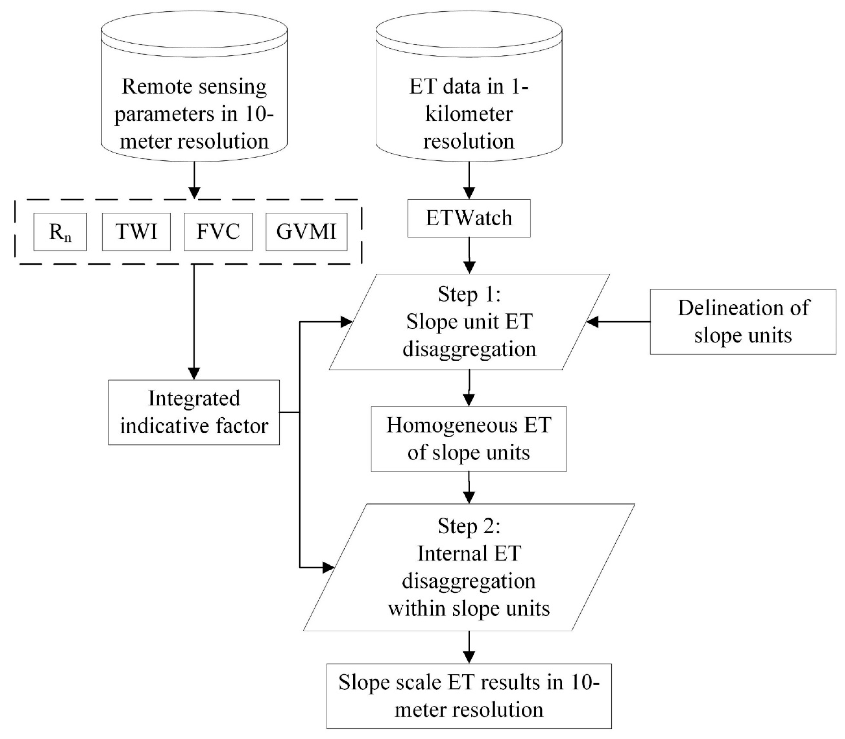
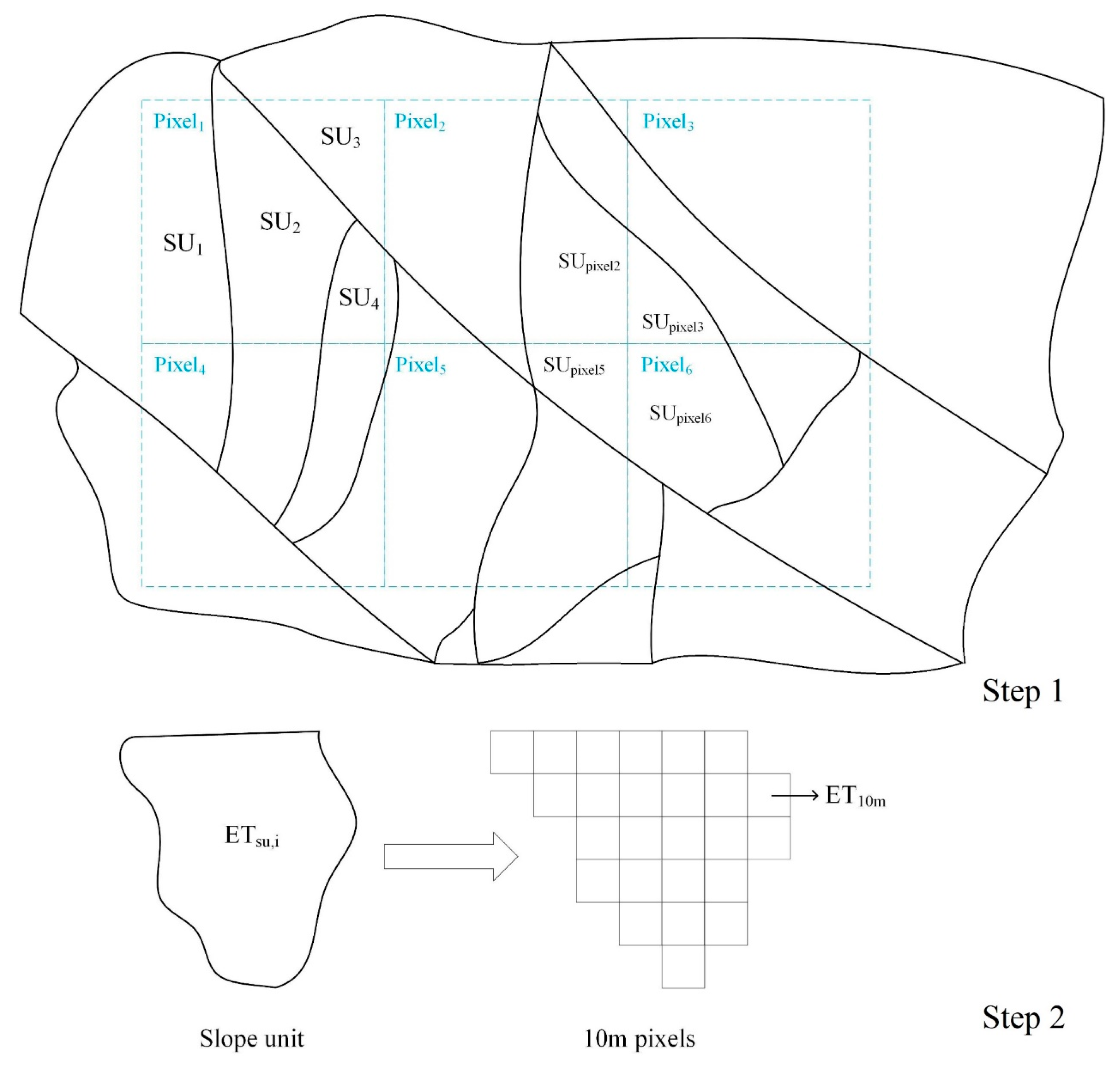
2.3.3. ET Disaggregation Method

Based on Sentinel 2 data and the TanDEM-X digital elevation model data, the integrated indicating factor reflecting the difference in evapotranspiration among slope units at a 10 m spatial resolution can be calculated by combining Equations (2)–(12). Following this, ETWatch ET data at a 1 km resolution can be disaggregated by combining the slope unit results and the integrated indicating factor constructed above. There are currently many coarse-resolution ET data products with different model accuracies in addition to ETWatch data. Here, we selected SSEBop data from the USGS [84] and FLDAS data from FEWS NET [85] and applied them to the ET disaggregation model developed in this research at Baotianman for comparative analysis. In practice, as shown in the schematic diagram of Step 1 in Figure 5, one coarse-resolution raster cell often contains multiple slope units, such as Pixel 1 marked by the blue dashed line containing four slope units SU1, SU2, SU3, and SU4. At the same time, there are also cases where one slope unit spans multiple coarse-resolution raster cells, such as the middle right slope unit spanning Pixel 2, Pixel 3, Pixel 5, and Pixel 6. In terms of the specific disaggregation process, the integrated indicating factor is utilized to reflect the difference in evapotranspiration among slope units, referring to the existing downscaling algorithm that uses the relationship between fine- and coarse-resolution influencing factors; that is, ${ET}_{su,i}:{ET}_{su,j}=F_{su,i}:F_{su,j}$. Thus, the ET relationship between fine and coarse-raster cells is established, and coarse-resolution ET can be disaggregated to the slope unit scale, as expressed in Equation (13) as follows:

$${\displaystyle \frac{{ET}_{su,i}}{{ET}_{coarse}}}={\displaystyle \frac{F_{su,i}}{F_{coarse}}}$$

(13)

where ${ET}_{su,i} \mathrm{a}\mathrm{n}\mathrm{d} {ET}_{su,j}$ represents slope units i and j; $F_{su,i} \mathrm{a}\mathrm{n}\mathrm{d} F_{su,j}$ represent the mean values of the integrated indicating factor within slope units i and j, respectively; ${ET}_{coarse}$ represents coarse-resolution ET data (represents ETWatch ET data at 1 km spatial resolution); and $F_{coarse}$ is the mean value of the integrated indicating factor within the 1 km spatial resolution raster cell. Based on the above, there are cases where one slope unit spans multiple coarse-resolution raster cells, and the disaggregated ET results from different coarse-resolution raster cells can be obtained according to Equation (6). Then, the weighted average of disaggregated ET results from different coarse-resolution raster cells was obtained with the area of the slope unit in different coarse-resolution raster cells as the weight, as shown in Equation (14):

$${ET}_{su,i}={\displaystyle \frac{\sum {ET}_{su,i in pixel,m}{S}_{su,i in pixel,m}}{S_{su,i}}}$$

(14)

where ${ET}_{su,i in pixel,m}$ is the aggregated ET result of slope unit i from coarse-resolution raster cell m. $S_{su,i in pixel,m}$ is the area of slope unit i in coarse-resolution raster cell m. $S_{su,i}$ is the area of the slope unit i. In this way, all slope units, including those spanning multiple coarse-resolution raster cells, can have uniform disaggregated ET results.

The above is the first step of the ET disaggregation model based on slope units, i.e., inter-slope unit ET disaggregation. The second step of intra-slope unit ET disaggregation is shown in the schematic diagram in Figure 5. On the basis of the uniform disaggregated ET results obtained from slope units, the disaggregated ET results are further disaggregated to 10 m spatial resolution raster cells by combining the relationship between the integrated indicating factor and the mean value of the integrated indicating factor within slope units. Hence, the high-spatial-resolution slope-scale ET monitoring results can be obtained, which are expressed in the following equation:

$${ET}_{10m}={ET}_{su,i}{\displaystyle \frac{F_{10m}}{F_{su,i}}}$$

(15)

where $F_{10m}$ is the integrated indicating factor at a 10 m spatial resolution, and ${ET}_{10m}$ is the slope-scale disaggregated ET result at a 10 m spatial resolution.

3. Results

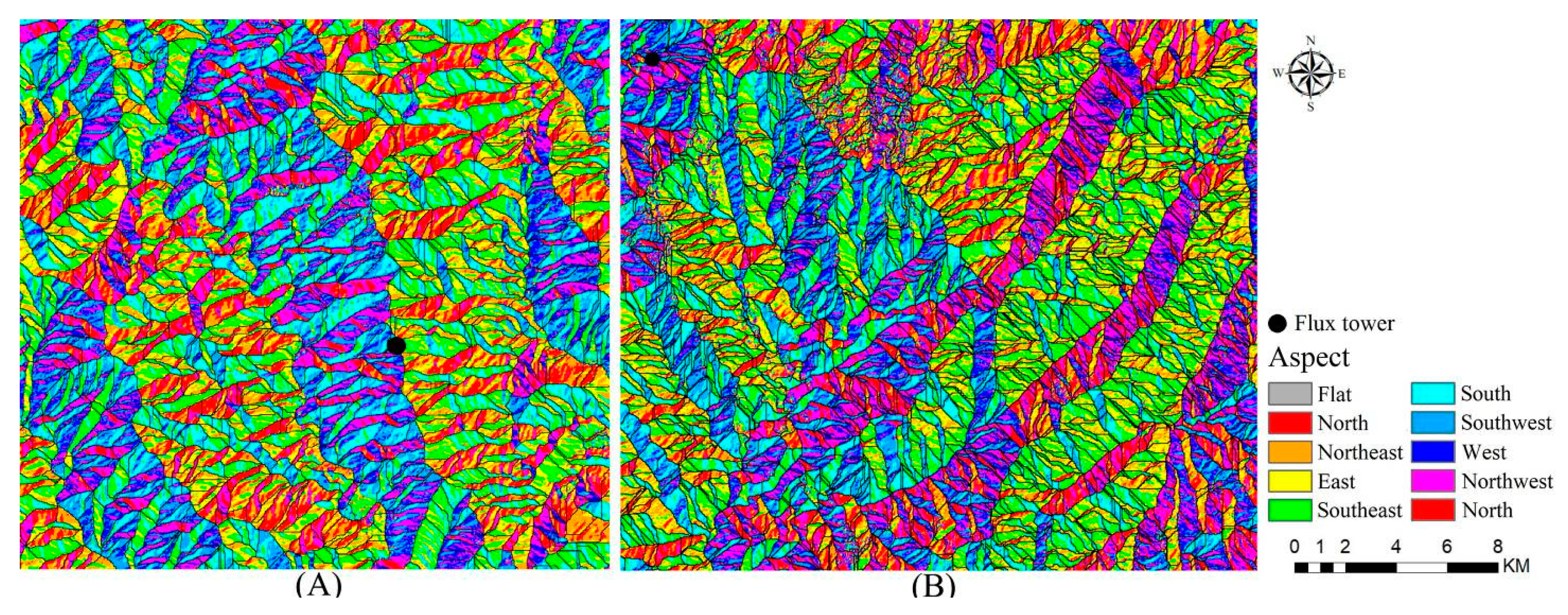
3.1. Results of Slope Unit Delineation

Figure 6 shows the results of the slope unit delineation in the two study areas. The number of slope units in the Huairou and Baotianman study areas are 3196 and 3442, respectively. By overlaying this aspect with the slope unit results, it is clear that the slope-oriented features within the slope units are consistent and in line with the actual situation. The results of the slope units will be used for the subsequent construction of the evapotranspiration disaggregation model based on slope units.

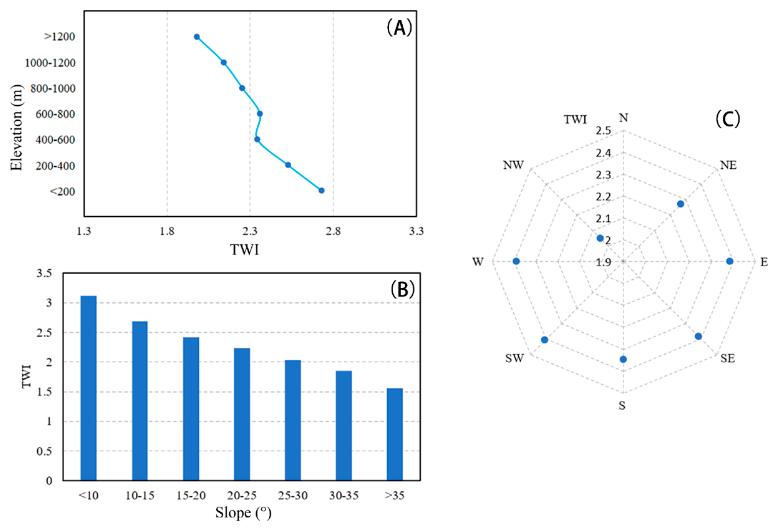
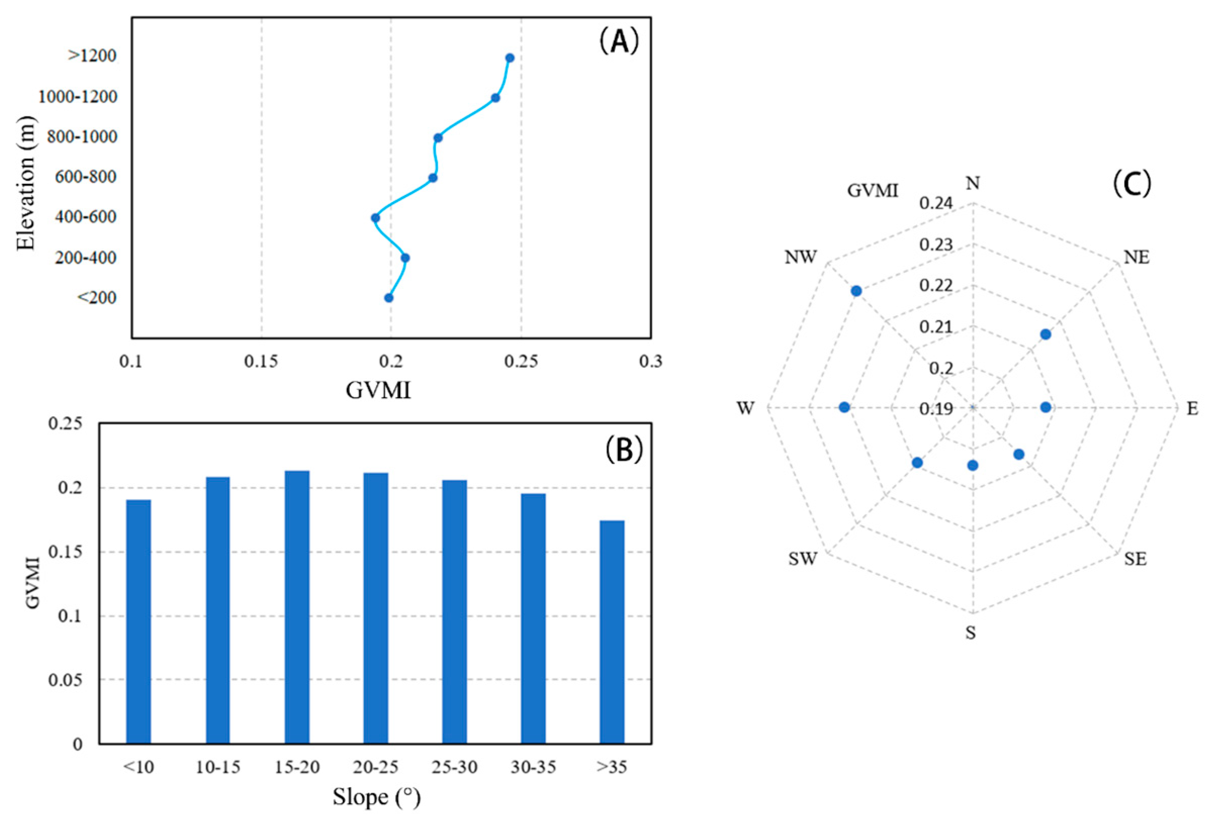
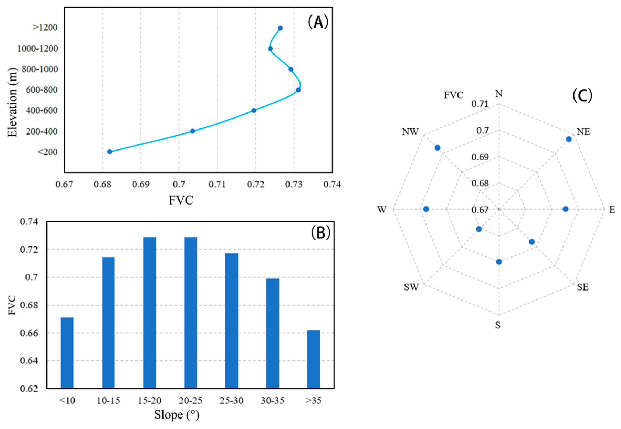
3.2. Factors Reflecting the Differences in Slope-Scale ET

In this section, vegetation cover (FVC), the global vegetation wetness index (GVMI), terrain moisture index (TWI), and net radiation are used to characterize the vegetation factors, moisture factors, and radiation factors that cause inter-slope ET differences, respectively. Here, the annual daily averages of these factor values in the Huairou study area are tabulated based on elevation, slope, and aspect to explore the topographical heterogeneity of these factors.

Figure 7 shows the distribution of net radiation under the conditions of different topographical factors. Due to the influence of topography, the value of Rn is larger at lower elevations and decreases with steeper slopes. For this aspect, the mean value is the largest for the south-facing slope, followed by decreasing values for the southeast, southwest, east, and west-facing slopes, and the smallest value is for the northeast and the northwest-facing slopes. Overall, the south-facing slope has more solar radiation, higher temperatures, and more evapotranspiration, while the north-facing slope has less solar radiation, lower temperatures, and less evapotranspiration.

Figure 8 shows the distribution of the topographical moisture index (TWI) under different topographical factors. The values of the TWI are larger in areas with lower elevation and flatter topography because of the relative direction of water flow, and the tendency of the catchment is larger in lower elevation and flatter areas. The TWI values decrease as the elevation and the slope increase. Regarding this aspect, the average value of the TWI is the smallest for the slopes facing northwest and northeast, and the average value of the TWI is larger for the rest of the slopes.

Figure 9 shows the distribution of the global vegetation wetness index (GVMI) for the conditions of different topographical factors. The GVMI does not vary substantially with elevation and slope. Regarding this aspect, the values of GVMI are the largest for slopes facing west, northwest, and northeast, and the values of GVMI are smaller for the rest of the south-facing and east-facing slopes, which is consistent with the distribution pattern of net radiation. South-facing slopes have more solar radiation, higher temperatures, more ET, and worse vegetation canopy moisture conditions, while north-facing slopes have less solar radiation, lower temperatures, less ET, and better moisture conditions than south-facing slopes.

Figure 10 shows the distribution of fractional vegetation cover (FVC) under different topographical factors. FVC increases to a certain extent as the elevation increases, while FVC is smaller in areas with flatter and steeper slopes, which is related to the characteristics of the study area where there are more mountainous areas, and vegetation grows in higher elevations and steeper slopes. Areas with slopes that are too steep tend to have less vegetation growth. Regarding this aspect, slopes facing northeast and northwest benefit from suitable hydrothermal conditions, and vegetation grows best with larger FVC values, followed by slopes facing east and west, while slopes facing southeast, southwest, and south have smaller FVC values.

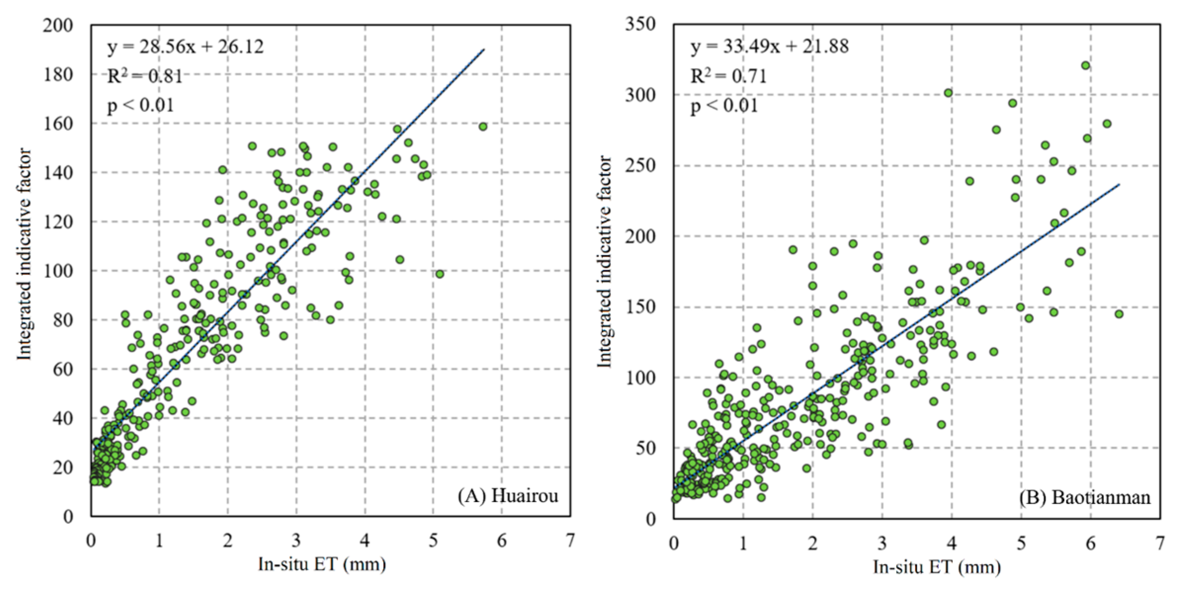
3.3. Results of the Integrated Indicating Factor

An integrated indicating factor reflecting the ET difference in evapotranspiration among the slope units is constructed by further simplifying the P–T equation combining vegetation, moisture, and radiation factors, which is used to disaggregate coarse-resolution ET data. To examine whether the constructed integrated indicating factor can reflect differences in evapotranspiration, validation is carried out in this section using in situ observations of evapotranspiration in the two study areas. Figure 11 shows the time series of the integrated indicating factor compared with the 1 km ETWatch ET and in situ evapotranspiration observations. The trends of the time series match each other and are consistent with the vegetation growth process, where evapotranspiration increases and then decreases throughout the year. The changing process of the integrated indicating factor is relatively flat compared to the 1 km ETWatch ET and in situ evapotranspiration observations, mainly because the integrated indicating factor is hooked into the factors of the FVC and GVMI that are interpolated to a daily time scale. The process of data interpolation makes the changing process of the FVC and GVMI appear flat and then also makes this effect appear for the integrated indicating factor.

Figure 12 shows the scatter plot between the integrated indicating factor and the in situ evapotranspiration observations. It can be clearly seen that the strong correlation between the integrated indicating factor and the in situ evapotranspiration observations indicates that the constructed integrated indicating factor can be utilized to characterize the evapotranspiration variability among slope units. The coefficients of determination (R²) for validation in the study areas of Huairou and Baotianman are both above 0.7. Meanwhile, the integrated indicating factor is strongly correlated with in situ ET in both study areas. Combined with the results of the time series comparison and correlation analysis with scatter plots, the integrated indicating factor is consistent with the trend of ET and correlates well, which can be introduced into the disaggregation method of ET based on slope units.

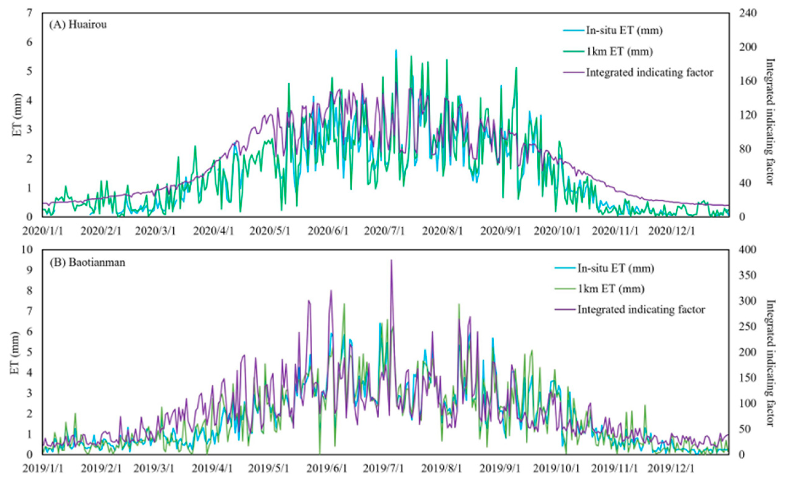
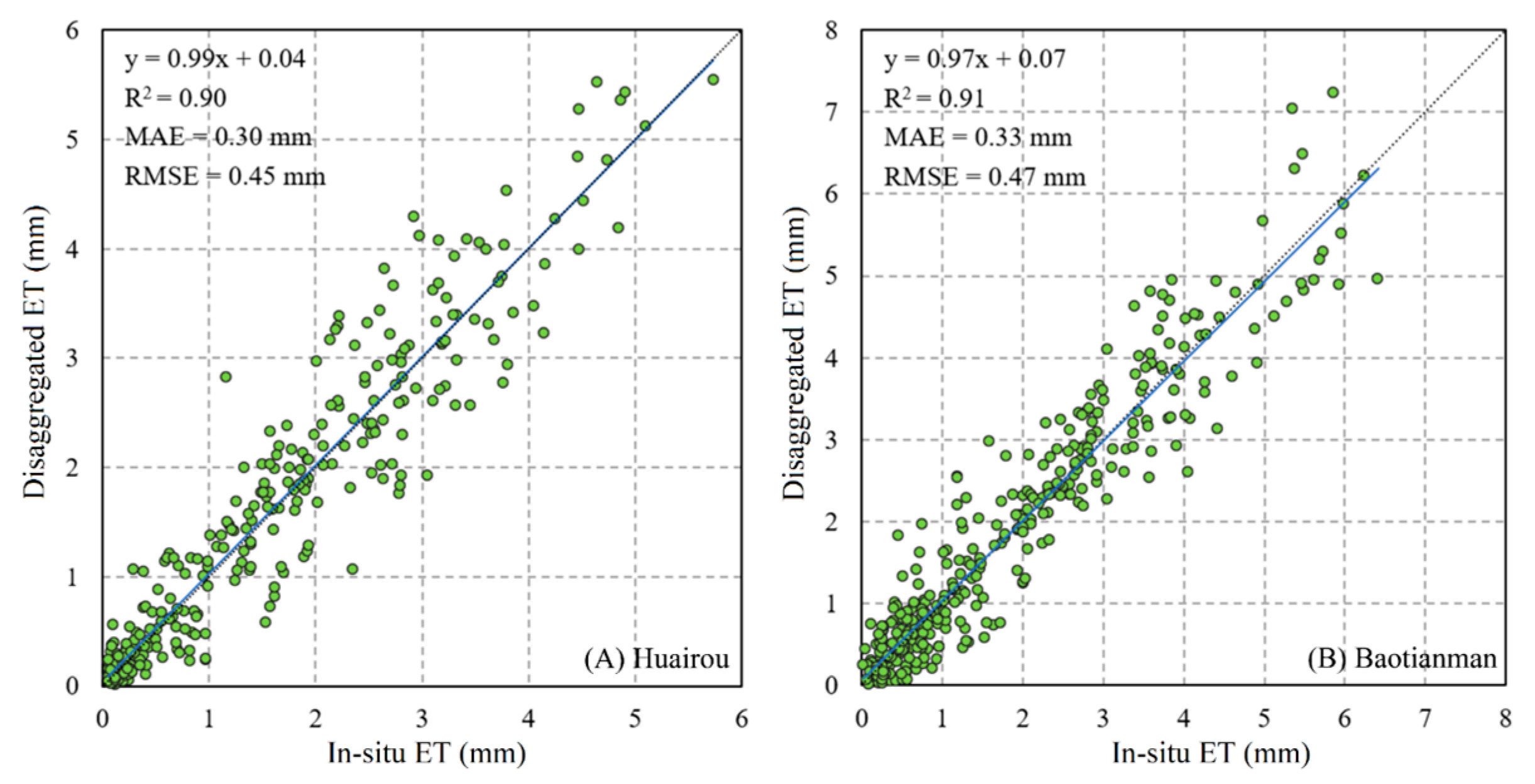
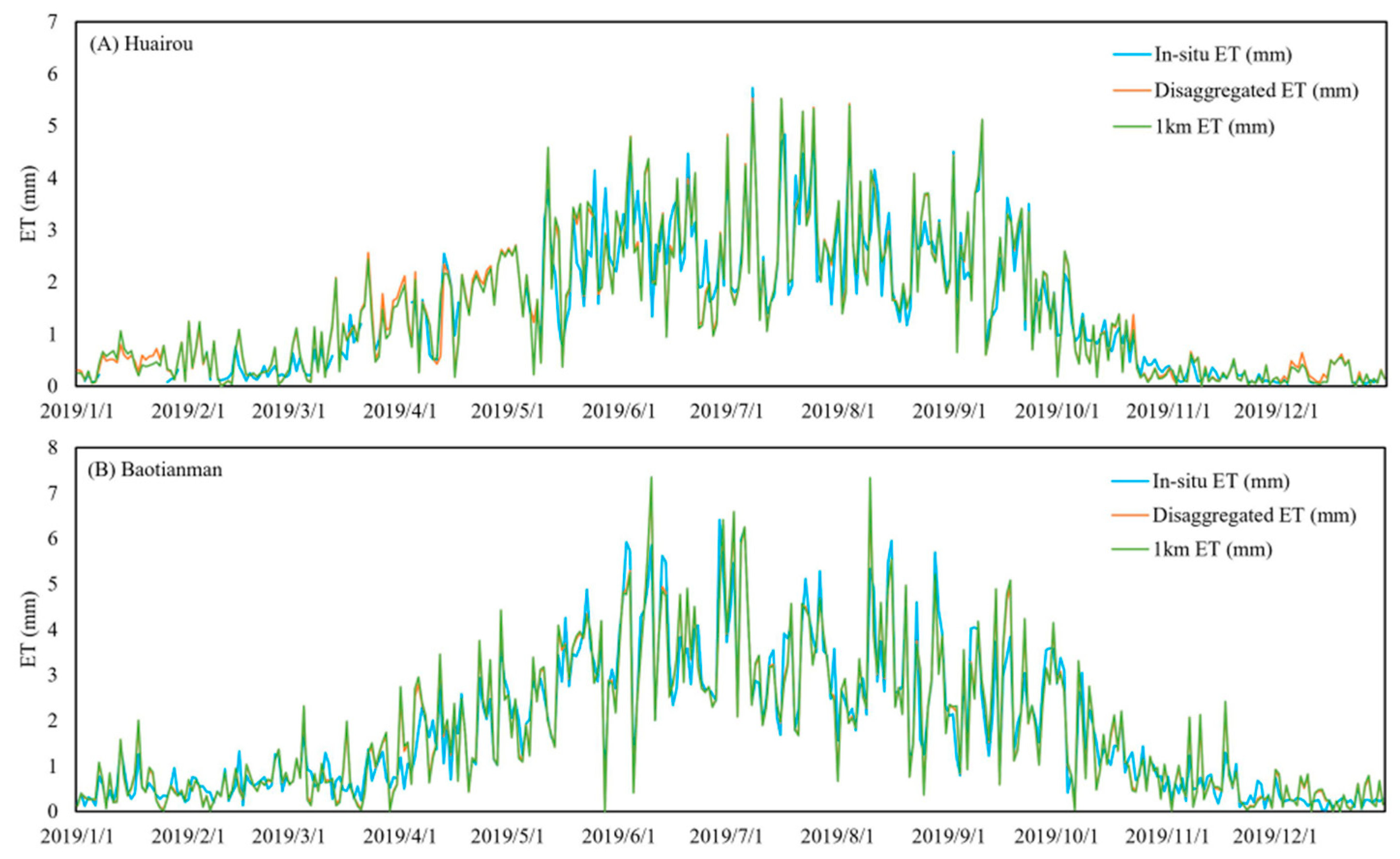
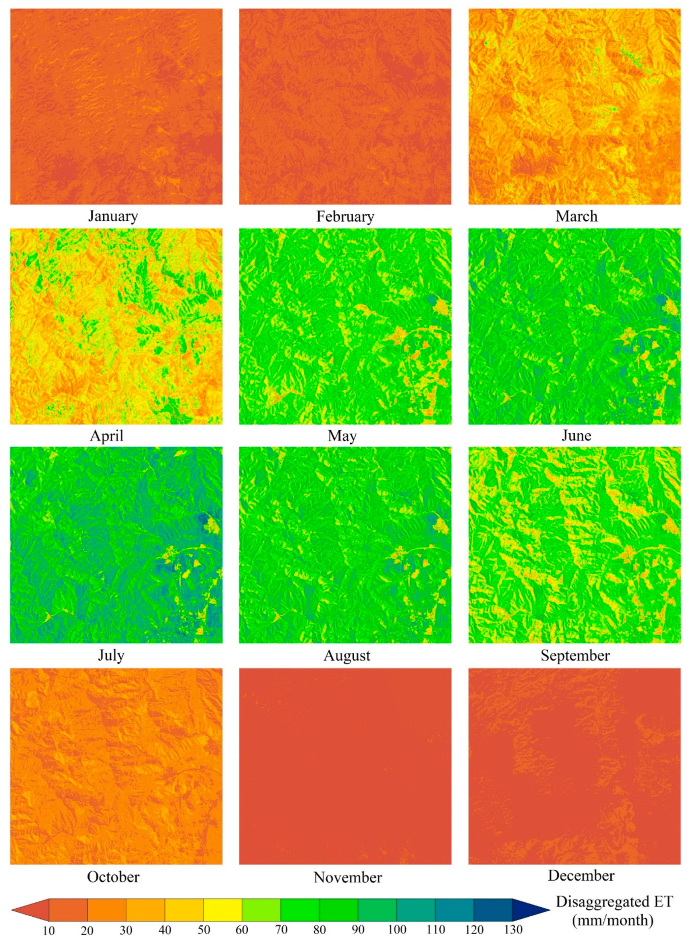
3.4. Results of ET Disaggregation

For the high-spatial-resolution disaggregated ET results, the in situ observations of evapotranspiration are used for validation. Figure 13 shows the validation of disaggregated ET results in Huairou and Baotianman. The coefficients of determination (R²) for disaggregated ET results are 0.9 and 0.91 in Huairou and Baotianman, respectively. The root mean square error (RMSE) values are 0.45 mm and 0.47 mm, respectively, reflecting that the disaggregation model achieves good performance in both study areas. The accuracy of the ETWatch ET data used for input and slope-scale disaggregated ET results are also compared here in two study areas, as shown in

Table 2. Accuracy comparison of the coarse-resolution ETWatch and the disaggregated slope unit-based ET.

	Assessment Indicator	ETWatch ET with 1 km Resolution	Disaggregated Results Based on ETWatch ET
Huairou	R2	0.89	0.90
	RMSE	0.57	0.45
Baotianman	R2	0.89	0.91
	RMSE	0.54	0.47

. In terms of the coefficient of determination (R²), the accuracy of the slope-scale evapotranspiration results for Huairou and Baotianman improved by 0.1 and 0.2, respectively, over the corresponding input coarse-resolution data. Meanwhile, the RMSE decreased by 0.12 mm and 0.07 mm, respectively. The slope-scale ET disaggregation model can achieve further improvement regarding the accuracy of the high-spatial-resolution slope-scale ET on the basis of the accuracy of the input coarse-resolution ET data.

Figure 14 shows the temporal variation process of the high-spatial-resolution disaggregated ET results compared with the in situ evapotranspiration observations. The results show that in both study areas, the variation process of disaggregated ET is very consistent with in situ ET observations. On a day-by-day scale, the disaggregated ET results can adequately reflect the variation in situ evapotranspiration observations. The ET pattern of increasing first and then decreasing throughout the whole year is also consistent with the growth patterns of mountain vegetation in the study area.

Figure 15 and Figure 16 show the month-by-month spatial distribution of slope-scale disaggregated ET results in the Huairou and Baotianman study areas, respectively. The results of the disaggregated ET in both study areas can reflect the characteristics of topographical relief. The underlying surface of the Huairou and Baotianman study areas is mainly forest in mountainous areas, and the change in ET reflects the seasonal change in vegetation growth. From the perspective of monthly differences in evapotranspiration results, Baotianman is located more southward than Huairou; the warming process in spring is earlier than that in Huairou; and vegetation growth also occurs earlier. Additionally, due to the higher net radiation, the evapotranspiration is greater in the primary growing months of vegetation than in Huairou. These characteristics are reflected in the spatial distribution of the monthly disaggregated ET results.

Figure 17 shows the comparison of the spatial distribution of the ETWatch, SSEBop, and FLDAS data and the disaggregated results at a high spatial resolution after applying them to the slope-scale evapotranspiration disaggregation model for the month of August. For the three input ET data, ETWatch and SSEBop are ET data based on the energy balance theory, while FLDAS ET is obtained based on the land surface model (LSM). The spatial resolution of both ETWatch and SSEBop data is 1 km, while the spatial resolution of FLDAS data is only 10 km. As seen in Figure 17, based on the input data with different spatial resolutions and various mechanisms, the slope evapotranspiration disaggregation model can portray an underlying surface with a high spatial resolution using the high-spatial-resolution integrated indicating factor and obtain slope-scale evapotranspiration monitoring results, which show the texture information of terrain distribution to a certain extent. At the same time, the consistency of the slope unit delineation makes both the spatial distribution pattern of the slope-scale evapotranspiration and the disaggregated results of the three input data have some similarity.

Table 3. Accuracy comparison of different coarse-resolution ET data and disaggregated slope unit-based ETs.

	R2	RMSE
ETWatch ET with 1 km resolution	0.89	0.54
Disaggregated results based on ETWatch ET	0.91	0.47
SSEBop ET with 1 km resolution	0.83	0.67
Disaggregated results based on SSEBop ET	0.85	0.58
FLDAS ET with 10 km resolution	0.81	0.62
Disaggregated results based on FLDAS ET	0.82	0.68

shows the accuracy found in the comparison of the three coarse-resolution input data and the corresponding slope-scale evapotranspiration disaggregation results. For the accuracy of slope-scale disaggregated ET results, the coefficients of determination (R²) of ETWatch-, SSEBop-, and FLDAS-based evapotranspiration disaggregation results were improved by 0.02, 0.02, and 0.01, respectively. Except for FLDAS, the ETWatch- and SSEBop-based ET disaggregation results also showed some degree of improvement in RMSE. The validation results show that the slope-scale evapotranspiration disaggregation model developed in this research has good applicability to input data with different mechanisms and spatial resolutions and can achieve a certain degree of improvement in accuracy compared with the input data at a coarse resolution.

4. Discussion

This research proposes a method of ET disaggregation based on slope units, which can fully utilize well-developed coarse-resolution ET data, improve the spatial resolution of ET monitoring, and obtain ET monitoring results reflecting topographical characteristics. The slope unit is a reflection of the topographical similarity, vegetation, and moisture characteristics of the underlying surface, and this monitoring idea based on the slope unit can meet the actual situation of the underlying surface characteristics in mountainous areas. An integrated indicating factor showing evapotranspiration differences among slope units is proposed based on radiation conditions, vegetation landscape, and moisture status, and then the method of ET disaggregation based on slope units is developed with the integrated indicating factor. From the aforementioned disaggregated ET spatial distribution results, it can be seen that the slope-scale ET monitoring results can eliminate the “traces” of coarse-resolution raster boundaries in the traditional downscaling model results and make the model results better reflect the actual situation of evapotranspiration in mountainous areas.

The proposed integrated indicating factor is the theoretical core of this research. Based on the modified P–T formula, which is more mechanistic and has a simpler structure, the integrated indicating factor reflecting the inter-slope evapotranspiration difference is constructed by combining the radiation, vegetation, and moisture factors in a simpler multiplicative manner. The spatial distribution patterns of the inter-slope evapotranspiration influence factors at different elevations, slopes, and aspect ranges reflect the heterogeneity in different topographical conditions, and the integrated indicating factor constructed using these factors can better reflect the differences in evapotranspiration between different slope units within coarse-resolution raster cells. The strong correlation and similar trends of disaggregated ET and in situ observations of ET also add to this conclusion.

As far as the validation results of the evapotranspiration disaggregation model are concerned, this model can achieve more reliable accuracy in mountainous underlying surfaces with complex terrain. From the perspective of spatial distribution, it can also reflect the characteristics of vegetation growth in time and space. The main advantages of the model developed in this chapter are as follows.

First, this study applied ETWatch data to the slope-scale evapotranspiration disaggregation model, and the results show that the model can achieve improved accuracy based on coarse-resolution inputs. The slope-scale evapotranspiration monitoring results are often more accurate and reflective of topographical features.

Second, the principle of the slope-scale evapotranspiration disaggregation model is simple. The model mainly includes two steps: inter-slope evapotranspiration disaggregation and intra-slope evapotranspiration disaggregation. Existing ET models often require complicated model calibration processes and parameterization processes, and the proposed slope-scale model can achieve the large-scale and rapid monitoring of high-spatial-resolution evapotranspiration on the complex underlying surface of the terrain by relying on its simple theoretical basis. Moreover, the model input does not need to consider a specific underlying surface type because the influencing factors of the ET difference among slope units, such as vegetation landscape and moisture conditions, can reflect certain underlying surface characteristics. It is not necessary to use underlying surface-type data as the input, which can avoid the uncertainty introduced by the inaccurate classification of underlying surface types.

In the meantime, the disaggregation model proposed in this research also has some room for development. First, the integrated indicating factor of the inter-slope evapotranspiration difference does not consider the difference in meteorological factors among different slope units caused by topographical factors. The heterogeneity of meteorological factors among slope units is objective. With respect to the sparse distribution of meteorological stations in mountainous areas with complex topography, it is difficult to obtain accurate spatial interpolation results from sparsely distributed meteorological station data. In future research, meteorological parameter data in the existing GLDAS and FLDAS reanalysis datasets need to be combined with meteorological station and topographic data to develop a high-spatial-resolution meteorological dataset that can reflect the topographical heterogeneity of the underlying surface, which can be further introduced into the integrated indicating factor for better simulations of evapotranspiration at the slope scale. In addition, although it is challenging to accurately characterize surface parameters at high spatial resolutions, this model, in its future development, can also strive to improve the representation of key variables such as LST and albedo over complex terrains [86,87,88]. Efforts will be made to incorporate these parameters into the model framework to better capture topographic characteristics.

Moreover, to quantify the magnitude and sources of model uncertainty, it is essential to conduct sensitivity analyses based on the model’s key parameters and driving variables [89,90,91]. Furthermore, more flux data from underlying surfaces in complex terrains should be collected to analyze the contributions of the model’s primary parameters and driving variables to simulate uncertainty across sites with varying elevations, slopes, and aspects. Additionally, the accuracy performance of existing downscaling models under various complex terrain characteristics should be compared to explore the applicability of this model on a broader regional scale [37,92,93].

As far as the delineation of slope units is concerned, the current delineation method is based on high-spatial-resolution digital elevation model data and the principle of hydrology. For topographically complex mountainous regions, the spatial resolution of the digital elevation model (DEM) is ideally as high as possible. Taking into account the cost of monitoring, this study utilized the highest spatial resolution DEM data (12m) currently available for free, which allowed for a relatively accurate division of slope units in the two study areas. As for the threshold of flow accumulation, preliminary tests have indicated that 1000 is the optimal threshold, which can serve as a reference for future research on a similar scale. Although the derived slope units were reasonably distributed, a certain degree of fragmented patches still existed. There was still a gap in the results compared to the actual terrain distribution. In future research, more topographical features, such as plane curvature and profile curvature, can be combined to derive slope units based on the object-oriented segmentation method. The results of the slope units obtained by this type of method are more structured and accurate than the common hydrology-based delineation method, which requires less manual operation [94,95].

5. Conclusions

From a practical perspective, mountainous underlying surfaces are divided into different slope units with high internal homogeneity using a hydrology-based method. The integrated indicating factor is developed to reflect the differences in evapotranspiration among slope units, and the ET data at coarse resolution are disaggregated into different slope units by integrated indicating factors. Then, they are further disaggregated within the slope units to obtain the slope scale ET results at a high spatial resolution. The influencing factors of ET differences among slope units can reflect topographical heterogeneity, while the constructed integrated indicating factor is strongly correlated with the in situ ET observation data. The coefficients of determination (R²) for model validation reach 0.9 and 0.91 for coarse-resolution ET-based disaggregation results, and the root mean square errors are 0.45 mm and 0.47 mm in Huairou and Baotianman, respectively. The temporal trends of the slope-scale evapotranspiration disaggregation results and the ground observations are also in good agreement, indicating that the slope-scale evapotranspiration disaggregation model in this study achieved good performances in both study areas. Compared with the input ETWatch ET data with a 1 km spatial resolution, the accuracy of disaggregated ET results in both study areas improved compared to the input data. The coefficients of determination (R²) in Huairou and Baotianman improved by 0.01 and 0.02, respectively, and the root mean square errors decreased by 0.12 mm and 0.07 mm, respectively. The model results can not only reflect the evapotranspiration heterogeneity at the slope scale within coarse-resolution raster cells but can also improve accuracy compared with input data. The ET disaggregation model based on the slope unit breaks through the traditional downscaling method of taking coarse-resolution raster cells as the basic unit and utilizes slope units for the disaggregation process, which is more in line with the actual topographical relief in mountainous areas. High-spatial-resolution evapotranspiration monitoring results at the slope scale are obtained based on the developed integrated indicating factor. The model has strong application prospects in mountain water resource management.

References

1. Funnell, D.C.; Price, M.F. Mountain geography: A review. Geogr. J. 2003, 169, 183–190. [Google Scholar] [CrossRef]
2. Ives, J.D.; Messerli, B. The Himalayan Dilemma: Reconciling Development and Conservation; Routledge: London, UK, 2003. [Google Scholar]
3. Gaertner, B.A.; Zegre, N.; Warner, T.; Fernandez, R.; He, Y.; Merriam, E.R. Climate, forest growing season, and evapotranspiration changes in the central Appalachian Mountains, USA. Sci. Total Environ. 2019, 650, 1371–1381. [Google Scholar] [CrossRef] [PubMed]
4. Grêt-Regamey, A.; Brunner, S.H.; Kienast, F. Mountain ecosystem services: Who cares? Mt. Res. Dev. 2012, 32. [Google Scholar] [CrossRef]
5. Briner, S.; Huber, R.; Bebi, P.; Elkin, C.; Schmatz, D.R.; Grêt-Regamey, A. Trade-offs between ecosystem services in a mountain region. Ecol. Soc. 2013, 18, 35. [Google Scholar] [CrossRef]
6. Gret-Regamey, A.; Weibel, B. Global assessment of mountain ecosystem services using earth observation data. Ecosyst. Serv. 2020, 46, 101213. [Google Scholar] [CrossRef]
7. Jasechko, S.; Sharp, Z.D.; Gibson, J.J.; Birks, S.J.; Yi, Y.; Fawcett, P.J. Terrestrial water fluxes dominated by transpiration. Nature 2013, 496, 347–350. [Google Scholar] [CrossRef]
8. Vinukollu, R.; Sheffield, J.; Ferguson, C.; Pan, M.; Wood, E. Developing Evapotranspiration Data Records for the Global Terrestrial Water Cycle. In Proceedings of the AGU Fall Meeting Abstracts, San Francisco, CA, USA, 14–18 December 2009; p. N43C-1159. [Google Scholar]
9. Elnashar, A.; Shojaeezadeh, S.A.; Weber, T.K.D. A Multi-Model approach for remote Sensing-Based actual evapotranspiration mapping using Google Earth Engine (ETMapper-GEE). J. Hydrol. 2025, 657, 133062. [Google Scholar] [CrossRef]
10. Ma, Z.; Yan, N.; Wu, B.; Stein, A.; Zhu, W.; Zeng, H. Variation in actual evapotranspiration following changes in climate and vegetation cover during an ecological restoration period (2000–2015) in the Loess Plateau, China. Sci. Total Environ. 2019, 689, 534–545. [Google Scholar] [CrossRef]
11. Elnashar, A.; Zeng, H.; Wu, B.; Gebremicael, T.G.; Marie, K. Assessment of environmentally sensitive areas to desertification in the Blue Nile Basin driven by the MEDALUS-GEE framework. Sci. Total Environ. 2022, 815, 152925. [Google Scholar] [CrossRef]
12. Zeng, H.; Elnashar, A.; Wu, B.; Zhang, M.; Zhu, W.; Tian, F.; Ma, Z. A framework for separating natural and anthropogenic contributions to evapotranspiration of human-managed land covers in watersheds based on machine learning. Sci. Total Environ. 2022, 823, 153726. [Google Scholar] [CrossRef]
13. Nagler, P.L.; Glenn, E.P.; Hinojosa-Huerta, O. Synthesis of ground and remote sensing data for monitoring ecosystem functions in the Colorado River Delta, Mexico. Remote Sens. Environ. 2009, 113, 1473–1485. [Google Scholar]
14. Peng, H.; Jia, Y.; Zhan, C.; Xu, W. Topographic controls on ecosystem evapotranspiration and net primary productivity under climate warming in the Taihang Mountains, China. J. Hydrol. 2020, 581, 124394. [Google Scholar]
15. Ma, Z.; Wu, B.; Yan, N.; Zhu, W.; Xu, J. Coupling water and carbon processes to estimate field-scale maize evapotranspiration with Sentinel-2 data. Agric. For. Meteorol. 2021, 306, 108421. [Google Scholar]
16. Elnashar, A.; Wang, L.; Wu, B.; Zhu, W.; Zeng, H. Synthesis of global actual evapotranspiration from 1982 to 2019. Earth Syst. Sci. Data 2021, 13, 447–480. [Google Scholar] [CrossRef]
17. Vinukollu, R.K.; Wood, E.F.; Ferguson, C.R.; Fisher, J.B. Global estimates of evapotranspiration for climate studies using multi-sensor remote sensing data: Evaluation of three process-based approaches. Remote Sens. Environ. 2011, 115, 801–823. [Google Scholar]
18. Wang, L.; Wu, B.; Elnashar, A.; Zeng, H.; Zhu, W.; Yan, N. Synthesizing a regional territorial evapotranspiration dataset for Northern China. Remote Sens. 2021, 13, 1076. [Google Scholar] [CrossRef]
19. Dile, Y.T.; Ayana, E.K.; Worqlul, A.W.; Xie, H.; Srinivasan, R.; Lefore, N.; You, L.; Clarke, N. Evaluating satellite-based evapotranspiration estimates for hydrological applications in data-scarce regions: A case in Ethiopia. Sci. Total Environ. 2020, 743, 140702. [Google Scholar]
20. Wang, L.; Wu, B.; Elnashar, A.; Zhu, W.; Yan, N.; Ma, Z.; Liu, S.; Niu, X. Incorporation of net radiation model considering complex terrain in evapotranspiration determination with Sentinel-2 data. Remote Sens. 2022, 14, 1191. [Google Scholar] [CrossRef]
21. Abiodun, O.O.; Guan, H.; Post, V.E.; Batelaan, O. Comparison of MODIS and SWAT evapotranspiration over a complex terrain at different spatial scales. Hydrol. Earth Syst. Sci. 2018, 22, 2775–2794. [Google Scholar] [CrossRef]
22. Yang, Y.; Chen, R.; Song, Y.; Han, C.; Liu, J.; Liu, Z. Sensitivity of potential evapotranspiration to meteorological factors and their elevational gradients in the Qilian Mountains, northwestern China. J. Hydrol. 2019, 568, 147–159. [Google Scholar]
23. Cristóbal, J.; Poyatos, R.; Ninyerola, M.; Llorens, P.; Pons, X. Combining remote sensing and GIS climate modelling to estimate daily forest evapotranspiration in a Mediterranean mountain area. Hydrol. Earth Syst. Sci. 2011, 15, 1563–1575. [Google Scholar]
24. Minderlein, S.; Menzel, L. Evapotranspiration and energy balance dynamics of a semi-arid mountainous steppe and shrubland site in Northern Mongolia. Environ. Earth Sci. 2015, 73, 593–609. [Google Scholar] [CrossRef]
25. Atchley, A.L.; Maxwell, R.M. Influences of subsurface heterogeneity and vegetation cover on soil moisture, surface temperature and evapotranspiration at hillslope scales. Hydrogeol. J. 2011, 19, 289. [Google Scholar]
26. Chen, X.; Su, Z.; Ma, Y.; Yang, K.; Wang, B. Estimation of surface energy fluxes under complex terrain of Mt. Qomolangma over the Tibetan Plateau. Hydrol. Earth Syst. Sci. 2013, 17, 1607–1618. [Google Scholar]
27. Liu, X.; Shen, Y.; Li, H.; Guo, Y.; Pei, H.; Dong, W. Estimation of land surface evapotranspiration over complex terrain based on multi-spectral remote sensing data. Hydrol. Process. 2017, 31, 446–461. [Google Scholar] [CrossRef]
28. Zhao, X.; Liu, Y. Relative contribution of the topographic influence on the triangle approach for evapotranspiration estimation over mountainous areas. Adv. Meteorol. 2014, 2014, 584040. [Google Scholar]
29. Lima, R.N.d.S.; Ribeiro, C.B.d.M. Spatial variability of daily evapotranspiration in a mountainous watershed by coupling surface energy balance and solar radiation model with gridded weather dataset. In Proceedings of the 2nd International Electronic Conference on Remote Sensing, Online, 22 March–5 April 2018; p. 342. [Google Scholar]
30. Wang, D.; Zhan, Y.; Yu, T.; Liu, Y.; Jin, X.; Ren, X.; Chen, X.; Liu, Q. Improving meteorological input for surface energy balance system utilizing mesoscale weather research and forecasting model for estimating daily actual evapotranspiration. Water 2019, 12, 9. [Google Scholar] [CrossRef]
31. Cherif, I.; Alexandridis, T.; Jauch, E.; Chambel-Leitao, P.; Almeida, C. Improving remotely sensed actual evapotranspiration estimation with raster meteorological data. Int. J. Remote Sens. 2015, 36, 4606–4620. [Google Scholar]
32. Qian, Q.; Wu, B.; Xiong, J. Interpolation system for generating meteorological surfaces using to compute evapotranspiration in Haihe River Basin. In Proceedings of the 2005 IEEE International Geoscience and Remote Sensing Symposium, Seoul, Republic of Korea, 25–29 July 2005; IGARSS’05; p. 4. [Google Scholar]
33. Goulden, M.; Anderson, R.; Bales, R.; Kelly, A.; Meadows, M.; Winston, G. Evapotranspiration along an elevation gradient in California’s Sierra Nevada. J. Geophys. Res. Biogeosci. 2012, 117. [Google Scholar] [CrossRef]
34. Li, S.; Tarboton, D.G.; McKee, M. GIS-Based Temperature Interpolation for Distributed Modelling of Reference Evapotranspiration. 2003. Available online: https://digitalcommons.usu.edu/cee_facpub/2218/ (accessed on 16 January 2025).
35. Allen, R.G.; Tasumi, M.; Trezza, R. Satellite-based energy balance for mapping evapotranspiration with internalized calibration (METRIC)—Model. J. Irrig. Drain. Eng. 2007, 133, 380–394. [Google Scholar] [CrossRef]
36. Sun, R.; Zhang, B. Topographic effects on spatial pattern of surface air temperature in complex mountain environment. Environ. Earth Sci. 2016, 75, 1–12. [Google Scholar] [CrossRef]
37. Mahour, M.; Tolpekin, V.; Stein, A.; Sharifi, A. A comparison of two downscaling procedures to increase the spatial resolution of mapping actual evapotranspiration. Isprs J. Photogramm. Remote Sens. 2017, 126, 56–67. [Google Scholar] [CrossRef]
38. Shen, T.; Wu, B.; Yan, N.; Zhu, W. An NDVI-Based Statistical ET Downscaling Method. Water 2017, 9, 995. [Google Scholar] [CrossRef]
39. Jiang, C.; Guan, K.; Pan, M.; Ryu, Y.; Wang, S. BESS-STAIR: A framework to estimate daily, 30-meter, and allweather crop evapotranspiration using multi-source satellite data for the U.S. Corn Belt. Hydrol. Earth Syst. Sci. Discuss. 2019, 1–36. [Google Scholar] [CrossRef]
40. Tan, S.; Wu, B.; Yan, N. A method for downscaling daily evapotranspiration based on 30-m surface resistance. J. Hydrol. 2019, 577, 123882. [Google Scholar] [CrossRef]
41. Carrara, A. Drainage and divide networks derived from high-fidelity digital terrain models. In Quantitative Analysis of Mineral and Energy Resources; Springer: Berlin/Heidelberg, Germany, 1988; pp. 581–597. [Google Scholar]
42. Guzzetti, F.; Carrara, A.; Cardinali, M.; Reichenbach, P. Landslide hazard evaluation: A review of current techniques and their application in a multi-scale study, Central Italy. Geomorphology 1999, 31, 181–216. [Google Scholar] [CrossRef]
43. Xie, M.; Esaki, T.; Zhou, G. GIS-based probabilistic mapping of landslide hazard using a three-dimensional deterministic model. Nat. Hazards 2004, 33, 265–282. [Google Scholar] [CrossRef]
44. Holland, P.; Steyn, D. Vegetational responses to latitudinal variations in slope angle and aspect. J. Biogeogr. 1975, 2, 179–183. [Google Scholar] [CrossRef]
45. Chen, J.M.; Black, T. Defining leaf area index for non-flat leaves. Plant Cell Environ. 1992, 15, 421–429. [Google Scholar] [CrossRef]
46. Wang, K.; Liang, S. An improved method for estimating global evapotranspiration based on satellite determination of surface net radiation, vegetation index, temperature, and soil moisture. J. Hydrometeorol. 2008, 9, 712–727. [Google Scholar] [CrossRef]
47. Zha, T.; Barr, A.G.; van der Kamp, G.; Black, T.A.; McCaughey, J.H.; Flanagan, L.B. Interannual variation of evapotranspiration from forest and grassland ecosystems in western Canada in relation to drought. Agric. For. Meteorol. 2010, 150, 1476–1484. [Google Scholar]
48. Metzen, D.; Sheridan, G.J.; Benyon, R.G.; Bolstad, P.V.; Griebel, A.; Lane, P.N. Spatio-temporal transpiration patterns reflect vegetation structure in complex upland terrain. Sci. Total Environ. 2019, 694, 133551. [Google Scholar] [CrossRef]
49. Ward, A.D.; Trimble, S.W. Environmental Hydrology; CRC Press: Boca Raton, FL, USA, 2003. [Google Scholar]
50. Williams, C.; McNamara, J.; Chandler, D. Controls on the temporal and spatial variability of soil moisture in a mountainous landscape: The signature of snow and complex terrain. Hydrol. Earth Syst. Sci. 2009, 13, 1325–1336. [Google Scholar]
51. Cao, B.; Yu, L.; Naipal, V.; Ciais, P.; Li, W.; Zhao, Y.; Wei, W.; Chen, D.; Liu, Z.; Gong, P. A 30 m terrace mapping in China using Landsat 8 imagery and digital elevation model based on the Google Earth Engine. Earth Syst. Sci. Data 2021, 13, 2437–2456. [Google Scholar]
52. Farwell, L.S.; Gudex-Cross, D.; Anise, I.E.; Bosch, M.J.; Olah, A.M.; Radeloff, V.C.; Razenkova, E.; Rogova, N.; Silveira, E.M.; Smith, M.M. Satellite image texture captures vegetation heterogeneity and explains patterns of bird richness. Remote Sens. Environ. 2021, 253, 112175. [Google Scholar]
53. Vrieling, A.; Meroni, M.; Darvishzadeh, R.; Skidmore, A.K.; Wang, T.; Zurita-Milla, R.; Oosterbeek, K.; O’Connor, B.; Paganini, M. Vegetation phenology from Sentinel-2 and field cameras for a Dutch barrier island. Remote Sens. Environ. 2018, 215, 517–529. [Google Scholar] [CrossRef]
54. Sun, Y.; Qin, Q.; Ren, H.; Zhang, T.; Chen, S. Red-edge band vegetation indices for leaf area index estimation from Sentinel-2/MSI imagery. IEEE Trans. Geosci. Remote Sens. 2019, 58, 826–840. [Google Scholar]
55. Akbar, M.; Arisanto, P.; Sukirno, B.; Merdeka, P.; Priadhi, M.; Zallesa, S. Mangrove vegetation health index analysis by implementing NDVI (normalized difference vegetation index) classification method on sentinel-2 image data case study: Segara Anakan, Kabupaten Cilacap. IOP Conf. Ser. Earth Environ. Sci. 2020, 584, 012069. [Google Scholar] [CrossRef]
56. Rujoiu-Mare, M.-R.; Olariu, B.; Mihai, B.-A.; Nistor, C.; Săvulescu, I. Land cover classification in Romanian Carpathians and Subcarpathians using multi-date Sentinel-2 remote sensing imagery. Eur. J. Remote Sens. 2017, 50, 496–508. [Google Scholar]
57. Gašparović, M.; Jogun, T. The effect of fusing Sentinel-2 bands on land-cover classification. Int. J. Remote Sens. 2018, 39, 822–841. [Google Scholar] [CrossRef]
58. Phiri, D.; Simwanda, M.; Salekin, S.; Nyirenda, V.R.; Murayama, Y.; Ranagalage, M. Sentinel-2 data for land cover/use mapping: A review. Remote Sens. 2020, 12, 2291. [Google Scholar] [CrossRef]
59. Saleem, A.; Awange, J. Coastline shift analysis in data deficient regions: Exploiting the high spatio-temporal resolution Sentinel-2 products. Catena 2019, 179, 6–19. [Google Scholar]
60. Li, J.; Peng, B.; Wei, Y.; Ye, H. Accurate extraction of surface water in complex environment based on Google Earth Engine and Sentinel-2. PLoS ONE 2021, 16, e0253209. [Google Scholar] [CrossRef]
61. Puletti, N.; Mattioli, W.; Bussotti, F.; Pollastrini, M. Monitoring the effects of extreme drought events on forest health by Sentinel-2 imagery. J. Appl. Remote Sens. 2019, 13, 020501. [Google Scholar]
62. Haghighian, F.; Yousefi, S.; Keesstra, S. Identifying tree health using sentinel-2 images: A case study on Tortrix viridana L. infected oak trees in Western Iran. Geocarto Int. 2022, 37, 304–314. [Google Scholar]
63. Wu, B.; Liu, S.; Zhu, W.; Yu, M.; Yan, N.; Xing, Q. A method to estimate sunshine duration using cloud classification data from a geostationary meteorological satellite (FY-2D) over the Heihe River Basin. Sensors 2016, 16, 1859. [Google Scholar] [CrossRef]
64. Rossi, C.; Gonzalez, F.R.; Fritz, T.; Yague-Martinez, N.; Eineder, M. TanDEM-X calibrated raw DEM generation. ISPRS J. Photogramm. Remote Sens. 2012, 73, 12–20. [Google Scholar]
65. Kljun, N.; Calanca, P.; Rotach, M.; Schmid, H.P. A simple two-dimensional parameterisation for Flux Footprint Prediction (FFP). Geosci. Model Dev. 2015, 8, 3695–3713. [Google Scholar]
66. Babel, W.; Charuchittipan, D.; Zhao, P.; Biermann, T.; Gatzsche, K.; Foken, T. Application of an energy balance correction method for turbulent flux measurements based on buoyancy. In Proceedings of the EGU General Assembly Conference Abstracts, Vienna, Austria, 27 April–2 May 2014; p. 6936. [Google Scholar]
67. Liu, S.; Xu, Z.; Zhu, Z.; Jia, Z.; Zhu, M. Measurements of evapotranspiration from eddy-covariance systems and large aperture scintillometers in the Hai River Basin, China. J. Hydrol. 2013, 487, 24–38. [Google Scholar]
68. Wu, B.; Zhu, W.; Yan, N.; Xing, Q.; Wang, L. Regional Actual Evapotranspiration Estimation with Land and Meteorological Variables Derived from Multi-Source Satellite Data. Remote Sens. 2020, 12, 332. [Google Scholar] [CrossRef]
69. Dodson, R.; Marks, D. Daily air temperature interpolated at high spatial resolution over a large mountainous region. Clim. Res. 1997, 8, 1–20. [Google Scholar] [CrossRef]
70. Wu, B.; Yan, N.; Xiong, J.; Bastiaanssen, W.; Zhu, W.; Stein, A. Validation of ETWatch using field measurements at diverse landscapes: A case study in Hai Basin of China. J. Hydrol. 2012, 436, 67–80. [Google Scholar] [CrossRef]
71. Tan, S.; Wu, B.; Yan, N.; Zeng, H. Satellite-based water consumption dynamics monitoring in an extremely arid area. Remote Sens. 2018, 10, 1399. [Google Scholar] [CrossRef]
72. Cleugh, H.A.; Leuning, R.; Mu, Q.; Running, S.W. Regional evaporation estimates from flux tower and MODIS satellite data. Remote Sens. Environ. 2007, 106, 285–304. [Google Scholar]
73. Mu, Q.; Heinsch, F.A.; Zhao, M.; Running, S.W. Development of a global evapotranspiration algorithm based on MODIS and global meteorology data. Remote Sens. Environ. 2007, 111, 519–536. [Google Scholar]
74. Leuning, R.; Zhang, Y.; Rajaud, A.; Cleugh, H.; Tu, K. A simple surface conductance model to estimate regional evaporation using MODIS leaf area index and the Penman-Monteith equation. Water Resour. Res. 2008, 44. [Google Scholar] [CrossRef]
75. Mu, Q.; Zhao, M.; Running, S.W. Improvements to a MODIS global terrestrial evapotranspiration algorithm. Remote Sens. Environ. 2011, 115, 1781–1800. [Google Scholar] [CrossRef]
76. Fisher, J.B.; Tu, K.P.; Baldocchi, D.D. Global estimates of the land–atmosphere water flux based on monthly AVHRR and ISLSCP-II data, validated at 16 FLUXNET sites. Remote Sens. Environ. 2008, 112, 901–919. [Google Scholar]
77. Yao, Y.; Liang, S.; Cheng, J.; Liu, S.; Fisher, J.B.; Zhang, X.; Jia, K.; Zhao, X.; Qin, Q.; Zhao, B. MODIS-driven estimation of terrestrial latent heat flux in China based on a modified Priestley–Taylor algorithm. Agric. For. Meteorol. 2013, 171, 187–202. [Google Scholar] [CrossRef]
78. Ceccato, P.; Flasse, S.; Gregoire, J.-M. Designing a spectral index to estimate vegetation water content from remote sensing data: Part 2. Validation and applications. Remote Sens. Environ. 2002, 82, 198–207. [Google Scholar] [CrossRef]
79. Ceccato, P.; Gobron, N.; Flasse, S.; Pinty, B.; Tarantola, S. Designing a spectral index to estimate vegetation water content from remote sensing data: Part 1: Theoretical approach. Remote Sens. Environ. 2002, 82, 188–197. [Google Scholar]
80. Cao, R.; Chen, Y.; Shen, M.; Chen, J.; Zhou, J.; Wang, C.; Yang, W. A simple method to improve the quality of NDVI time-series data by integrating spatiotemporal information with the Savitzky-Golay filter. Remote Sens. Environ. 2018, 217, 244–257. [Google Scholar]
81. Shwetha, H.R.; Nagesh Kumar, D. Estimation of daily vegetation coefficients using MODIS data for clear and cloudy sky conditions. Int. J. Remote Sens. 2018, 39, 3776–3800. [Google Scholar]
82. Western, A.W.; Grayson, R.B.; Blöschl, G.; Willgoose, G.R.; McMahon, T.A. Observed spatial organization of soil moisture and its relation to terrain indices. Water Resour. Res. 1999, 35, 797–810. [Google Scholar]
83. Kopecký, M.; Macek, M.; Wild, J. Topographic Wetness Index calculation guidelines based on measured soil moisture and plant species composition. Sci. Total Environ. 2021, 757, 143785. [Google Scholar] [CrossRef]
84. Senay, G.B.; Bohms, S.; Singh, R.K.; Gowda, P.H.; Velpuri, N.M.; Alemu, H.; Verdin, J.P. Operational evapotranspiration mapping using remote sensing and weather datasets: A new parameterization for the SSEB approach. JAWRA J. Am. Water Resour. Assoc. 2013, 49, 577–591. [Google Scholar] [CrossRef]
85. McNally, A.; Arsenault, K.; Kumar, S.; Shukla, S.; Peterson, P.; Wang, S.; Funk, C.; Peters-Lidard, C.D.; Verdin, J.P. A land data assimilation system for sub-Saharan Africa food and water security applications. Sci. Data 2017, 4, 1–19. [Google Scholar]
86. Yang, X.; Zuo, X.; Xie, W.; Li, Y.; Guo, S.; Zhang, H. A correction method of NDVI topographic shadow effect for rugged terrain. IEEE J. Sel. Top. Appl. Earth Obs. Remote Sens. 2022, 15, 8456–8472. [Google Scholar] [CrossRef]
87. Mutiibwa, D.; Strachan, S.; Albright, T. Land surface temperature and surface air temperature in complex terrain. IEEE J. Sel. Top. Appl. Earth Obs. Remote Sens. 2015, 8, 4762–4774. [Google Scholar]
88. Wen, J.; Zhao, X.; Liu, Q.; Tang, Y.; Dou, B. An improved land-surface albedo algorithm with DEM in rugged terrain. IEEE Geosci. Remote Sens. Lett. 2013, 11, 883–887. [Google Scholar]
89. Tran, B.N.; Van Der Kwast, J.; Seyoum, S.; Uijlenhoet, R.; Jewitt, G.; Mul, M. Uncertainty assessment of satellite remote-sensing-based evapotranspiration estimates: A systematic review of methods and gaps. Hydrol. Earth Syst. Sci. 2023, 27, 4505–4528. [Google Scholar] [CrossRef]
90. Badgley, G.; Fisher, J.B.; Jiménez, C.; Tu, K.P.; Vinukollu, R. On uncertainty in global terrestrial evapotranspiration estimates from choice of input forcing datasets. J. Hydrometeorol. 2015, 16, 1449–1455. [Google Scholar] [CrossRef]
91. Long, D.; Longuevergne, L.; Scanlon, B.R. Uncertainty in evapotranspiration from land surface modeling, remote sensing, and GRACE satellites. Water Resour. Res. 2014, 50, 1131–1151. [Google Scholar] [CrossRef]
92. Yang, Z.; Pan, X.; Liu, Y.; Tansey, K.; Yuan, J.; Wang, Z.; Liu, S.; Yang, Y. Evaluation of spatial downscaling for satellite retrieval of evapotranspiration from the nonparametric approach in an arid area. J. Hydrol. 2024, 628, 130538. [Google Scholar]
93. Bisquert, M.; Sánchez, J.; López-Urrea, R.; Caselles, V. Estimating high resolution evapotranspiration from disaggregated thermal images. Remote Sens. Environ. 2016, 187, 423–433. [Google Scholar] [CrossRef]
94. Drăguţ, L.; Blaschke, T. Automated classification of landform elements using object-based image analysis. Geomorphology 2006, 81, 330–344. [Google Scholar]
95. Youssef, A.M. Landslide susceptibility delineation in the Ar-Rayth area, Jizan, Kingdom of Saudi Arabia, using analytical hierarchy process, frequency ratio, and logistic regression models. Environ. Earth Sci. 2015, 73, 8499–8518. [Google Scholar]
Figure 1. Study area.
Remotesensing 17 01201 g001
Figure 2. Footprint area of EC observations in Huairou and Baotianman.
Remotesensing 17 01201 g002
Figure 3. Flow chart illustrating the process of ETWatch data disaggregated to slope units.
Remotesensing 17 01201 g003
Figure 4. Flow chart illustrating the delineation of slope units.
Remotesensing 17 01201 g004
Figure 5. Flow chart for slope unit-based ET disaggregation scheme.
Remotesensing 17 01201 g005
Figure 6. Delineated slope units of the two study areas: (A) Huairou and (B) Baotianman.
Remotesensing 17 01201 g006
Figure 7. Net radiation distribution in different terrain conditions: (A) elevation, (B) slope, and (C) aspect.
Remotesensing 17 01201 g007
Figure 8. TWI distribution in different terrain conditions: (A) elevation, (B) slope, and (C) aspect.
Remotesensing 17 01201 g008
Figure 9. GVMI distribution in different terrain conditions: (A) elevation, (B) slope, and (C) aspect.
Remotesensing 17 01201 g009
Figure 10. FVC distribution in different terrain conditions: (A) elevation, (B) slope, and (C) aspect.
Remotesensing 17 01201 g010
Figure 11. Time series of integrated indicating factors: 1 km ET and in situ ET.
Remotesensing 17 01201 g011
Figure 12. Scatter plot of the integrated indicating factor and in situ ET.
Remotesensing 17 01201 g012
Figure 13. Scatter plot of the disaggregated slope unit-based ET and the in situ ET.
Remotesensing 17 01201 g013
Figure 14. Time series of the disaggregated slope unit-based ET and the in situ ET.
Remotesensing 17 01201 g014
Figure 15. Monthly spatial distribution of the disaggregated slope unit-based ET in Huairou.
Remotesensing 17 01201 g015
Figure 16. Monthly spatial distribution of the disaggregated slope unit-based ET in Baotianman.
Remotesensing 17 01201 g016
Figure 17. Spatial distribution of disaggregated slope unit-based ET and corresponding input coarse-resolution ET data in August in BTM.
Remotesensing 17 01201 g017