Article

Estimating NOx Emissions in China via Multisource Satellite Data and Deep Learning Model

by
Kun Cai
1,2,
Yanfang Shao
1,
Yinghao Lin
1,
Shenshen Li
3 and
Minghu Fan
1,*
1
School of Computer and Information Engineering, Henan University, Kaifeng 475004, China
2
Henan Key Laboratory of Big Data Analysis and Processing, Kaifeng 475004, China
3
State Key Laboratory of Remote Sensing Science, Aerospace Information Research Institute, Chinese Academy of Sciences, Beijing 100101, China
*
Author to whom correspondence should be addressed.
Remote Sens. 2025, 17(7), 1231; https://doi.org/10.3390/rs17071231
Submission received: 22 February 2025 / Revised: 24 March 2025 / Accepted: 28 March 2025 / Published: 30 March 2025
(This article belongs to the Special Issue Remote Sensing Applications for Trace Gases and Air Quality)

Abstract

:
Nitrogen oxides (NOx) are known to be irritant gases, which present considerable risks to human health. TROPOMI NO2 vertical column density (VCD) is commonly employed to estimate NOx emissions through the integration of complex models. However, satellite data often suffer from incompleteness, hindering the ability to achieve long-term and comprehensive estimates. In this study, we propose a reconstruction method to achieve comprehensive coverage of NO2 VCD in China by leveraging the relationship between satellite data and meteorological variables. In addition, the CNN-BiLSTM-ATT model was developed to estimate China’s monthly NOx emissions from 2021 to 2023 in combination with other ancillary data, such as ERA5 meteorological data, topographic data, and nighttime light data, achieving a correlation coefficient (R) of 0.83 and a root mean squared error (RMSE) of 9.05 tons (T). The factors influencing NO2 VCD were assessed using SHAP values, and the spatiotemporal characteristics and density distribution of NOx emissions were analyzed. Additionally, annual emission trends were evaluated. This study offers valuable insights for air quality management and policymaking, contributing to efforts focused on mitigating the adverse health and environmental impacts of NOx emissions.

1. Introduction

Nitrogen oxides (NOx), primarily composed of nitrogen dioxide (NO2) and nitric oxide (NO), are important trace gases in the Earth’s atmosphere and also significant air pollutants that pose a risk to human health [1]. Exposure to high concentrations of nitrogen oxides can induce tracheal inflammation and increase the risk of chronic respiratory diseases [2,3]. Additionally, it indirectly affects human health by generating secondary pollutants such as nitrates (a key component of PM2.5) and surface ozone [4]. The primary sources of NOx emissions in the atmosphere are natural and anthropogenic. Natural sources of NOx primarily result from microbial activity in soil and lightning discharges. However, the majority of atmospheric NOx is associated with high-temperature combustion processes. Anthropogenic sources dominate NOx emissions and include activities such as fossil fuel combustion, wildfires, biomass burning, industrial processes, shipping, and power generation [5].
Although China has introduced a series of relevant policies for air pollution control and achieved considerable results, urban environmental pollution still presents significant challenges. Coordinated control of major air pollutants, particularly NOx emissions, remains a long-term objective. To comprehensively prevent and control air pollution and win the battle to protect the blue skies, it is urgent to make accurate and reliable estimates of atmospheric NOx emissions. This is essential for deepening the understanding of urban air pollution characteristics and for formulating reasonable and effective environmental protection policies. Currently, there are two primary approaches for estimating atmospheric NOx emissions: compiling “bottom-up” emission inventory and top-down emission estimation using satellite remote sensing technology. Gridded bottom-up emission inventories typically use spatial parameters, such as population and GDP, to allocate provincial emissions to various regions. These values are derived from activity statistics and emission factor data [6,7]. However, this gridding method introduces significant uncertainties at high resolutions. Due to the uncertainty in economic and energy statistics and emission factor biases resulting from inaccurate field measurements, emissions estimated using the bottom-up approach tend to exhibit large deviations. In recent years, satellite remote sensing technology has rapidly advanced, with continuous improvements in both temporal and spatial resolution. Satellite remote sensing enables large-scale, long-term, and spatially continuous observations and is relatively low-cost and highly cost-effective. Satellite remote sensing data have become a valuable tool for estimating ground-level air pollutants in numerous studies due to their high spatial and temporal coverage [8]. For instance, Geddes et al. [9] estimated global nitrogen dioxide concentrations at a 10 km resolution from 1996 to 2012 using tropospheric NO2 VCD from satellite instruments. Zhan et al. [10] applied mixed random forest [11,12] and spatiotemporal kriging models to predict surface NO2 concentrations at a 10 km resolution from 2013 to 2016, using NO2 column densities from the Satellite Ozone Monitoring Instrument (OMI). Additionally, some researchers have employed the Extreme Gradient Boosting (XGBoost) model [13,14,15] to estimate surface NO2 concentrations in China from 2007 to 2020 [16]. Given that the spatial distribution of NO2 is closely related to NOx emissions, many studies have leveraged satellite observations of tropospheric NO2 columns to extrapolate global NOx emissions [17].
The top-down estimation of NOx emissions using satellite observations has been widely applied. Initially, an Exponentially Modified Gaussian (EMG) model was proposed to quantify NOx emissions from isolated large urban sources [18]. Liu et al. [19] later refined this model to estimate emissions from major cities and power plants in China under complex pollution scenarios. Furthermore, the two-dimensional Gaussian function model is well suited for estimating emissions from major pollutant sources, including SO2 and NOx [20]. However, a key challenge in its application is the lack of satellite remote sensing data caused by cloud interference and orbital inversion, with missing values potentially affecting the model’s estimation results. To achieve comprehensive coverage of satellite data, geostatistical techniques have been employed to model the spatial distribution of NO2 columns, including area-weighted averaging and sample-based algorithms [21,22]. However, these traditional methods have limitations. To address this, we incorporate additional covariates into our machine learning model [23], enhancing the accuracy of the results by automating feature processing and capturing complex relationships. Furthermore, we propose a hybrid deep learning model for NOx emissions estimation, which aims to improve accuracy.
In this study, a hybrid deep learning model, CNN-BiLSTM-ATT, was employed to estimate monthly NOx emissions at a 0.05° × 0.05° resolution from 2021 to 2023 in China. Initially, a method was applied to fill gaps in the TROPOMI NO2 column data by using satellite and meteorological data. Subsequently, using the complete Tropospheric Monitoring Instrument (TROPOMI) NO2 data after gap filling, the model was trained, and monthly NOx emissions for China were then estimated.

2. Materials and Methods

2.1. Satellite Observation of NO2 Data

TROPOMI onboard the Sentinel-5P (S5P) satellite [24,25] is a pushbroom spectrometer with a wavelength range that spans the ultraviolet, ultraviolet-visible, near-infrared, and shortwave infrared. This instrument enables the precise monitoring of trace gas compositions in the global atmosphere, including key indicators closely associated with human activities, such as NO2, O3, SO2, HCHO, CH4, and CO [26], along with aerosol and cloud measurements [27,28], with a local overpass time of 1:30 p.m. TROPOMI is the most advanced atmospheric monitoring spectrometer currently available [29], capable of measuring a wide range of pollutants with the highest spatial resolution. It has a swath width of approximately 2600 km, and its pixel spatial resolution is 5.5 km × 3.5 km after August 2019.
In this study, data from the NO2 column L2 offline standard product of the S5P satellite TROPOMI sensor were used to obtain tropospheric NO2 column concentrations (https://disc.gsfc.nasa.gov/datasets?keywords=NO2&page=1, accessed on 10 October 2024). To more accurately estimate NOx emissions, only pixels with a QA value greater than 0.75 were selected, while pixels with poor quality, or those obscured by clouds, snow, or ice, were excluded.

2.2. MEIC Emissions Inventory

Multi-resolution Emission Inventory for China (MEIC), developed and maintained by Tsinghua University since 2010, aims to construct a high-resolution global multi-scale emission inventory database for anthropogenic greenhouse gases and air pollutants and to share data products with the scientific community via a cloud computing platform. Additionally, it provides essential emission data for scientific research, policy evaluation, and air quality management [30]. At present, the atmospheric component emission data of human activities developed based on the MEIC model has been widely used by many research institutions and business units at home and abroad. It has supported many large-scale research programs such as Model Inter-Comparison Study for Asia (MICS-Asia), Hemispheric Transport of Air Pollution (HTAP), and Community Emissions Data System (CEDS) internationally and has been widely used in scientific research and business work such as pollution source cause analysis, air quality forecast and warning, and atmospheric pollution prevention and control policy evaluation in China. The MEIC model provides multi-scale emission inventory data from 1990 to the present, with a spatial resolution of 0.25° × 0.25°, encompassing more than 700 anthropogenic emission sources across China. It covers nine major air pollutants—SO2, NOx, CO, NMVOC, NH3, PM10, PM2.5, BC, and OC, along with CO2 [31]. This study utilizes the China Carbon Emissions V1.4 version data (http://meicmodel.org.cn, accessed on 2 October 2024) launched by the MEIC platform to obtain NOx emission data from four sectors: industry, power, transportation, and residential use for the period 2019–2020.

2.3. Other Covariates

Previous studies have demonstrated that changes in meteorological conditions significantly influence NOx emissions [32,33], so meteorological data are used. In this study, hourly meteorological data with a spatial resolution of 0.25° × 0.25° were obtained from ERA5 [34], the fifth-generation global climate reanalysis data provided by the European Centre for Medium-Range Weather Forecasts (ECMWF). In addition to its high spatial and temporal resolution, ERA5 data also covers meteorological data from the past few decades, so it can be used for long-term trend analysis and climate model studies. The selected meteorological variables include 10 m u-component of wind (U10), 10 m v-component of wind (V10), 2 m temperature (T2M), relative humidity (RH), surface pressure (SP), and boundary layer height (BLH). The ERA5 reanalysis data are available for download from the Copernicus Climate Change Service Climate Data Store (https://cds.climate.copernicus.eu/#!/search?text=ERA5&type=dataset, accessed on 10 October 2024).
Topographical features, such as terrain undulations, mountains, and valleys, significantly influence atmospheric stability and the dispersion of NOx in the atmosphere. Digital elevation model (DEM) data [35,36] (https://lpdaac.usgs.gov/products/astgtmv003/, accessed on 14 October 2024) provide detailed surface elevation information, which facilitates the analysis of the relationship between topography and NOx emissions. The DEM data covers all land areas between 83°N and 83°S, providing the most extensive and high-precision global elevation data available. Nighttime light (Nightlight) data (https://eogdata.mines.edu/products/vnl/, accessed on 12 October 2024), obtained through the detection of nighttime lighting on the Earth’s surface, can serve as an indicator of human activity. Night light data are a valuable tool for studying the spatial distribution of human activities, including energy consumption patterns and urban boundaries. Numerous studies have demonstrated that the extent or intensity of nighttime lighting is strongly correlated with factors such as population density, GDP, energy consumption, carbon emissions, poverty distribution, impervious surface coverage, food demand, steel usage in urban construction, natural disasters, and regional conflicts. Additionally, night light data can be used for predictive analysis. It is particularly effective in identifying areas with concentrated economic activity, such as industrial, commercial, and transportation hubs, all of which are closely associated with NOx emissions [37,38]. Table 1 presents the details of the data utilized in this study.

2.4. Methods

2.4.1. LightGBM Model

Light Gradient Boosting Machine (LightGBM) is an advanced algorithm based on the GBDT framework, proposed by Microsoft Research Asia [39]. The LightGBM model [40] is enhanced through a series of optimization strategies and algorithms, including a histogram-based algorithm, leaf-wise growth strategy, gradient-based one-sided sampling, and mutually exclusive feature bundling. Researchers have applied LightGBM to predict and analyze air pollutants, including O3 [41], PM2.5 [42], NO2, and SO2. When compared to XGBoost, a variant of GBDT, LightGBM demonstrates superior computational speed and reduced memory consumption.
The tuning of the hyperparameters in the LightGBM model is crucial, as the selection of these parameters directly impacts the model’s learning ability, computational efficiency, and generalization performance. To automatically optimize the hyperparameters and enhance the model performance, we employed the Optuna hyperparameter optimization framework. This framework was used to fine-tune key parameters of LightGBM, including the learning rate, max depth, num leaves, subsample, and regularization parameters (reg alpha and reg lambda). Optuna leverages Bayesian optimization strategies to efficiently explore the optimal combination of parameters within a predefined search space, minimizing model errors. Once the hyperparameter optimization is complete, the final LightGBM model is trained using the optimal parameter configuration. During model training, the mean absolute error (MAE) is used as the objective function to guide optimization. The model employs the iterative method of gradient boosting decision trees, continuously improving estimation accuracy while preventing overfitting. In each iteration, the model reduces estimation errors by training new decision trees based on the error residuals and adding them to the existing model. After training, the model is validated to assess its generalization ability, i.e., its performance on unseen data. In this study, an independent test set was used to evaluate model performance, with multiple statistical indicators employed for quantitative analysis.

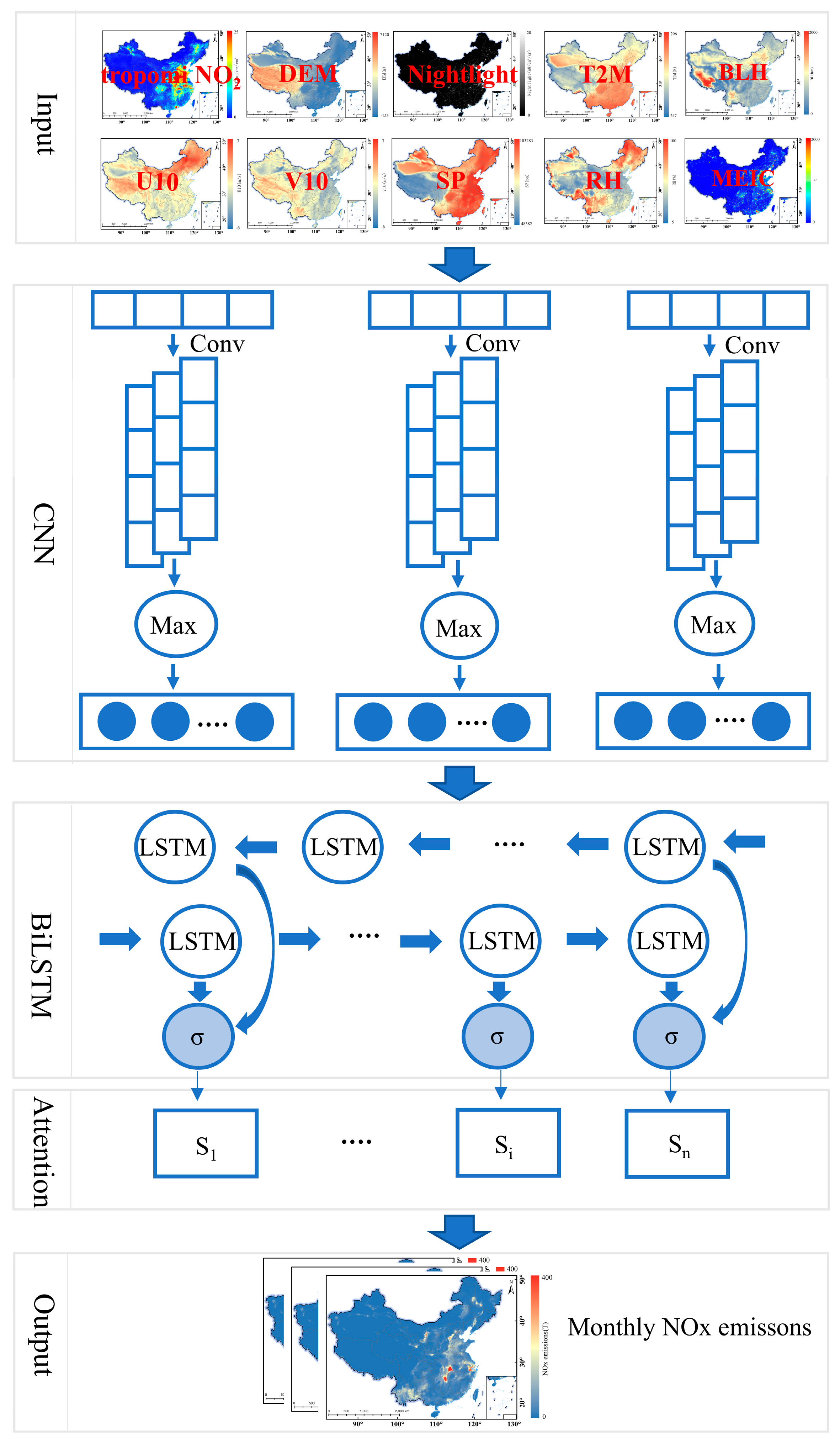
2.4.2. CNN-BiLSTM-ATT Model

The Convolutional Neural Network (CNN) model, first proposed by LeCun in 1998, is highly effective in feature extraction, addressing the limitations of other network models in this regard. The accuracy of feature extraction directly influences the prediction accuracy. The CNN model [43] consists of five primary modules: the input layer, which receives the original data; the convolutional layer, which extracts key features and serves as the core component of the model; the pooling layer, which reduces the data’s dimensionality; the fully connected layer, responsible for classifying the processed data; and the output layer, which generates the final results. The Long Short-Term Memory (LSTM) network [44], proposed by Hochreiter and Schmidhuber in 1997, is a variation of the Recurrent Neural Network (RNN) model. Experimental results demonstrate that the LSTM model excels in handling multivariate, multi-input, and large-scale data predictions, particularly in time series forecasting. The LSTM model consists of three gates and a memory cell: the input gate stores incoming data, the forget gate selectively discards irrelevant information, the memory cell retains important features, and the output gate produces the current state. A key advantage of the LSTM network is its ability to forget less relevant historical information, freeing up the network capacity and addressing the limitations of traditional RNN. The memory function within the LSTM model not only captures the temporal dynamics of NOx data but also accurately models the nonlinear relationships between emissions and input data, leading to superior prediction performance and higher accuracy.
To further enhance the model performance, a hybrid CNN-BiLSTM-ATT model is proposed, incorporating Bidirectional Long Short-Term Memory (BiLSTM) [45,46,47] and an attention mechanism on top of CNN and LSTM. BiLSTM enables the model to simultaneously learn temporal features from both forward and reverse time dimensions, while the attention mechanism improves the model’s ability to focus on key features by dynamically assigning weights. This hybrid approach excels in time series data analysis, enabling the more accurate capture of the patterns in NOx emissions. The CNN-BiLSTM-ATT model consists of an input layer, a CNN layer, a BiLSTM layer, an attention layer, and an output layer. First, the data are processed and resampled to a uniform resolution of 0.05° × 0.05°, followed by spatiotemporal matching to construct the dataset, which is then fed into the model through the input layer. The CNN layer is responsible for extracting spatial features from the input data. Upon entering the model, the data first pass through a convolutional layer, where key parameters—including the number of input and output channels, kernel size, and padding—are set to capture local spatial feature patterns effectively. Following this, a max-pooling layer is applied for downsampling, which not only reduces data dimensionality and computational complexity but also enhances the extraction of primary spatial features. However, the features extracted by the CNN cannot be directly used as input for the BiLSTM network due to differences in data format and dimensionality. To address this issue, the CNN output is transformed into a sequential format suitable for BiLSTM processing, enabling the seamless integration of spatial features into the subsequent temporal feature extraction. The attention mechanism further refines the output of the BiLSTM by performing a nonlinear transformation to compute attention scores for each time step. These scores reflect the relative importance of different time steps within the current task. A softmax function is then applied to normalize the scores into attention weights, ensuring that weight allocation is directly influenced by the intrinsic characteristics of the input data rather than being predetermined or arbitrary. This approach enhances the logical consistency of weight assignment and improves interpretability. When handling spatial features, the model dynamically assigns weights to different geographical regions based on data characteristics, allowing it to focus on spatial areas with a greater impact on the results. This adaptive weighting mechanism enables the model to better capture spatiotemporal variations and effectively process complex spatiotemporal patterns. Figure 1 illustrates the process. Before training the model, it is important to normalize the data to improve training stability and accelerate convergence. In this study, the Min–Max Scaling method was applied to scale both the input features and target variables to the range [0, 1], ensuring consistency in the numerical scales of different variables. During the model training process, the following steps were undertaken to optimize the model. First, the dataset was divided into a training set, a validation set, and a test set to ensure the model’s generalization ability and effectiveness. The training set was used to learn the model parameters, the validation set monitored the training process and hyperparameter tuning, and the test set evaluated the final performance. During training, the model weights were updated using the backpropagation algorithm and an optimizer to minimize the mean squared error (MSE) loss function. The Adam optimizer was employed, with the learning rate scheduled to improve the model’s stability and convergence speed. To further enhance the model’s performance, custom hyperparameter settings were used during training, including the configuration of the LSTM hidden layer size, number of layers, and fully connected layers. Additionally, to assess the model’s effectiveness, the validation and test sets were used for repeated evaluations. Various evaluation metrics, including MSE, root mean squared error (RMSE), MAE, and correlation coefficient R, were employed to comprehensively measure the model’s prediction accuracy and generalization ability.

3. Results

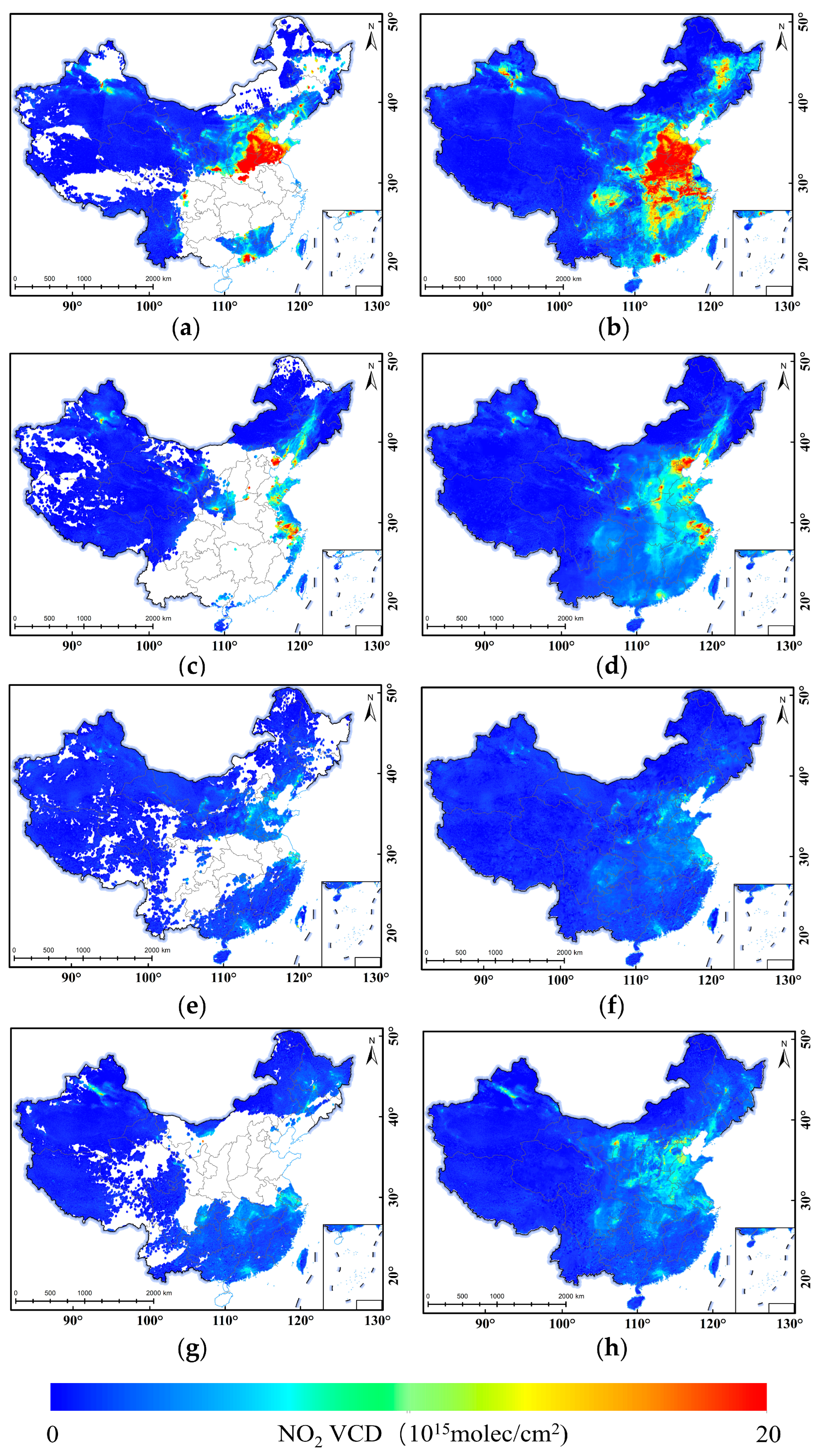
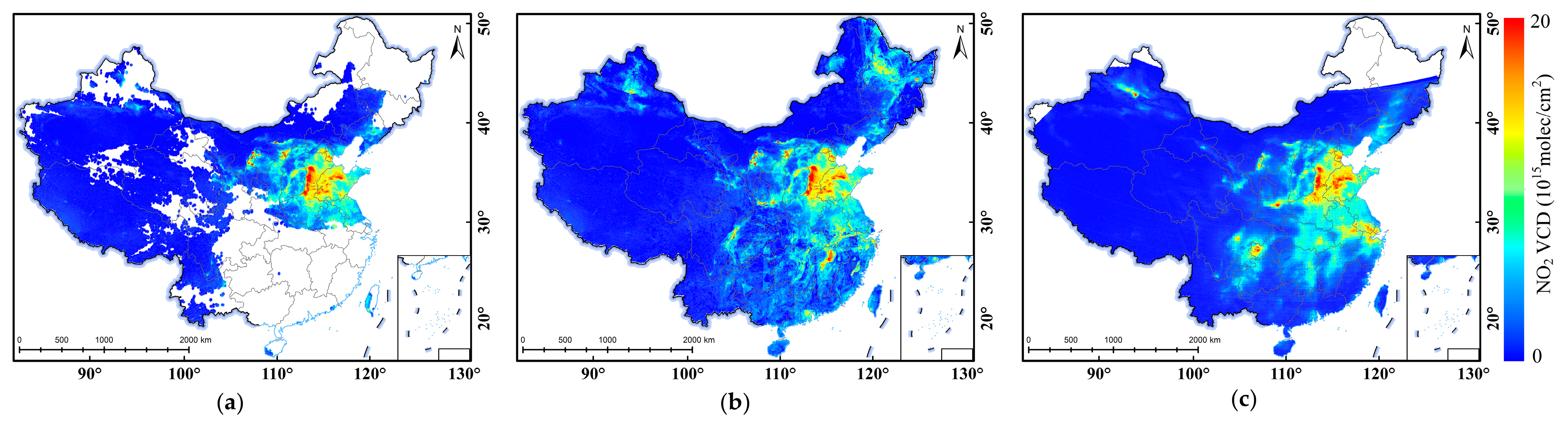
3.1. Gap Filling of Tropospheric NO2 VCD

3.1.1. Daily NO2 VCD and Verification

In this study, the tropospheric NO2 VCD data were spatially and temporally matched with meteorological and ground elevation data to create a comprehensive dataset. The LightGBM model was then employed to estimate the missing values, with a monthly model implemented due to the large amount of tropospheric NO2 data. To analyze the experimental results, the NO2 VCD values before and after gap filling were selected for 5 January, 5 April, 5 July, and 5 October 2021. As shown in Figure 2, the NO2 VCD is higher in the central and eastern regions, with the southwestern region exhibiting the lowest VCD. The spatial boundary between the filled values and the original data is smooth and consistent, and the spatial distribution aligns with prior knowledge of NO2 VCD in China, with higher levels observed in East China and the Beijing–Tianjin–Hebei region. Seasonal analysis revealed that NO2 VCD was higher in winter and lower in summer. This variation is influenced by multiple factors: the lower winter temperatures and unfavorable meteorological conditions hinder the dispersion of pollutants, leading to the accumulation of NO2 in the atmosphere. Additionally, increased heating and industrial emissions during winter further elevate NO2 density. In contrast, warmer temperatures and more sunlight in the summer promote photochemical reactions that convert NO2 into other substances such as ozone, while enhanced atmospheric convection facilitates the diffusion of pollutants, resulting in lower NO2 density during the summer months.
The performance of the tropospheric NO2 estimation model for January, April, July, and October 2021 was assessed using R2, MAE, and RMSE metrics to provide a clearer understanding of the model’s performance across different months and to evaluate its accuracy. Figure 3 shows the correlation between the predicted NO2 VCD and observations from TROPOMI for January, April, July, and October 2021. Specifically, the R2 value for January was 0.95, indicating a high degree of accuracy in the model’s estimates for that month. For April and July, the R2 values were 0.96, reflecting stable performance and a strong correlation between the predicted and actual values. In October, the R2 slightly decreased to 0.92, yet remained relatively high, suggesting that the model maintained strong performance across varying seasons and demonstrated both adaptability and accuracy. Further analysis of the MAE and RMSE metrics reveals that, for January, the MAE was approximately 0.17 × 10¹⁵ molec/cm2, while, in April and July, the MAE values were 0.18 × 10¹⁵ molec/cm2 and 0.17 × 10¹⁵ molec/cm2, respectively. However, in October, the MAE increased to 0.32 × 10¹⁵ molec/cm2, indicating a larger average absolute error during that month. This increase may be attributed to specific atmospheric conditions or variations in the data distribution. Regarding RMSE, it was 0.2 × 10¹⁵ molec/cm2 in January, approximately 0.3 × 10¹⁵ molec/cm2 in April and July, and increased to 0.5 × 10¹⁵ molec/cm2 in October. These values suggest that, particularly in October, the prediction error was more significant, likely due to local climatic variations or the complex distribution pattern of NO2. These metrics offer a clear visual representation of the model’s performance across different months. Overall, the model exhibited high accuracy in January, April, July, and October. Notably, for the NO2 VCD test set spanning 2019 to 2023, the model achieved an R2 value above 0.83 in all instances, highlighting the model’s stability and strong performance over time, with effective estimation and forecasting of NO2 VCD.
To further verify the accuracy of NO2 estimation in areas where TROPOMI NO2 data are missing, this study utilized NO2 VCD data from the GEMS sensor as an independent reference. Specifically, we evaluated the accuracy of the gap-filling method for missing NO2 VCD on 1 December 2022. As shown in Figure 4, the NO2 VCD distribution for that date is presented. Figure 4a illustrates the original TROPOMI data before gap filling, Figure 4b displays the full-coverage NO2 VCD obtained after LightGBM filling, and Figure 4c presents the NO2 VCD provided by GEMS. While some differences exist in specific values and distribution details, the overall trend in Figure 4b aligns well with Figure 4c, demonstrating a reasonable degree of consistency. This further supports the effectiveness of the LightGBM-based gap-filling method in restoring the NO2 VCD distribution. Furthermore, Figure 5 shows the relationship between the NO2 VCD filled in 2022 and the NO2 VCD observed by GEMS to further assess the reliability of the gap-filling approach. The results indicate a strong correlation between the two datasets, with an R2 of 0.72. This finding suggests that the filled NO2 data closely align with the GEMS observations, providing strong evidence for the validity and reliability of the gap-filling method.

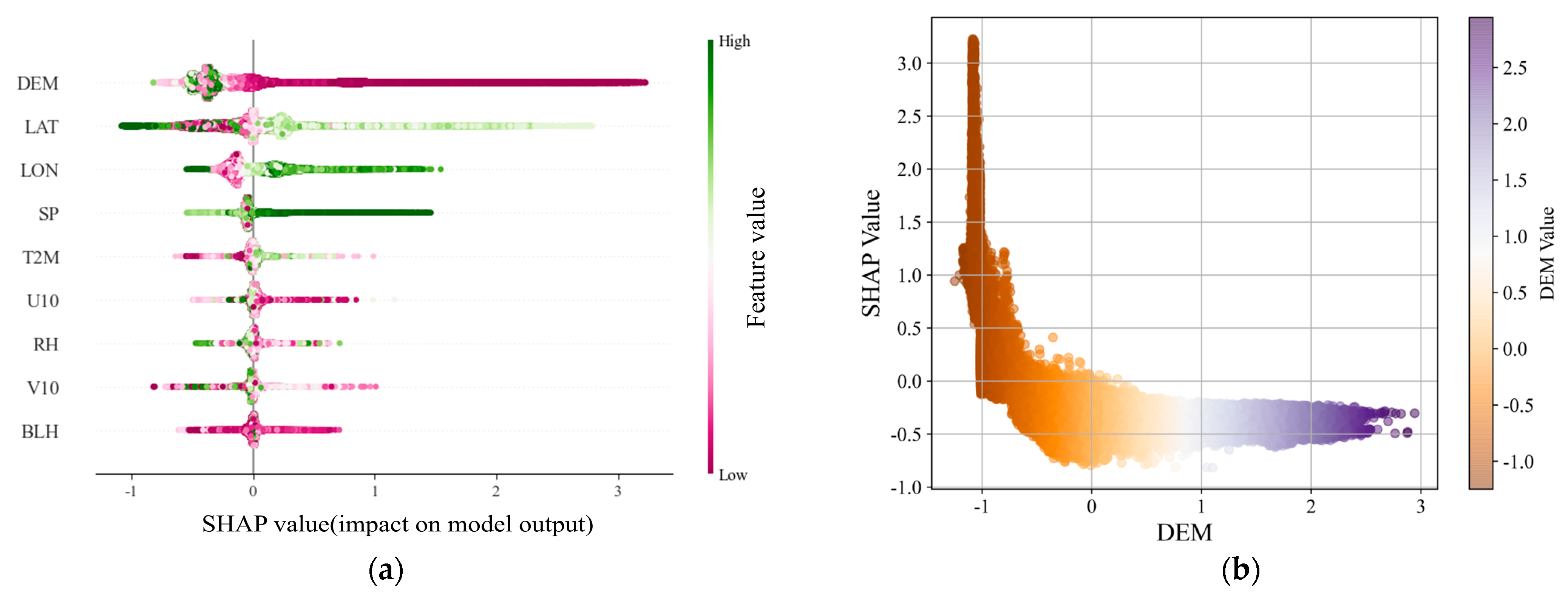
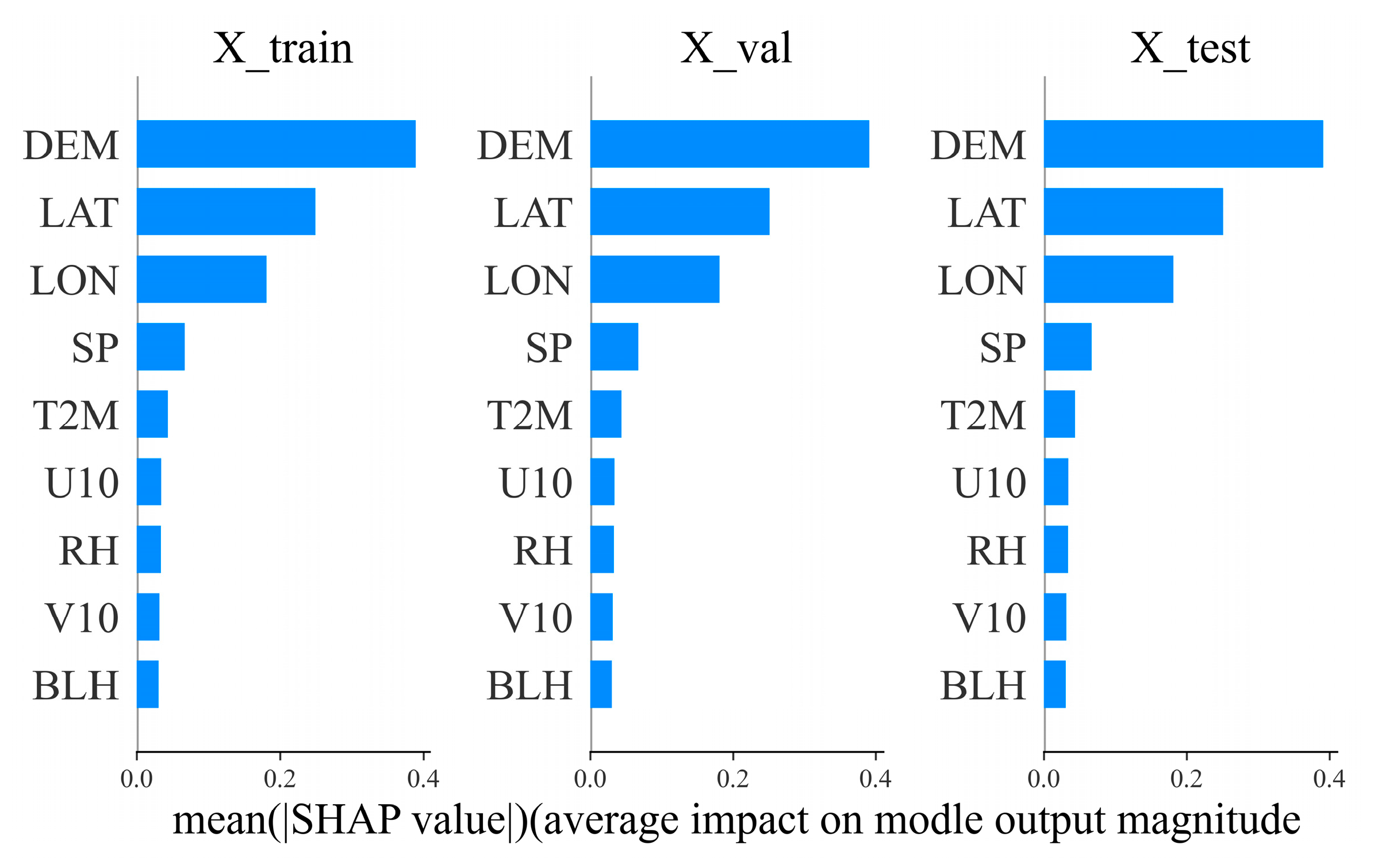
3.1.2. Analysis of Feature Contributions Using SHAP Values

SHAP (Shapley Additive Explanations) is a model interpretation method grounded in game theory, designed to explain machine learning models by quantifying the contribution of features to prediction outcomes. It calculates the marginal contribution of each feature across various feature combinations using Shapley values, ensuring consistent and fair interpretation.
The January model was selected to analyze the contribution and importance of each feature. The influence of each feature on the tropospheric NO2 VCD estimation model was quantified using SHAP values [48]. Figure 6a illustrates the contribution of different features to the model output and their directional influence. Points further to the right indicate a stronger positive impact of the feature on the model output, while points further to the left indicate a greater negative impact. Features ranked higher have a more substantial influence on the model. It can be observed that the SHAP value for DEM is notably large, highlighting its significant impact on NO2 VCD predictions. This suggests that terrain height plays a critical role in the model, potentially due to its effect on the diffusion and accumulation of NO2. The SHAP values for latitude (LAT) and longitude (LON) are secondary, emphasizing the importance of spatial location in estimating the NO2 concentration. This is likely due to the direct influence of geographical position on the sources and distribution of NO2. Meteorological conditions, including SP, T2M, U10, and RH, also have considerable impact on the model’s predictions. The SHAP values of these features reflect their varying effects on NO2 concentration estimations under different meteorological conditions, underscoring the key role of atmospheric conditions in the estimation process. Although the SHAP value for BLH is smaller, it remains important for understanding the vertical distribution of NO2 in the upper atmosphere. Figure 6b illustrates how DEM affects the model results, and when the DEM value is low, it has a strong positive effect on the model output (the SHAP value is significantly positive). When the DEM value is high, it has a negative effect on the model output. Figure 7 shows the mean absolute SHAP value of each feature on the training set, test set, and validation set. The higher the mean absolute value of the SHAP value, the more important the feature is to the model output. The consistency of the mean absolute SHAP values across the training, test, and validation sets suggests that the model’s feature importance evaluation remains stable across different datasets. This stability indicates that the model’s reliance on features is consistent and that the dataset distribution differences are minimal, which enhances the model’s generalization ability. Furthermore, this consistency implies appropriate feature selection and demonstrates the model’s robustness and stability across different environments.

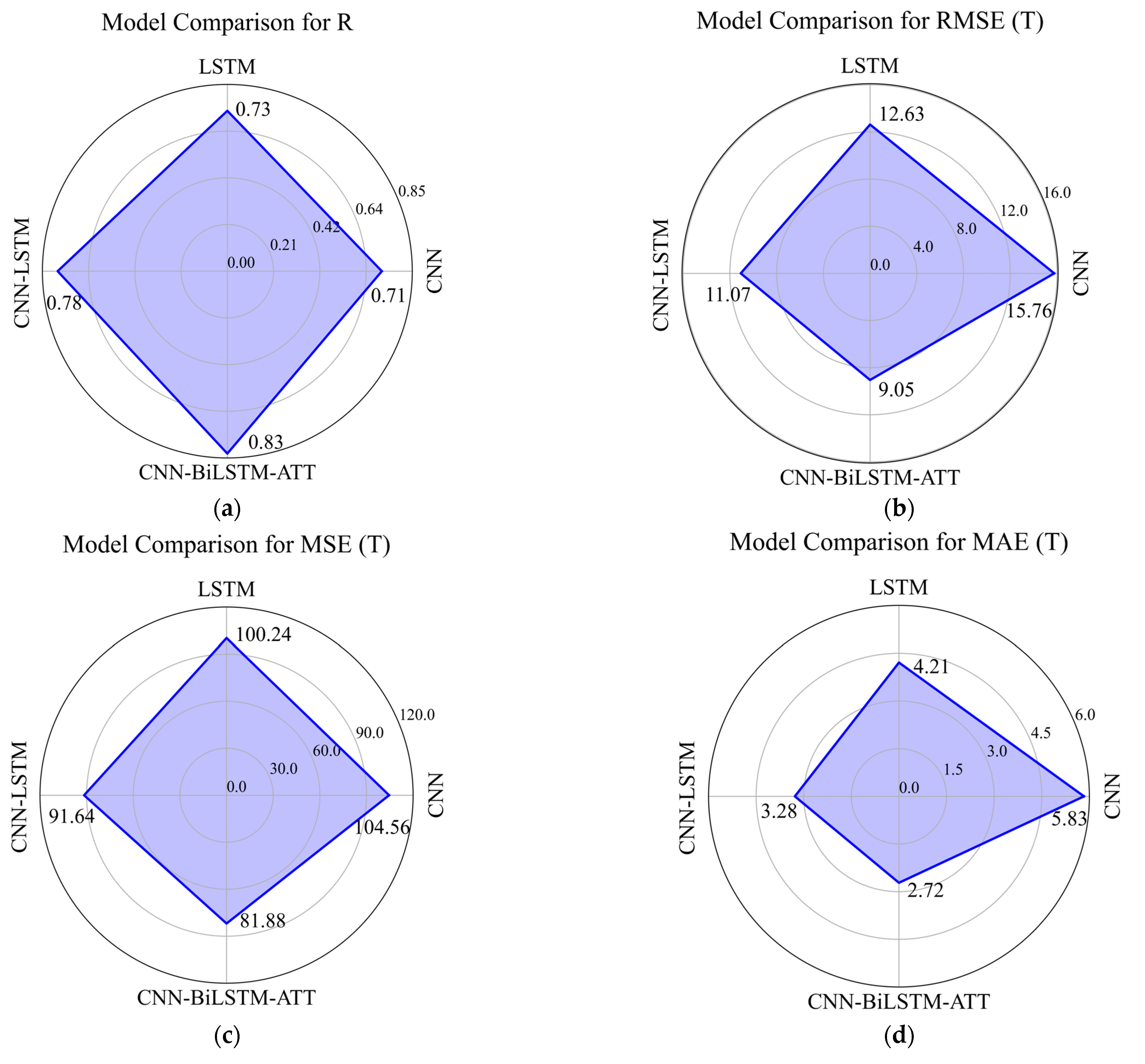
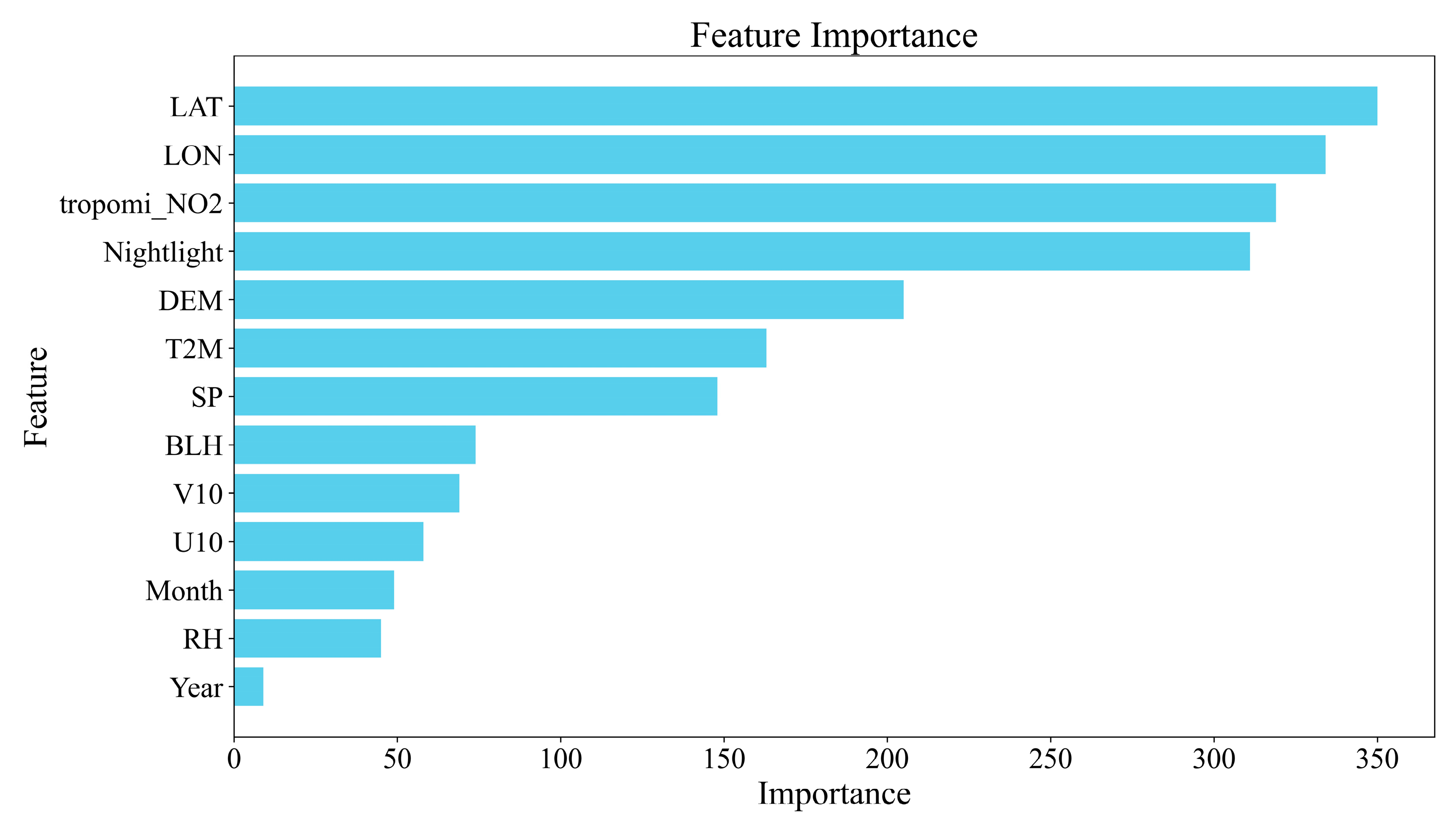
3.2. Model Comparison and Feature Importance

The complete tropospheric NO2 data were derived by filling in the daily NO2 VCD from 2019 to 2023. Subsequently, the meteorological data, DEM data, and nightlight data were temporally and spatially matched to construct a dataset. Using the 2019–2020 emission inventory, combined with influencing factors, NOx emissions for the years 2021 to 2023 were estimated, and the monthly NOx emission inventory for this period was constructed.
In the experiment, the CNN, LSTM, and CNN-LSTM models were compared with the CNN-BiLSTM-ATT model. These models were selected owing to their unique strengths in processing data. The CNN model was used primarily for its ability to capture spatial relationships and patterns in data, making it suitable for tasks where the spatial distribution of the data is crucial. The LSTM model, in contrast, was selected for its ability to handle sequential data and temporal dependencies. By combining these two models, the CNN-LSTM model uses the spatial feature extraction of CNN and the time series learning of LSTM to explore whether it will better analyze and process data and improve the estimation accuracy. The Bidirectional LSTM component enables the model to capture both past and future temporal dependencies by processing data in both forward and backward directions. The attention mechanism allows the model to focus on the most relevant parts of the input sequence, improving its ability to handle long sequences and better capture inter-feature relationships. The CNN-BiLSTM-ATT model combines Bidirectional LSTM and attention mechanism to explore whether the performance can be further improved.
Model performance was assessed using several indicators, including R, RMSE, MSE, and MAE. Figure 8 shows the radar plots that compare the performance of these models across these indicators. The R measures the strength and direction of the linear relationship between the true and estimated values. It is a key metric for evaluating the accuracy of model estimation, as it intuitively reflects the degree of linear correlation between the model’s estimates and the true values. A higher R value indicates a better fit between the model’s NOx emission estimates and the true values. The R value of the CNN-BiLSTM-ATT model reached 0.83, significantly higher than that of the CNN model (0.71), the LSTM model (0.73), and the CNN-LSTM model (0.78). This clearly demonstrates that the CNN-BiLSTM-ATT model is more effective at capturing the linear relationship between the true and estimated values and can generate estimates closer to the true values based on the input data. RMSE, MSE, and MAE are metrics used to measure the error between the model’s estimates and the true values. RMSE calculates the square root of the squared estimation errors, amplifying the influence of larger errors. MSE represents the average of the squared errors, again giving more weight to larger errors, while MAE is the average of the absolute errors, treating all errors equally. In these metrics, the CNN-BiLSTM-ATT model performed well. Its RMSE of 9.05 is lower than that of the CNN model (15.76), the LSTM model (12.63), and the CNN-LSTM model (11.07). The MSE of 81.88 is lower than that of the CNN model (104.56), the LSTM model (100.24), and the CNN-LSTM model (91.64), while the MAE of 2.72 outperforms the CNN model (5.83), the LSTM model (4.21), and the CNN-LSTM model (3.28). These results highlight that the CNN-BiLSTM-ATT model produces smaller errors and higher estimation accuracy in its predictions.
To investigate the enhancement effect of the attention mechanism on the model performance, we conducted ablation experiments by removing the attention mechanism from the CNN-BiLSTM-ATT model. The results are shown in Table 2. The R value of the CNN-BiLSTM-ATT model with the attention mechanism reached 0.83, while the R value of the CNN-BiLSTM model without the attention mechanism was 0.80. This difference indicates that the attention mechanism helps the model more effectively capture the linear relationships between variables, enabling it to more accurately reflect the correlation between input features and target variables, thereby improving the model’s estimation accuracy. The RMSE of the CNN-BiLSTM-ATT model was 9.05, with a MSE of 81.88, while the model without the attention mechanism had an RMSE of 10.71 and a MSE of 87.36. The lower RMSE and MSE values suggest that the model with the attention mechanism has a smaller deviation between the estimated and actual values, allowing it to more precisely approximate the true values when processing the data, thus highlighting the significant role of the attention mechanism in improving estimation accuracy. Furthermore, the MAE of the CNN-BiLSTM-ATT model was 2.72, lower than that of the CNN-BiLSTM model, which was 3.02. This suggests that the attention mechanism reduces the average error across samples, leading to a better overall model performance and greater adaptability to different data characteristics and changes.
The importance of each feature in the model was then analyzed, as shown in Figure 9, which ranks the features by their contribution to the estimation of NOx emissions. Latitude LAT and longitude LON were identified as the most important features, underscoring the decisive role of geographical location in the distribution of NOx emissions. Additionally, tropomi NO2 and Nightlight reflect satellite observations of atmospheric NO2 and the impact of human activities, respectively. These findings highlight a strong correlation between human activity intensity and NOx emissions. The importance of the DEM to NOx distribution may be attributed to the influence of terrain height on pollutant dispersion. Meteorological variables such as T2M, SP, BLH, V10, and U10 play a critical role in the diffusion, transformation, and accumulation of NOx. These factors capture the complex interactions between atmospheric conditions and pollutant concentrations. Together, these characteristics underscore the multifaceted roles of geographical location, meteorological conditions, human activities, and temporal factors in the distribution and variability of NOx, thereby providing a scientific foundation for modeling and analysis.

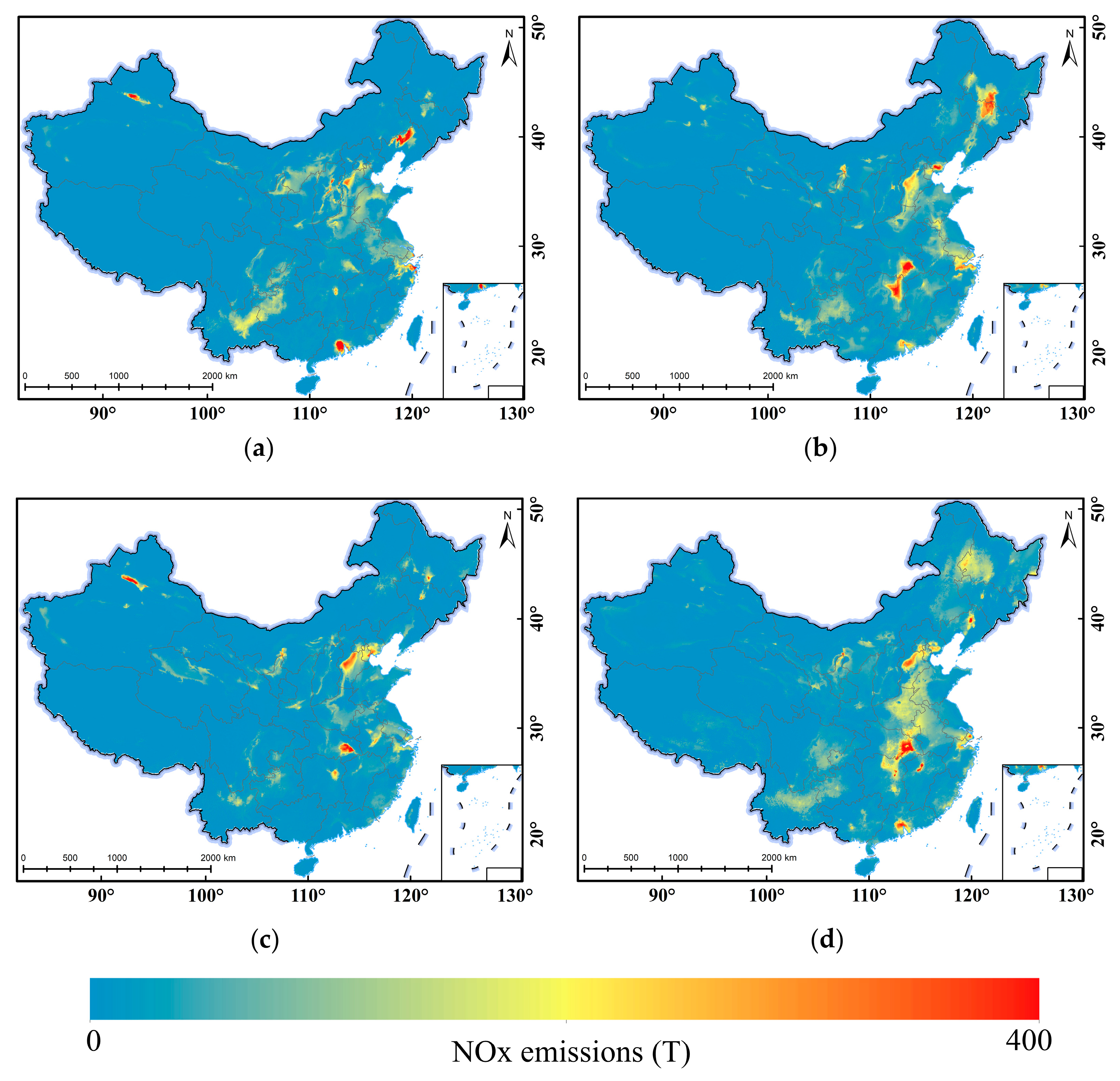
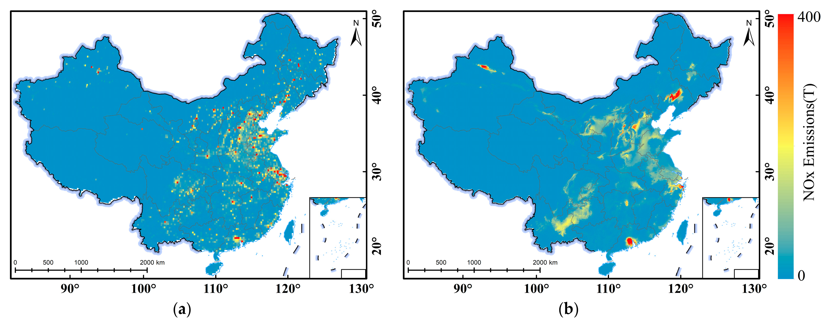
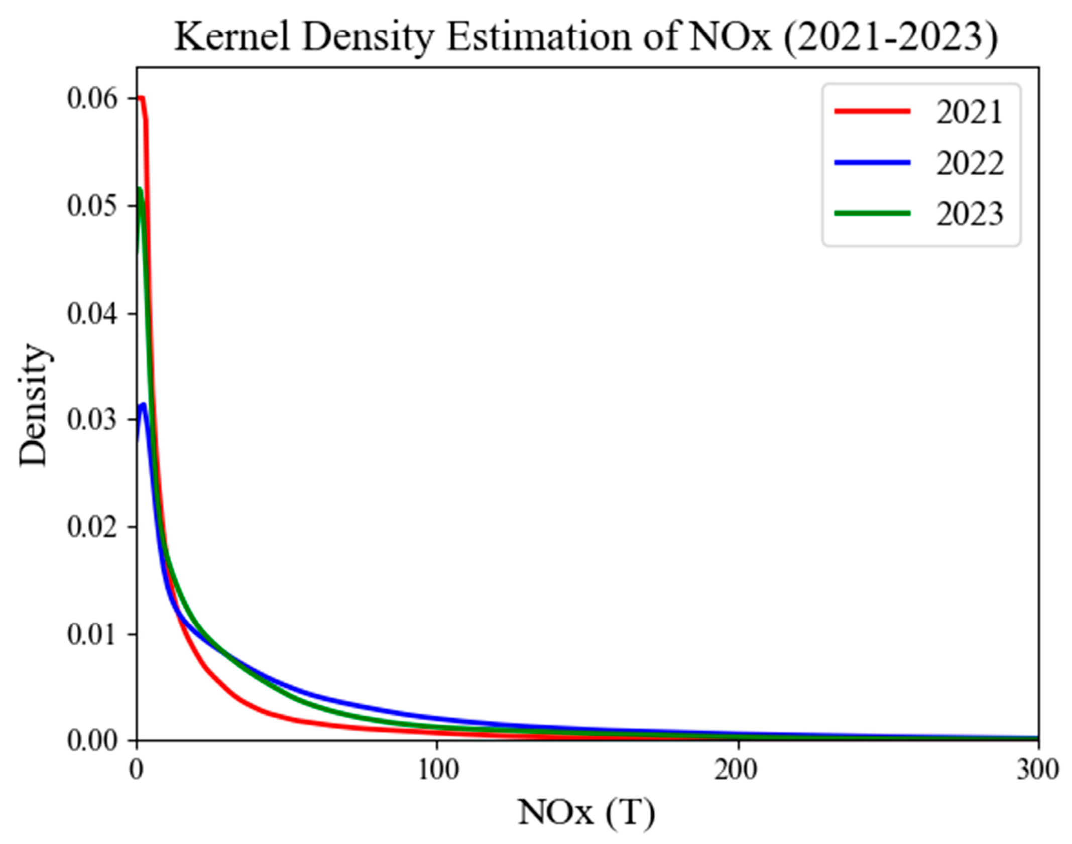
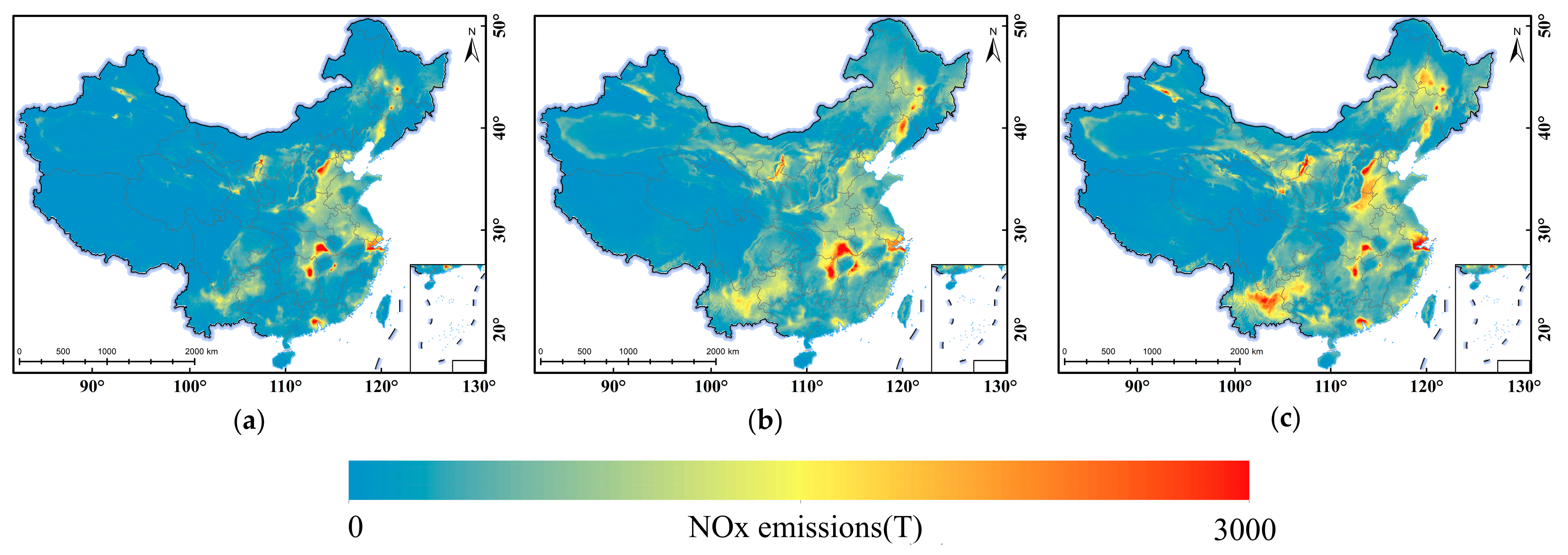
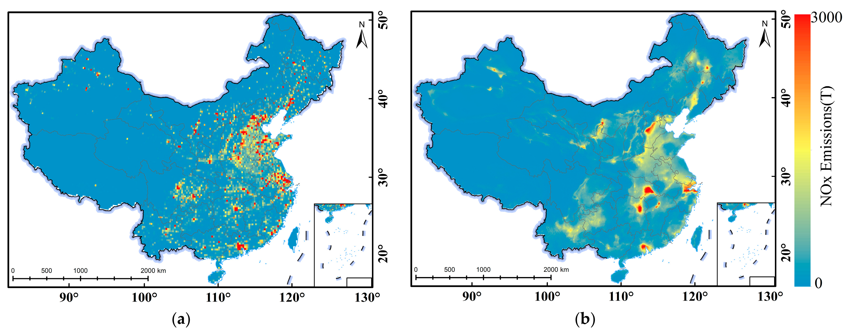
3.3. Monthly NOx Emissions Estimation

Figure 10 illustrates NOx emissions for January, April, July, and October 2021. It is evident that high emission values are less frequent in January and July, while they are more pronounced in April and October, reflecting the temporal variability and spatial distribution characteristics of NOx emissions. In January, NOx emissions are relatively low, primarily due to cold weather, which reduces industrial and transportation activities, leading to a slowdown in economic activities. Similarly, emissions in July remain low. Despite the high summer temperatures and increased demand for air conditioning, the overall NOx emissions in July are still lower than in winter due to reduced heating demands. Additionally, strong winds and favorable atmospheric dispersion conditions facilitate the diffusion of pollutants. In contrast, NOx emissions are higher in April and October. In April, rising spring temperatures stimulate industrial activities and transportation, while increased energy consumption leads to higher emissions. At the same time, the poor atmospheric stability during spring hinders the dispersion of pollutants. In October, as autumn begins, the use of heating devices in some regions increases the consumption of coal and other fuels. Moreover, heightened transportation and agricultural activities lead to elevated NOx emissions. The limited atmospheric stability in autumn further exacerbates pollutant accumulation, resulting in even higher emissions.
The Emission Database for Global Atmospheric Research (EDGAR) is a widely recognized global emissions inventory that provides data on greenhouse gases and air pollutants. In this study, the estimated monthly NOx emissions for 2021 were compared with those from EDGAR to assess emission trends. As shown in Figure 11, emissions fluctuate from month to month, with minimal differences between some months, such as June and July, and significant variations between others, such as November and December. The comparison reveals that, although the estimates are generally slightly higher than those from EDGAR, the overall trend—whether increasing or decreasing—remains consistent across the two datasets. Specifically, emissions were lower in June, July, and August, while higher levels were observed in October, November, and December. This pattern suggests seasonal variations in NOx emissions, with warmer months typically associated with lower emissions and colder months experiencing higher emissions, potentially due to factors such as energy consumption, transportation, and meteorological conditions.
Figure 12 illustrates the NOx emission distribution in January 2019 at a 0.25° × 0.25° resolution and the estimated NOx emission distribution in January 2021 at a 0.05° × 0.05° resolution. Despite differences in spatial resolution, the overall emission patterns in both maps exhibit a high degree of agreement, particularly in key emission hotspots such as major cities and industrial areas. This consistency suggests that the estimation model effectively captures the spatial distribution of NOx emissions. The finer resolution of the estimated NOx emissions for 2021 offers a more detailed representation of spatial variation. These higher-resolution estimates provide a smoother, more continuous emission gradient compared to the coarser 2019 distribution, minimizing the potential aggregation effect caused by coarse grid averaging. The estimated 2021 distribution also reveals improved spatial coherence and a more gradual transition of emission hotspots to the surrounding areas, demonstrating that the model reduces artificial noise and discontinuity, thereby enhancing the credibility of the estimation method.
This study investigates the monthly NOx emissions from Jiangxi, Hubei, Hebei, and Shandong Provinces in 2022, with the total monthly emissions for these regions calculated in Figure 13. Jiangxi, an inland province in Southern China, is primarily driven by agriculture, light industry, and tourism, with a relatively low proportion of heavy industry, resulting in comparatively low NOx emissions. Hubei, with its well-developed industrial base, particularly in steel, cement, and fertilizer production, experiences higher NOx emissions. Additionally, Hubei’s transportation system, being a key province in the middle reaches of the Yangtze River, contributes significantly to NOx emissions. Hebei, a major steel production hub, has heavy industrial activities, such as steel and cement production, which are significant sources of NOx emissions. Shandong, one of the most economically developed provinces in China, hosts a wide range of industries, including steel, fertilizer, and chemicals. The intensity of industrial activities in Shandong makes it a major contributor to NOx emissions.
In summary, the NOx emissions in these four provinces are influenced by factors such as industrialization, energy structure, and transportation. While each province exhibits distinct emission patterns, industrial activities and energy consumption remain the primary sources of pollution. To mitigate NOx emissions, promoting clean energy, improving transportation infrastructure, and enhancing pollution control measures are essential strategies in these regions.

4. Discussion

Kernel density estimation (KDE) curves for NOx emissions in the 0.05° × 0.05° regions from 2021 to 2023 were analyzed to represent the probability density distribution of NOx emissions over the years. As shown in Figure 14, the distribution of NOx emissions is highly skewed, with the majority of the data concentrated in the 0–100 T range. As emissions increase, the density decreases sharply, approaching zero in high-emission areas (above 100 T). The red, blue, and green colors in the figure represent the emissions distribution for 2021, 2022, and 2023, respectively. Notably, the curves for all three years exhibit similar shapes, indicating that the statistical profile of NOx emissions remained relatively stable throughout the three-year period. This distribution is likely attributable to the inherent characteristics of the emissions data, which are typically influenced by factors such as population density, industrial activities, and transportation emissions. Regions with low emission values often correspond to areas with limited industrial or rural activity, while high-emission zones are typically linked to densely industrialized or urbanized regions.
Additionally, we analyze the annual NOx emissions. Figure 15 illustrates that NOx emissions are consistently higher in the economically developed regions of Eastern and Central China, particularly in the Yangtze River Delta, Pearl River Delta, Beijing–Tianjin–Hebei region, and the industrially concentrated areas of Central China. Several factors contribute to the elevated NOx emissions in these regions. First, industrial activities play a critical role in driving high emissions. The Yangtze River Delta, Pearl River Delta, and Beijing–Tianjin–Hebei regions are home to numerous manufacturing, energy production, and heavy industries, such as steel, electricity, and chemicals, all of which emit substantial amounts of NOx during production processes. Second, transportation density is a significant contributor to high NOx emissions. The economically developed cities in these areas feature high volumes of motor vehicles, along with dense public transportation systems and logistics networks, making traffic emissions a major source of NOx. Additionally, the high population density in these regions exacerbates NOx emissions. As urbanization accelerates, energy consumption rises and traffic flows become more frequent, further amplifying NOx emissions. In contrast, the western regions of China exhibit relatively low NOx emissions, particularly in Tibet, Xinjiang, and other areas. This is mainly due to the low population densities and limited economic activities in these regions. Much of Western China is remote, with low levels of urbanization and minimal industrial and transportation activities, which results in lower NOx emissions. Additionally, the geographic characteristics of these regions also play a role in shaping NOx emissions. For example, Tibet and Xinjiang, characterized by high altitudes and vast deserts, have fewer human activities due to their harsh geographic conditions, leading to significantly lower NOx emissions compared to the more developed eastern and central regions. The analysis of annual NOx emissions reveals that higher emissions in the economically developed eastern and central regions are closely linked to industrialization, high transportation density, and population concentration. In contrast, the lower emissions in the western regions can be attributed to sparse populations, limited economic activities, and geographic conditions. These spatial disparities highlight the strong connection between regional economic development and environmental pollution, emphasizing the necessity for tailored pollution control measures that consider local conditions.
Figure 16 shows the NOx emissions distribution for 2020 (0.25° × 0.25° resolution) and the estimated NOx emissions distribution for 2021 (0.05° × 0.05° resolution). The spatial distribution of NOx emissions in 2021 remains consistent with that of 2020, with high-emission regions largely unchanged, indicating that the model effectively captures the major NOx emission sources and their spatial patterns. A notable improvement in 2021 is the enhanced spatial resolution, offering a more refined depiction of emission variations. Compared to the 2020 distribution, where emissions appear more aggregated due to the coarser grid, the 2021 results exhibit smoother transitions and more detailed local emission patterns. This higher resolution facilitates the better identification of spatial heterogeneity, particularly in regions with complex emission sources. The estimated NOx emissions in 2021 maintain the overall spatial characteristics of the 2020 distribution while benefiting from finer resolution, allowing for more precise and detailed emission assessments.
With the rapid development of China’s regional economy and infrastructure, the spatiotemporal characteristics of future NOx emissions are expected to undergo significant changes. Therefore, continuous emission monitoring and dynamic management will be essential for addressing future pollution challenges. As urbanization accelerates and industrial activities expand, the spatial distribution of emissions will likely shift, necessitating adaptive strategies for pollution control. Moreover, the R2 values of the monthly NO2 VCD model consistently exceeded 0.83, indicating strong model fitting performance. The CNN-BiLSTM-ATT model demonstrated superior performance in estimating NOx emissions, particularly when compared to other models, exhibiting higher estimation accuracy. This model effectively integrates spatiotemporal information from TROPOMI data and auxiliary variables such as meteorological data, enhancing both the accuracy and robustness of the estimations. Future research could focus on further optimizing the model by incorporating dynamic meteorological changes, diverse terrain types, and more refined spatiotemporal scales. Additionally, integrating more remote sensing data, such as PM2.5, CO, and other pollutants, alongside long-term emission monitoring datasets will improve the model’s generalization ability and further enhance its accuracy in forecasting future pollution trends. This study not only introduces a novel approach for air pollution monitoring and emission estimation but also provides valuable data support for future environmental management and policymaking.

5. Conclusions

In summary, the reconstruction of the full-coverage NO2 column through the fusion of TROPOMI, meteorological, and DEM data not only enhances the spatiotemporal resolution of the tropospheric atmosphere but also improves the accuracy of atmospheric pollution monitoring and emission estimation. The monthly model achieves an R2 value above 0.83, indicating strong fitting and predictive capabilities across different months. By combining the CNN-BiLSTM-ATT model, this approach effectively integrates NO2 column data with other auxiliary variables, yielding reliable estimates of NOx emissions from 2021 to 2023. Compared to traditional estimation models, this model demonstrates superior accuracy, with R = 0.83 and RMSE = 9.05 T, highlighting its advantages in large-scale emission estimation.
Furthermore, the reconstruction of NO2 VCD not only ensures the accuracy of spatiotemporal data but also includes a detailed analysis of the contribution and importance of each feature. Through SHAP value analysis, we identified key factors influencing NO2 VCD, providing deeper insights into the role of different variables in the model. A comparison of the estimated 2021 emission trends with EDGAR data showed high consistency in the overall trends, further validating the model’s accuracy and reliability. Finally, the spatiotemporal analysis conducted in this study revealed significant differences in NOx emissions across regions and seasons, highlighting the complex spatiotemporal characteristics and density distribution of NOx emissions.

Author Contributions

Conceptualization, K.C. and Y.S.; methodology, K.C. and Y.S.; software, Y.L.; validation, K.C., Y.S. and S.L.; formal analysis, M.F.; investigation, K.C.; resources, S.L.; data curation, M.F.; writing—original draft preparation, K.C. and Y.S.; writing—review and editing, S.L.; visualization, Y.L.; supervision, M.F.; project administration, S.L.; funding acquisition, K.C. and S.L. All authors have read and agreed to the published version of the manuscript.

Funding

This work was supported by the National Key R&D Program of China (2022YFF0606404), the National Natural Science Foundation of China (Grant No. U1804154), and the Natural Science Foundation of Henan Province, China (Grant No. 242300420215).

Data Availability Statement

Publicly available datasets were analyzed in this study. TROPOMI NO2 data can be found here: https://disc.gsfc.nasa.gov/ (accessed on 10 October 2024). MEIC data can be found here: http://meicmodel.org.cn (accessed on 2 October 2024). ERA5 data can be found here: https://cds.climate.copernicus.eu/#!/search?text=ERA5&type=dataset (accessed on 10 October 2024). DEM data can be found here: https://lpdaac.usgs.gov/products/astgtmv003/ (accessed on 14 October 2024). Nightlight data can be found here: https://eogdata.mines.edu/products/vnl/ (accessed on 12 October 2024).

Acknowledgments

The authors wish to acknowledge the National Aeronautics and Space Administration for supporting the present work.

Conflicts of Interest

The authors declare no conflicts of interest.

References

  1. Noone, K. Physics Today. In Atmospheric Chemistry and Physics: From Air Pollution to Climate Change, 3rd ed.; Seinfeld, J.H., Pandis, S.N., Eds.; Wiley: Hoboken, NJ, USA, 1998; Volume 51, pp. 88–90. [Google Scholar]
  2. Lelieveld, J.; Evans, J.S.; Fnais, M.; Giannadaki, D.; Pozzer, A. The contribution of outdoor air pollution sources to premature mortality on a global scale. Nature 2015, 525, 367–371. [Google Scholar] [CrossRef] [PubMed]
  3. Silver, B.; Conibear, L.; Reddington, C.L.; Knote, C.; Arnold, S.R.; Spracklen, D.V. Pollutant emission reductions deliver decreased PM2.5-caused mortality across China during 2015–2017. Atmos. Chem. Phys. 2020, 20, 11683–11695. [Google Scholar] [CrossRef]
  4. Seinfeld, J.H. Urban Air Pollution: State of the Science. Science 1989, 243, 745–752. [Google Scholar] [CrossRef] [PubMed]
  5. Logan, J.A. Nitrogen oxides in the troposphere: Global and regional budgets. J. Geophys. Res. Ocean. 1983, 88, 10785–10807. [Google Scholar] [CrossRef]
  6. Zhao, Y.; Qiu, L.P.; Xu, R.Y.; Xie, F.J.; Zhang, Q.; Yu, Y.Y.; Nielsen, C.P.; Qin, H.X.; Wang, H.K.; Wu, X.C.; et al. Advantages of a city-scale emission inventory for urban air quality research and policy: The case of Nanjing, a typical industrial city in the Yangtze River Delta, China. Atmos. Chem. Phys. 2015, 15, 12623–12644. [Google Scholar] [CrossRef]
  7. Zhao, Y.; Nielsen, C.P.; Lei, Y.; McElroy, M.B.; Hao, J. Quantifying the uncertainties of a bottom-up emission inventory of anthropogenic atmospheric pollutants in China. Atmos. Chem. Phys. 2011, 11, 2295–2308. [Google Scholar] [CrossRef]
  8. Chan, K.L.; Khorsandi, E.; Liu, S.; Baier, F.; Valks, P. Estimation of Surface NO2 Concentrations over Germany from TROPOMI Satellite Observations Using a Machine Learning Method. Remote Sens. 2021, 13, 969. [Google Scholar] [CrossRef]
  9. Geddes Jeffrey, A.; Martin Randall, V.; Boys Brian, L.; van Donkelaar, A. Long-Term Trends Worldwide in Ambient NO2 Concentrations Inferred from Satellite Observations. Environ. Health Perspect. 2016, 124, 281–289. [Google Scholar] [CrossRef]
  10. Zhan, Y.; Luo, Y.; Deng, X.; Zhang, K.; Zhang, M.; Grieneisen, M.L.; Di, B. Satellite-Based Estimates of Daily NO2 Exposure in China Using Hybrid Random Forest and Spatiotemporal Kriging Model. Environ. Sci. Technol. 2018, 52, 4180–4189. [Google Scholar] [CrossRef]
  11. Wang, W.; Liu, X.; Bi, J.; Liu, Y. A machine learning model to estimate ground-level ozone concentrations in California using TROPOMI data and high-resolution meteorology. Environ. Int. 2022, 158, 106917. [Google Scholar] [CrossRef]
  12. Qin, K.; Rao, L.; Xu, J.; Bai, Y.; Zou, J.; Hao, N.; Li, S.; Yu, C. Estimating Ground Level NO2 Concentrations over Central-Eastern China Using a Satellite-Based Geographically and Temporally Weighted Regression Model. Remote Sens. 2017, 9, 950. [Google Scholar] [CrossRef]
  13. Liu, R.; Ma, Z.; Liu, Y.; Shao, Y.; Zhao, W.; Bi, J. Spatiotemporal distributions of surface ozone levels in China from 2005 to 2017: A machine learning approach. Environ. Int. 2020, 142, 105823. [Google Scholar] [CrossRef] [PubMed]
  14. Huang, K.; Zhu, Q.; Lu, X.; Gu, D.; Liu, Y. Satellite-Based Long-Term Spatiotemporal Trends in Ambient NO(2) Concentrations and Attributable Health Burdens in China From 2005 to 2020. Geohealth 2023, 7, e2023GH000798. [Google Scholar] [CrossRef] [PubMed]
  15. Man, X.; Liu, R.; Zhang, Y.; Yu, W.; Kong, F.; Liu, L.; Luo, Y.; Feng, T. High-spatial resolution ground-level ozone in Yunnan, China: A spatiotemporal estimation based on comparative analyses of machine learning models. Environ. Res. 2024, 251, 118609. [Google Scholar] [CrossRef]
  16. Shao, Y.; Zhao, W.; Liu, R.; Yang, J.; Liu, M.; Fang, W.; Hu, L.; Adams, M.; Bi, J.; Ma, Z. Estimation of daily NO2 with explainable machine learning model in China, 2007–2020. Atmos. Environ. 2023, 314, 120111. [Google Scholar] [CrossRef]
  17. van der, A.R.J.; Mijling, B.; Ding, J.; Koukouli, M.E.; Liu, F.; Li, Q.; Mao, H.; Theys, N. Cleaning up the air: Effectiveness of air quality policy for SO2 and NOx emissions in China. Atmos. Chem. Phys. 2017, 17, 1775–1789. [Google Scholar] [CrossRef]
  18. Beirle, S.; Boersma, K.F.; Platt, U.; Lawrence, M.G.; Wagner, T. Megacity Emissions and Lifetimes of Nitrogen Oxides Probed from Space. Science 2011, 333, 1737–1739. [Google Scholar] [CrossRef]
  19. Liu, F.; Beirle, S.; Zhang, Q.; Dörner, S.; He, K.; Wagner, T. NOx lifetimes and emissions of cities and power plants in polluted background estimated by satellite observations. Atmos. Chem. Phys. 2016, 16, 5283–5298. [Google Scholar] [CrossRef]
  20. Zhang, J.; Van Der, A.R.J.; Ding, J. Detection and emission estimates of NOx sources over China North Plain using OMI observations. Int. J. Remote Sens. 2018, 39, 2847–2859. [Google Scholar] [CrossRef]
  21. Wang, Y.; Yuan, Q.; Li, T.; Zhu, L.; Zhang, L. Estimating daily full-coverage near surface O3, CO, and NO2 concentrations at a high spatial resolution over China based on S5P-TROPOMI and GEOS-FP. ISPRS J. Photogramm. Remote Sens. 2021, 175, 311–325. [Google Scholar] [CrossRef]
  22. Wu, Y.; Di, B.; Luo, Y.; Grieneisen, M.L.; Zeng, W.; Zhang, S.; Deng, X.; Tang, Y.; Shi, G.; Yang, F.; et al. A robust approach to deriving long-term daily surface NO2 levels across China: Correction to substantial estimation bias in back-extrapolation. Environ. Int. 2021, 154, 106576. [Google Scholar] [CrossRef] [PubMed]
  23. Wei, J.; Liu, S.; Li, Z.; Liu, C.; Qin, K.; Liu, X.; Pinker, R.T.; Dickerson, R.R.; Lin, J.; Boersma, K.F.; et al. Ground-Level NO2 Surveillance from Space Across China for High Resolution Using Interpretable Spatiotemporally Weighted Artificial Intelligence. Environ. Sci. Technol. 2022, 56, 9988–9998. [Google Scholar] [CrossRef] [PubMed]
  24. Grzybowski, P.T.; Markowicz, K.M.; Musiał, J.P. Estimations of the Ground-Level NO2 Concentrations Based on the Sentinel-5P NO2 Tropospheric Column Number Density Product. Remote Sens. 2023, 15, 378. [Google Scholar] [CrossRef]
  25. Cedeno Jimenez, J.R.; Pugliese Viloria, A.d.J.; Brovelli, M.A. Estimating Daily NO2 Ground Level Concentrations Using Sentinel-5P and Ground Sensor Meteorological Measurements. ISPRS Int. J. Geo-Inf. 2023, 12, 107. [Google Scholar] [CrossRef]
  26. Veefkind, J.P.; Aben, I.; McMullan, K.; Förster, H.; de Vries, J.; Otter, G.; Claas, J.; Eskes, H.J.; de Haan, J.F.; Kleipool, Q.; et al. TROPOMI on the ESA Sentinel-5 Precursor: A GMES mission for global observations of the atmospheric composition for climate, air quality and ozone layer applications. Remote Sens. Environ. 2012, 120, 70–83. [Google Scholar] [CrossRef]
  27. Wang, C.; Wang, T.; Wang, P.; Rakitin, V. Comparison and Validation of TROPOMI and OMI NO2 Observations over China. Atmosphere 2020, 11, 636. [Google Scholar] [CrossRef]
  28. Wang, Y.; Wang, J.; Zhou, M.; Henze, D.K.; Ge, C.; Wang, W. Inverse modeling of SO2 and NOx emissions over China using multisensor satellite data—Part 2: Downscaling techniques for air quality analysis and forecasts. Atmos. Chem. Phys. 2020, 20, 6651–6670. [Google Scholar] [CrossRef]
  29. Fioletov, V.; McLinden, C.A.; Griffin, D.; Theys, N.; Loyola, D.G.; Hedelt, P.; Krotkov, N.A.; Li, C. Anthropogenic and volcanic point source SO2 emissions derived from TROPOMI on board Sentinel-5 Precursor: First results. Atmos. Chem. Phys. 2020, 20, 5591–5607. [Google Scholar] [CrossRef]
  30. Bo, Z.; Dan, T.; Meng, L.; Fei, L.; Chaopeng, H.; Guannan, G.; Haiyan, L.; Xin, L.; Liqun, P.; Ji, Q. Trends in China’s anthropogenic emissions since 2010 as the consequence of clean air actions. Atmos. Chem. Phys. Discuss. 2018, 18, 14095–14111. [Google Scholar]
  31. Geng, G.; Liu, Y.; Liu, Y.; Liu, S.; Cheng, J.; Yan, L.; Wu, N.; Hu, H.; Tong, D.; Zheng, B.; et al. Efficacy of China’s clean air actions to tackle PM2.5 pollution between 2013 and 2020. Nat. Geosci. 2024, 17, 987–994. [Google Scholar] [CrossRef]
  32. Li, M.; Liu, H.; Geng, G.; Hong, C.; Fei, S. Anthropogenic emission inventories in China: A review. Natl. Sci. Rev. 2017, 4, 834–866. [Google Scholar]
  33. Bolan, S.; Padhye, L.P.; Jasemizad, T.; Govarthanan, M.; Karmegam, N.; Wijesekara, H.; Amarasiri, D.; Hou, D.; Zhou, P.; Biswal, B.K. Impacts of climate change on the fate of contaminants through extreme weather events. Sci. Total Environ. 2023, 909, 168388. [Google Scholar] [PubMed]
  34. Hersbach, H.; Bell, B.; Berrisford, P.; Hirahara, S.; Horányi, A.; Muñoz-Sabater, J.; Nicolas, J.; Peubey, C.; Radu, R.; Schepers, D.; et al. The ERA5 global reanalysis. Q. J. R. Meteorol. Soc. 2020, 146, 1999–2049. [Google Scholar] [CrossRef]
  35. Abrams, M.; Crippen, R.; Fujisada, H. ASTER global digital elevation model (GDEM) and ASTER global water body dataset (ASTWBD). Remote Sens. 2020, 12, 1156. [Google Scholar] [CrossRef]
  36. Fujisada, H.; Urai, M.; Iwasaki, A. Technical methodology for ASTER global DEM. IEEE Trans. Geosci. Remote Sens. 2012, 50, 3725–3736. [Google Scholar]
  37. Jiang, J.; Zhang, J.; Zhang, Y.; Zhang, C.; Tian, G. Estimating nitrogen oxides emissions at city scale in China with a nightlight remote sensing model. Sci. Total Environ. 2016, 544, 1119–1127. [Google Scholar]
  38. Xu, Y.; Zhang, W.; Huo, T.; Streets, D.G.; Wang, C. Investigating the spatio-temporal influences of urbanization and other socioeconomic factors on city-level industrial NOx emissions: A case study in China. Environ. Impact Assess. Rev. 2023, 99, 106998. [Google Scholar]
  39. Wei, J.; Li, Z.; Pinker, R.T.; Wang, J.; Sun, L.; Xue, W.; Li, R.; Cribb, M. Himawari-8-derived diurnal variations in ground-level PM2.5 pollution across China using the fast space-time Light Gradient Boosting Machine (LightGBM). Atmos. Chem. Phys. 2021, 21, 7863–7880. [Google Scholar] [CrossRef]
  40. Meng, Q. LightGBM: A Highly Efficient Gradient Boosting Decision Tree. In Proceedings of the Neural Information Processing Systems, Long Beach, CA, USA, 4–9 December 2017. [Google Scholar]
  41. Yao, T.E.; Lu, S.H.; Wang, Y.Q.; Li, X.H.; Ye, H.X.; Duan, Y.S.; Fu, Q.Y.; Li, J. Revealing the drivers of surface ozone pollution by explainable machine learning and satellite observations in Hangzhou Bay, China. J. Clean Prod. 2024, 440, 7. [Google Scholar] [CrossRef]
  42. Zhong, J.; Zhang, X.; Gui, K.; Wang, Y.; Che, H.; Shen, X.; Zhang, L.; Zhang, Y.; Sun, J.; Zhang, W. Robust prediction of hourly PM2.5 from meteorological data using LightGBM. Natl. Sci. Rev. 2021, 8, nwaa307. [Google Scholar] [CrossRef]
  43. Raccagni, S.; Sangiorgi, L.; Carnevale, C.; Nardi, S.D. Convolutional Neural Network to forecast complex systems: The nitrogen oxides concentration case. In Proceedings of the 2024 10th International Conference on Control, Decision and Information Technologies (CoDIT), Valletta, Malta, 1–4 July 2024; pp. 860–865. [Google Scholar]
  44. Yadav, H.; Thakkar, A. NOA-LSTM: An efficient LSTM cell architecture for time series forecasting. Expert Syst. Appl. 2024, 238, 122333. [Google Scholar] [CrossRef]
  45. Geng, D.; Wang, B.; Gao, Q. A hybrid photovoltaic/wind power prediction model based on Time2Vec, WDCNN and BiLSTM. Energy Convers. Manag. 2023, 291, 117342. [Google Scholar] [CrossRef]
  46. Kim, J.; Oh, S.; Kim, H.; Choi, W. Tutorial on time series prediction using 1D-CNN and BiLSTM: A case example of peak electricity demand and system marginal price prediction. Eng. Appl. Artif. Intell. 2023, 126, 106817. [Google Scholar] [CrossRef]
  47. Lei, L.; Shao, S.; Liang, L. An evolutionary deep learning model based on EWKM, random forest algorithm, SSA and BiLSTM for building energy consumption prediction. Energy 2024, 288, 129795. [Google Scholar] [CrossRef]
  48. Junaid, M.; Ali, S.; Eid, F.; El-Sappagh, S.; Abuhmed, T. Explainable machine learning models based on multimodal time-series data for the early detection of Parkinson’s disease. Comput. Methods Programs Biomed. 2023, 234, 107495. [Google Scholar] [CrossRef]
Figure 1. Schematic diagram of the CNN-BiLSTM-ATT model.
Remotesensing 17 01231 g001
Figure 2. NO2 VCD before and after gap filling on 5 January, 5 April, 5 July, and 5 October 2021: (a) before gap filling on 5 January 2021; (b) after gap filling on 5 January 2021; (c) before gap filling on 5 April 2021; (d) after gap filling on 5 April 2021; (e) before gap filling on 5 July 2021; (f) after gap filling on 5 July 2021; (g) before gap filling on 5 October 2021; (h) after gap filling on 5 October 2021.
Remotesensing 17 01231 g002
Figure 3. The correlation between predicted NO2 VCD and observations from TROPOMI for January, April, July, and October 2021: (a) January 2021; (b) April 2021; (c) July 2021; (d) October 2021.
Remotesensing 17 01231 g003
Figure 4. NO2 VCD on 1 December 2022: (a) TROPOMI NO2 VCD before gap filling; (b) TROPOMI NO2 VCD after gap filling; (c) GEMS NO2 VCD.
Remotesensing 17 01231 g004
Figure 5. Scatter plot of NO2 VCD with missing areas filled and GEMS NO2 VCD on 1 December 2022.
Remotesensing 17 01231 g005
Figure 6. SHAP values calculated based on the LightGBM-SHAP model: (a) SHAP value and feature influence direction; (b) the influence of DEM on the model.
Remotesensing 17 01231 g006
Figure 7. Mean absolute SHAP value on the training set, test set, and validation set.
Remotesensing 17 01231 g007
Figure 8. Comparison of the performance of CNN, LSTM, CNN-LSTM, and CNN-BiLSTM-ATT on R, RMSE, MSE, and MAE: (a) the performance of each model on the R; (b) the performance of each model on the RMSE; (c) the performance of each model on the MSE; (d) the performance of each model on the MAE.
Remotesensing 17 01231 g008
Figure 9. Ranking diagram of the importance of features to the model.
Remotesensing 17 01231 g009
Figure 10. Estimated NOx emissions in China for January, April, July, and October 2021: (a) January 2021; (b) April 2021; (c) July 2021; (d) October 2021.
Remotesensing 17 01231 g010
Figure 11. Comparison of monthly estimated and EDGAR NOx for 2021.
Remotesensing 17 01231 g011
Figure 12. NOx emission distribution for January 2019 and the estimated distribution for January 2021: (a) January 2019; (b) January 2021.
Remotesensing 17 01231 g012
Figure 13. Monthly emissions in four provinces: (a) Jiangxi; (b) Hubei; (c) Hebei; (d) Shandong.
Remotesensing 17 01231 g013
Figure 14. Kernel density estimation curves for NOx emissions from 2021 to 2023.
Remotesensing 17 01231 g014
Figure 15. Annual NOx emissions from 2021 to 2023: (a) 2021; (b) 2022; (c) 2023.
Remotesensing 17 01231 g015
Figure 16. NOx emission distribution for 2020 and the estimated distribution for 2021: (a) 2020; (b) 2021.
Remotesensing 17 01231 g016
Table 1. Source and information of the data used in this study.
DatasetVariableSpatial ResolutionTemporal ResolutionData Source
TROPOMITropospheric NO2 column5.5 km × 3.5 kmDailySentinel-5P
MeteorologyU10, V10, T2M RH, SP, BLH0.25° × 0.25°HourlyERA5
EmissionNOx0.25° × 0.25°MonthlyMEIC
TopographyDEM30 m × 30 m-ASTER GDEM
VIIRS DNBNightlight500 m × 500 mMonthlySNPP
Table 2. Comparison between the CNN-BiLSTM and CNN-BiLSTM-ATT models.
ModelRRMSEMSEMAE
CNN-BiLSTM0.8010.7187.363.02
CNN-BiLSTM-ATT0.839.0581.882.72
Disclaimer/Publisher’s Note: The statements, opinions and data contained in all publications are solely those of the individual author(s) and contributor(s) and not of MDPI and/or the editor(s). MDPI and/or the editor(s) disclaim responsibility for any injury to people or property resulting from any ideas, methods, instructions or products referred to in the content.

