Abstract
Satellite-derived aerosol optical depth (AOD) products from MODIS and VIIRS sensors are vital for monitoring global aerosol distributions. However, inconsistencies in quality control algorithms and spatial resolution introduce errors that complicate validation processes and reduce the accuracy of satellite-to-ground comparisons. This study proposes the “optimal” spatial matching method to minimize these errors and enable a more accurate evaluation of retrieval algorithm performance. Using AERONET ground observations from 2012 to 2021, MODIS and VIIRS AOD products were systematically validated with three spatial matching methods—“direct”, “average”, and “optimal”. Results demonstrate that the “optimal” method consistently outperformed the other methods by selecting pixel values. The study highlights significant quality control disparities across AOD products and demonstrates that high-resolution products, with purer pixels, achieve superior accuracy under the “optimal” method. These insights provide valuable guidance for optimizing dataset applications and refining aerosol retrieval algorithms.
1. Introduction
Atmospheric aerosols, composed of a mixture of solid or liquid particles suspended in the atmosphere, have both direct and indirect effects on climate [1]. These aerosols significantly influence the Earth’s energy balance [2], contribute to climate change [3,4], and impact human health [5,6]. Aerosols are widely distributed, exhibiting notable spatial and temporal variability [7], which requires quantitative measurements to thoroughly understand their effects on climate and related fields. Aerosol optical depth (AOD) quantifies the extent of solar radiation attenuation as it passes through an aerosol-containing atmospheric column and serves as a critical parameter in the radiative transfer equation, essential for simulating aerosol impacts on atmospheric radiation [8,9]. Ground-based AOD measurements provide accurate point observations but suffer from limited spatial coverage. To overcome this limitation, satellite retrievals have become the primary method for obtaining AOD data, offering much broader spatial coverage than ground-based stations [10].
The MODerate Resolution Imaging Spectroradiometer (MODIS) sensors, aboard Terra (2000) and Aqua (2002), are widely recognized and extensively used in numerous applications due to their long-term, globally comprehensive data record [11]. They have exceeded their initial five-year design life, recording data for over two decades and now exhibiting signs of aging. To ensure the continuity of long-term observational data, Visible Infrared Imaging Radiometer Suite (VIIRS) sensors, which are similar to MODIS, were deployed. One VIIRS sensor has been operational on the Suomi National Polar-Orbiting Partnership (SNPP) spacecraft since 2011, with another operational on NOAA-20 since 2017. These sensors not only extend the MODIS observational record but also improve its quality and coverage [12,13,14].
To retrieve AOD, three primary algorithms have been developed over land for the MODIS and VIIRS sensors. The Dark Target (DT) algorithm, referring exclusively to the land algorithm in this paper, is the earliest developed approach. It relies on fixed statistical relationships of surface reflectance between visible and shortwave infrared channels over vegetated or dark-soiled land (dark in the visible spectrum) [15]. Identifying dark target pixels within designated “retrieval boxes” is essential for the DT algorithm. In contrast, the Deep Blue (DB) algorithm relies more heavily on historical data. On bright surfaces, the blue spectral region is sufficiently darker than the long-wavelength region, enabling differentiation between the surface and dust plumes. The DB algorithm uses this characteristic by applying the minimum reflectance method to establish a static, pre-calculated surface reflectance database [16]. Both the DT and DB algorithms retrieve AOD based on the Lambertian surface assumption, utilizing single-orbit data. In contrast, the Multi-Angle Implementation of Atmospheric Correction (MAIAC) algorithm retrieves AOD based on a non-Lambertian surface assumption, incorporating multi-orbit data over a span of 3 to 16 days [17]. Each algorithm generates one or more associated scientific datasets. To expand coverage for climate research, the MODIS aerosol product includes a merged 10 km dataset (DTB), which combines DT and DB retrievals [18].
Ensuring dataset accuracy is critical during algorithm updates and applications in research. Therefore, appropriate methods must be employed to compare site measurements with satellite products to verify data reliability. Due to differences in measurement methods between satellite and ground-based instruments, their products vary in wavelength, time, and spatial coverage. In the early stages of MODIS product development, a method based on temporal and spatial window averaging was proposed to compare satellite datasets with ground-based observations, and the findings indicated that spatial window selection had a relatively minor effect on validation outcomes [19]. This method has since been widely applied in the validation of AOD products retrieved using the DT and DB algorithms in MODIS and VIIRS. Some studies have refined the temporal and spatial window sizes, employing approaches such as computing the average AOD value within a specified spatial window (weighted by distance or pixel count) for comparison with ground-based measurements [17,20,21,22,23,24,25,26]. Additionally, to mitigate the potential influence of residual clouds on validation results, further data filtering has been performed within spatial windows. For instance, during the validation of the MAIAC algorithm, a 20 × 20 km2 window was used to filter 1 km resolution AOD retrievals, and the highest 50% of AOD values were removed before averaging [17].
However, averaging methods can inherently introduce biases, particularly when extreme values arise due to undetected clouds [27,28]. While quality control measures in DT and DB products flag high-quality retrievals [29], the detection and removal of subpixel clouds remain particularly challenging [30,31]. Ideally, AOD algorithm validation should be conducted under cloud-free conditions. However, due to the contamination of subpixel clouds, validation based on averaging methods primarily reflects the accuracy of the product rather than the accuracy of the retrieval algorithm. A more robust validation approach is needed to better isolate algorithmic performance from quality control effects.
To ensure that validation results reflect the maximum achievable accuracy of these algorithms, we applied a new processing method to address this issue, aiming to minimize the influence of quality control procedures by selecting optimal values within a specified window. This study evaluates the accuracy of MODIS and VIIRS AOD products using ground-based observations from the global Aerosol Robotic Network (AERONET) from 2012 to 2021, presenting validation results based on various matching methods. Since most AERONET sites are situated on land, the comparison focuses exclusively on AOD products over land. In this paper, Section 2 introduces the datasets, Section 3 outlines the matching method and verification indicators, Section 4 discusses and analyses the results, and Section 5 provides a summary of the conclusions.
2. Data Description
2.1. Satellite AOD Datasets
The datasets used in this study are listed in Table 1, comprising a total of 13 datasets. MODIS Collection 6, released in 2016 for all atmospheric products, was followed by a minor update to Collection 6.1 in 2017. VIIRS DB Version 1 and DT Version 1 were released in 2018 and 2020, respectively, with updates to Version 1.1 in 2021 and Version 2.0 in 2023. The “Alias” column provides convenient references for these datasets throughout the study. For the MAIAC, retrievals from the Terra and Aqua satellites are separated and labeled as MOD(MAIAC) and MYD(MAIAC), respectively.

Table 1.
AOD satellite datasets utilized in this study.
The Quality Assurance (QA) flag indicates the reliability of the retrieved AOD. For the DT and DB datasets, higher retrieval quality is represented by a higher QA value, ranging from 0 to 3. The recommended QA flag range for DT datasets is restricted to a value of 3, while for DB and DTB datasets, values from 2 to 3 are recommended. In contrast, QA flags in the MAIAC datasets do not adhere to the 0 to 3 scale used in DB and DT datasets; thus, only AOD values with “Best quality” QA flags were included in this study. Each algorithm’s AOD product has its own independent quality assurance (QA) mechanism, tailored to its retrieval approach and assumptions. In this study, only data with the highest quality or recommended QA flags were used to ensure the reliability of the analysis.
2.2. AERONET
AERONET is a globally distributed ground-based sun photometer network that provides continuous, high-quality AOD observations for atmospheric research [32]. It has been extensively utilized for validating satellite-retrieved AOD products. AERONET offers point-based aerosol spectral data at multiple wavelengths, including 440, 500, 675, 870, and 1020 nm. AOD measurements are recorded at intervals of 5 to 15 minutes, with an uncertainty of ±0.02 in AOD [33]. These AOD data are categorized into three quality levels: L1.0 (unscreened), L1.5 (cloud-screened), and L2.0 (cloud-screened and quality-assured). The highest quality level, L2.0, has a publication latency of several months to a year due to the need for post-deployment calibration. In this study, L2.0 AOD data from AERONET version 3.0, spanning 2012 to 2021 and measured at 882 sites, are used for validation.
2.3. Others
The MCD12C1 product is an annual global land cover dataset derived from the MODIS sensors aboard the Terra and Aqua satellites. It provides land cover classification at a spatial resolution of 0.05 degrees (5.6 km at the equator). MCD12C1 includes multiple classification schemes; among them, the International Geosphere-Biosphere Programme (IGBP) classification is the most widely used and provides 17 land cover types representing major global vegetation and surface categories [34].
3. Methods
3.1. Overview of AOD Matching Method
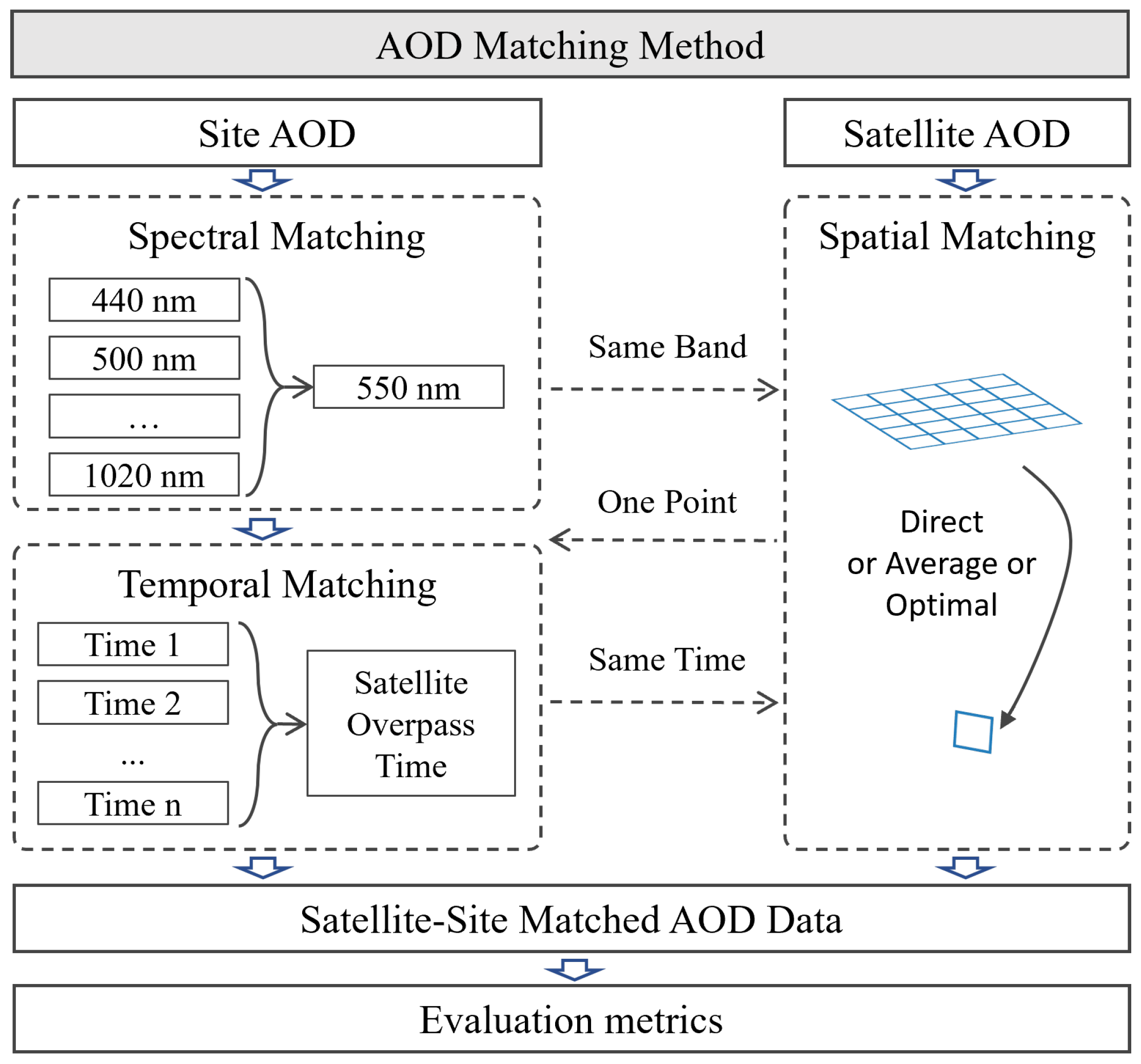
A specific pairing between a satellite-retrieved AOD and a site-measured AOD is referred to as a matchup. Due to differences in measurement methods between satellite and ground-based instruments, their products vary in spectral wavelength, time, and spatial coverage. Direct matching between site-measured and satellite-retrieved AOD is not feasible; thus, some processing is required [19,22,25], as shown in Figure 1.
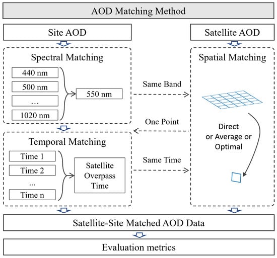
Figure 1.
AOD satellite-site matching framework.
In terms of spectral wavelength, AERONET does not provide measurements at 550 nm. Consequently, multi-wavelength AOD values from a single measurement were interpolated to 550 nm using a quadratic polynomial [35].
Regarding temporal aspects, a time discrepancy exists between ground-based measurements and the satellite overpass. Thus, AOD values at 550 nm were averaged from measurements taken within a 30-minute window before and after the satellite overpass [19].
Spatially, satellites provide snapshot measurements, whereas ground stations offer point measurements. To reconcile these differences, this study employs three methods:
- “Direct” Method: This method selects the satellite-derived AOD value from the pixel covering the ground station. Mathematically, the AOD value is determined aswhere represents the AOD value retrieved from the satellite at pixel i, and denotes the latitude and longitude coordinates of that pixel. The function computes the spatial distance between the satellite pixel and the ground station location . The index j corresponds to the object satellite pixel within the predefined spatial window W.
- “Average” Method: This common approach involves averaging AOD values within a spatial window centered on the ground station [19]. Mathematically, the AOD value is determined aswhere represents the AOD value retrieved from the satellite at pixel i, and denotes the total number of pixels within the spatial window W that contain valid retrievals.
- “Optimal” Method: This method, proposed in this study, selects the retrieved AOD value that exhibits the smallest absolute error relative to the ground-based measurement. Mathematically, the AOD value is determined aswhere represents the AOD value retrieved from the satellite at pixel i, and denotes the AOD measured by the ground station. The index j corresponds to the object satellite pixel within the spatial window W.
3.2. Differences of Three Spatial Matching Methods
Discrepancies between ground-based observations and satellite overpass times can make it difficult to locate the same aerosol layer in satellite imagery. Aerosols are transported by wind. Variations in wind speed and topography at different altitudes cause changes in aerosol distribution between the times of ground-based measurement and satellite overpass. This effect is more noticeable during high-wind events, making direct spatial matching less precise.
Despite the general assumption that aerosol distributions are spatially homogeneous over limited regions, fundamental differences in measurement techniques introduce significant retrieval uncertainties. Ground-based instruments derive AOD by measuring direct solar radiation, where the radiation traverses the atmospheric column only once. In contrast, satellite retrievals estimate AOD based on reflected radiance, requiring radiation to pass through the atmosphere twice. This distinction makes satellite-based AOD more susceptible to radiative perturbations, including subpixel cloud contamination, which can introduce retrieval biases. Consequently, satellite-retrieved AOD often exhibits enhanced spatial variability relative to actual atmospheric conditions.
The “direct” method assigns the satellite-derived AOD value from the pixel containing the ground station. However, it is particularly susceptible to temporal mismatches, as the retrieved aerosol may not correspond to the same air mass observed by the ground station. Additionally, this method cannot mitigate the impact of subpixel cloud contamination.
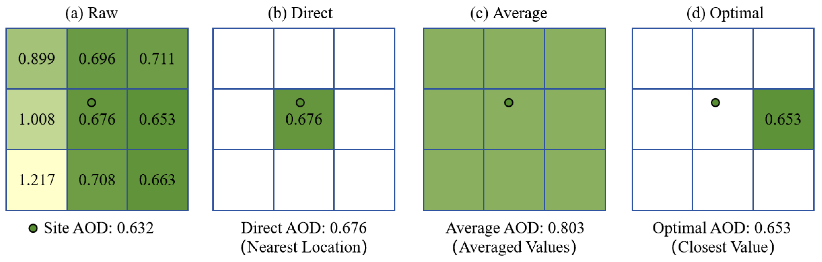
The “average” method reduces the impact of retrieval errors and localized anomalies with the assumption that aerosol concentrations vary smoothly over small spatial scales. Unlike the “direct” method, which relies on a single pixel, this approach averages AOD values from a surrounding spatial window, thereby mitigating errors arising from aerosol transport over time. However, in cases where subpixel clouds introduce outliers within the spatial window, the averaging process can lead to AOD values that deviate significantly from ground-based observations, as Figure 2 demonstrates.
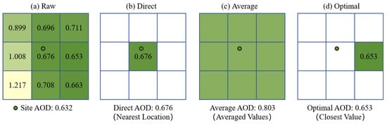
Figure 2.
Schematic diagram of three spatial matching methods. Squares represent pixels, while circles indicate ground sites. The values within the squares correspond to the AOD (QA = 3) retrievals from MOD(DT) for the granule “MOD04_L2.A2015219.1120.061.2017322082600.hdf”. The site AOD represents measurements from the AERONET Granada site. In panel (a), different colors denote variations in AOD values between the site measurement and pixel retrievals. Panels (b–d) illustrate the AOD values after applying different spatial matching methods. The closer color similarity between pixels and the site indicates a smaller retrieval–measurement difference.
The “optimal” method proposed in this study selects the satellite retrieval that minimizes the absolute error relative to the ground-based measurement. By prioritizing the retrieval with the smallest discrepancy, this approach mitigates the impact of subpixel cloud contamination, as the selected retrieval is less likely to be influenced by local radiative disturbances. Figure 2 presents the application of this method using real data, demonstrating its effectiveness in reducing the influence of outliers compared to the “average” method. However, two limitations remain:
- The selected pixel may not align with the true transport direction of aerosols, limiting the method’s physical interpretability and necessitating the assumption that aerosols are homogeneously distributed within the spatial window.
- This method is susceptible to retrieval algorithm biases. When the atmospheric conditions observed by the satellite differ significantly from those at the ground station, larger algorithmic errors can sometimes make the retrieved AOD appear closer to the ground-based measurement. As a result, the “optimal” method may select a retrieval that matches the observation numerically but does not accurately reflect the true aerosol conditions. For example, in MOD(DT), certain QA = 0 AOD values have been observed to align more closely with ground-based measurements than QA = 3 values, despite QA = 0 AOD retrievals potentially violating key algorithmic assumptions.
3.3. Selection of Window Size and Matching Constraints
For low-resolution products, the number of pixels within the spatial matching window is typically set to an odd number to ensure that the ground-based site is located at the central pixel and that spatial coverage is balanced in all directions. In this study, given that the analyzed datasets include products with a spatial resolution of 10 km, two primary window sizes were considered: 30 × 30 km2 and 50 × 50 km2. Both window sizes were evaluated, and the resulting distributions are presented in Table 2 and Table A1. Although the 50 × 50 km2 window produced better statistical performance than 30 × 30 km2 window, the overall conclusions remained consistent regardless of window size. The 30 × 30 km2 window is evenly divisible by the spatial resolutions of all products, which helps minimize discrepancies in spatial coverage during validation. Therefore, it was adopted for spatial matching in all three approaches used in this study. The total number of AOD values within the same spatial window varies across products due to differences in spatial resolution, ranging from as few as 9 pixels for 10 km products to as many as 900 pixels for 1 km products.
Table 2.
Validation results of matched pairs for the products using three matching methods.
To enhance the reliability of spatial collocation, we continue to assume that aerosol properties remain relatively uniform within a defined spatiotemporal window. To address temporal mismatches in both the “direct” and “optimal” methods, we average AOD values over a time window containing at least three valid observations. In the spatial domain, to prevent the “optimal” method from selecting retrievals that do not adhere to algorithmic assumptions, we still restrict the analysis to AOD values that meet the recommended quality assurance (QA) criteria or are flagged as “Best Quality” in the respective datasets. Although a higher number of high-quality pixels within the window expands the selection pool for the “optimal” method, imposing a threshold on the number of high-quality pixels may introduce artificial constraints, potentially leading to a favorable bias in the validation results rather than accurately reflecting real-world retrieval performance. AOD retrievals are independent of one another, and no such restriction is applied in the main text. Additionally, an alternative version, in which spatial matching is conducted only when the proportion of high-quality AOD retrievals within the spatial window exceeds 20%, is provided in Appendix A, Table A2. The application of this proportion-based quality threshold further enhances the performance of the “optimal” method.
3.4. Evaluation Metrics
Expected Level of Error (EE): EE, which combines absolute and relative error, is expressed as a confidence interval at approximately one standard deviation ( 67%). Greater consistency of data within this range when compared with ground measurements from AERONET indicates a more accurate AOD product [29]. For DT, the EE for AOD is defined as ±(0.05 + 20%), where QA = 3 [36], and for DB, it is ±(0.05 + 15%), where QA ≥ 2 [37,38]. This study employs the former, more stringent constraint for EE. The EE metric can be subdivided into the following three variables:
- =EE: Percentage of total data within the expected error range (±(0.05 + 15%)).
- >EE: Percentage of total data exceeding the expected value (+(0.05 + 15%)).
- <EE: Percentage of total data below the expected value (−(0.05 + 15%)).
Correlation Coefficient (CC): Pearson’s correlation coefficient quantifies the linear relationship between satellite retrievals and AERONET measurements, providing an indication of retrieval consistency.
Root Mean Square Error (RMSE): RMSE measures the overall deviation between retrievals and measurements, emphasizing larger discrepancies.
Relative Mean Bias (RMB): RMB assesses systematic over/underestimation trends.
Fractional Bias (FB): FB provides normalized error assessment robust to extreme values. It represents a measure of the bias that allows symmetric analysis of overestimation or underestimation by the model relative to observations [39].
The RMB and FB metrics are computed as
where N is the total number of pairs of modeled (M, i.e., MODIS) and observed (O, i.e., AERONET) values. The theoretical range of FB is from −200% and +200%, with 0 indicating the best value. RMB ranges from 0 to , and 1 is the best value.
In summary, the EE metric serves as a comprehensive evaluation criterion by integrating both absolute and relative errors. The proportion of retrievals falling within the EE range (=EE) is considered the primary indicator of algorithm performance. Additionally, CC, RMSE, RMB, and FB complement EE by capturing different aspects of retrieval accuracy, including systematic bias, overall error magnitude, and relative performance.
4. Results and Discussion
4.1. Overall Results Under Three Matching Methods
As the site measurements, satellite products, and QA selections are identical across all methods, spatial matching serves as the sole variable. Accordingly, the observed differences in performance metrics can be attributed exclusively to the spatial matching strategy. Table 2 presents the validation results for different spatial matching methods grouped by datasets.
In Table 2, the =EE percentage for the “optimal” method is consistently higher than the “average” and “direct” methods across all datasets, with an improvement range of 10% to 30%. Substantial reductions are also observed in both RMB and FB. These results suggest that retrieval values near the validation sites are generally more accurate. Some high-QA points, however, are influenced by subpixel clouds or shadows, making them less optimal. In contrast, the surrounding points, which are unaffected by these factors, provide a more accurate AOD estimate.
It is noteworthy that even under the “optimal” spatial matching strategy, the >EE results consistently exceed the <EE results for each product. This indicates that, among the outliers, overestimations are more frequent than underestimations. Moreover, the RMB is consistently positive across all datasets, further confirming a systematic tendency toward AOD overestimation. This positive bias may result from several contributing factors:
- First, although the “optimal” method aims to select retrievals spatially closest to the AERONET site, it cannot fully eliminate the influence of subpixel clouds or cloud shadows. Residual thin clouds or elevated humidity levels may be misclassified as aerosol signals, leading to inflated AOD estimates. This effect is particularly pronounced in regions with frequent convective activity or in humid seasons, where cloud contamination is more difficult to detect.
- Second, most aerosol retrieval algorithms favor pixels with lower surface reflectance, as these conditions enhance the aerosol signal-to-noise ratio. However, this selection preference may introduce a bias: by preferentially using pixels with darker surfaces, the algorithm may adopt surface reflectance values that are lower than the actual conditions at the time of observation. This can lead to a systematic overestimation of aerosol loading. Additionally, in heterogeneous or dynamic surface environments, static surface reflectance databases may not accurately represent current surface conditions, further contributing to retrieval errors.
In both the “direct” and “average” method validations, the AOD products from the DT algorithm demonstrated the lowest accuracy among the three algorithms (DT, DB, MAIAC), with a potential accuracy difference of 10-20% compared to the others. However, in the “optimal” method validation, the accuracy of the MODIS DT algorithm improved, approaching that of the DB algorithm. This indicates that the accuracy difference between the DB and DT algorithms is minimal at the algorithm level. Nevertheless, the significant discrepancy in product accuracy highlights substantial room for improvement in the DT algorithm’s quality control. For both the NOAA and SNPP products, the DB algorithm outperformed the DT algorithm by 10-17% in accuracy when the optimal comparison method was applied. This suggests that, in terms of accuracy, the DB algorithm on VIIRS has undergone more significant improvements after transitioning to operational use compared to the DT algorithm.
Interestingly, the 3 km resolution AOD product generated by the DT algorithm exhibited the greatest accuracy variation among the three validation methods. The “optimal” method improved validation accuracy by 25% to 30%, exceeding the accuracy of both the 10 km DT and DB algorithms. This result highlights two key observations:
- First, the DT algorithm is highly sensitive to dark target pixels, showing particularly high accuracy for pixels that meet the dark target criteria. From the perspective of optimal pixel selection, accuracy improves significantly when a sufficient number of pixels meet the dark target criteria.
- Second, as the resolution increases to 3 km, the higher pixel resolution and purer dark target signals lead to improved retrieval accuracy. However, for pixels that do not fully meet the criteria, the accuracy is more heavily impacted, resulting in greater uncertainty.
The DTB product, combined from the DT and DB products, primarily expanded the coverage but did not lead to a significant improvement in accuracy. The results show that, in the “direct” method, the =EE percentage of the DTB product is only marginally higher than that of the DT product and 6% lower than the DB product from the same sensor. The quality control method applied in the DT product is more lenient when selecting high-quality points, which results in a larger average deviation between retrieval values and measurements. This process likely introduced additional biases during synthesis, which may have counteracted the strengths of the DB algorithm, leading to a reduction in overall accuracy. Therefore, in terms of accuracy, the DTB product did not meet expectations.
In the “optimal” results, the MAIAC product performs the best. MOD(MAIAC) achieves the highest percentage of =EE at 94%, with MYD(MAIAC) closely following at 93.5%. The high accuracy of the MAIAC product can be attributed to two main factors. First, it utilizes time-series data, assuming that surface reflectance changes are minimal over short periods. Under this assumption, the algorithm identifies the clearest day within a time series, using a series of operations to obtain accurate Bidirectional Reflectance Factor (BRF) values, which are then used to retrieve the AOD for the target time [17]. During this process, the design of the time-series filter and the minimization of the objective function effectively filter out many undetected cloud and cloud shadow pixels, thus reducing errors caused by these factors. Second, the MAIAC algorithm retrieves AOD at a 1 km resolution. The higher spatial resolution of the pixels allows for purer land surface characteristics, which are more consistent with the algorithm’s assumptions compared to lower-resolution pixels. As a result, some pixels achieve higher AOD accuracy in the “optimal” method.
In both the “average” and “optimal” methods, products with higher resolution typically yield more matching pairs, primarily due to the purity of their pixels. In low-resolution products, certain pixel areas may be assigned lower QA flags due to cloud cover. However, in higher-resolution products, the same area is subdivided into smaller pixels, where cloud-free pixels are assigned higher QA flags, thus increasing the number of matching pairs. Additionally, as the successor to MODIS, the VIIRS sensor has a similar revisit cycle but offers a wider swath and higher spatial resolution. These features enable the VIIRS sensor to provide more matching data. When prioritizing the number of matches, both the VIIRS DB product and the MODIS MAIAC product demonstrate distinct advantages in terms of matching pairs and retrieval accuracy, making them highly recommended for use.
Table 3 presents validation results across different EE ranges to further support the previous conclusions. Four EE ranges are provided in the table. Here, “max (0.03;10%)” refers to selecting the larger value between absolute error and relative error as the EE range, which is narrower than the “(0.03 + 10%)” range. The results show that, although the EE percentage decreases across all products as the envelope range narrows, the previous conclusions remain valid. Additionally, the DT products, particularly those from VIIRS, perform poorly across different EE ranges. In contrast, the MOD(MAIAC) dataset consistently achieves the highest percentage under the “optimal” method, while the SNPP(DB) dataset performs best under the “direct” and “average” methods.
Table 3.
Validation results across different EE ranges for AOD products.
4.2. Impact of Land Cover and Seasonal Variability on Retrieval Accuracy
4.2.1. Land Cover Variability
Figure 3 presents the validation results of various satellite AOD products, expressed in terms of the expected error (EE) metric, under different spatial collocation strategies and land cover types. Although the “optimal” method generally improves validation accuracy compared to the “direct” and “average” methods, retrievals still exhibit a systematic overestimation bias. This bias is particularly pronounced over bareland surfaces and for the DT product.
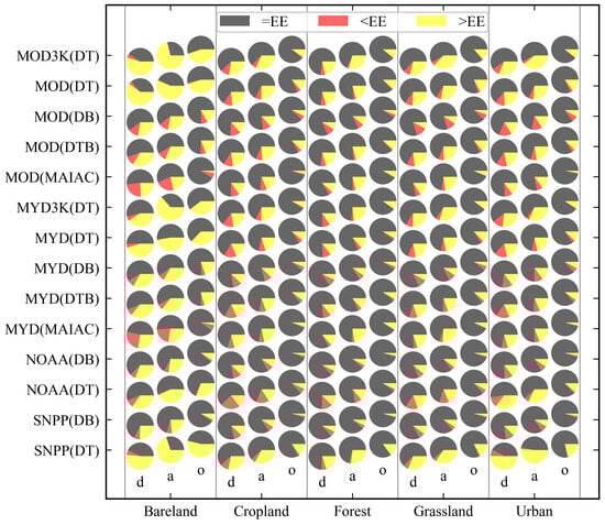
Figure 3.
Comparison of AOD retrieval accuracy across different land cover types using various satellite aerosol products. Each pie chart represents the proportion of retrievals falling within (=EE, gray), above (>EE, yellow), or below (<EE, red) the expected error range (EE). The x-axis categorizes IGBP land cover types from the MCD12C1 product, with three spatial matching methods applied: direct (d), average (a), and optimal (o).
Among the three algorithms, the MAIAC product shows the best performance over bareland regions under the “optimal” method, followed by DB, and DT performs the worst. The DT algorithm’s poor performance mainly results from its invalid assumptions over bright surfaces. Compared to the “average” method, MAIAC shows an exaggerated improvement under the “optimal” method, suggesting that the MAIAC product exhibits large variance and uncertainty over bare surfaces. Moreover, the underestimation bias of MAIAC is more evident in bareland areas than in other products. In such regions, high surface reflectance reduces the aerosol signal strength. Moreover, significant temporal variations in reflectance—caused by factors such as precipitation, wind-blown dust, or soil moisture—may cause the temporal filtering mechanism of MAIAC to misinterpret low AOD values as valid retrievals, thereby introducing a systematic underestimation. Furthermore, the dominance of surface-reflected radiance in the satellite signal complicates the extraction of the aerosol scattering component. To minimize retrieval errors arising from surface reflectance uncertainty, the MAIAC algorithm may be biased toward lower AOD values. Improving the adaptability of AOD retrieval algorithms over bareland remains a key challenge for future product development.
Among all evaluated products, the SNPP (DT) product exhibits the poorest performance across land cover types. As shown in Figure 3, SNPP (DT) yields the lowest proportion of retrievals within the EE envelope and the highest proportion exceeding the EE threshold for all land types, indicating large retrieval errors. These findings further support the view that the migration of the DT algorithm to the SNPP platform has not been successful.
4.2.2. Seasonal Variability
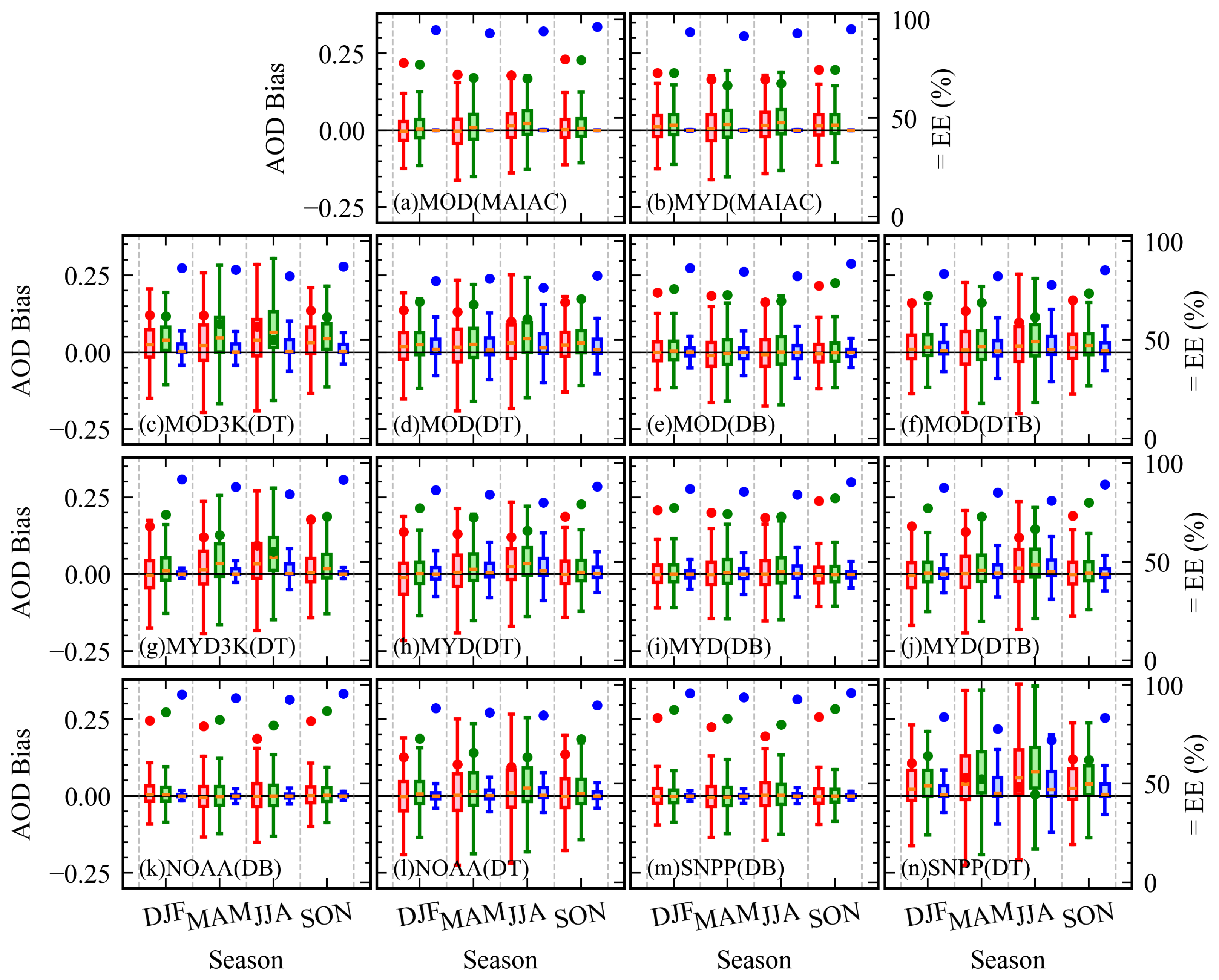
Different aerosol optical depth (AOD) products exhibit notable seasonal variability; however, the seasonal patterns observed at individual sites vary by region. As shown in Figure 4, the results represent the overall retrieval bias across global AERONET sites. AOD biases tend to be smaller and more stable during autumn (SON) and winter (DJF), whereas larger biases and greater variability are observed in spring (MAM) and summer (JJA). This pattern can be attributed to stronger evaporation during summer, which induces rapid changes in atmospheric humidity and wind speed. These dynamic conditions, including intensified cloud formation, enhanced hygroscopic growth of aerosols, and rapid changes in surface reflectance, collectively increase the susceptibility of satellite retrieval algorithms to systematic biases.
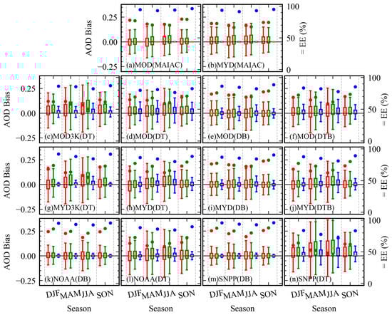
Figure 4.
Seasonal variations in AOD bias for different satellite aerosol products and retrieval methods. Red, green, and blue represent the direct, average, and optimal spatial matching methods, respectively. The box plots illustrate the AOD bias distributions across four seasons: DJF (December–February), MAM (March–May), JJA (June–August), and SON (September–November). The right y-axis denotes the percentage of retrievals falling within the expected error (EE), with circular markers for each method.
Among the spatial matching approaches, the optimal method effectively reduces AOD bias and improves the fraction of retrievals within the expected error (EE). Nevertheless, it does not eliminate the underlying seasonal trend, which primarily reflects algorithmic limitations in adapting to rapidly evolving atmospheric and surface conditions.
4.3. Comparison of DB and DT Products at Site Level
To provide a more detailed and intuitive comparison of the differences between the three methods, a statistical analysis was conducted at the site level. For simplicity in presentation and description, only the DT and DB algorithm products from the same sensor were compared. These products share the same satellite overpass time, ensuring that the observed differences can primarily be attributed to the retrieval algorithms used, thereby strengthening the reliability of the comparison.
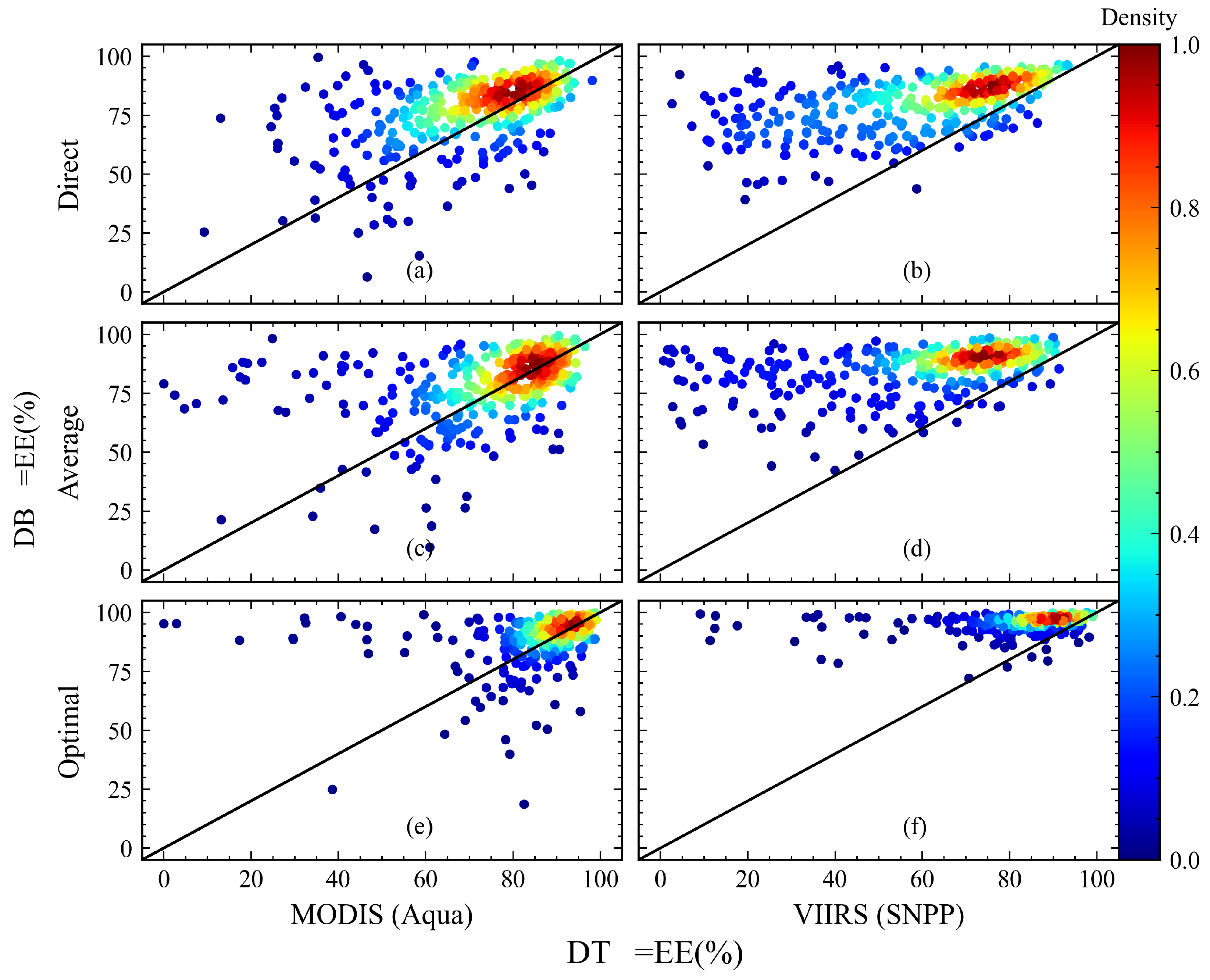
To assess the impact of the three matching methods on the results at different AERONET sites, a comparison of the accuracy between the DT and DB datasets of the same product was plotted (Figure 5). For the MODIS dataset, the higher-accuracy MYD dataset was selected, while the longer-duration SNPP dataset was used for the VIIRS data. Thus, the statistical analysis utilized the following datasets: MYD(DT), MYD(DB), SNPP(DT), and SNPP(DB). To improve statistical reliability, sites with fewer than 50 AERONET matchups were excluded, resulting in 335 sites used for analysis.
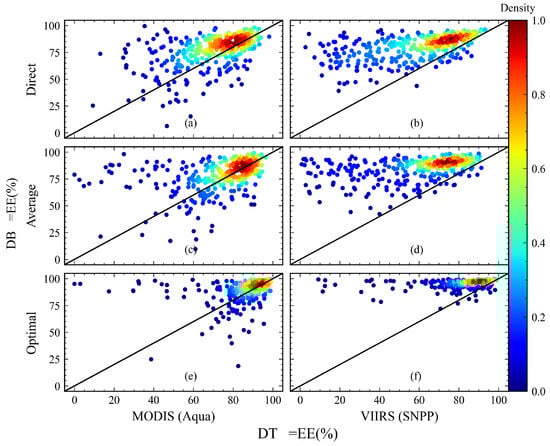
Figure 5.
Comparison of =EE between DT and DB AOD products for MODIS (Aqua) and VIIRS (SNPP) under different spatial matching methods. The color scale indicates the density of data points, with red representing higher densities. The diagonal black line represents the 1:1 reference line, where DT and DB products have equal EE percentages.
Figure 5 clearly demonstrates that the “optimal” method significantly enhances validation accuracy across most sites. In a 1:1 scatter plot, points positioned closer to the top indicate better performance in the vertical-axis metric, while those near the right end reflect better performance in the horizontal-axis metric. Under the optimal method, the AOD retrievals for MYD products exhibit a more pronounced concentration toward the upper-right region of the plot compared to other spatial matching methods. This suggests that both DT and DB products experience substantial improvements in the =EE metric, with the majority of sites showing enhanced accuracy.
As shown in Figure 5, the majority of scatter points lie above the 1:1 reference line, indicating that the DB algorithm generally provides more accurate AOD retrievals than the DT algorithm. The DB algorithm utilizes additional information from the deep blue spectral band, which is less sensitive to surface reflectance variations and, therefore, more effective over bright surfaces, such as arid or semi-arid regions. Its broader applicability to various surface types further contributes to its superior performance at a greater number of sites. For the SNPP product, the outperformance of DB over DT at nearly all sites suggests a potential systematic bias in the implementation of the DT algorithm. To further examine this issue, a detailed comparative analysis is carried out at two representative sites.
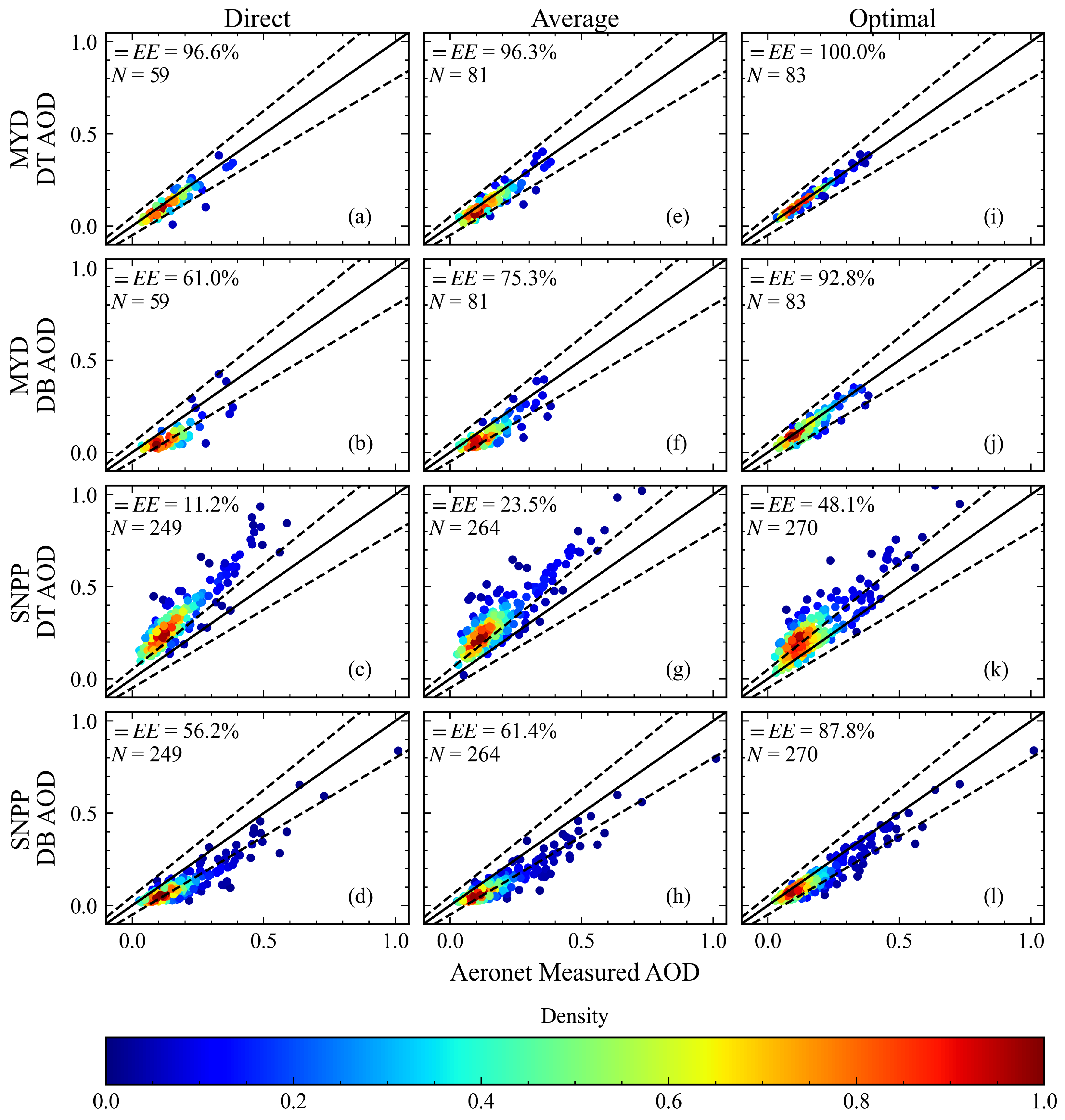
Figure 6 and Figure 7 present the results of three spatial matching methods at two representative sites: Mexico City and São Paulo. Both sites are located in regions where the MODIS DT algorithm performs optimally, generally yielding higher retrieval accuracy than the DB algorithm. In densely vegetated urban areas, the DT algorithm can identify a sufficient number of “dark” targets, enabling more accurate retrievals. In contrast, the DB algorithm is more susceptible to interference from “bright” pixels in these regions. Among the three evaluated methods, the “optimal” approach consistently improves accuracy metrics across different products. However, not all products achieve the expected accuracy after applying the “optimal” method, particularly when the retrieval algorithm itself is not well-suited to the region.
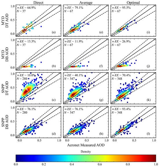
Figure 6.
Validation charts of DT and DB products for Mexico City site.
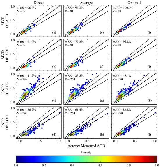
Figure 7.
Validation charts of DT and DB products for Sao Paulo site.
At the Mexico City site, the performance of the MODIS DB product is affected by persistent pollution [18], whereas the VIIRS product demonstrates significant improvement following the implementation of an updated smoke algorithm. As shown in the figures, inherent limitations in the MODIS DB algorithm persist even when the “optimal” method is applied, resulting in relatively low accuracy. Compared to the “average” method, the “optimal” approach effectively minimizes residual cloud contamination and reduces the influence of outliers, resulting in a tighter scatter distribution within the expected error envelope. The validation images generated by the “optimal” method are clearer, facilitating the identification of potential issues. Similarly, at the São Paulo site, the VIIRS DT algorithm does not achieve the desired accuracy even after applying the “optimal” method, suggesting that further refinement of the algorithm is necessary.
The site-level analysis highlights differences among the three spatial matching methods while also yielding additional insights. Although the DB product generally exhibits higher accuracy than the DT product in most regions, site-specific comparisons indicate that each algorithm has distinct advantages, and the DB product cannot entirely replace the DT product. As the first global aerosol retrieval algorithm implemented for MODIS, the DT algorithm inevitably involves a trade-off between retrieval quality and spatial coverage. To maximize its advantages, refining the quality control mechanism is recommended to enhance product reliability.
Combining the DT and DB products into a unified DTB product presents a promising strategy. Currently, the DTB product determines the applicability of DT or DB retrievals based on NDVI and utilizes QA values for synthesis in transition regions. However, this approach remains relatively simplistic and has not led to a significant improvement in overall accuracy [1]. Based on the above analysis, the following strategies could enhance the accuracy of the DTB product:
- Optimization of surface feature selection: Existing site data can be leveraged to identify the most suitable surface characteristics for the DT algorithm. A global mask could then be developed to ensure that the DT algorithm is applied exclusively in these regions.
- Improved resolution adaptation: Given the strict applicability assumptions of the DT algorithm, employing it at higher resolutions would allow for the selection of clearer pixels that meet retrieval criteria, thereby enhancing overall accuracy.
5. Conclusions
This study systematically validated MODIS and VIIRS AOD products against AERONET ground observations using three spatial matching methods: “direct”, “average”, and “optimal”. The results indicate that the “optimal” method significantly reduces errors associated with quality control algorithms but does not eliminate the inherent retrieval biases of the algorithms themselves. Consequently, the “optimal” method provides a more accurate assessment of retrieval algorithm performance.
It is important to note that the “optimal” method represents the upper bound of retrieval accuracy and, therefore, cannot entirely replace the “average” method. Instead, it should be considered a complementary approach. As a post-processing validation method, the “optimal” method is site-dependent and cannot be directly integrated into the retrieval process. However, it can be applied to filter existing datasets, thereby generating high-quality sample sets, which can be used as optimized inputs for deep learning models and other advanced analytical approaches.
In summary, this study highlights the unique advantages of the “optimal” spatial matching method in more accurately reflecting the intrinsic retrieval accuracy of AOD algorithms. These findings underscore the importance of enhancing quality control mechanisms to improve AOD product accuracy and reliability in satellite-based aerosol monitoring. For data users, these insights facilitate more optimized dataset applications, while for algorithm developers, they provide clearer pathways for algorithmic enhancement.
Author Contributions
Conceptualization, B.D.; methodology, B.D., B.Z., H.C. and S.W.; validation, B.D.; data curation, B.D., S.W. and H.C.; resources, B.Z., J.W., A.Y. and Q.L.; writing–original draft preparation, B.D.; writing–review and editing B.D., B.Z., H.C., Y.Q., X.W., Q.L., H.Z. and J.J.; funding acquisition, B.Z. and Q.L. All authors have read and agreed to the published version of the manuscript.
Funding
This research was supported by the National Key Research and Development Program of China (No. 2024YFF1306102).
Data Availability Statement
The datasets used in this study are publicly available. These data were derived from the following resources available in the public domain: MODIS and VIIRS data at https://search.earthdata.nasa.gov (accessed on 26 October 2024); AERONET data at https://aeronet.gsfc.nasa.gov/cgi-bin/webtool_aod_v3 (accessed on 13 May 2024).
Acknowledgments
We thank the reviewers for their insightful comments and suggestions, which helped improve our manuscript.
Conflicts of Interest
The Author Jingxiong Jiang was employed by the Space Star Technology Co., Ltd. The remaining authors declare that the research was conducted in the absence of any commercial or financial relationships that could be construed as a potential conflict of interest. The authors declare no conflicts of interest.
Appendix A. Validation Results
Table A1.
Validation results of three methods with at least one high-quality pixel (50 × 50 km2 window).
Table A1.
Validation results of three methods with at least one high-quality pixel (50 × 50 km2 window).
| Alias | Method | >EE(%) | =EE(%) | <EE(%) | R2 | RMSE | CC | RMB | FB(%) | Pairs | Sites |
|---|---|---|---|---|---|---|---|---|---|---|---|
| MOD3K (DT) | direct | 29.53 | 62.09 | 8.38 | 0.559 | 0.156 | 0.83 | 1.21 | 18.01 | 111,304 | 814 |
| average | 37.1 | 59.11 | 3.79 | 0.638 | 0.129 | 0.874 | 1.365 | 36.78 | 264,711 | 854 | |
| optimal | 10.08 | 89.45 | 0.48 | 0.9 | 0.067 | 0.955 | 1.117 | 14.6 | 270,330 | 854 | |
| MOD (DT) | direct | 25.6 | 64.73 | 9.67 | 0.586 | 0.147 | 0.826 | 1.142 | 12.68 | 139,319 | 821 |
| average | 28.44 | 66.34 | 5.22 | 0.726 | 0.115 | 0.891 | 1.23 | 24.11 | 212,138 | 848 | |
| optimal | 12.83 | 85.4 | 1.77 | 0.875 | 0.077 | 0.943 | 1.116 | 14.75 | 217,053 | 848 | |
| MOD (DB) | direct | 12.89 | 73.54 | 13.57 | 0.65 | 0.132 | 0.839 | 0.966 | −14.26 | 182,715 | 795 |
| average | 14.03 | 74.13 | 11.84 | 0.729 | 0.116 | 0.874 | 1.004 | −5.79 | 226,706 | 808 | |
| optimal | 5.5 | 89.39 | 5.11 | 0.873 | 0.08 | 0.938 | 0.988 | −3.29 | 226,706 | 808 | |
| MOD (DTB) | direct | 22.58 | 66.18 | 11.24 | 0.578 | 0.145 | 0.82 | 1.102 | 4.73 | 179,540 | 837 |
| average | 23.68 | 69.48 | 6.83 | 0.723 | 0.115 | 0.885 | 1.172 | 15.59 | 244,392 | 859 | |
| optimal | 9.54 | 88.09 | 2.37 | 0.881 | 0.075 | 0.944 | 1.076 | 8.09 | 249,095 | 859 | |
| MOD (MAIAC) | direct | 16.19 | 74.81 | 9.0 | 0.754 | 0.095 | 0.872 | 1.028 | 6.82 | 232,087 | 829 |
| average | 18.34 | 74.32 | 7.34 | 0.75 | 0.1 | 0.868 | 1.072 | 16.05 | 310,077 | 760 | |
| optimal | 3.02 | 95.92 | 1.06 | 0.943 | 0.047 | 0.971 | 1.01 | 3.54 | 309,173 | 760 | |
| MYD3K (DT) | direct | 24.87 | 64.55 | 10.58 | 0.438 | 0.175 | 0.749 | 1.101 | 6.0 | 104,923 | 824 |
| average | 29.47 | 66.04 | 4.49 | 0.658 | 0.125 | 0.871 | 1.268 | 22.33 | 245,354 | 850 | |
| optimal | 8.09 | 91.32 | 0.59 | 0.899 | 0.067 | 0.953 | 1.089 | 9.87 | 254,751 | 850 | |
| MYD (DT) | direct | 21.53 | 66.29 | 12.18 | 0.435 | 0.176 | 0.728 | 1.03 | 0.55 | 121,026 | 824 |
| average | 21.63 | 72.41 | 5.95 | 0.735 | 0.112 | 0.887 | 1.15 | 10.77 | 190,472 | 839 | |
| optimal | 9.69 | 88.16 | 2.14 | 0.87 | 0.078 | 0.938 | 1.076 | 7.12 | 197,096 | 839 | |
| MYD (DB) | direct | 12.87 | 76.19 | 10.94 | 0.653 | 0.13 | 0.84 | 0.997 | −9.17 | 155,875 | 775 |
| average | 13.99 | 76.26 | 9.75 | 0.744 | 0.113 | 0.881 | 1.026 | −1.98 | 201,296 | 797 | |
| optimal | 5.58 | 90.26 | 4.15 | 0.879 | 0.078 | 0.94 | 1.002 | −1.24 | 201,295 | 797 | |
| MYD (DTB) | direct | 19.94 | 67.49 | 12.57 | 0.459 | 0.167 | 0.744 | 1.025 | −2.78 | 157,158 | 839 |
| average | 19.14 | 74.01 | 6.85 | 0.734 | 0.112 | 0.886 | 1.12 | 6.34 | 222,677 | 850 | |
| optimal | 7.74 | 89.89 | 2.37 | 0.877 | 0.075 | 0.942 | 1.054 | 3.43 | 229,127 | 850 | |
| MYD (MAIAC) | direct | 21.06 | 71.28 | 7.66 | 0.758 | 0.097 | 0.875 | 1.089 | 17.43 | 251,899 | 840 |
| average | 22.2 | 71.15 | 6.65 | 0.748 | 0.102 | 0.87 | 1.12 | 24.21 | 320,728 | 765 | |
| optimal | 3.56 | 95.29 | 1.15 | 0.939 | 0.05 | 0.969 | 1.017 | 5.02 | 319,633 | 765 | |
| NOAA (DB) | direct | 13.1 | 78.13 | 8.77 | 0.66 | 0.133 | 0.837 | 1.02 | −2.41 | 115,751 | 561 |
| average | 10.5 | 82.98 | 6.51 | 0.822 | 0.091 | 0.913 | 1.019 | 1.13 | 151,796 | 562 | |
| optimal | 3.0 | 95.68 | 1.32 | 0.947 | 0.05 | 0.973 | 1.01 | 2.04 | 151,796 | 562 | |
| NOAA (DT) | direct | 24.31 | 60.87 | 14.81 | 0.208 | 0.199 | 0.67 | 1.09 | −2.37 | 100,700 | 581 |
| average | 19.87 | 70.58 | 9.54 | 0.664 | 0.124 | 0.862 | 1.111 | 1.12 | 152,090 | 584 | |
| optimal | 6.04 | 91.92 | 2.04 | 0.883 | 0.071 | 0.944 | 1.041 | 1.7 | 165,633 | 587 | |
| SNPP (DB) | direct | 12.1 | 79.32 | 8.58 | 0.684 | 0.126 | 0.847 | 1.01 | −2.92 | 239,122 | 800 |
| average | 9.63 | 83.51 | 6.86 | 0.832 | 0.089 | 0.917 | 1.003 | 0.03 | 313,791 | 814 | |
| optimal | 2.65 | 95.91 | 1.45 | 0.947 | 0.05 | 0.973 | 1.004 | 1.8 | 313,791 | 814 | |
| SNPP (DT) | direct | 37.2 | 55.3 | 7.51 | −0.027 | 0.226 | 0.7 | 1.395 | 26.09 | 203,907 | 834 |
| average | 38.44 | 58.03 | 3.53 | 0.455 | 0.157 | 0.861 | 1.435 | 34.39 | 325,935 | 850 | |
| optimal | 13.03 | 86.27 | 0.69 | 0.805 | 0.093 | 0.926 | 1.167 | 15.35 | 336,799 | 850 |
Table A2.
Validation results of three methods with a 20% high-quality pixel constraint (30 × 30 km2 window).
Table A2.
Validation results of three methods with a 20% high-quality pixel constraint (30 × 30 km2 window).
| Alias | Method | >EE(%) | =EE(%) | <EE(%) | R2 | RMSE | CC | RMB | FB(%) | Pairs | Sites |
|---|---|---|---|---|---|---|---|---|---|---|---|
| MOD3K (DT) | direct | 29.53 | 62.09 | 8.38 | 0.559 | 0.156 | 0.83 | 1.21 | 18.01 | 111,304 | 814 |
| average | 27.59 | 68.09 | 4.33 | 0.756 | 0.107 | 0.913 | 1.233 | 23.36 | 157,466 | 799 | |
| optimal | 2.67 | 96.86 | 0.46 | 0.972 | 0.036 | 0.987 | 1.032 | 5.19 | 162,100 | 799 | |
| MOD (DT) | direct | 25.6 | 64.73 | 9.67 | 0.586 | 0.147 | 0.826 | 1.142 | 12.68 | 139,319 | 821 |
| average | 24.86 | 69.43 | 5.71 | 0.749 | 0.111 | 0.904 | 1.188 | 17.28 | 153,143 | 810 | |
| optimal | 12.04 | 85.29 | 2.67 | 0.878 | 0.077 | 0.946 | 1.095 | 10.36 | 156,800 | 811 | |
| MOD (DB) | direct | 12.89 | 73.54 | 13.57 | 0.65 | 0.132 | 0.839 | 0.966 | −14.26 | 182,715 | 795 |
| average | 12.9 | 75.67 | 11.43 | 0.756 | 0.11 | 0.888 | 0.994 | −7.54 | 187,093 | 782 | |
| optimal | 5.75 | 87.9 | 6.35 | 0.868 | 0.081 | 0.936 | 0.973 | −6.5 | 187,093 | 782 | |
| MOD (DTB) | direct | 22.58 | 66.18 | 11.24 | 0.578 | 0.145 | 0.82 | 1.102 | 4.73 | 179,540 | 837 |
| average | 21.35 | 71.11 | 7.54 | 0.735 | 0.113 | 0.893 | 1.141 | 9.91 | 190,897 | 836 | |
| optimal | 9.81 | 86.3 | 3.89 | 0.867 | 0.079 | 0.939 | 1.06 | 3.89 | 194,512 | 837 | |
| MOD (MAIAC) | direct | 16.19 | 74.81 | 9.0 | 0.754 | 0.095 | 0.872 | 1.028 | 6.82 | 232,087 | 829 |
| average | 12.46 | 80.09 | 7.45 | 0.814 | 0.081 | 0.902 | 1.011 | 9.45 | 270,861 | 798 | |
| optimal | 0.68 | 98.16 | 1.16 | 0.97 | 0.032 | 0.986 | 0.985 | 1.08 | 270,450 | 798 | |
| MYD3K (DT) | direct | 24.87 | 64.55 | 10.58 | 0.438 | 0.175 | 0.749 | 1.101 | 6.0 | 104,923 | 824 |
| average | 20.09 | 75.08 | 4.83 | 0.772 | 0.1 | 0.912 | 1.151 | 8.69 | 141,317 | 805 | |
| optimal | 1.5 | 98.06 | 0.44 | 0.975 | 0.033 | 0.988 | 1.016 | 1.35 | 148,716 | 805 | |
| MYD (DT) | direct | 21.53 | 66.29 | 12.18 | 0.435 | 0.176 | 0.728 | 1.03 | 0.55 | 121,026 | 824 |
| average | 19.35 | 74.69 | 5.96 | 0.768 | 0.104 | 0.906 | 1.123 | 5.27 | 132,668 | 806 | |
| optimal | 8.68 | 88.5 | 2.83 | 0.889 | 0.071 | 0.949 | 1.056 | 2.41 | 137,172 | 806 | |
| MYD (DB) | direct | 12.87 | 76.19 | 10.94 | 0.653 | 0.13 | 0.84 | 0.997 | −9.17 | 155,875 | 775 |
| average | 12.65 | 78.08 | 9.27 | 0.773 | 0.105 | 0.896 | 1.018 | −3.47 | 160,047 | 759 | |
| optimal | 5.58 | 89.5 | 4.92 | 0.88 | 0.076 | 0.942 | 0.991 | −3.74 | 160,046 | 759 | |
| MYD (DTB) | direct | 19.94 | 67.49 | 12.57 | 0.459 | 0.167 | 0.744 | 1.025 | −2.78 | 157,158 | 839 |
| average | 17.82 | 75.13 | 7.04 | 0.753 | 0.107 | 0.898 | 1.103 | 2.44 | 167,487 | 829 | |
| optimal | 7.72 | 88.83 | 3.44 | 0.879 | 0.074 | 0.944 | 1.04 | −0.5 | 171,837 | 829 | |
| MYD (MAIAC) | direct | 21.06 | 71.28 | 7.66 | 0.758 | 0.097 | 0.875 | 1.089 | 17.43 | 251,899 | 840 |
| average | 17.57 | 75.78 | 6.65 | 0.808 | 0.085 | 0.9 | 1.069 | 19.44 | 287,430 | 805 | |
| optimal | 1.31 | 97.4 | 1.29 | 0.964 | 0.037 | 0.983 | 0.992 | 3.33 | 286,755 | 805 | |
| NOAA (DB) | direct | 13.1 | 78.13 | 8.77 | 0.66 | 0.133 | 0.837 | 1.02 | −2.41 | 115,751 | 561 |
| average | 8.77 | 85.18 | 6.05 | 0.851 | 0.085 | 0.928 | 1.007 | −0.67 | 115,163 | 538 | |
| optimal | 1.57 | 97.04 | 1.39 | 0.957 | 0.045 | 0.979 | 0.991 | −0.64 | 115,163 | 538 | |
| NOAA (DT) | direct | 24.31 | 60.87 | 14.81 | 0.208 | 0.199 | 0.67 | 1.09 | −2.37 | 100,700 | 581 |
| average | 19.18 | 71.69 | 9.13 | 0.658 | 0.122 | 0.872 | 1.112 | −1.41 | 107,791 | 574 | |
| optimal | 3.76 | 92.99 | 3.25 | 0.9 | 0.064 | 0.953 | 1.001 | −4.77 | 116,924 | 577 | |
| SNPP (DB) | direct | 12.1 | 79.32 | 8.58 | 0.684 | 0.126 | 0.847 | 1.01 | −2.92 | 239,122 | 800 |
| average | 7.83 | 85.92 | 6.25 | 0.863 | 0.081 | 0.933 | 0.991 | −1.52 | 239,053 | 769 | |
| optimal | 1.3 | 97.23 | 1.47 | 0.961 | 0.043 | 0.98 | 0.986 | −0.77 | 239,053 | 769 | |
| SNPP (DT) | direct | 37.2 | 55.3 | 7.51 | −0.027 | 0.226 | 0.7 | 1.395 | 26.09 | 203,907 | 834 |
| average | 36.49 | 60.32 | 3.19 | 0.439 | 0.154 | 0.874 | 1.429 | 31.31 | 233,619 | 820 | |
| optimal | 11.26 | 87.75 | 0.99 | 0.842 | 0.081 | 0.944 | 1.145 | 12.21 | 241,513 | 820 |
References
- Bilal, M.; Nichol, J.E.; Wang, L. New customized methods for improvement of the MODIS C6 Dark Target and Deep Blue merged aerosol product. Remote Sens. Environ. 2017, 197, 115–124. [Google Scholar]
- Haywood, J.; Boucher, O. Estimates of the direct and indirect radiative forcing due to tropospheric aerosols: A review. Rev. Geophys. 2000, 38, 513–543. [Google Scholar]
- Ramanathan, V.; Crutzen, P.J.; Kiehl, J.; Rosenfeld, D. Aerosols, climate, and the hydrological cycle. Science 2001, 294, 2119–2124. [Google Scholar] [CrossRef]
- Ramanathan, V.; Carmichael, G. Global and regional climate changes due to black carbon. Nat. Geosci. 2008, 1, 221–227. [Google Scholar]
- Brunekreef, B.; Holgate, S.T. Air pollution and health. Lancet 2002, 360, 1233–1242. [Google Scholar] [CrossRef]
- Pöschl, U. Atmospheric aerosols: Composition, transformation, climate and health effects. Angew. Chem. Int. Ed. 2005, 44, 7520–7540. [Google Scholar] [CrossRef]
- Dubovik, O.; Holben, B.; Eck, T.F.; Smirnov, A.; Kaufman, Y.J.; King, M.D.; Tanré, D.; Slutsker, I. Variability of absorption and optical properties of key aerosol types observed in worldwide locations. J. Atmos. Sci. 2002, 59, 590–608. [Google Scholar]
- Kaufman, Y.J.; Tanré, D.; Boucher, O. A satellite view of aerosols in the climate system. Nature 2002, 419, 215–223. [Google Scholar] [CrossRef]
- Kassianov, E.; Cromwell, E.; Monroe, J.; Riihimaki, L.D.; Flynn, C.; Barnard, J.; Michalsky, J.J.; Hodges, G.; Shi, Y.; Comstock, J.M. Harmonized and high-quality datasets of aerosol optical depth at a US continental site, 1997–2018. Sci. Data 2021, 8, 82. [Google Scholar]
- Papachristopoulou, K.; Raptis, I.P.; Gkikas, A.; Fountoulakis, I.; Masoom, A.; Kazadzis, S. Aerosol optical depth regime over megacities of the world. Atmos. Chem. Phys. 2022, 22, 15703–15727. [Google Scholar]
- Wang, Y.; Wang, J.; Levy, R.C.; Shi, Y.R.; Mattoo, S.; Reid, J.S. First retrieval of AOD at fine resolution over shallow and turbid coastal waters from MODIS. Geophys. Res. Lett. 2021, 48, e2021GL094344. [Google Scholar] [CrossRef]
- Murphy, R.E.; Barnes, W.L.; Lyapustin, A.I.; Privette, J.; Welsch, C.; DeLuccia, F.; Swenson, H.; Schueler, C.F.; Ardanuy, P.E.; Kealy, P.S. Using VIIRS to provide data continuity with MODIS. In Proceedings of the IGARSS 2001. Scanning the Present and Resolving the Future. Proceedings. IEEE 2001 International Geoscience and Remote Sensing Symposium (Cat. No. 01CH37217), Sydney, NSW, Australia, 9–13 July 2001; IEEE: New York, NY, USA, 2001; Volume 3, pp. 1212–1214. [Google Scholar]
- Levy, R.; Munchak, L.; Mattoo, S.; Patadia, F.; Remer, L.; Holz, R. Towards a long-term global aerosol optical depth record: Applying a consistent aerosol retrieval algorithm to MODIS and VIIRS-observed reflectance. Atmos. Meas. Tech. 2015, 8, 4083–4110. [Google Scholar]
- Sayer, A.M.; Hsu, N.C.; Lee, J.; Kim, W.V.; Dutcher, S.T. Validation, stability, and consistency of MODIS Collection 6.1 and VIIRS Version 1 Deep Blue aerosol data over land. J. Geophys. Res. Atmos. 2019, 124, 4658–4688. [Google Scholar]
- Kaufman, Y.J.; Wald, A.E.; Remer, L.A.; Gao, B.C.; Li, R.R.; Flynn, L. The MODIS 2.1-/spl mu/m channel-correlation with visible reflectance for use in remote sensing of aerosol. IEEE Trans. Geosci. Remote Sens. 1997, 35, 1286–1298. [Google Scholar]
- Hsu, N.C.; Tsay, S.C.; King, M.D.; Herman, J.R. Aerosol properties over bright-reflecting source regions. IEEE Trans. Geosci. Remote Sens. 2004, 42, 557–569. [Google Scholar]
- Lyapustin, A.; Wang, Y.; Laszlo, I.; Kahn, R.; Korkin, S.; Remer, L.; Levy, R.; Reid, J. Multiangle implementation of atmospheric correction (MAIAC): 2. Aerosol algorithm. J. Geophys. Res. Atmos. 2011, 116. [Google Scholar] [CrossRef]
- Sayer, A.; Munchak, L.; Hsu, N.; Levy, R.; Bettenhausen, C.; Jeong, M.J. MODIS Collection 6 aerosol products: Comparison between Aqua’s e-Deep Blue, Dark Target, and “merged” data sets, and usage recommendations. J. Geophys. Res. Atmos. 2014, 119, 13–965. [Google Scholar]
- Ichoku, C.; Chu, D.A.; Mattoo, S.; Kaufman, Y.J.; Remer, L.A.; Tanré, D.; Slutsker, I.; Holben, B.N. A spatio-temporal approach for global validation and analysis of MODIS aerosol products. Geophys. Res. Lett. 2002, 29, MOD1-1–MOD1-4. [Google Scholar]
- Mhawish, A.; Banerjee, T.; Sorek-Hamer, M.; Lyapustin, A.; Broday, D.M.; Chatfield, R. Comparison and evaluation of MODIS Multi-angle Implementation of Atmospheric Correction (MAIAC) aerosol product over South Asia. Remote Sens. Environ. 2019, 224, 12–28. [Google Scholar]
- De Leeuw, G.; Holzer-Popp, T.; Bevan, S.; Davies, W.H.; Descloitres, J.; Grainger, R.G.; Griesfeller, J.; Heckel, A.; Kinne, S.; Klüser, L.; et al. Evaluation of seven European aerosol optical depth retrieval algorithms for climate analysis. Remote Sens. Environ. 2015, 162, 295–315. [Google Scholar]
- Wei, J.; Li, Z.; Peng, Y.; Sun, L. MODIS Collection 6.1 aerosol optical depth products over land and ocean: Validation and comparison. Atmos. Environ. 2019, 201, 428–440. [Google Scholar] [CrossRef]
- Wei, J.; Li, Z.; Sun, L.; Peng, Y.; Liu, L.; He, L.; Qin, W.; Cribb, M. MODIS Collection 6.1 3 km resolution aerosol optical depth product: Global evaluation and uncertainty analysis. Atmos. Environ. 2020, 240, 117768. [Google Scholar] [CrossRef]
- Wang, Q.; Li, S.; Yang, J.; Zhou, D. Evaluation and comparison of VIIRS dark target and deep blue aerosol products over land. Sci. Total Environ. 2023, 869, 161667. [Google Scholar] [CrossRef] [PubMed]
- Qin, W.; Fang, H.; Wang, L.; Wei, J.; Zhang, M.; Su, X.; Bilal, M.; Liang, X. MODIS high-resolution MAIAC aerosol product: Global validation and analysis. Atmos. Environ. 2021, 264, 118684. [Google Scholar] [CrossRef]
- Su, Y.; Xie, Y.; Tao, Z.; Hu, Q.; Yu, T.; Gu, X. Validation and inter-comparison of MODIS and VIIRS aerosol optical depth products against data from multiple observation networks over East China. Atmos. Environ. 2021, 247, 118205. [Google Scholar] [CrossRef]
- He, Q.; Li, C.; Geng, F.; Zhou, G.; Gao, W.; Yu, W.; Li, Z.; Du, M. A parameterization scheme of aerosol vertical distribution for surface-level visibility retrieval from satellite remote sensing. Remote Sens. Environ. 2016, 181, 1–13. [Google Scholar] [CrossRef]
- Myhre, G.; Stordal, F.; Johnsrud, M.; Kaufman, Y.; Rosenfeld, D.; Storelvmo, T.; Kristjansson, J.E.; Berntsen, T.K.; Myhre, A.; Isaksen, I.S. Aerosol-cloud interaction inferred from MODIS satellite data and global aerosol models. Atmos. Chem. Phys. 2007, 7, 3081–3101. [Google Scholar] [CrossRef]
- Levy, R.; Mattoo, S.; Munchak, L.; Remer, L.; Sayer, A.; Patadia, F.; Hsu, N. The Collection 6 MODIS aerosol products over land and ocean. Atmos. Meas. Tech. 2013, 6, 2989–3034. [Google Scholar] [CrossRef]
- Henderson, B.G.; Chylek, P. The effect of spatial resolution on satellite aerosol optical depth retrieval. IEEE Trans. Geosci. Remote Sens. 2005, 43, 1984–1990. [Google Scholar] [CrossRef]
- Cai, H.; Zhong, B.; Liu, H.; Du, B.; Liu, Q.; Wu, S.; Li, L.; Yang, A.; Wu, J.; Gu, X.; et al. An improved deep learning network for AOD retrieving from remote sensing imagery focusing on sub-pixel cloud. GISci. Remote Sens. 2023, 60, 2262836. [Google Scholar] [CrossRef]
- Holben, B.N.; Eck, T.F.; Slutsker, I.; Tanré, D.; Buis, J.; Setzer, A.; Vermote, E.; Reagan, J.A.; Kaufman, Y.; Nakajima, T.; et al. AERONET—A federated instrument network and data archive for aerosol characterization. Remote Sens. Environ. 1998, 66, 1–16. [Google Scholar] [CrossRef]
- Dubovik, O.; Smirnov, A.; Holben, B.; King, M.; Kaufman, Y.; Eck, T.; Slutsker, I. Accuracy assessments of aerosol optical properties retrieved from Aerosol Robotic Network (AERONET) Sun and sky radiance measurements. J. Geophys. Res. Atmos. 2000, 105, 9791–9806. [Google Scholar] [CrossRef]
- Friedl, M.A.; McIver, D.K.; Hodges, J.C.; Zhang, X.Y.; Muchoney, D.; Strahler, A.H.; Woodcock, C.E.; Gopal, S.; Schneider, A.; Cooper, A.; et al. Global land cover mapping from MODIS: Algorithms and early results. Remote Sens. Environ. 2002, 83, 287–302. [Google Scholar] [CrossRef]
- O’Neill, N.; Eck, T.; Holben, B.; Smirnov, A.; Dubovik, O.; Royer, A. Bimodal size distribution influences on the variation of Angstrom derivatives in spectral and optical depth space. J. Geophys. Res. Atmos. 2001, 106, 9787–9806. [Google Scholar] [CrossRef]
- Levy, R.; Remer, L.; Kleidman, R.; Mattoo, S.; Ichoku, C.; Kahn, R.; Eck, T. Global evaluation of the Collection 5 MODIS dark-target aerosol products over land. Atmos. Chem. Phys. 2010, 10, 10399–10420. [Google Scholar] [CrossRef]
- Hsu, N.C.; Tsay, S.C.; King, M.D.; Herman, J.R. Deep blue retrievals of Asian aerosol properties during ACE-Asia. IEEE Trans. Geosci. Remote Sens. 2006, 44, 3180–3195. [Google Scholar] [CrossRef]
- Sayer, A.M.; Hsu, N.; Bettenhausen, C.; Jeong, M.J.; Holben, B.; Zhang, J. Global and regional evaluation of over-land spectral aerosol optical depth retrievals from SeaWiFS. Atmos. Meas. Tech. 2012, 5, 1761–1778. [Google Scholar] [CrossRef]
- Che, H.; Gui, K.; Xia, X.; Wang, Y.; Holben, B.N.; Goloub, P.; Cuevas-Agulló, E.; Wang, H.; Zheng, Y.; Zhao, H.; et al. Large contribution of meteorological factors to inter-decadal changes in regional aerosol optical depth. Atmos. Chem. Phys. 2019, 19, 10497–10523. [Google Scholar] [CrossRef]


Disclaimer/Publisher’s Note: The statements, opinions and data contained in all publications are solely those of the individual author(s) and contributor(s) and not of MDPI and/or the editor(s). MDPI and/or the editor(s) disclaim responsibility for any injury to people or property resulting from any ideas, methods, instructions or products referred to in the content. |
© 2025 by the authors. Licensee MDPI, Basel, Switzerland. This article is an open access article distributed under the terms and conditions of the Creative Commons Attribution (CC BY) license (https://creativecommons.org/licenses/by/4.0/).