Embedding Moving Baseline RTK for High-Precision Spatiotemporal Synchronization in Virtual Coupling Applications

Abstract

Achieving high-precision spatiotemporal synchronization is crucial for the implementation of virtual coupling (VC) in railway systems. This paper proposes a moving baseline real-time kinematic (MB-RTK) framework to enhance relative positioning accuracy and synchronization robustness between coupled trains. By leveraging global navigation satellite system (GNSS) carrier-phase differential processing and dynamic baseline estimation, MB-RTK effectively mitigates positioning errors caused by GNSS signal degradation, multipath interference, and synchronization latency, ensuring stable and reliable inter-train coordination. The proposed framework was evaluated through comprehensive simulations and field experiments. The results demonstrate that MB-RTK achieves centimeter-level relative positioning accuracy under normal GNSS conditions, maintains tracking errors within 10 m, and typically keeps velocity synchronization deviations within ±0.5 km/h. Furthermore, the RTK status analysis reveals that NARROW_INT provides the highest stability, while continuous RTK corrections are essential to ensure seamless synchronization in dynamic environments. To further enhance synchronization performance, a decentralized distributed synchronization algorithm was introduced, reducing communication overhead and improving real-time responsiveness. The proposed approach exhibits strong resilience to GNSS disruptions, making it well-suited for high-density and autonomous train operations. Overall, this study highlights MB-RTK as a promising solution for VC applications, offering high accuracy, low latency, and strong adaptability in complex railway scenarios. Future research will focus on AI-driven dynamic corrections, integration with complementary localization methods, and large-scale deployment strategies to further optimize the system’s robustness and scalability.

1. Introduction

Virtual coupling (VC) has emerged as a promising concept in the evolution of intelligent rail transportation, enabling trains to operate in a dynamically coordinated manner without physical couplings [1,2,3]. By leveraging wireless communication and high-precision positioning, VC has the potential to increase railway network capacity, enhance operational flexibility, and reduce infrastructure costs [4,5]. However, the practical implementation of VC heavily relies on achieving precise trajectory tracking and spatiotemporal synchronization between trains [6]. Unlike conventional railway operations, where train separations are regulated by fixed-block or moving-block signaling, VC demands continuous real-time awareness of inter-train positioning and relative motion states to ensure safe and efficient coordination [7].

As a focal point of research in railway signaling, virtual coupling technology has attracted considerable attention. For instance, Park et al. [8] investigated tracking intervals and coupling/decoupling strategies to develop robust control frameworks. Quaglietta et al. [9] introduced an optimization model that incorporates dynamic safety margins and risk factors to enhance system safety and reliability. Tian et al. [10] focused on improving energy efficiency via multi-mode control strategies. Basile et al. [11] employed deep reinforcement learning to optimize coordination in heterogeneous high-speed train systems. Meanwhile, Zhang et al. [12] proposed an adaptive safety control method to address parametric uncertainties. These studies underscore VC’s potential for improving both safety and efficiency in modern rail systems.

Despite its theoretical promise, VC still faces several practical challenges. The primary hurdle in VC is the accurate and continuous determination of relative motion states—such as speed and acceleration/deceleration—ensuring synchronization, avoiding collisions, and maximizing operational efficiency [13,14,15]. Traditional track-based sensors or dedicated train-to-train communication systems partially address these needs. However, their high deployment costs and limited scalability constrain the overall feasibility of VC for large-scale applications [16,17]. These challenges highlight the substantial financial and scalability issues that must be overcome for the widespread adoption of virtual coupling in large-scale railway networks, emphasizing the need for cost-effective and scalable alternatives [18]. Several studies have explored different approaches to improve train positioning and synchronization [19,20,21]. For instance, GNSS-based methods have been widely investigated for railway applications, with research highlighting their effectiveness in open environments but also pointing out their susceptibility to signal blockage and multipath effects in urban and tunnel conditions [22,23]. RTK positioning has been proposed as an enhancement, with studies demonstrating its ability to provide centimeter-level accuracy; however, its dependence on static reference stations limits its effectiveness in dynamic multi-train settings [24,25]. Other approaches, such as inertial navigation systems (INS) combined with GNSS, have been examined to improve positioning continuity, particularly in GNSS-denied areas, but they often require frequent recalibration to mitigate drift errors [26,27]. Moreover, cooperative localization techniques, including inter-train communication-aided methods, have been introduced to enhance relative positioning accuracy, yet these systems face challenges related to data latency and network reliability in high-speed train operations [28,29].

Current train positioning and synchronization methods struggle to meet the stringent accuracy demands of VC, particularly in complex railway environments where GNSS signals can be obstructed or degraded due to tunnels, dense urban areas, and adverse weather conditions [30,31]. Additionally, existing synchronization mechanisms often rely on centralized control architectures, which introduce latency, reduce scalability, and compromise real-time responsiveness, ultimately limiting their practicality in large-scale VC deployments [32]. To address these challenges, this study proposes the MB-RTK framework to enhance relative positioning accuracy and synchronization in VC environments. By leveraging inter-train differential GNSS corrections, MB-RTK mitigates GNSS errors and improves motion estimation, providing a more reliable and scalable solution for train coordination. This research aims to develop and validate a high-precision MB-RTK-based positioning system for dynamic train operations, improving trajectory tracking accuracy and ensuring stable inter-train coordination. The system’s performance is evaluated through experiments focusing on key metrics such as trajectory precision, RTK stability, and spatiotemporal synchronization. The findings contribute to advancing high-precision train localization, supporting the deployment of virtual coupling in future railway systems.

The remainder of this paper is organized as follows. Section 2 outlines the theoretical foundations and system architecture of the proposed MB-RTK framework, detailing its key components such as dynamic baseline estimation and spatiotemporal synchronization requirements. Section 3 describes the implementation details, including data synchronization, trajectory tracking, and inter-train communication strategies. Section 4 presents experimental results, evaluating the system’s performance in terms of positioning accuracy, RTK stability, and spatiotemporal synchronization. Finally, Section 5 concludes the paper and discusses future directions to advance MB-RTK for virtual coupling applications.

2. System Architecture and Principles

The overall architecture and core components of the proposed system for virtual coupling control of autonomous trains are designed to enable precise, real-time coordination between multiple trains operating as a cohesive convoy. By leveraging a GNSS-based moving baseline methodology and advanced synchronization algorithms, the system replaces traditional physical coupling mechanisms with virtual coupling, thereby enhancing both safety and operational efficiency while offering greater flexibility and scalability. As shown in Figure 1, the architecture consists of three key components: GNSS receivers for high-accuracy relative positioning, onboard equipment for train control, and train-to-train communication for continuous data exchange. These components work in tandem to ensure synchronized movement and coordination among the trains. The system operates on a leader–follower paradigm, where the leading train provides critical reference data, and the following trains dynamically adjust their positions, speeds, and trajectories in real time.

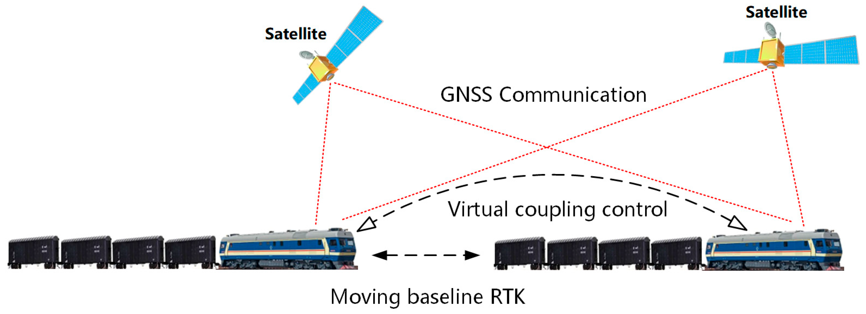
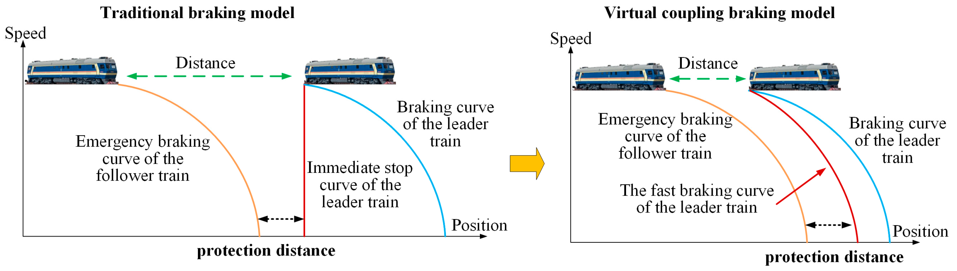
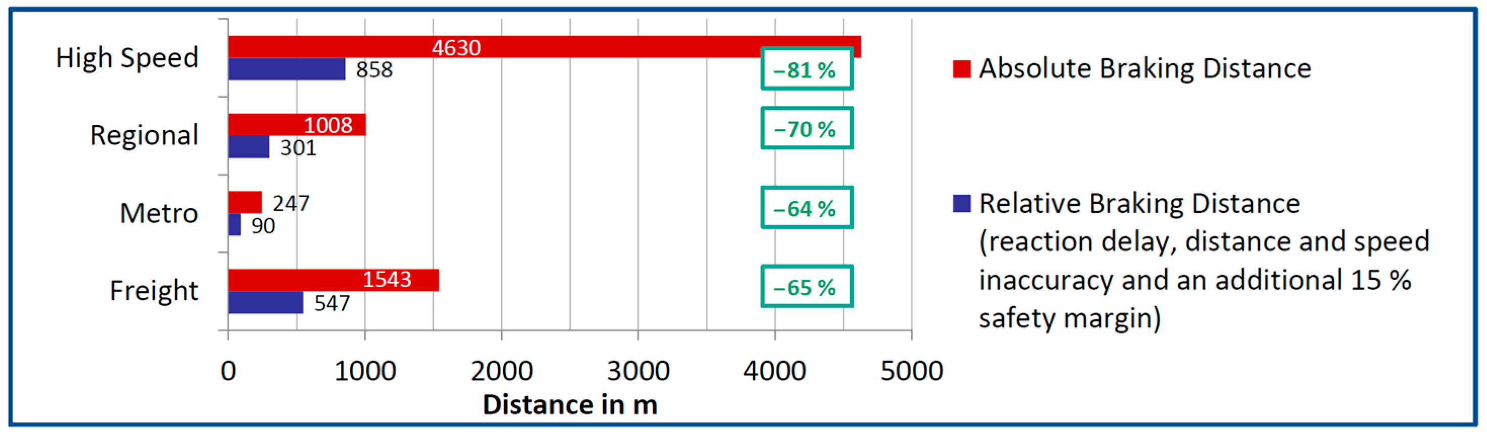
2.1. Virtual Coupling Fundamentals

Virtual coupling allows autonomous trains to operate in a dynamically coordinated manner without physical coupling, relying on precise relative positioning and synchronization between trains. Unlike traditional train operations, where safety and efficiency are ensured through physical connections or fixed signaling, VC systems require continuous real-time awareness of the relative positioning and motion states of the trains. This enables the trains to move as a cohesive unit, with close headways, while ensuring safety and operational efficiency. Achieving such coordination necessitates high-accuracy relative positioning and tight synchronization between the trains, which poses significant challenges to current train control methods.

In VC, the distance between the leading and following trains is significantly reduced compared to traditional braking models. As shown in Figure 2, the traditional braking model (absolute braking) requires a larger safety margin, as each train independently follows its braking curve. In contrast, the VC braking model (relative braking) allows the following train to dynamically adjust its braking curve to match the leader’s motion, reducing the overall protection distance.

As shown in Figure 3, there is a notable reduction in the distance between ABD and RBD. Depending on the scenario, the reduction ranges from −64% to 81%, highlighting the potential capacity improvements achieved through headway reduction when transitioning from the traditional braking model to the virtual coupling braking model. The high accuracy of relative motion tracking and the synchronization of speed, braking, and position data are therefore critical to the success of VC systems, especially in high-speed, high-density environments where small errors in synchronization can lead to operational failures.

To achieve real-time synchronization between virtually coupled trains, a dedicated vehicle-to-vehicle (V2V) wireless communication mechanism is employed. Trains exchange key data via high-speed wireless links, such as 5G-R and 400 MHz systems. This communication ensures that each train receives timely updates on the motion state of its counterpart, enabling precise spatiotemporal synchronization.

Traditional positioning systems, such as GNSS-based absolute positioning, provide limited accuracy when applied in VC settings. While effective in open areas, GNSS suffers from signal obstruction and multipath interference in tunnels and urban environments. These limitations lead to positioning errors, making it difficult to achieve the precision required for VC. Moreover, in a VC system, the relative motion of the trains needs to be tracked with high precision to ensure safe operation at short headways, which cannot be achieved with conventional GNSS-based methods that primarily focus on absolute positioning. Time synchronization between trains is also critical for coordinated movement. Even small errors in clock synchronization can cause discrepancies in speed matching, potentially destabilizing the train formation. These issues are further compounded by communication delays, which introduce latency into the system, negatively affecting synchronization. Additionally, data loss during transmission can disrupt the control system, compromising the ability to maintain safe distances and efficient operation.

To address these challenges, the MB-RTK system provides a promising solution. By utilizing differential GNSS corrections between trains, MB-RTK enhances relative positioning accuracy, reducing the impact of GNSS signal degradation and improving synchronization. This approach ensures precise inter-train motion estimation while reducing synchronization errors and delays. MB-RTK continuously refines relative positioning and motion states, ensuring safe, stable, and efficient train operation in VC systems.

2.2. Moving Baseline RTK Technology

2.2.1. Differential GNSS Processing for High Accuracy

RTK positioning enhances GNSS-based localization by leveraging differential corrections to mitigate common positioning errors and improve relative accuracy. However, traditional RTK methods rely on static base stations, which are inadequate for dynamic applications such as virtual coupling, where both the base station and rover are in continuous motion. This section presents the mathematical formulation of MB-RTK, its ambiguity resolution process, and error mitigation techniques.

In conventional RTK positioning, the raw pseudorange and carrier-phase measurements for a satellite iii at receiver $r$ can be expressed as

$$P_i^r={\rho }_i^r+c(d{t}^r-d{t}^s)+I_i^r+T_i^r+{ϵ}_i^r$$

(1)

$${\Phi }_i^r={\rho }_i^r+c(d{t}^r-d{t}^s)+I_i^r+T_i^r+\lambda N_i^r+{ϵ}_i^r$$

(2)

where $P_i^r$ and ${\Phi }_i^r$ denote the pseudorange and carrier-phase measurements, respectively. ${\rho }_i^r$ is the geometric range. $d{t}^r$ and $d{t}^s$ represent receiver and satellite clock biases. $I_i^r$ and $T_i^r$ are ionospheric and tropospheric delays. $\lambda$ is the carrier wavelength, and $N_i^r$ is the integer ambiguity. ${ϵ}_i^r$ denotes measurement noise.

To improve positioning accuracy, the double-differenced carrier-phase observation equation eliminates satellite and receiver clock biases:

$$\Delta {\mathsf{\Phi }}_{ij}^{mn}={\mathrm{u}}_{ij}^T\Delta {\mathrm{x}}^{mn}+\lambda N_{ij}^{mn}+{\epsilon }_{ij}^{mn}$$

(3)

where $\Delta {\mathrm{x}}^{mn}$ represents the relative position vector between moving reference $m$ and rover $n$. ${\mathrm{u}}_{ij}$ is the line-of-sight unit vector. $N_{ij}^{mn}$ is the integer ambiguity. ${\epsilon }_{ij}^{mn}$ represents unmodeled measurement noise.

Unlike static RTK, MB-RTK must continuously estimate the moving baseline between two trains. The state-space model for dynamic relative positioning is formulated as

$${\mathrm{x}}_{k|k-1}=F_k{\mathrm{x}}_{k-1|k-1}+G_k{\mathrm{u}}_k+{\mathrm{w}}_k$$

(4)

$${\mathrm{y}}_k=H_k{\mathrm{x}}_{k|k-1}+{\mathrm{v}}_k$$

(5)

where ${\mathrm{x}}_{k|k-1}$ represents the EKF state vector at time step $k$, including relative position, velocity, and ambiguity terms. ${\mathrm{y}}_k$ is the vector of GNSS double-differenced measurements. $F_k$, $G_k$ are the state transition matrices. $H_k$ is the observation matrix. ${\mathrm{w}}_k$, ${\mathrm{v}}_k$ denote process and measurement noise. This model allows real-time estimation of the relative position and velocity between two moving trains.

The RTK solution state transitions through different ambiguity resolution modes: NONE: No RTK solution is available due to insufficient satellite visibility or poor signal quality. L1_FLOAT: Single-frequency ambiguity remains unresolved and is treated as a floating-point estimate. NARROW_FLOAT: Dual-frequency float solution, with reduced ionospheric error but still unresolved ambiguities. L1_INT: Single-frequency integer ambiguity is resolved, improving positioning stability. NARROW_INT: The highest-precision RTK solution, where dual-frequency integer ambiguities are successfully fixed, ensuring centimeter-level accuracy.

To improve the robustness of MB-RTK, various measurement noise and outlier rejection techniques are applied. Multipath mitigation is implemented using carrier-phase smoothing to suppress multipath interference and elevation-based weighting to minimize the impact of low-elevation satellites. Adaptive measurement weighting enhances accuracy by assigning higher weights to satellites with low DOP values while reducing the influence of signals with high noise levels through SNR-based rejection. Additionally, time-consistent filtering is employed to reject GNSS measurements exhibiting abrupt phase jumps, while a moving window averaging (MWA) method is applied for redundancy checks. These strategies collectively enhance MB-RTK stability, particularly in challenging urban environments and railway applications.

To obtain centimeter-level accuracy, integer ambiguity resolution is required. The LAMBDA method is used to solve

$$\widehat{\mathrm{N}}=\arg {\min }_{N\in \mathbb{Z}}{(\tilde{N}-\mathrm{N})}^T{Q}_{\tilde{N}}^{-1}(\tilde{N}-\mathrm{N})$$

(6)

where $\widehat{\mathrm{N}}$ represents the float ambiguity estimates. $Q_{\tilde{N}}^{-1}$ is the covariance matrix of the float ambiguities.

Integer ambiguity resolution is critical to MB-RTK performance. While the LAMBDA method efficiently finds the best integer solution, additional adaptive filtering is required to prevent incorrect fixes. To enhance the robustness of MB-RTK, an adaptive ambiguity resolution strategy is applied, integrating Kalman filtering and the LAMBDA method. First, the integer ambiguity state is predicted based on prior estimates and system dynamics, using a Kalman filter to refine uncertainty and improve initial estimates. Then, the LAMBDA method is employed to resolve integer candidates by minimizing ambiguity residuals, leveraging the covariance of the float ambiguity estimates for optimal solution selection. To ensure reliability, a consistency check is performed, evaluating the variance of integer candidates. If the variance exceeds a predefined threshold, the solution is rejected, and additional observations are requested to refine ambiguity estimates. This adaptive process dynamically adjusts the ambiguity state transition model based on measurement uncertainty, effectively reducing incorrect fixes and ensuring a more stable and accurate MB-RTK solution.

Once the ambiguities are fixed, the solution transitions to the NARROW_INT mode, which provides the highest stability in MB-RTK. This allows precise relative positioning between coupled trains.

In tunnels or urban environments, GNSS signals may be temporarily lost. To ensure continuous positioning, a hybrid approach using inertial measurement units (IMU) and odometry is integrated:

$$\Delta {\mathrm{x}}^{mn}(t+\Delta t)=\Delta {\mathrm{x}}^{mn}(t)+\Delta t\cdot {\mathrm{v}}^{mn}(t)+{\displaystyle \frac{1}{2}}\Delta t^2\cdot {\mathrm{a}}^{mn}(t)$$

(7)

where ${\mathrm{v}}^{mn}$ and ${\mathrm{a}}^{mn}$ denote estimated relative velocity and acceleration.

This prediction mechanism maintains synchronization during short GNSS outages, allowing the system to recover once signals are restored.

GNSS positioning accuracy is influenced by various error sources, including satellite and receiver clock biases, ionospheric and tropospheric delays, and multipath effects. These factors introduce uncertainties in signal propagation, leading to degraded positioning precision, particularly in dynamic environments. To mitigate these issues, the dilution of precision (DOP) metric is used to assess the geometric strength of selected satellites. A lower DOP value indicates a more favorable satellite configuration, enhancing positioning accuracy and improving the reliability of RTK-based localization for VC applications. The DOP value is computed as

$$\mathrm{DOP}=\sqrt{\mathrm{trace}({({\mathrm{G}}^T\mathrm{G})}^{-1})}$$

(8)

where $\mathrm{G}$ represents the geometry matrix relating satellite positions to the receiver. A lower DOP value indicates a better satellite configuration, leading to improved positioning accuracy. This factor plays a critical role in the practical deployment of RTK-based localization for VC applications.

The accuracy of MB-RTK solutions depends not only on integer ambiguity resolution but also on the cumulative effect of error sources such as satellite geometry, atmospheric interference, and dynamic motion errors. The general error propagation model in the MB-RTK system can be expressed as

$$\delta {\mathrm{x}}_{relative}={\mathrm{G}}^{-1}(\delta \mathrm{P}+\delta \mathrm{I}+\delta \mathrm{T}+\delta \mathrm{N}+\delta \mathrm{M})$$

(9)

where $\delta {\mathrm{x}}_{relative}$ represents the propagated relative positioning error. $\delta \mathrm{P}$ is the pseudorange error. $\delta \mathrm{I}$, $\delta \mathrm{T}$ are the ionospheric and tropospheric error components. $\delta \mathrm{N}$ is the ambiguity error, which significantly impacts the precision before ambiguity resolution. $\delta \mathrm{M}$ represents multipath interference effects. ${\mathrm{G}}^{-1}$ is the geometry dilution matrix, which translates measurement errors into positioning uncertainty.

This equation highlights that MB-RTK error propagation is directly influenced by satellite geometry (DOP) and error mitigation strategies. A poor satellite configuration (high DOP value) amplifies the impact of atmospheric and ambiguity errors.

Simultaneously solving for ${\mathrm{r}}_{\mathrm{relative}}$ and $\Delta \Delta N_{ij}$ is a critical step in the MB-RTK system, typically achieved through a least-squares optimization framework:

$${\min }_{r_{\mathrm{relative}},\Delta \Delta N_{ij}}{\displaystyle \sum _{ij}{\left(\nabla \Delta {\varphi }_{ij}-({\mathrm{u}}_{ij}^T{\mathrm{r}}_{\mathrm{relative}}+\lambda \Delta \Delta N_{ij})\right)}^2}$$

(10)

This optimization minimizes residuals by integrating satellite geometry and measurement noise covariance, thereby ensuring centimeter-level precision in the computed relative position.

By employing these advanced error mitigation strategies, MB-RTK enhances relative positioning accuracy, ensuring stable and precise localization for virtual coupling applications. The next section further explores how MB-RTK integrates these techniques into a real-time synchronization framework, enabling robust inter-train coordination in high-speed railway networks.

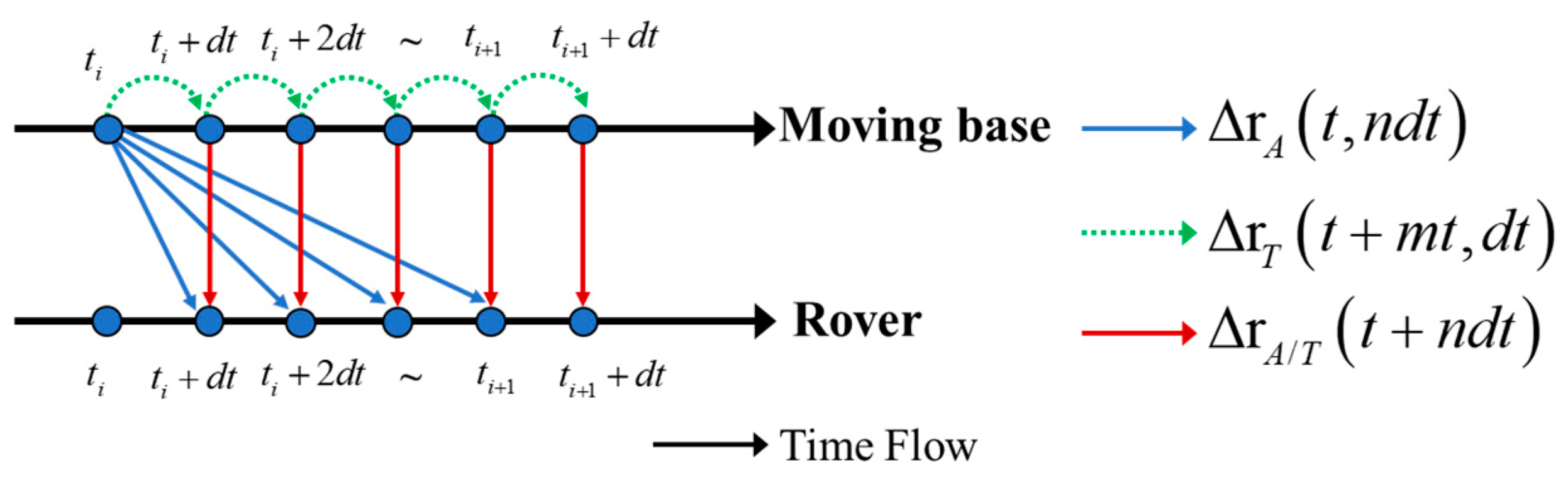
2.2.2. Dynamic Baseline Estimation

The MB-RTK system is a high-precision relative positioning technology based on GNSS, designed to estimate real-time relative position and velocity between dynamic platforms. Unlike conventional RTK, which relies on fixed reference stations for absolute positioning, MB-RTK establishes a dynamic reference by leveraging inter-platform carrier-phase differencing. This enables high-precision relative positioning even in scenarios where GNSS signal degradation, multipath interference, and baseline variations present significant challenges.

Compared to traditional RTK, MB-RTK offers several advantages, particularly in the context of VC. Standard RTK techniques, which require a stationary base station, struggle in high-speed railway applications due to limitations in baseline length, frequent reference station handovers, and dependency on fixed infrastructure. In contrast, MB-RTK dynamically computes the relative position between moving trains, maintaining high accuracy without reliance on external ground stations. This adaptability makes it a more suitable approach for real-time, high-precision train coordination in VC operations.

To further enhance the robustness of MB-RTK in dynamic train operations, an adaptive ambiguity resolution mechanism is integrated. This mechanism continuously monitors GNSS signal quality and adjusts the ambiguity resolution process accordingly. When signal conditions are stable, the system attempts to fix integer ambiguities (NARROW_INT) to achieve centimeter-level precision. However, in environments where GNSS signals experience degradation—such as tunnels or urban canyons—the system temporarily switches to a float solution (NARROW_FLOAT) while accumulating more observations to improve resolution reliability. This hybrid approach minimizes incorrect ambiguity fixes, thereby enhancing overall system stability.

Dynamic baseline estimation further enhances traditional GNSS-based positioning by incorporating real-time train motion dynamics. In conventional RTK, relative positioning updates are constrained by static baseline assumptions, making them less effective for rapidly changing environments. By leveraging train motion models, MB-RTK continuously refines relative positioning estimates, reducing the impact of transient GNSS errors and providing greater localization stability. Additionally, a dynamic DOP (dilution of precision) optimization strategy is implemented to improve positioning accuracy in VC applications. By dynamically selecting and weighting satellites based on their contribution to DOP reduction, the system minimizes the geometric dilution effect, ensuring consistent precision in relative positioning.

In dynamic baseline scenarios, the relative position is computed as

$$r_{\mathrm{relative}}\left(t_r\right)=r_r\left(t_r\right)-r_b\left(t_b\right)$$

(11)

where $r_r\left(t_r\right)$ and $r_b\left(t_b\right)$ represent the positions of the leading and following trains (or rover and base station) at times $t_r$ and $t_b$, respectively. The relative velocity is further derived as

$$v_{relative}={\displaystyle \frac{d{\mathrm{r}}_{\mathrm{relative}}\left(t_r\right)}{dt}}$$

(12)

MB-RTK employs an extended Kalman filter (EKF) to estimate the state vector, enabling precise prediction and updating of the relative position and velocity. By integrating GNSS observation data, the EKF effectively refines state estimates, ensuring robustness against noise and ambiguity. This is particularly critical in dynamic railway environments where factors such as acceleration changes, track curvature variations, and inter-train communication delays can introduce additional localization uncertainties.

Figure 4 illustrates the process of calculating the relative position between the moving base station and the rover by analyzing variations in observational data over time. The blue solid arrows represent direct observations between the moving base station and the rover, while the green dashed arrows indicate dynamically evolving changes in the rover’s motion. The red solid arrows depict the accumulated variations in relative position over time. This process effectively demonstrates the core principle of the MB-RTK framework: accurately estimating the movement trajectory and relative position to the base station over continuous observation periods.

Besides this, Figure 4 also demonstrates the importance of real-time ambiguity resolution and adaptive satellite selection strategies. As MB-RTK continuously estimates the train-to-train baseline, the system dynamically adjusts integer ambiguity resolution (FLOAT to INT transitions) based on signal quality. The solid red arrows in Figure 4 highlight how ambiguity resolution status may change due to GNSS fluctuations, while the green arrows represent adaptive DOP-based satellite selection improving positioning accuracy. This enables robust virtual coupling, even under varying GNSS conditions.

One of the key benefits of MB-RTK in virtual coupling applications is its ability to maintain precise synchronization between coupled trains. Unlike conventional systems that rely solely on train-to-train communication for relative positioning, MB-RTK provides real-time inter-train localization updates, reducing reliance on external data exchange. This is particularly beneficial in scenarios where communication bandwidth is limited or intermittent, such as tunnels or areas with electromagnetic interference.

To further enhance the robustness of dynamic baseline estimation under GNSS signal interruptions, a machine-learning-driven approach is proposed as an extension of this research. By leveraging historical data and predictive modeling, the system can estimate relative position and velocity when GNSS data are temporarily unavailable:

$$r_{\mathrm{relative}}(t)=f_{\mathrm{ML}}(r_{\mathrm{relative}}(t-n:t-1),v_{\mathrm{relative}}(t-n:t-1))$$

(13)

where $f_{\mathrm{ML}}$ represents a neural-network-based predictive model trained on historical baseline data, and $n\cdot t$ denotes the length of the historical observation window. This predictive method serves as a supplementary approach to mitigate localization degradation in the absence of GNSS updates. While this study primarily focuses on MB-RTK estimation, such predictive enhancements offer promising avenues for future research in real-time railway localization under challenging GNSS conditions.

2.3. Spatiotemporal Synchronization Requirements

Achieving robust spatiotemporal synchronization is critical for VC, where multiple trains must continuously coordinate their positions, velocities, accelerations, and timing references in real time. Any discrepancies in synchronization can lead to safety risks and degraded operational efficiency. To ensure smooth and stable VC operations, synchronization must be maintained across all relevant motion parameters within strict tolerances.

In a multi-train system, let the $i$-th train’s state at time $t$ be represented by a vector

$$S_i(t)={[x_i(t), v_i(t), a_i(t), t_i]}^T$$

(14)

where $x_i(t)$ is the train’s position, $v_i(t)$ its velocity, $a_i(t)$ its acceleration, and $t_i$ denotes the train’s local time reference. Effective spatiotemporal synchronization requires that these states remain consistent across all trains within a specified tolerance. Commonly, the following metrics are used to quantify spatiotemporal performance:

Maintaining precise relative positioning is essential to ensure safe inter-train spacing. Excessive deviations in train positions can cause undesired fluctuations in headways, leading to unstable train formations. The maximum allowable difference between the positions of two adjacent trains at a given reference time is given by

$$\Delta x_{ij}(t) = \left|x_i(t) - x_j(t)\right| \le {ϵ}_x$$

(15)

where ${ϵ}_x$ is the position tolerance threshold defined by safety regulations.

Velocity synchronization is equally crucial for maintaining stable formation. Even small mismatches in train speeds can accumulate over time, causing relative drift between trains and necessitating frequent speed adjustments. This effect is quantified as

$$\Delta v_{ij}(t) = \left|v_i(t) - v_j(t)\right| \le {ϵ}_v$$

(16)

where ${ϵ}_v$ defines the maximum allowable velocity difference to ensure smooth coordination and energy efficiency.

Beyond position and velocity alignment, ensuring consistent acceleration is necessary to prevent abrupt changes in train dynamics. Sudden variations in acceleration introduce unwanted jerk, which can negatively impact both ride comfort and train stability. To minimize these effects, the acceleration difference between trains is constrained by

$$\Delta a_{ij}(t) = \left|a_i(t) - a_j(t)\right| \le {ϵ}_a$$

(17)

where ${ϵ}_a$ bounds acceleration discrepancies, reducing abrupt force variations and promoting smooth transitions in train operations.

Time synchronization also plays a crucial role in VC systems. Since each train operates on an independent local clock, even minor offsets in time references can cause discrepancies in shared state updates, leading to misalignment in motion coordination. To ensure accurate data fusion, the local time difference between any two trains must satisfy

$$\Delta t_{ij} = \left|t_i-t_j\right| \le {ϵ}_t$$

(18)

where ${ϵ}_t$ represents the maximum permissible clock offset to maintain spatiotemporal consistency.

The MB-RTK framework offers a promising solution to these synchronization challenges. By leveraging inter-train differential GNSS corrections, MB-RTK significantly enhances relative positioning accuracy, reducing spatial errors and improving velocity alignment. Furthermore, MB-RTK inherently facilitates time synchronization by utilizing GNSS-based timestamps, mitigating clock drift between moving platforms. These advantages make MB-RTK particularly well-suited for virtual coupling applications, where precise real-time coordination is a fundamental requirement.

Taken together, these considerations highlight the necessity of integrating high-precision relative positioning, low-latency communication, and robust predictive control to achieve reliable spatiotemporal synchronization in train virtual coupling systems. Only through consistent alignment of motion parameters and timing references can virtual coupling fully unlock its potential, improving both capacity and operational flexibility in future railway networks.

3. System Implementation

3.1. Dynamic Model of Virtual Coupling

VC relies on a precise dynamic model to ensure smooth inter-train coordination. This section introduces a motion modeling framework that considers traction, braking, aerodynamic drag, and curvature resistance, establishing the foundation for real-time synchronization and control.

The dynamics of virtually coupled trains are governed by Newtonian motion, where each train in the formation is subject to multiple forces influencing its acceleration, deceleration, and response to environmental disturbances such as wind resistance and terrain variations. Each train is modeled as a mass point subjected to external forces, leading to the following motion equation:

$$m_i{\displaystyle \frac{d{v}_i}{dt}}=F_{\mathrm{tr},i}-F_{\mathrm{br},i}-F_{\mathrm{air},i}-F_{\mathrm{curve},i}$$

(19)

where $m_i$ is the mass of train $i$, and the right-hand side terms denote traction force $F_{\mathrm{tr},i}$, braking force $F_{\mathrm{br},i}$, aerodynamic drag $F_{\mathrm{air},i}$, and curvature resistance $F_{\mathrm{curve},i}$, respectively.

The traction force is generated by the propulsion system and depends on the available power and efficiency of the train’s drive system:

$$F_{\mathrm{tr},i}=\eta {\displaystyle \frac{P_i}{v_i}}$$

(20)

where $P$ is the traction power, and $\eta$ is the mechanical efficiency.

The braking force follows a deceleration function based on braking torque and adhesion conditions, given by

$$F_{\mathrm{br},i}=C_b{m}_{i}g$$

(21)

where $C_b$ represents the braking coefficient, and $g$ is gravitational acceleration.

Air resistance, which plays a significant role at higher speeds, is described using the quadratic drag model:

$$F_{\mathrm{air},i}={\displaystyle \frac{1}{2}}{C}_d\rho A{v}_i^2$$

(22)

where $C_d$ is the drag coefficient, $\rho$ is air density, and $A$ is the frontal cross-sectional area of the train.

When traversing curved sections, trains also experience additional resistance, modeled as

$$F_{\mathrm{curve},i}={\displaystyle \frac{m_i{v}_i^2}{R}}$$

(23)

where $R$ is the track curvature radius. This term increases as the curve tightens, requiring adaptive speed regulation.

Unlike conventional train control, virtual coupling relies on dynamic inter-train synchronization rather than fixed physical spacing. The relative motion between coupled trains is regulated through velocity matching and spacing regulation, ensuring smooth and stable operation. The general motion equation for inter-train synchronization can be expressed as

$${\displaystyle \frac{d{v}_{i+1}}{dt}}={\displaystyle \frac{1}{m_{i+1}}}(F_{tr,i+1}-F_{br,i+1}-F_{air,i+1}-F_{curve,i+1})+u_{sync,i}$$

(24)

where $u_{sync,i}$ represents a synchronization control input, which adjusts the following train’s speed based on the relative position and velocity of the leading train.

A proportional-differential synchronization law is introduced to enforce spatiotemporal consistency:

$$u_{sync,i}=K_p(\Delta x_i-d_{safe})+K_v(\Delta v_i)$$

(25)

where $K_p$ is the position control gain, ensuring inter-train spacing remains within a predefined safety margin $d_{safe}$. $K_v$ is the velocity correction gain, reducing speed mismatches and preventing abrupt acceleration/deceleration differences.

This model effectively captures the essential characteristics of virtual coupling, ensuring high-precision inter-train coordination while accounting for real-world operational constraints. The subsequent sections explore the integration of MB-RTK technology to enhance synchronization accuracy and robustness.

This motion model effectively captures the essential characteristics of VC, ensuring high-precision inter-train coordination while accounting for real-world operational constraints. In addition to motion modeling, precise localization is crucial for VC, as train positioning errors can propagate through the formation, leading to synchronization degradation.

3.2. Spatiotemporal Synchronization and Communication

3.2.1. Spatiotemporal Synchronization Mechanism

The MB-RTK framework plays a central role in synchronization by providing accurate relative positioning $\Delta x_{ij}(t)$ and velocity $\Delta v_{ij}(t)$ measurements between trains. Synchronization ensures that inter-train spacing, speed, and timing remain consistent, minimizing deviations that could impact VC stability and operational efficiency.

To maintain a stable inter-train formation, the spacing between adjacent trains should remain close to a predefined reference distance $d_{safe}$. Any deviation from this reference distance is corrected using a proportional control law:

$$x_j^{\mathrm{corr}}(t)=x_j(t)+K_p(\Delta x_{ij}(t) -d_{safe})$$

(26)

where $K_p$ is the proportional gain that controls the adjustment. This correction minimizes deviations from the desired spacing, ensuring smooth operation in close-proximity VC scenarios.

Beyond spatial alignment, velocity synchronization is crucial for maintaining stable relative motion. Any discrepancy in relative velocity is corrected dynamically, ensuring that the trailing train maintains a consistent speed within the convoy:

$$v_j^{\mathrm{corr}}(t)=v_j(t)-K_v\Delta v_{ij}(t)$$

(27)

where $K_v$ is the velocity correction gain. By adjusting velocity in response to real-time measurements, the system ensures smooth motion coordination, reducing energy inefficiencies and avoiding sudden accelerations or decelerations.

Accurate time synchronization is essential for maintaining consistency in data exchange and synchronization commands across multiple trains. MB-RTK identifies clock offsets $\Delta t_{ij}$ and applies a correction mechanism:

$$t_j^{\mathrm{corr}}=t_j-K_t\Delta t_{ij}$$

(28)

where $K_t$ is the time correction gain. This adjustment aligns timestamps across all trains, ensuring that data processing and control decisions remain consistent within the VC framework.

To enhance synchronization performance, an adaptive gain adjustment algorithm is introduced. This algorithm dynamically tunes $K_p$, $K_v$, and $K_t$ based on residual errors $Res\left(t\right)$, communication delays, and environmental noise. The gain update rule is defined as

$$K_p(t+1)=K_p(t)+\alpha \cdot Res(t)$$

(29)

where $\alpha$ represents the learning rate. This adaptive mechanism ensures that synchronization responses remain stable under varying operational conditions. By dynamically adjusting gains, the system improves responsiveness while avoiding excessive corrections that could introduce oscillations or instability.

The synchronization problem can be formulated as a multi-objective optimization problem to minimize deviations in position, velocity, and time while incorporating practical system constraints. The cost function is expressed as

$${\mathrm{m}\mathrm{i}\mathrm{n}}_{p_j,v_j,t_j} J={\int }_0^T\left[K_p{\left(\Delta x_{ij}\left(t\right)-s_{\mathrm{R}\mathrm{D}\mathrm{B}\mathrm{M}}\right)}^2+K_v{\left(\Delta v_{ij}\left(t\right)\right)}^2+K_t{\left(\Delta t_{ij}\right)}^2\right]dt$$

(30)

To ensure practical implementation, additional constraints must be considered, such as physical acceleration limits, control update frequency, and communication latency. These constraints prevent excessive corrections and ensure stable synchronization in real-world VC operations.

3.2.2. Decentralized Synchronization Algorithm

Efficient communication mechanisms are essential for transmitting MB-RTK outputs and achieving spatiotemporal synchronization in VC systems. Traditional centralized synchronization architectures rely on a single control node to compute and distribute synchronization corrections for all trains. While effective for small-scale implementations, this approach imposes significant bandwidth demands and suffers from single-point failures. Additionally, as the number of coupled trains increases, the communication and computation load grow quadratically with the network size, limiting scalability.

To address these limitations, we propose a decentralized distributed synchronization algorithm, which allows each train to compute its own synchronization corrections based on local measurements and minimal shared information with nearby neighbors. This framework significantly reduces communication overhead and enhances system scalability.

In the proposed distributed scheme, each train exchanges synchronization information only with its immediate neighbors, forming a localized communication topology rather than transmitting all state information to a centralized controller. This approach mitigates bandwidth congestion and avoids the latency-sensitive bottlenecks of centralized architectures. The required local communication frequency $f_{\mathrm{comm}}$ depends on the network size and communication constraints, modeled as

$$f_{\mathrm{comm}}={\displaystyle \frac{1}{T_{\mathrm{consensus}}}}\propto {\displaystyle \frac{\log N}{{\tau }_{\max }}}$$

(31)

where $N$ is the number of trains in the network. The logarithmic scaling ensures that communication overhead grows only marginally as the system expands, making it well-suited for high-density railway networks.

However, communication delays introduce latency in state updates, which can degrade synchronization performance. If the delay τ exceeds a critical threshold, the consensus process may struggle to converge, leading to oscillations or desynchronization. To mitigate this, an adaptive delay compensation mechanism can be incorporated into the consensus model to ensure stable and accurate synchronization.

To achieve synchronization, the algorithm employs a dynamic consensus model, allowing each train to iteratively adjust its position and velocity based on the relative state differences with its neighbors. The synchronization dynamics for position and velocity are formulated as

$${\dot{x}}_j(t)={\displaystyle \sum _{k\in {\mathcal{N}}_j}{a}_{jk}}(t)(x_k(t-{\tau }_c)-x_j(t))$$

(32)

$${\dot{v}}_j(t)={\displaystyle \sum _{k\in {\mathcal{N}}_j}{b}_{jk}}(t)(v_k(t-{\tau }_c)-v_j(t))$$

(33)

where $a_{jk}\left(t\right)$ and $b_{jk}\left(t\right)$ are time-varying consensus weights satisfying ${\displaystyle \sum _k{a}_{jk}}=1$, and ${\tau }_c$ represents the communication delay. By relying on localized updates rather than system-wide computations, this consensus-based approach ensures that all trains gradually converge to a synchronized state without requiring global coordination.

To further mitigate the impact of communication delays and packet loss, each train applies an extended Kalman filter (EKF) for real-time state prediction and correction. The state prediction model is given by

$${\widehat{\mathrm{S}}}_j(t+1|t)=F_j{\mathrm{S}}_j(t)+G_j{\mathrm{U}}_j(t)+{\mathrm{w}}_j(t)$$

(34)

$$P_j(t+1|t)=F_j{P}_j(t)F_j^T+Q_j$$

(35)

where $F$ is the state transition matrix, $G_j$ accounts for control inputs, and ${\mathrm{w}}_j(t)~\mathcal{N}(0,Q_j)$ represents process noise. Observational updates refine predictions based on GNSS and IMU measurements:

$$K_j(t)=P_j(t|t-1)H_j^T{(H_j{P}_j(t|t-1)H_j^T+R_j)}^{-1}$$

(36)

$${\widehat{\mathrm{S}}}_j(t|t)={\widehat{\mathrm{S}}}_j(t|t-1)+K_j(t)(z_j(t)-H_j{\widehat{\mathrm{S}}}_j(t|t-1))$$

(37)

$$P_j(t|t)=(I-K_j(t)H_j)P_j(t|t-1)$$

(38)

where $K_j(t)$ is the Kalman gain, and $H_j$ maps the state vector to sensor measurements. By dynamically refining state estimates, this framework ensures robust local synchronization even under intermittent communication failures.

To further enhance synchronization reliability, we integrated forward error correction (FEC) and predictive retransmission mechanisms. A Reed–Solomon error correction scheme is employed:

$$C_j(t)=\mathcal{E}({\mathrm{S}}_j(t))=[s_1,s_2,\dots ,s_n]\cdot G_{RS}$$

(39)

where $G_{RS}$ is the generator matrix. If the synchronization error exceeds a predefined threshold ${ϵ}_{\mathrm{sync}}$, retransmissions are triggered:

$$\Vert {\widehat{\mathrm{S}}}_j(t)-{\widehat{\mathrm{S}}}_k(t)\Vert >{ϵ}_{\mathrm{sync}}\Rightarrow {\mathrm{Request} \mathrm{retransmission} \mathrm{of} \mathrm{S}}_k(t-\Delta t)$$

(40)

This predictive retransmission mechanism ensures that synchronization remains accurate even in the presence of communication disruptions.

To better illustrate the advantages of the proposed decentralized synchronization framework,

Table 1. Comparison between centralized and distributed synchronization in VC systems.

Aspect	Centralized Synchronization	Distributed Synchronization
Communication load	High: All state vectors $S_j\left(t\right)$ sent to a central node, requiring high bandwidth.	Low: Only relative states (position, velocity) with neighbors are exchanged. Communication reduced by ~60%.
Latency sensitivity	High: Single-point failure or delay ${\tau }_c>{\tau }_{max}$ affects the entire system.	Low: Local calculations reduce reliance on network latency. Tolerates delays up to $3{\tau }_{max}$ with minimal errors.
Scalability	Limited: Bandwidth and computation grow quadratically with the number of trains $N$.	High: Communication scales linearly with local neighborhood size. Consensus algorithm complexity is $O\left(logN\right)$.
Robustness	Vulnerable: Central node failure can disrupt the entire system.	Resilient: Localized corrections and fault-tolerant consensus ensure operation during interruptions.
Implementation complexity	Moderate: Requires a centralized controller with high computational power.	Moderate-High: Requires onboard processing but eliminates the need for a central node.
Error tolerance	Low: Sensitive to synchronization errors under high latency or packet loss.	High: Distributed error correction and predictive algorithms ensure accurate state estimation.

compares centralized and distributed synchronization approaches in virtual coupling systems. The comparison is derived from a comprehensive analysis conducted by the authors, based on relevant literature and practical considerations [1].

The integration of MB-RTK outputs with robust distributed synchronization strategies forms the backbone of spatiotemporal synchronization in VC systems. This approach ensures high-accuracy alignment of position, velocity, and time across coupled trains while reducing bandwidth demands and computational overhead. By addressing challenges such as communication delays and environmental disturbances, the proposed synchronization framework provides a scalable and resilient solution for future railway networks, supporting high-density and autonomous train operations.

4. Experimental Results

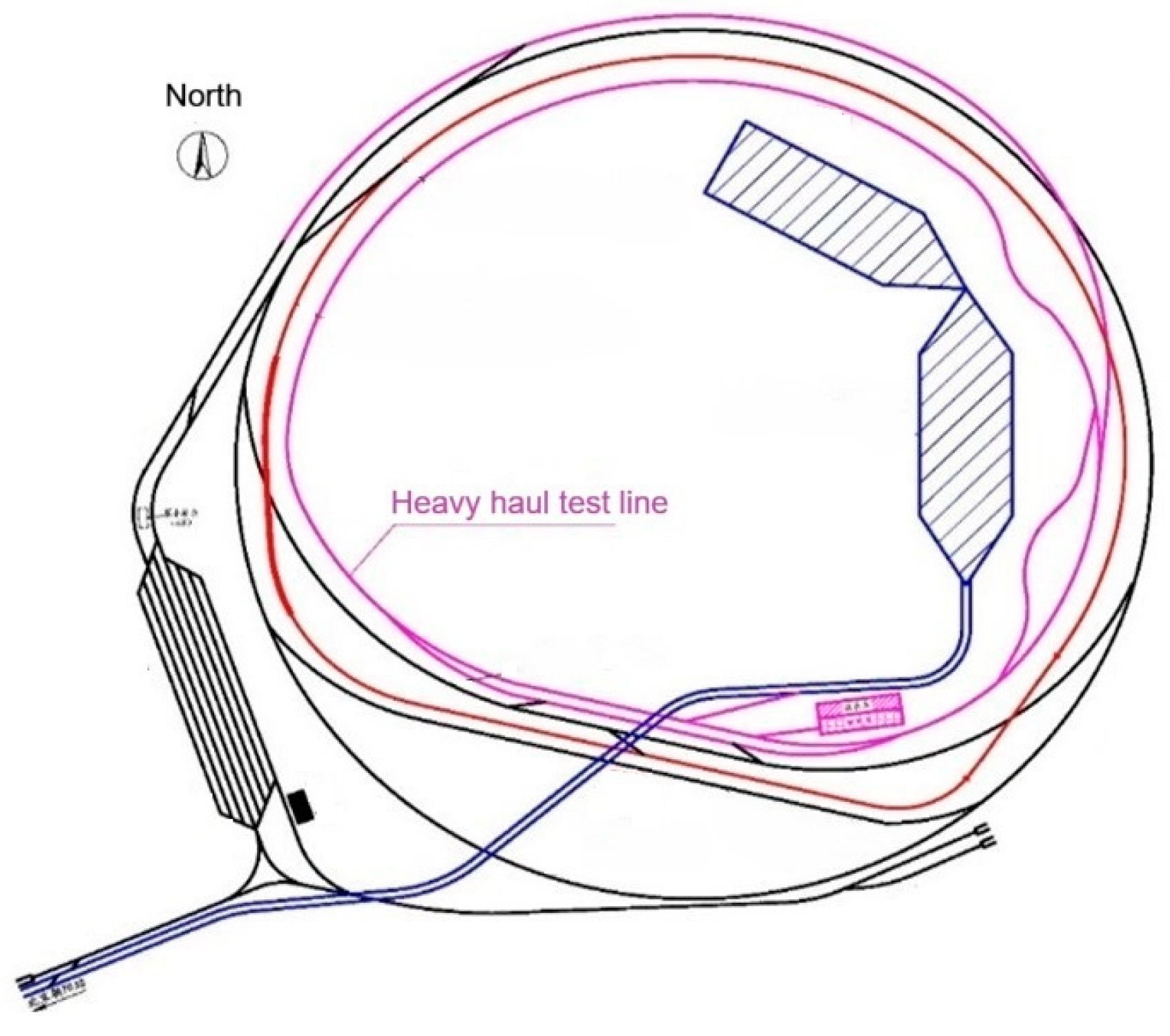
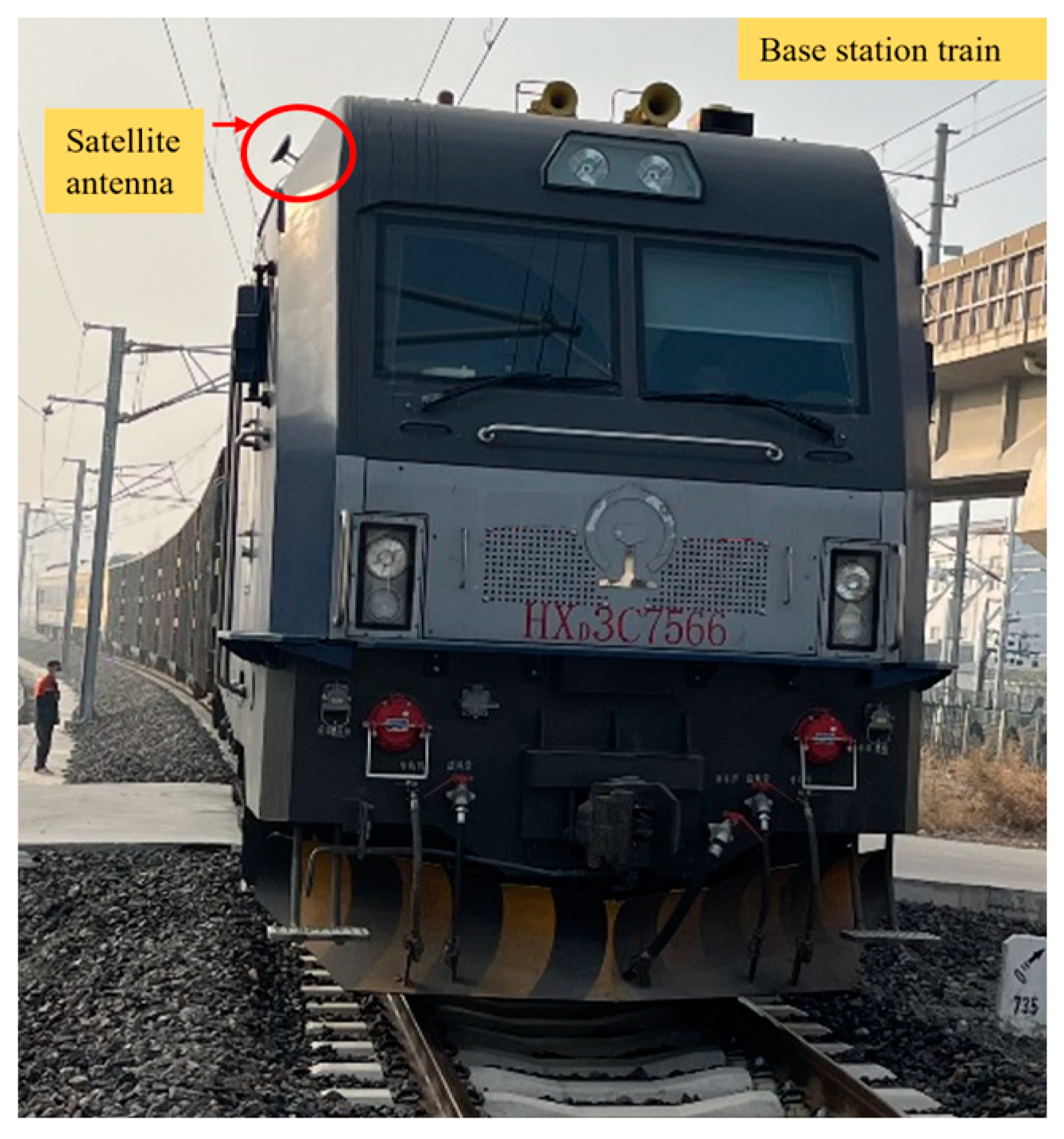
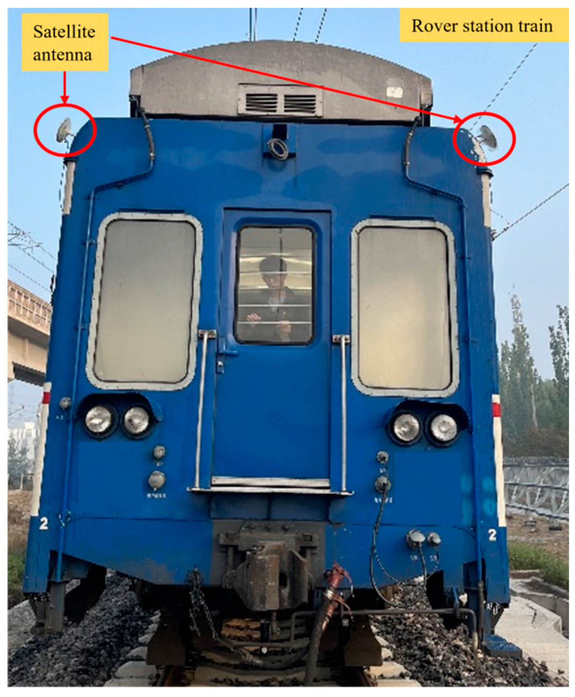
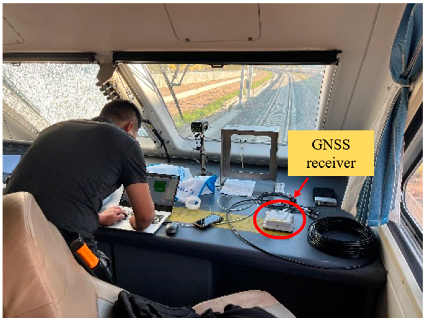
4.1. Experimental Environment and Setup

The application of the GNSS-based moving baseline RTK method in train virtual coupling systems requires thorough validation to ensure both reliability and accuracy. This chapter presents field tests conducted to evaluate the system’s performance across various operating scenarios and provides a comprehensive analysis of the test data. The primary objective of these experiments is to assess the MB-RTK framework’s accuracy in relative positioning, evaluate its impact on train synchronization, and validate its robustness under real-world railway conditions.

The experiments were conducted on a near-elliptical closed-loop railway track, designed to replicate real-world operating conditions. As shown in Figure 5, the leading train (base station) was an HXD3C electric locomotive, while the following train (rover station) was a comprehensive inspection train, as illustrated in Figure 6, Figure 7 and Figure 8. The system incorporated GNSS receivers and real-time communication modules to enable synchronized control and data exchange. The experimental design considered installation constraints and test diversity, with the GNSS antenna mounted at an inclination for optimal satellite visibility, the leading train using a single antenna for reference positioning, and the following train employing dual antennas to enhance positioning stability and attitude determination.

To comprehensively evaluate the MB-RTK system, both absolute and relative positioning data were collected. Absolute metrics included latitude, longitude, height, and velocity components in north, east, and up directions. These measurements were used to assess individual train localization accuracy. Relative metrics, including inter-train distance, relative speed, and RTK fix status, were used to evaluate the performance of virtual coupling. Key evaluation metrics focused on positioning accuracy, velocity estimation, RTK fix stability, and synchronization performance. Absolute position error was analyzed by comparing GNSS-based positioning with reference ground truth. Relative position error measured the deviation in inter-train distance estimates under MB-RTK corrections. Velocity error was quantified as the difference between the measured and expected velocity. The RTK fix ratio indicated the percentage of time MB-RTK maintained a fixed solution, ensuring high-precision relative positioning. Additionally, time offset was used to assess synchronization latency between coupled trains.

These collected data and computed metrics provide the foundation for evaluating the MB-RTK framework’s performance. The following sections will analyze tracking performance, RTK stability, and spatiotemporal synchronization metrics to validate the effectiveness of the proposed approach.

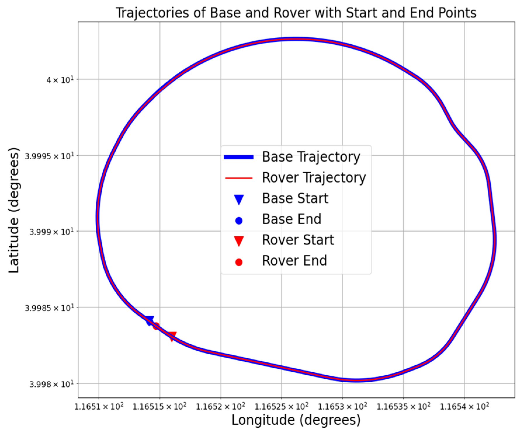
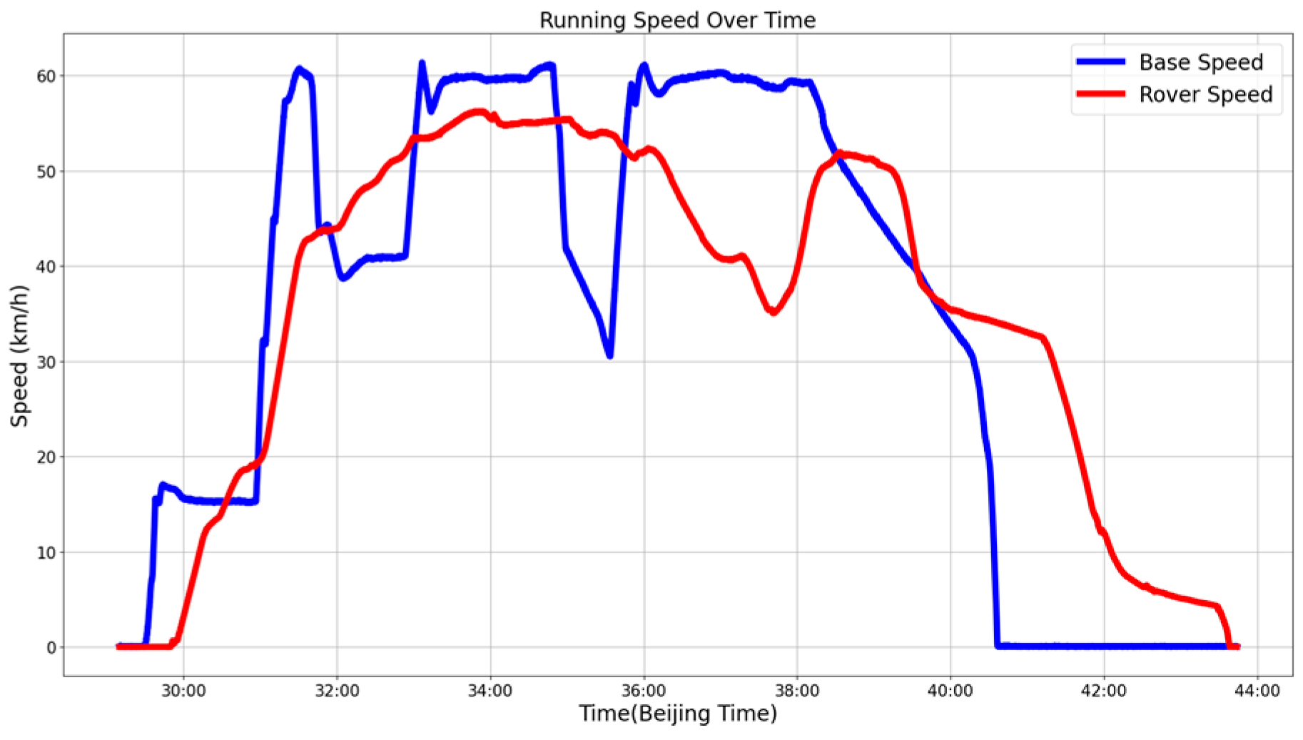
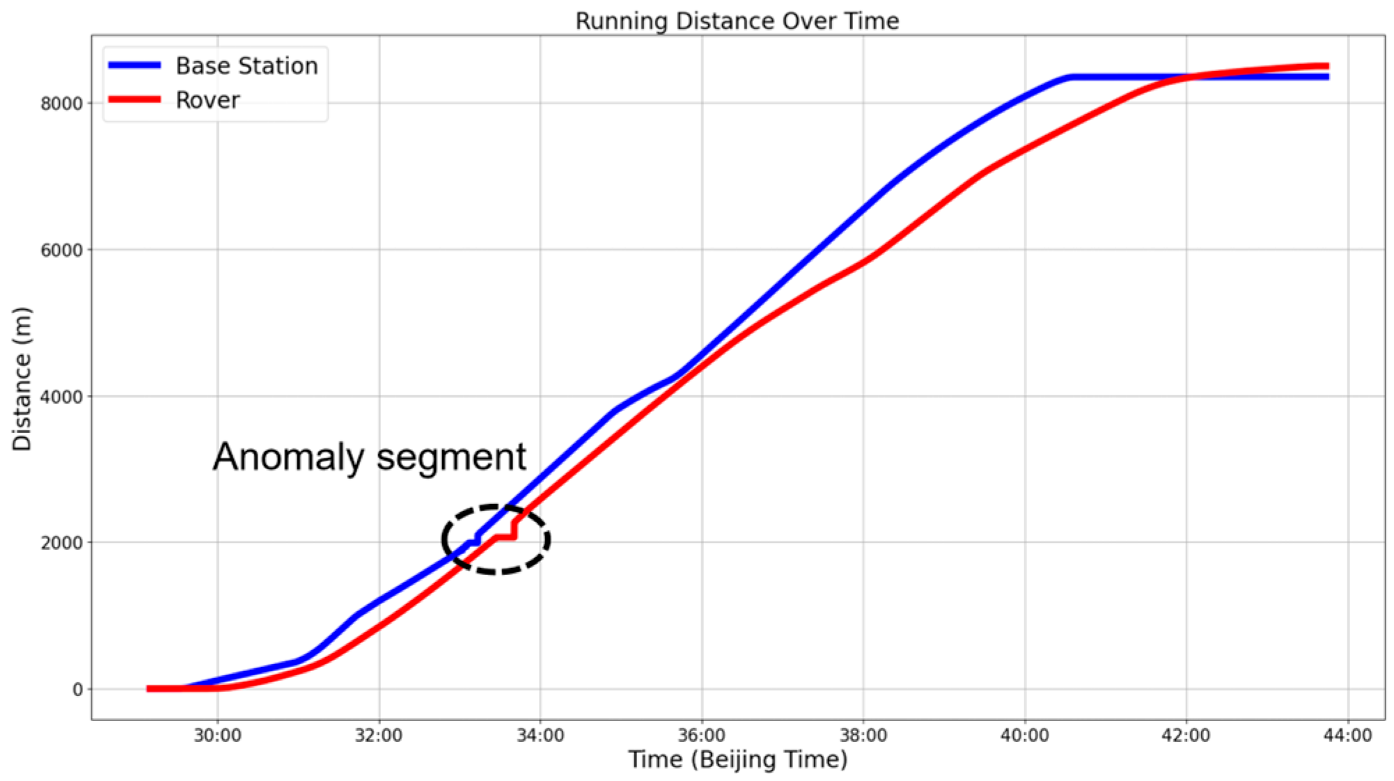
4.2. Overall Tracking Performance

Figure 9 illustrates the trajectories of the leading train (Base Station, blue curve) and the following train (Rover Station, red curve) on a closed-loop track. Initially separated by 200 m, the leading train returns to its starting point after completing one lap, while the following train stops closer to the leading train. These results demonstrate the system’s capability to maintain relative positioning, validating the trajectory tracking performance of the virtual coupling system in a closed-loop environment.

Figure 10 depicts the speed profiles during the tracking process, The horizontal axis is the simplified Beijing time, and the vertical axis is the speed (km/h). The leading train initiates deceleration at 34:49, while the following train exhibits a noticeable delay, starting deceleration at 35:00 with a significantly lower braking rate. By 35:34, a critical speed disparity emerges: the leading train’s speed drops to 30 km/h, whereas the following train maintains 55 km/h, indicating a synchronization delay. This discrepancy highlights potential collision risks and suggests suboptimal synchronization performance during dynamic deceleration scenarios.

Figure 11 further analyzes inter-train proximity between 34:49 and 36:00, showing irregularities in the distance curve within the dashed region. These deviations may result from GNSS signal occlusion or environmental interference, causing temporary inconsistencies in position tracking. Further investigation is required to identify the root cause and enhance system robustness.

Overall, the experimental results confirm that the MB-RTK framework provides accurate and reliable trajectory tracking. The system effectively synchronizes position, velocity, and inter-train distance, achieving the level of coordination required for virtual coupling. However, challenges remain in maintaining synchronized speed profiles, particularly during dynamic braking phases. The observed irregularities in the distance curve suggest a need for improved anti-interference mechanisms. Enhancing real-time speed synchronization remains a critical challenge, requiring further research to improve system reliability and safety.

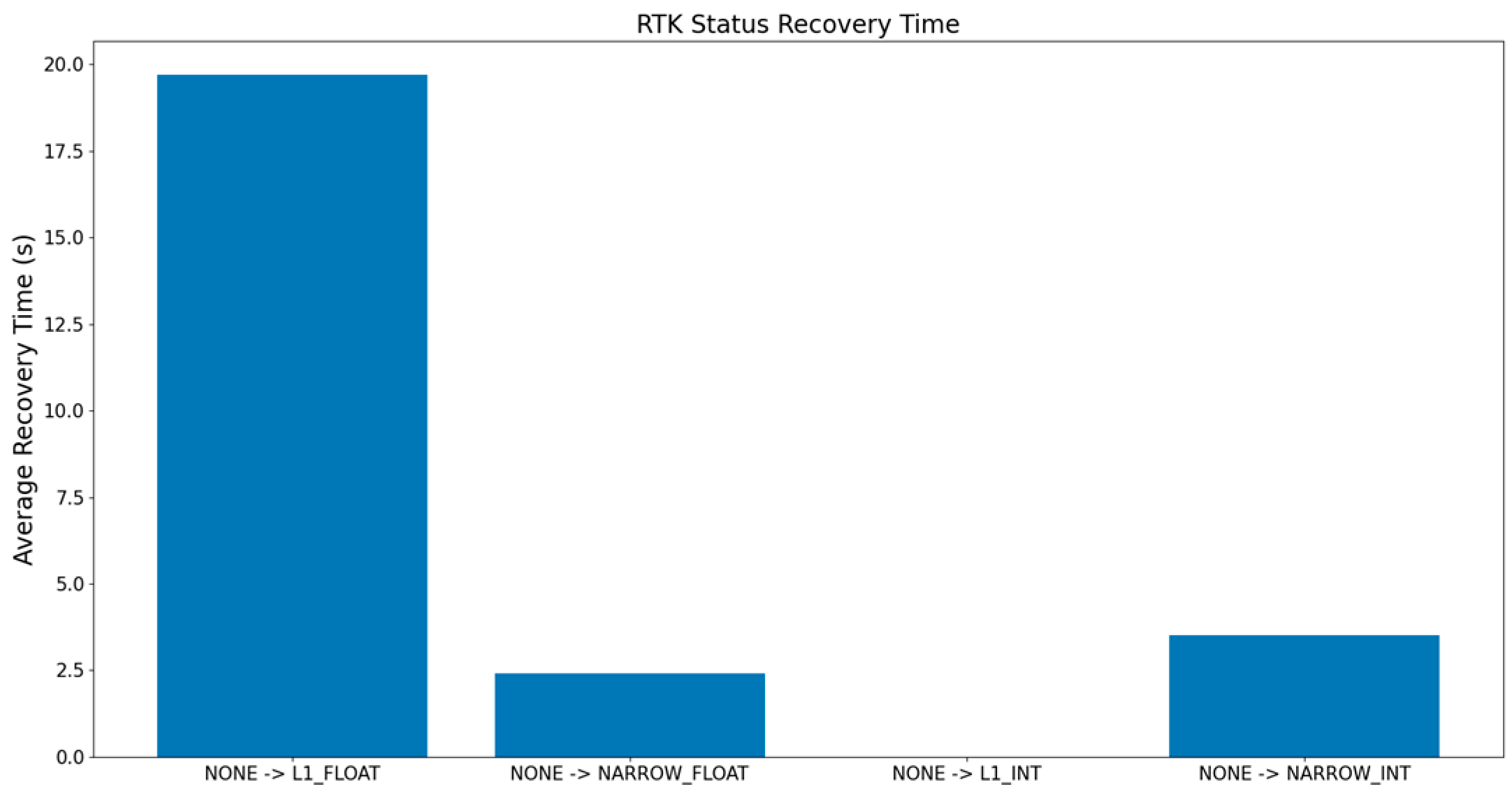
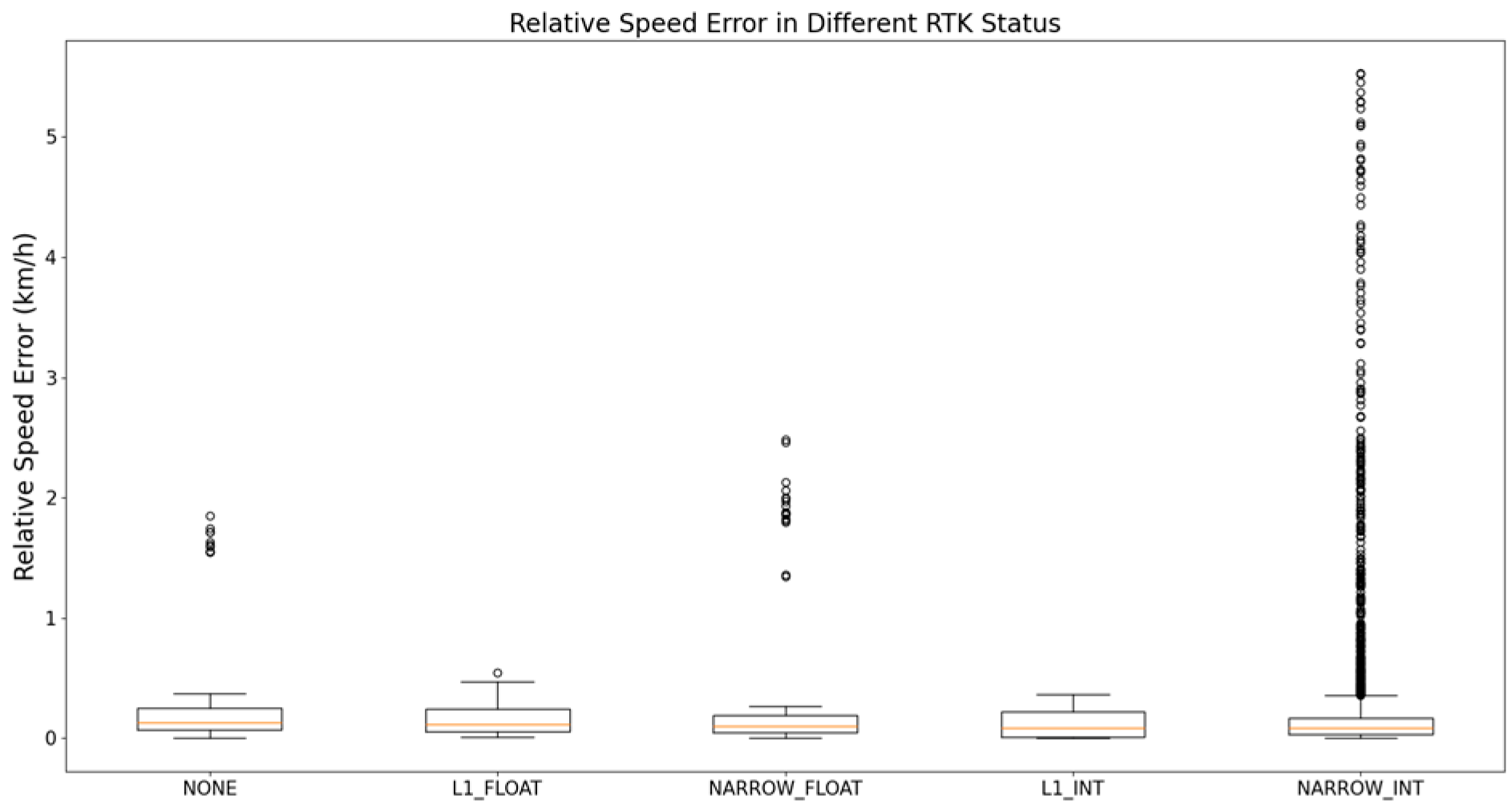
4.3. RTK Status Analysis

The performance of the MB-RTK framework is highly dependent on the RTK solution status, which directly affects relative positioning accuracy and stability. This section evaluates recovery time, relative distance error, and relative speed error under different RTK states to assess system robustness in dynamic scenarios.

Figure 12 illustrates the transition time from a non-RTK state to various RTK solutions. The results indicate that transitioning from ‘NONE → L1_FLOAT’ requires the longest recovery time (~20 s), whereas ‘NONE → NARROW_FLOAT’ and ‘NONE → NARROW_INT’ achieve significantly faster convergence. This suggests that direct transitions into high-precision states improve convergence efficiency.

Figure 13 and Figure 14 depict relative distance and speed variations across RTK states. The results show that NARROW_INT provides the most stable and accurate positioning, with minimal variance in distance and speed. In contrast, L1_FLOAT and NARROW_FLOAT exhibit greater fluctuations, indicating reduced stability. The NONE state results in the largest errors, confirming the necessity of continuous RTK corrections.

Figure 15 and Figure 16 further quantify relative distance and speed errors. NARROW_INT achieves the lowest errors, maintaining sub-10 m distance error and sub-0.1 km/h speed error. L1_INT also demonstrates high precision, while NARROW_FLOAT serves as a transitional state with moderate accuracy. The NONE state results in excessive errors, reinforcing the importance of stable RTK solutions in virtual coupling.

The performance differences across RTK modes are summarized in

Table 2. RTK performance metrics across different modes.

RTK Status	Recovery Time (s)	Distance Error (m)	Speed Error (km/h)
NONE	~20.0	>100	>1.0
L1_FLOAT	>10	50–100	0.5–1.0
NARROW_FLOAT	3–5	400–600	0.2–0.5
L1_INT	~5	10–50	0.1–0.3
NARROW_INT	5–8	<10	<0.1

. NARROW_INT ensures optimal positioning and velocity synchronization, making it the preferred mode for virtual coupling. L1_FLOAT and NARROW_FLOAT provide an intermediate trade-off between convergence time and accuracy. Maintaining stable RTK solutions is essential for precise spatiotemporal synchronization, with future improvements focusing on accelerating recovery and enhancing robustness against GNSS signal interruptions.

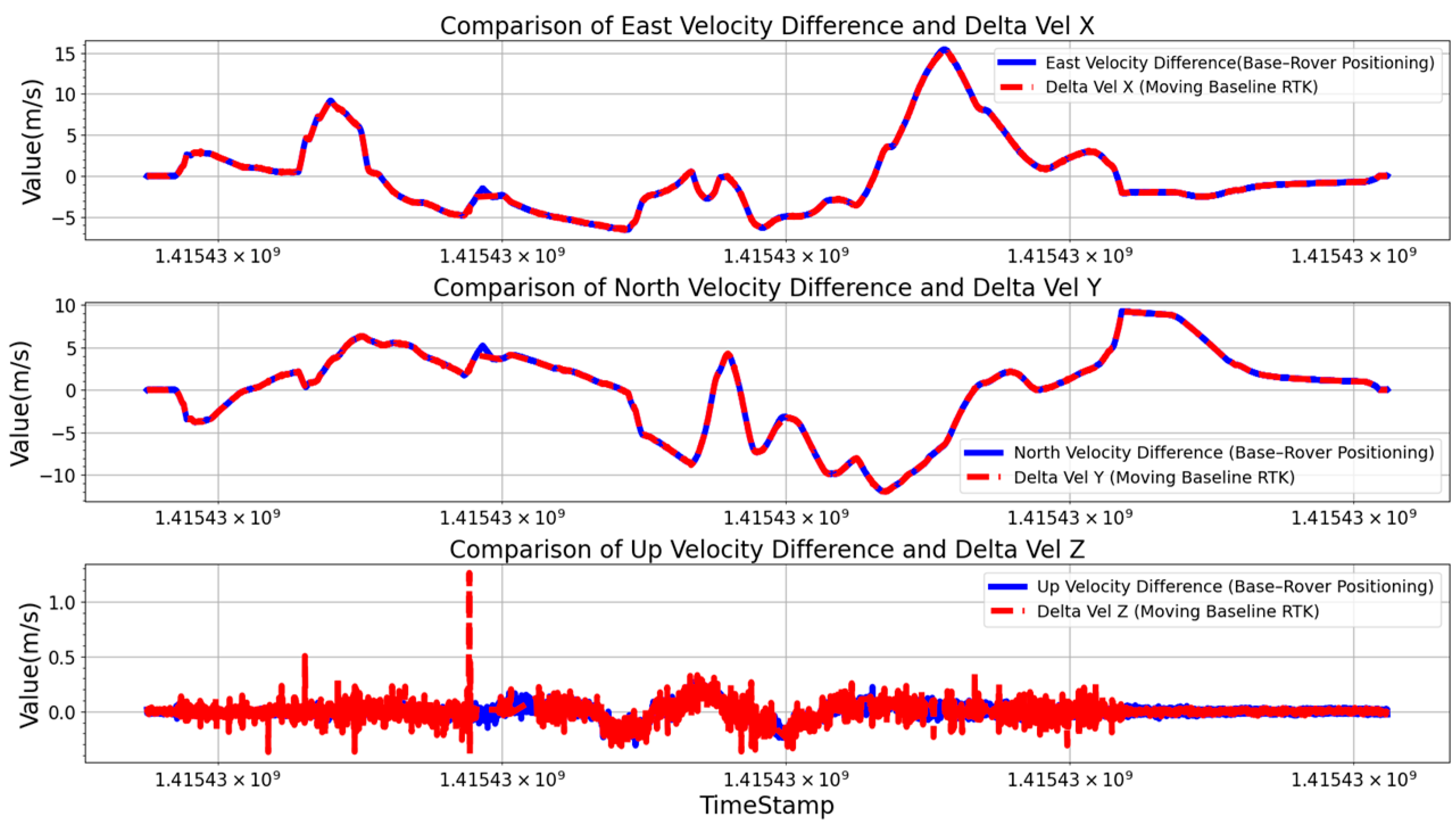
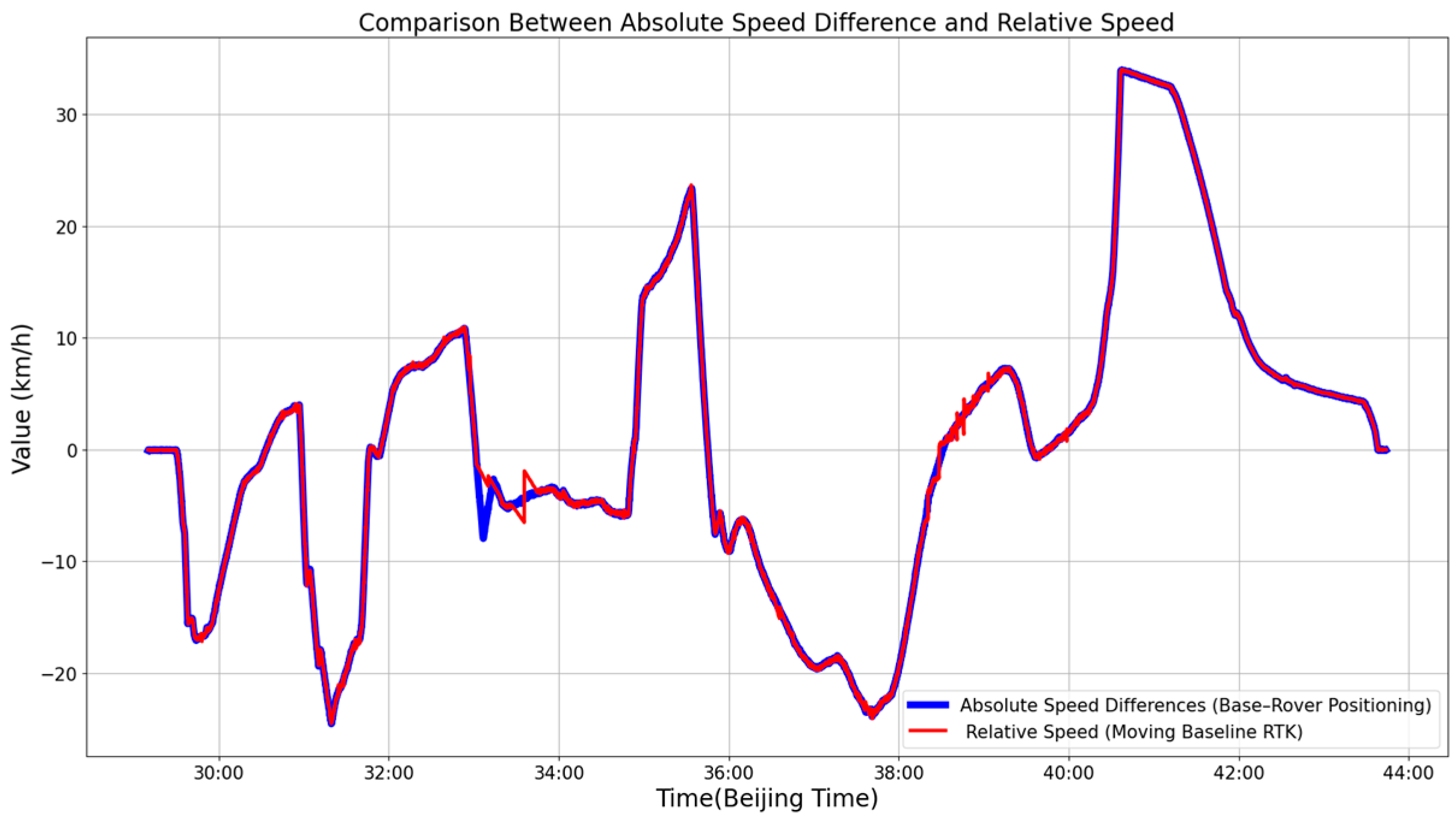
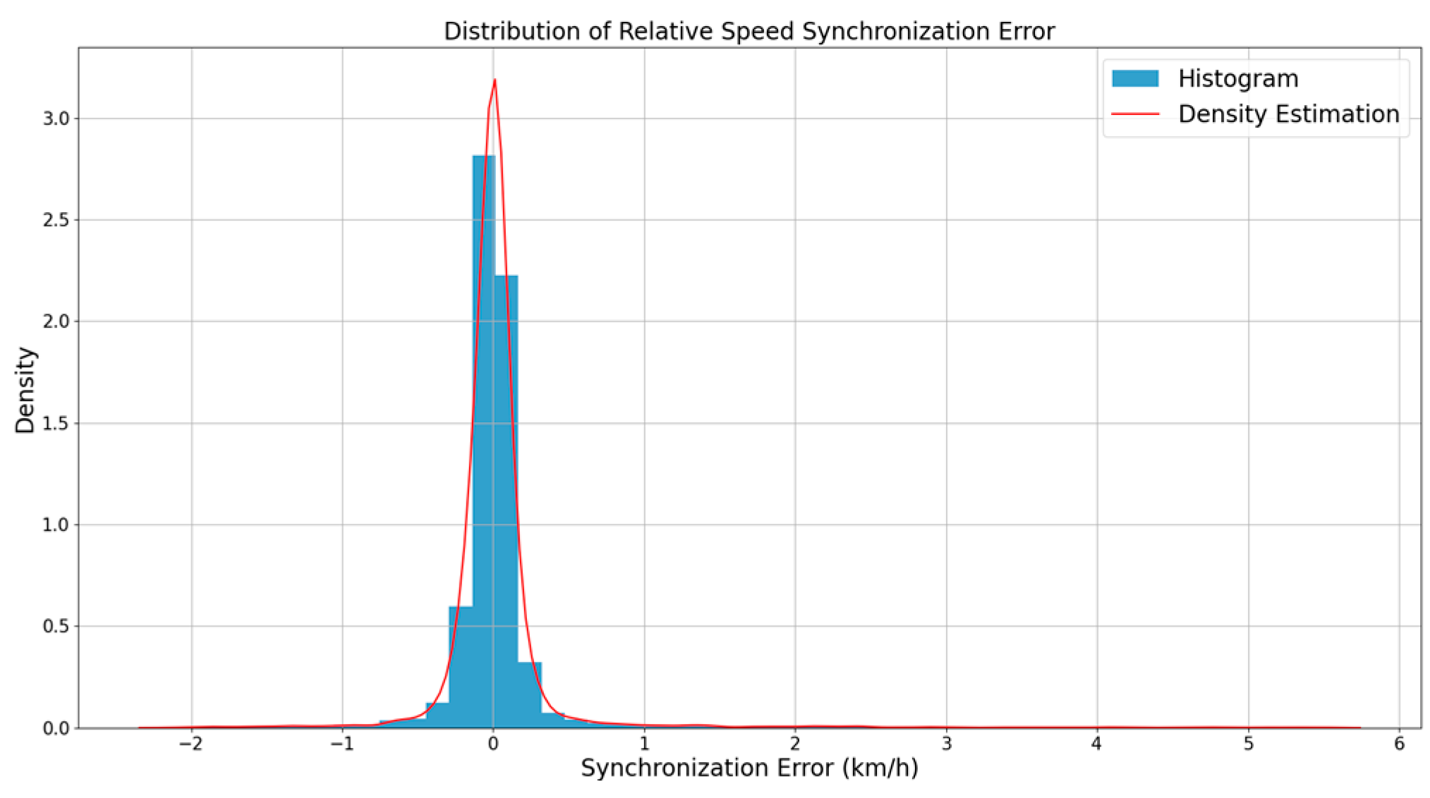
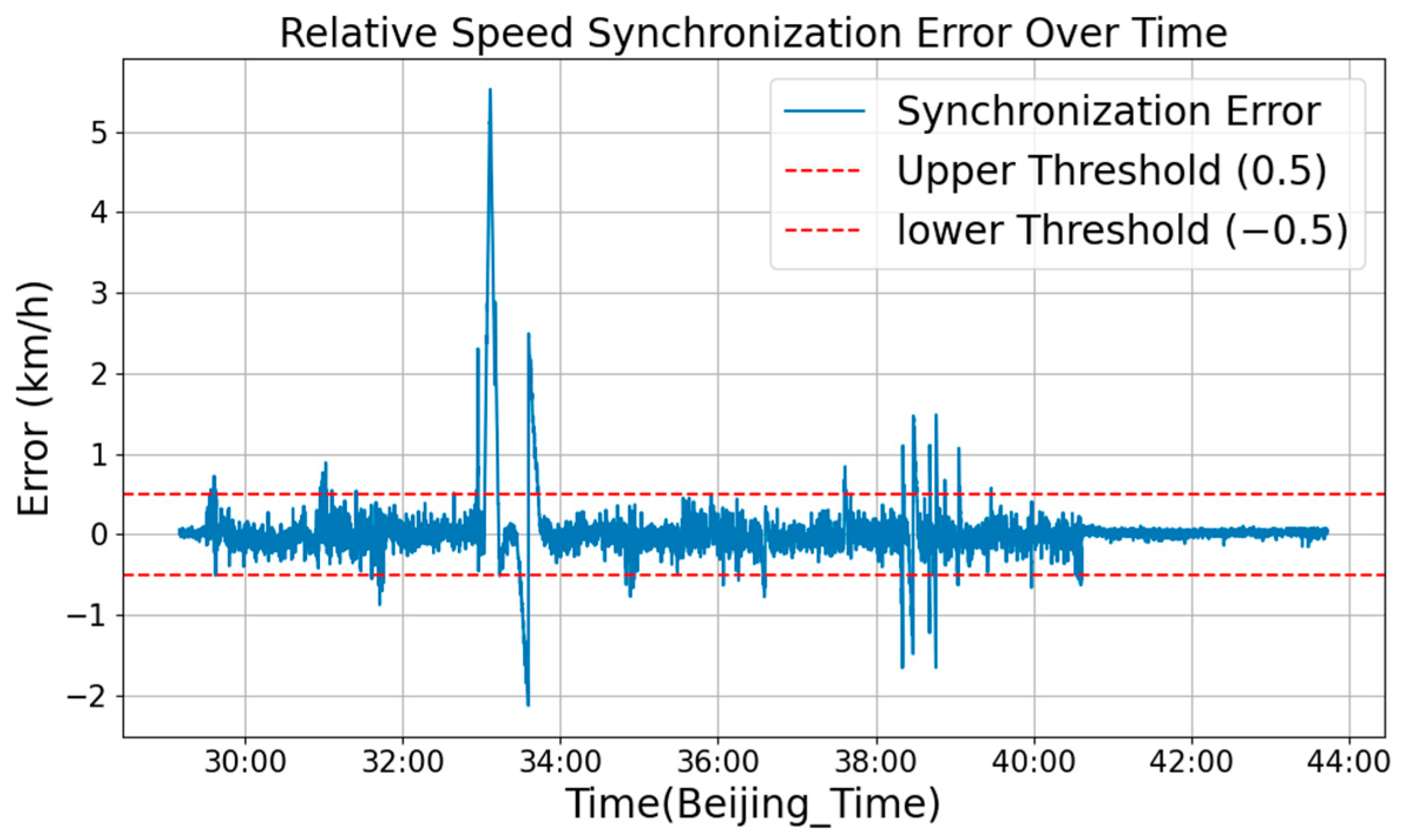
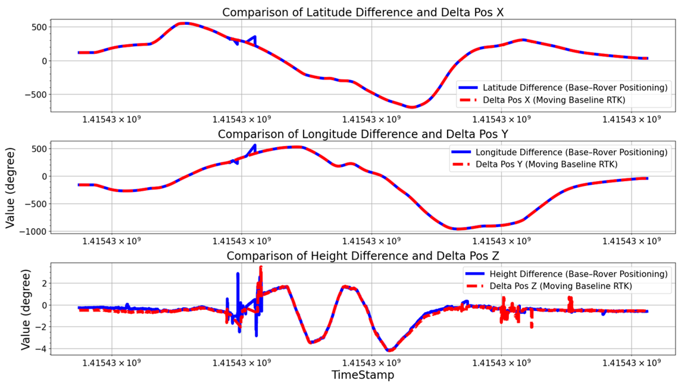
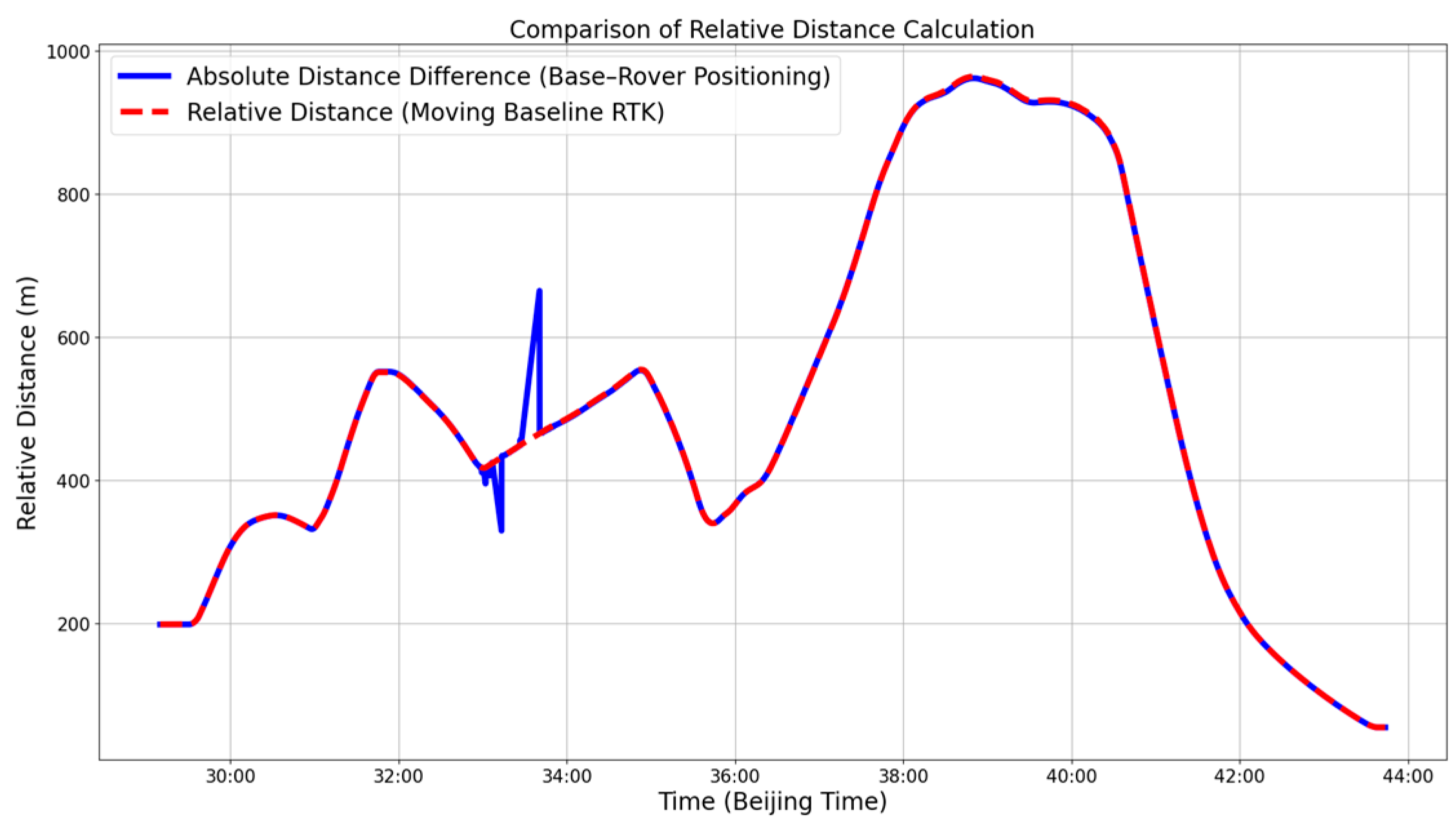
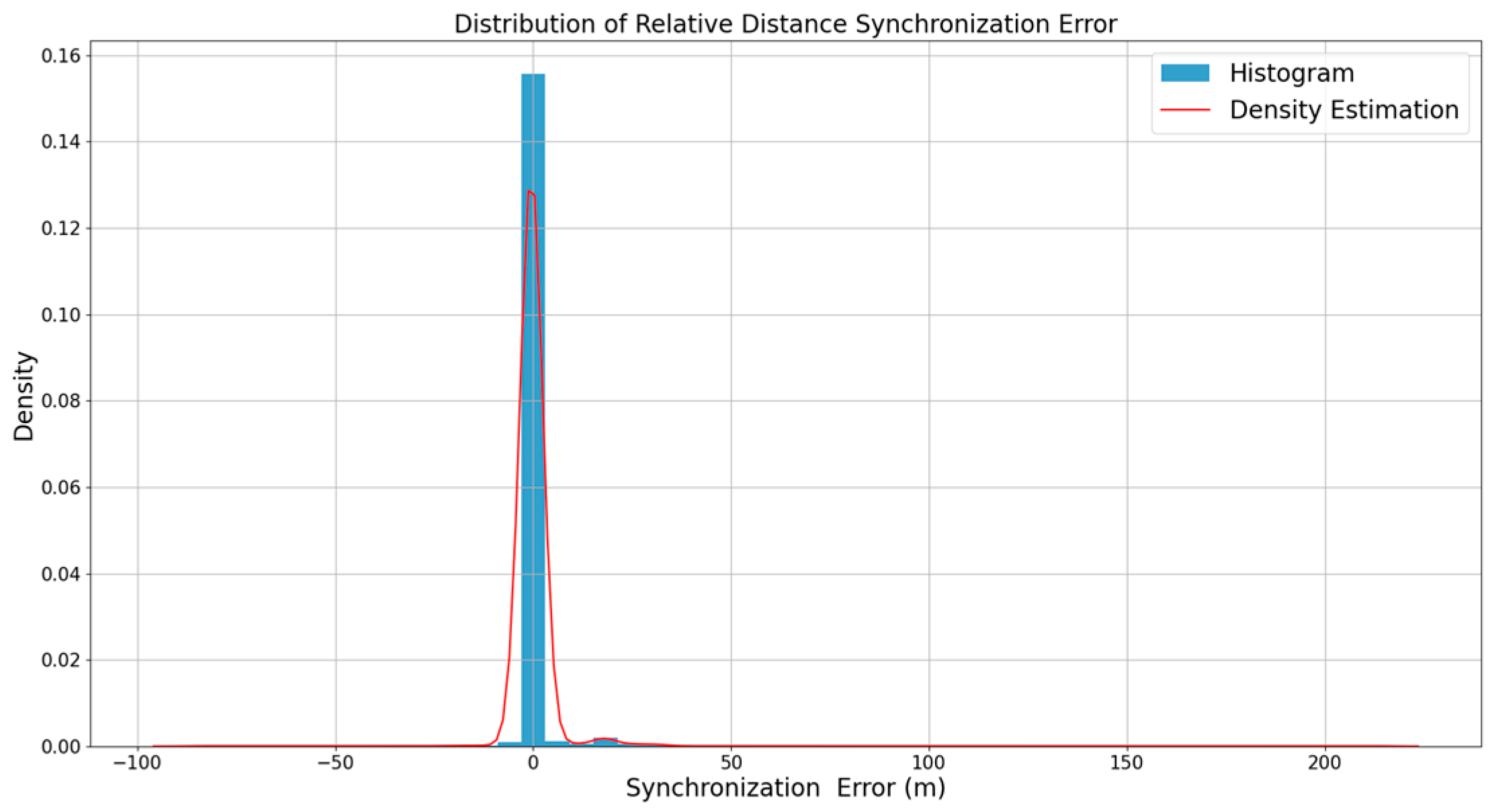
4.4. Spatiotemporal Synchronization Metrics

Figure 17 and Figure 18 compare absolute velocity difference (calculated from absolute GNSS positioning) with relative speed (derived from MB-RTK). The blue curve represents the absolute velocity difference, while the red curve shows the relative speed from MB-RTK. The two methods yield largely consistent results, confirming that MB-RTK provides reliable relative speed estimation. Figure 16 presents velocity errors in the ENU coordinate system, while Figure 18 compares absolute speed differences with MB-RTK-derived relative speed.

To quantify synchronization accuracy, Figure 19 provides a histogram and probability estimation of relative speed errors. The results show that most errors are concentrated around 0 km/h, demonstrating that MB-RTK effectively minimizes speed differences between coupled trains. In 95% of cases, errors remain within ±0.5 km/h, indicating high synchronization precision. Figure 20 further complements this analysis with a box plot of the same error distribution. The median synchronization error is approximately 0.02 km/h, and the interquartile range lies between −0.15 km/h and 0.18 km/h, indicating that the majority of errors are tightly clustered around zero.

However, occasional deviations up to 3 km/h are observed, particularly in areas with communication latency, GNSS signal jumps, or environmental interference. Figure 21 shows randomly varying relative speed errors, with occasional spikes—most notably around 32 min and 37 min—suggesting temporary disruptions in GNSS updates or sudden changes in motion state that MB-RTK fails to compensate for in real time.

MB-RTK achieves high speed synchronization accuracy, maintaining errors within ±0.5 km/h in most cases. However, occasional deviations up to 3 km/h highlight the need for improved robustness against GNSS signal loss and communication delays. Speed synchronization deviations may affect inter-train spacing, necessitating further optimization in extreme conditions to ensure safe virtual coupling operations.

Figure 22 and Figure 23 compare absolute position difference (calculated from GNSS absolute positioning) with relative distance (obtained from MB-RTK). The blue curve represents the relative distance derived from absolute positioning, while the red-dashed curve illustrates MB-RTK results. The close alignment of both curves confirms that MB-RTK provides highly accurate relative positioning, reducing fluctuations associated with absolute GNSS positioning. However, from 30:00 to 34:00, noticeable deviations occur, suggesting instability in absolute position estimates, while MB-RTK results remain smoother, demonstrating its robustness against GNSS signal loss and inertial navigation errors.

To quantify synchronization accuracy, Figure 24 presents a histogram and density estimation of relative distance errors. Results indicate that most errors are concentrated near 0, demonstrating high synchronization precision. A total of 90% of errors remain within ±10 m, confirming MB-RTK’s stability in maintaining inter-train distances.

Further analysis of error frequency components in Figure 25 reveals that low-frequency errors dominate, suggesting gradual variations due to environmental influences. In contrast, high-frequency fluctuations are minimal, indicating that MB-RTK effectively mitigates short-term motion disturbances.

Figure 26 applies a sliding mean and standard deviation control analysis to assess the temporal evolution of distance errors. The system maintains errors within ±10 m for most of the time, with a mean close to 0. However, during 33–35 min, error spikes are observed, likely due to GNSS signal degradation or base station switching, suggesting the need for further optimization in extreme scenarios.

MB-RTK ensures accurate inter-train relative positioning with minimal fluctuations. Most errors remain within ±10 m, but occasional spikes highlight the need for enhanced GNSS robustness. Maintaining precise distance synchronization is essential for safe virtual coupling operations, as distance fluctuations may affect train headway stability and safety margins. Further improvements should focus on mitigating GNSS signal loss effects to enhance system resilience. A detailed comparison between GNSS absolute methods and MB-RTK relative methods is presented in

Table 3. Comparison of GNSS absolute methods and MB-RTK relative methods.

Metric	GNSS Absolute Methods	MB-RTK Relative Methods
Relative speed accuracy	Highly affected by GNSS errors, leading to larger deviations	Lower errors, more stable speed fluctuations
Relative position accuracy	Higher errors, especially in long-span measurements	More stable, with errors concentrated near zero
Noise resistance	Prone to GNSS signal jumps and variations	Stronger resistance to noise and fluctuations
Adaptability to complex environments	Heavily influenced by multipath effects and signal loss	More robust against multipath interference and signal degradation

.

4.5. Summary

The experimental results confirm that MB-RTK significantly improves inter-train relative positioning, speed synchronization, and spatiotemporal consistency, making it well-suited for virtual coupling applications.

From the trajectory tracking analysis, MB-RTK maintains high-precision relative positioning, with deviations mostly within ±10 m. However, minor irregularities in distance tracking were observed, particularly during deceleration phases, indicating the need for enhanced robustness against GNSS signal fluctuations. The RTK status evaluation highlights that NARROW_INT provides the highest stability and accuracy, while L1_INT also offers reliable performance. Intermediate modes like NARROW_FLOAT and L1_FLOAT introduce moderate fluctuations, whereas the NONE mode results in excessive errors, making continuous RTK corrections essential for reliable virtual coupling. The synchronization metrics indicate that MB-RTK maintains speed deviations within ±0.5 km/h, ensuring smooth train coordination. However, momentary synchronization errors were detected during GNSS dropouts or sudden velocity changes, suggesting a need for adaptive correction mechanisms.

To address GNSS signal loss scenarios, such as in tunnels or urban environments with high-rise obstructions, an auxiliary sensor-based backup strategy is integrated into the system. When GNSS data are temporarily unavailable, the train relies on inertial measurement unit (IMU) and odometry sensors as alternative data sources for relative positioning. Specifically, during short-term GNSS outages, the system seamlessly transitions to an IMU-based dead reckoning mode, continuously estimating the relative position between coupled trains. Simultaneously, inter-train communication enables odometry-based corrections, where distance data shared between trains are used to refine the estimated trajectory and mitigate drift errors. These strategies ensure that virtual coupling remains stable even during transient GNSS interruptions. Furthermore, this solution serves as a critical mechanism in virtual coupling control but must be integrated with conventional train safety protection systems. In the event of prolonged GNSS unavailability, the system is designed to automatically increase the inter-train distance or transition to a conventional operation mode, ensuring fail-safe performance. This adaptive switching mechanism balances the benefits of high-precision positioning with operational safety, making MB-RTK more resilient in complex railway environments.

Overall, MB-RTK outperforms GNSS absolute positioning, offering greater accuracy, robustness, and synchronization reliability. However, RTK stability and real-time GNSS variations remain as challenges, warranting further improvements in error mitigation and adaptive synchronization strategies for enhanced performance in complex railway environments.

5. Conclusions

This paper introduced a high-accuracy MB-RTK framework for achieving robust spatiotemporal synchronization in virtual coupling systems. By leveraging GNSS carrier-phase differential processing and dynamic baseline estimation, MB-RTK enables precise inter-train relative positioning and velocity synchronization, ensuring stable and efficient convoy operations. Experimental validation demonstrated that the proposed approach can significantly enhance inter-train coordination, reduce headways, and improve system efficiency, making it a compelling solution for future railway networks.

The results underscore the importance of accurate spatiotemporal synchronization in VC applications. MB-RTK effectively mitigates GNSS-induced positioning errors; ensures low-latency synchronization; and improves the stability of train formations, particularly under challenging conditions. The findings suggest that MB-RTK, when combined with robust communication protocols and predictive control strategies, can further enhance synchronization reliability, making it well-suited for high-density and autonomous railway operations.

Despite its advantages, further research is needed to validate MB-RTK under more challenging terrains and climate conditions, such as mountainous railway networks and extreme weather scenarios, where GNSS signals may experience severe degradation. Additionally, when extending the proposed method to multi-train platooning, it is crucial to account for cumulative errors in vehicle-to-vehicle (V2V) chain communication. Communication delays can directly impact synchronization accuracy and safety, making latency-aware safety mechanisms a key focus in future research. Furthermore, for railway applications, the impact of track curvature on antenna vector length should be carefully analyzed, as variations in the baseline geometry due to track curvature may introduce additional localization errors.

In conclusion, MB-RTK provides a highly accurate, low-latency, and robust solution for train virtual coupling, offering safe, efficient, and flexible train coordination. Future research should focus on enhancing synchronization resilience, addressing communication-induced safety concerns, and refining localization accuracy under dynamic track conditions to further expand MB-RTK applications in next-generation railway automation.

References

1. Félez, J.; Vaquero-Serrano, M.A. Virtual Coupling in Railways: A Comprehensive Review. Machines 2023, 11, 521. [Google Scholar] [CrossRef]
2. X2Rail-3. Advanced Signalling, Automation and Communication System (IP2 and IP5)—Prototyping the Future by Means of Capacity Increase, Autonomy and Flexible Communication. Cordis Database. Available online: https://cordis.europa.eu/project/id/826141 (accessed on 7 October 2022).
3. Aoun, J.; Quaglietta, E.; Goverde, M.P. Roadmap Development for the Deployment of Virtual Coupling in Railway Signalling. Technol. Forecast. Soc. Chang. 2023, 189, 122263. [Google Scholar] [CrossRef]
4. Schumann, T. Increase of capacity on the shinkansen high-speed line using virtual coupling. Int. J. Transp. Dev. Integr. 2017, 1, 666–676. [Google Scholar] [CrossRef]
5. Liu, C.; Xu, Z. Multi-Agent System Based Cooperative Control for Speed Convergence of Virtually Coupled Train Formation. Sensors 2024, 24, 4231. [Google Scholar] [CrossRef]
6. Zhou, Y.; Chen, Q.; Wang, R.; Jia, G.; Niu, X. Onboard train localization based on railway track irregularity matching. IEEE Trans. Instrum. Meas. 2022, 71, 9501013. [Google Scholar] [CrossRef]
7. Li, G.; Zou, J.; Ma, W.; Lan, M. Research on virtual coupling technology in rail transit train collision protection. Transp. Saf. Environ. 2024, 6, tdad012. [Google Scholar] [CrossRef]
8. Park, J.; Lee, B.-H.; Eun, Y. Virtual Coupling of Railway Vehicles: Gap Reference for Merge and Separation, Robust Control, and Position Measurement. IEEE Trans. Intell. Transp. Syst. 2022, 23, 1085–1096. [Google Scholar] [CrossRef]
9. Quaglietta, E.; Spartalis, P.; Wang, M.; Goverde, R.M.; van Koningsbruggen, P. Modelling and analysis of Virtual Coupling with dynamic safety margin considering risk factors in railway operations. J. Rail Transp. Plan. Manag. 2022, 22, 100313. [Google Scholar] [CrossRef]
10. Tian, S.; Yan, F.; Shang, W.-L.; Majumdar, A.; Chen, H.; Chen, M.; Zeinab, M.; Tian, Y. Energy consumption analysis of trains based on multi-mode virtual coupling operation control strategies. Appl. Energy 2025, 377, 124684. [Google Scholar] [CrossRef]
11. Basile, G.; Lui, D.G.; Petrillo, A.; Santini, S. Deep deterministic policy gradient virtual coupling control for the coordination and manoeuvring of heterogeneous uncertain nonlinear high-speed trains. Eng. Appl. Artif. Intell. 2024, 133, 108120. [Google Scholar] [CrossRef]
12. Zhang, Q.; Wang, H.; Zhang, Y.; Chai, M.; Ma, S. An adaptive safety control approach for virtual coupling system with model parametric uncertainties. Transp. Res. Part C Emerg. Technol. 2023, 154, 104235. [Google Scholar] [CrossRef]
13. Cai, B.; Liu, J.; Dong, X.; Liu, J. Study on key technologies of GNSS-based train state perception for train-centric railway signaling. High-Speed Railw. 2023, 1, 47–55. [Google Scholar] [CrossRef]
14. Dong, Y.; Zhang, L.; Wang, D.; Li, Q.; Wu, J.; Wu, M. Low-latency, high-rate, high-precision relative positioning with moving base in real time. GPS Solut. 2020, 24, 56. [Google Scholar] [CrossRef]
15. Amatetti, C.; Polonelli, T.; Masina, E.; Moatti, C.; Mikhaylov, D.; Amato, D.; Vanelli-Coralli, A.; Magno, M.; Benini, L. Towards the Future Generation of Railway Localization and Signaling Exploiting sub-meter RTK GNSS. In Proceedings of the 2022 IEEE Sensors Applications Symposium (SAS), Sundsvall, Sweden, 1–3 August 2022; pp. 1–6. [Google Scholar] [CrossRef]
16. Yang, H.; Dong, S.-Q.; Xie, C.-H. High-speed train positioning based on a combination of Beidou navigation, inertial navigation and an electronic map. Sci. China Inf. Sci. 2023, 66, 172207. [Google Scholar] [CrossRef]
17. Mikhaylov, D.; Amatetti, C.; Polonelli, T.; Masina, E.; Campana, R.; Berszin, K.; Moatti, C.; Amato, D.; Vanelli-Coralli, A.; Magno, M.; et al. Toward the Future Generation of Railway Localization Exploiting RTK and GNSS. IEEE Trans. Instrum. Meas. 2023, 72, 8502610. [Google Scholar] [CrossRef]
18. Specht, M.; Specht, C.; Stateczny, A.; Burdziakowski, P.; Dąbrowski, P.; Lewicka, O. Study on the positioning accuracy of the GNSS/INS system supported by the RTK receiver for railway measurements. Energies 2022, 15, 4094. [Google Scholar] [CrossRef]
19. Jiang, W.; Liu, Y.; Li, J.; Wang, J.; Rizos, C.; Cai, B. Robust train length calculation and monitoring method using GNSS multi-constellation moving-baseline positioning resolution. GPS Solut. 2024, 28, 114. [Google Scholar] [CrossRef]
20. Wang, S.; Dai, P.; Xu, T.; Nie, W.; Cong, Y.; Xing, J.; Gao, F. Maximum Mixture Correntropy Criterion-Based Variational Bayesian Adaptive Kalman Filter for INS/UWB/GNSS-RTK Integrated Positioning. Remote Sens. 2025, 17, 207. [Google Scholar] [CrossRef]
21. Schutz, A.; Sanchez-Morales, D.E.; Pany, T. Precise positioning through a loosely-coupled sensor fusion of GNSS-RTK, INS and LiDAR for autonomous driving. In Proceedings of the IEEE/ION Position, Location and Navigation Symposium (PLANS), Portland, OR, USA, 20–23 April 2020; pp. 219–225. [Google Scholar] [CrossRef]
22. Ji, S.; Wang, J.; Weng, D.; Chen, W. Detailed Investigation on Ambiguity Validation of Long-Distance RTK. Remote Sens. 2024, 16, 2982. [Google Scholar] [CrossRef]
23. Huang, W.; Zhao, Z.; Zhu, X. An Effective Scheme for Modeling and Compensating Differential Age Errors in Real-Time Kinematic Positioning. Remote Sens. 2024, 16, 2662. [Google Scholar] [CrossRef]
24. Elsayed, H.; El-Mowafy, A.; Allahvirdi-Zadeh, A.; Wang, K.; Mi, X. A Combination of Classification Robust Adaptive Kalman Filter with PPP-RTK to Improve Fault Detection for Integrity Monitoring of Autonomous Vehicles. Remote Sens. 2025, 17, 284. [Google Scholar] [CrossRef]
25. Han, J.-H.; Park, C.-H.; Jang, Y.Y. Development of a Moving Baseline RTK/Motion Sensor-Integrated Positioning-Based Autonomous Driving Algorithm for a Speed Sprayer. Sensors 2022, 22, 9881. [Google Scholar] [CrossRef] [PubMed]
26. Kazim, S.A.; Tmazirte, N.A.; Marais, J. Realistic position error models for GNSS simulation in railway environments. In Proceedings of the European Navigation Conference (ENC), Dresden, Germany, 23–24 November 2020; pp. 1–9. [Google Scholar] [CrossRef]
27. Shehata, A.G.; Zarzoura, F.H.; El-Mewafi, M. Assessing the influence of differential code bias and satellite geometry on GNSS ambiguity resolution through MANS-PPP software package. J. Appl. Geodesy 2023, 18, 1–20. [Google Scholar] [CrossRef]
28. Jia, M.; Khalife, J.; Kassas, Z.M. Performance analysis of opportunistic ARAIM or navigation with GNSS signals fused with terrestrial signals of opportunity. IEEE Trans. Intell. Transp. Syst. 2023, 24, 10587–10602. [Google Scholar] [CrossRef]
29. Guo, W.; Li, L.; Zhao, D.; Zhu, F.; Lai, L. Enhancing BDS-3 PPP-B2b real-time positioning performance by tightly integrating MEMS IMU and LiDAR in GNSS-degraded environment. Measurement 2025, 242, 116015. [Google Scholar] [CrossRef]
30. Xiao, S.; Ge, X.; Wu, Q.; Ding, L. Co-design of bandwidth-aware communication scheduler and cruise controller for multiple high-speed trains. IEEE Trans. Veh. Technol. 2024, 73, 4993–5004. [Google Scholar] [CrossRef]
31. Zeng, P.; Zhang, Y.; Xia, X.; Zhang, J.; Du, P.; Hua, Z.; Li, S. Research on sea clutter simulation method based on deep cognition of characteristic parameters. Remote Sens. 2024, 16, 4741. [Google Scholar] [CrossRef]
32. Wu, Q.; Ge, X.; Zhu, S.; Cole, C.; Spiryagin, M. Physical coupling and decoupling of railway trains at cruising speeds: Train control and dynamics. Int. J. Rail Transp. 2023, 12, 217–232. [Google Scholar] [CrossRef]
33. Schenker, M. S2R Innovation Days Presentation X2R3-TD2.8 Virtually Coupled Train Sets. In Proceedings of the S2R Innovation Days Presentation X2R3-TD2.8 Virtually Coupled Train Sets, Stuttgart, Germany, 22–23 October 2020. [Google Scholar]
Figure 1. System architecture.
Remotesensing 17 01238 g001
Figure 2. Comparison of traditional braking model and virtual coupling braking model.
Remotesensing 17 01238 g002
Figure 3. Comparison between ABD and RBD for four different railway scenarios [33].
Remotesensing 17 01238 g003
Figure 4. Schematic diagram of the moving baseline solution process.
Remotesensing 17 01238 g004
Figure 5. Closed-loop experimental line.
Remotesensing 17 01238 g005
Figure 6. The leading train.
Remotesensing 17 01238 g006
Figure 7. The following train.
Remotesensing 17 01238 g007
Figure 8. GNSS receiver in driver’s cab.
Remotesensing 17 01238 g008
Figure 9. Two train running trajectory.
Remotesensing 17 01238 g009
Figure 10. Base station and rover station running speed over time.
Remotesensing 17 01238 g010
Figure 11. Base station and rover station running distance over time.
Remotesensing 17 01238 g011
Figure 12. RTK status recovery time (seconds).
Remotesensing 17 01238 g012
Figure 13. Relative distance distribution by RTK status.
Remotesensing 17 01238 g013
Figure 14. Relative speed peed distribution by RTK status.
Remotesensing 17 01238 g014
Figure 15. Relative distance error (Base-Rover and MB-RTK) by RTK status.
Remotesensing 17 01238 g015
Figure 16. Relative speed error (Base-Rover and MB-RTK) by RTK status.
Remotesensing 17 01238 g016
Figure 17. Comparison between absolute velocity differences (Base–Rover Positioning, ENU) and relative velocity (MB-RTK, XYZ).
Remotesensing 17 01238 g017
Figure 18. Comparison between absolute speed difference (Base–Rover Positioning) and relative speed (MB-RTK).
Remotesensing 17 01238 g018
Figure 19. Distribution of relative speed synchronization error (histogram and density estimation).
Remotesensing 17 01238 g019
Figure 20. Box plot of relative speed synchronization error.
Remotesensing 17 01238 g020
Figure 21. Relative speed synchronization error over time.
Remotesensing 17 01238 g021
Figure 22. Comparison between absolute position difference (Base–Rover Positioning, ENU) and relative position (MB-RTK, XYZ).
Remotesensing 17 01238 g022
Figure 23. Comparison between absolute distance difference (Base–Rover Positioning) and relative distance (MB-RTK).
Remotesensing 17 01238 g023
Figure 24. Distribution of relative distance synchronization error (histogram and density estimation).
Remotesensing 17 01238 g024
Figure 25. Wavelet analysis of relative distance synchronization error.
Remotesensing 17 01238 g025
Figure 26. Relative distance synchronization error with statistical control and moving statistics.
Remotesensing 17 01238 g026