Two-Dimensional Spatial Variation Analysis and Correction Method for High-Resolution Wide-Swath Spaceborne Synthetic Aperture Radar (SAR) Imaging

Abstract

With the development and application of spaceborne Synthetic Aperture Radar (SAR), higher resolution and a wider swath have become significant demands. However, as the resolution increases and the swath widens, the two-dimensional (2D) spatial variation between different targets in the scene and the radar becomes very pronounced, severely affecting the high-precision focusing and high-quality imaging of spaceborne SAR. In previous studies on the correction of two-dimensional spatial variation in spaceborne SAR, either the models were not accurate enough or the computational efficiency was low, limiting the application of corresponding algorithms. In this paper, we first establish a slant range model and a signal model based on the zero-Doppler moment according to the spaceborne SAR geometry, thereby significantly reducing the impact of azimuth spatial variation in two-dimensional spatial variation. Subsequently, we propose a Curve-Sphere Model (CUSM) to describe the ground observation geometry of spaceborne SAR, and based on this, we establish a more accurate theoretical model and quantitative description of two-dimensional spatial variation. Next, through modeling and simulation, we conduct an in-depth analysis of the impact of two-dimensional spatial variation on spaceborne SAR imaging, obtaining corresponding constraints and thresholds and concluding that in most cases, only one type of azimuth spatial variation needs to be considered, thereby greatly reducing the demand and difficulty of two-dimensional spatial variation correction. Relying on these, we propose a two-dimensional spatial variation correction method that combines range blocking and azimuth nonlinear chirp scaling processing and analyze its scalability to be applicable to more general cases. Finally, the effectiveness and applicability of the proposed method are validated through both simulation experiments and real data experiments.

1. Introduction

Spaceborne SAR has long garnered extensive attention and in-depth research due to its all-weather and all-day observation capabilities [1,2,3,4,5,6,7,8,9,10]. With the increasing application demands in both the military and civilian fields, higher resolution and larger mapping bandwidth have become important development directions for spaceborne SAR. In recent years, many spaceborne SAR systems have achieved decimeter-level resolution capabilities [11,12], with the Capella-9 and Capella-10 satellites even reaching centimeter-level theoretical resolution capabilities in the azimuth dimension [13].

However, as the resolution increases and the observation range expands, a scenario generally referred to as High Resolution, Wide Swath (HRWS), the difficulty of precise imaging for spaceborne SAR also gradually increases. On one hand, higher resolution implies lower error tolerance, necessitating the use of more accurate geometric and signal models. On the other hand, in the case of high resolution, a larger observation range will make the effects of spatial variation more severe, and this spatial variation exists in both the range and azimuth dimensions, thus requiring the consideration of two-dimensional spatial variation.

In HRWS spaceborne SAR, the sources of two-dimensional spatial variation mainly stem from three aspects. First, as the synthetic aperture increases, the satellite trajectory over the entire imaging time cannot be approximated by a straight line, and the satellite’s velocity is no longer constant. Second, with the increase in imaging time, the Earth’s rotation must be taken into account, which causes the satellite trajectory to become a non-coplanar curved line in the Earth-Centered, Earth-Fixed (ECEF) coordinate system. Third, as the observation range expands, the curvature of the Earth’s surface also needs to be considered, leading to higher-order characteristics in the two-dimensional spatial variation, especially in the variation in spatial range.

The development of spaceborne SAR imaging algorithms has always been accompanied by research on the analysis and correction methods of two-dimensional spatial variation. In fact, if imaging efficiency is not considered, time-domain imaging algorithms such as the back-projection algorithm (BPA) can effectively address the issue of two-dimensional spatial variation. However, in the HRWS scenario, the data volume is so large that even the optimized and accelerated BPA remains highly inefficient. Therefore, frequency-domain algorithms that can balance imaging quality and computational efficiency have become a continuous exploration goal.

In early studies, due to the lower resolution, spaceborne SAR could often be processed using the geometric model of airborne SAR, thereby neglecting the azimuth spatial variation issues inherent in spaceborne SAR and only considering the impact of spatial range variation. However, with the improvement in resolution, the increase in synthetic aperture length necessitates the consideration of azimuth spatial variation effects in spaceborne SAR imaging. Traditional algorithms such as the chirp scaling algorithm (CSA), the range-Doppler algorithm (RDA), and the omega-K algorithm ($\omega$KA) are no longer applicable.

Subsequently, a large number of studies on the azimuth spatial variation problem of spaceborne SAR have been conducted, and many imaging algorithms have been proposed, but the imaging results are not very satisfactory. Reference [14] divides the full aperture into several sub-apertures to ensure that there is no azimuth spatial variation within a sub-aperture, but the data stitching problem of sub-apertures is very challenging. References [15,16] achieve full-aperture imaging based on sub-aperture correction preprocessing and azimuth resampling, but their signal models still rely on the inaccurate assumption that the radar moves along a straight line. References [17,18] implement two-dimensional spatial variation decoupling to remove azimuth spatial variation based on time-domain and frequency-domain resampling (interpolation) processing, but the computational load of resampling (interpolation) is very large, and the interpolation accuracy is limited by the length of the interpolation kernel.

In recent years, several more precise imaging algorithms have been proposed to accommodate higher resolution and larger swathes. Reference [9] introduced a method that involves coarse imaging first, followed by blocking and iterative imaging, and finally, the fine imaging of small blocks that no longer have spatial variation. Although the algorithm is conceptually simple, it effectively addresses the two-dimensional spatial variation problem, and the increased computational load is still much smaller than that of BPA. However, this algorithm does not provide a basis for block segmentation, the iterative method lacks a clear termination condition, and the efficiency is relatively low. Reference [10] proposed an imaging algorithm based on spherical geometry, which corrects the actual satellite trajectory to a circle rather than a straight line, as is the case in most of the literature, thereby achieving two-dimensional spatial variation correction through motion compensation. However, this algorithm requires two-dimensional interpolation, has low efficiency, and approximates the Earth as a perfect sphere.

In summary, there is almost no literature that provides precise qualitative analysis and quantitative description of the two-dimensional spatial variation characteristics of HRWS spaceborne SAR, and there is also no algorithm that can simply and efficiently remove the two-dimensional spatial variation to achieve accurate focusing.

Therefore, this paper first conducts an in-depth analysis of the two-dimensional spatial variation based on the spaceborne SAR imaging geometry and establishes a quantitative description model. Subsequently, the two-dimensional spatial variation correction is achieved based on range blocking and azimuth nonlinear chirp scaling (NCS) processing without the need for any interpolation or iterative processing. The remainder of this paper is organized as follows: Section 2 establishes the spaceborne SAR geometric model and signal model; Section 3 provides a thorough theoretical analysis of the two-dimensional spatial variation in HRWS spaceborne SAR and establishes a quantitative description; Section 4 details the impact of two-dimensional spatial variation on imaging and identifies the constraints of these effects; Section 5 proposes a two-dimensional spatial variation correction method based on range blocking and azimuth NCS and discusses its extensibility; Section 6 demonstrates the algorithm’s effectiveness through both simulation experiments and real data validation; and Section 7 concludes the paper.

2. Geometric and Signal Models of Spaceborne SAR

SAR achieves high-resolution imaging capability through the relative motion between the radar and targets. To obtain higher resolution within the same imaging time duration, azimuth beam scanning is often required, i.e., operating in spotlight or sliding mode. To maximize the range swath width, azimuth multi-channel antenna configurations are typically employed. Since azimuth multi-channel processing falls beyond the scope of this paper, we neglect the errors introduced by this processing and assume the received signal can be equivalent to a single-channel received signal, whose Pulse Repetition Frequency (PRF) already satisfies the imaging requirements for SAR beam scanning modes.

When the radar transmits a linear frequency-modulated (LFM) signal, and under the “stop-and-go” assumption, for a ground point target $P\left(R_0,t_p\right)$, the received signal after quadrature demodulation can be expressed as

$$\begin{array}{cc}\hfill & s{s}_{receive}\left(t_r,t_a;R_0,t_p\right)=w_r\left[t_r-{\displaystyle \frac{2R\left(t_a;R_0,t_p\right)}{c}}\right]w_a\left(t_a-t_c\right)\hfill \\ & \times \sigma \left(R_0,t_p\right)exp\left\{-j4\pi {\displaystyle \frac{R\left(t_a;R_0,t_p\right)}{\lambda }}\right\}exp\left\{j\pi K_r{\left[t_r-{\displaystyle \frac{2R\left(t_a;R_0,t_p\right)}{c}}\right]}^2\right\}\hfill \end{array}$$

(1)

where $\lambda$ is the wavelength; c is the speed of light; $K_r$ is the transmit signal chirp rate; $t_r$ and $t_a$ represent the fast time and slow time, respectively; $w_r$ and $w_a$ are the range and azimuth window functions; and $t_p$ and $R_0$ denote the zero-Doppler time and corresponding slant range of point target P. $R(t_a;R_0,t_p)$ represents the slant range history between the radar and target P, $\sigma \left(R_0,t_p\right)$ represents the Radar Cross-Section (RCS) of Point Target P. The azimuth time instant $t_c$ corresponds to the moment when the beam center illuminates Target P, which arises from variations in the azimuth beam direction. The observation geometry of spaceborne SAR is illustrated in Figure 1 (taking the sliding spotlight mode as a representative example).

In Equation (1), the slant range history $R\left(t_a;R_0,t_p\right)$ has the most significant impact on subsequent focusing processing, and thus, its precise description directly affects imaging quality. In early literature, the slant range history model was typically modified based on the hyperbolic model, but its essence still relied on the premise of linear satellite motion. For HRWS scenarios, satellites can no longer be assumed to follow linear motion, and their curved trajectories must be considered. Therefore, recent literature generally establishes more precise slant range models using higher-order Taylor expansions and accordingly develops descriptive two-dimensional spatial variation equations.

It should be noted that many papers (such as [19,20]) expand the slant range history as a polynomial of $t_a-t_c$, thereby defining the two-dimensional spatial variation as functions of the azimuth beam center plane crossing time $t_c$ and the corresponding slant range $R_c$. However, this definition approach for two-dimensional spatial variation is insufficiently accurate. Figure 2a and Figure 2b, respectively, illustrate the intersection lines between the azimuth beam center plane and the observed scene in sliding spotlight mode and spotlight mode. The figures reveal that different targets sharing the same $t_c$ exhibit “tilted” spatial distributions within the scene, which will lead to severe azimuth spatial variation when using $t_c$ as the variable. Consequently, subsequent imaging processing becomes extremely challenging.

In this paper, we define two-dimensional spatial variation as functions of zero-Doppler time $t_p$ and closest slant range $R_0$. Targets sharing the same $t_p$ will be distributed along the red line shown in Figure 2c, thereby reducing azimuth spatial variation and facilitating precise imaging. Furthermore, describing targets and two-dimensional spatial variation using zero-Doppler time $t_p$ and closest slant range $R_0$ offers two additional advantages. First, the two-dimensional spatial variation originates solely from the geometric distribution of targets, independent of imaging modes. This interpretation better aligns with the fundamental definition of spatial variation and enables uniform processing across different imaging methods. Second, the imaged targets will be accurately compressed at position $\left(R_0,t_p\right)$, which better matches the geographic distribution of observation scenarios and eliminates the need for additional geometric distortion correction [21].

Figure 3 illustrates the target layout with a resolution of 0.5 × 0.5 m and an observation area of 10 × 10 km, with simulation parameters detailed in

Table 1. Simulation parameters of LEO spaceborne SAR.

Parameter	Value
Semi-major axis	6897.56 km
Orbital inclination	97.46°
Eccentricity	0.0013
Longitude of the ascending node	0°
Argument of periapsis	111.11°
True anomaly	0°
Look angle	25°
Wavelength	0.031 m

. The targets depicted in the figure are projections onto the Earth’s surface from three-dimensional space, centered around a reference target. The horizontal axis represents the azimuth position offset of the target relative to the reference target, while the vertical axis indicates the range position offset of the target relative to the reference target. (a) shows the target layout results based on the sliding-spotlight mode at the moment of beam center, (b) presents the target layout results based on the spotlight mode at the moment of beam center, and (c) depicts the target layout results for both sliding-spotlight mode and spotlight mode at zero-Doppler moments. The blue circles in the figure represent targets obtained from the sliding-spotlight mode, while the red stars represent targets obtained from the spotlight mode. The simulation results are consistent with the previous analysis.

In this paper, we first construct a slant range model based on the sixth-order Taylor expansion:

$$R\left(t_a;R_0,t_p\right)\approx R_0+\sum _{n=1}^6{k}_n{\left(t_a-t_p\right)}^n$$

(2)

where $k_n$ denotes the n-th order coefficient of $t_a-t_p$, and since $t_p$ represents the zero-Doppler time instant, $k_1$ is always zero and is thus neglected in subsequent derivations. In high-resolution spaceborne SAR operations, due to orbital curvature, Earth’s rotation, and Earth’s curvature, the expansion coefficients $k_n$ for different targets become functions of $R_0$ and $t_p$ (detailed descriptions and representations will be provided in the next section).

In most cases, a sixth-order model is sufficiently accurate, and the model order can be increased as needed without affecting subsequent analysis and processing workflows. Figure 4 shows the phase error between the sixth-order slant range model and the actual slant range, with the simulation parameters listed in Table 1. (a) presents the simulation results for an azimuth resolution of 0.2 m and an azimuth swath of 20 km, while (b) shows the simulation results for a resolution of 0.1 m and an azimuth swath of 10 km. Different lines represent different targets with the same closest slant range but different azimuth positions. As shown, the phase error of all of the targets are significantly below the threshold of 0.25$\pi$ [22].

By employing the series-inversion method, the corresponding two-dimensional spectrum of Equation (1) can be obtained. Neglecting amplitude and window function effects, it can be expressed as

$$\begin{array}{cc}\hfill & S{S}_{receive}\left(f_r,f_a;R_0,t_p\right)=exp\left(-j\pi {\displaystyle \frac{f_r^2}{K_r}}\right)exp\left(-j4\pi {\displaystyle \frac{f_c+f_r}{c}}{R}_0\right)\hfill \\ & \times exp\left(-j2\pi t_p{f}_a\right)exp\left(j\pi {\displaystyle \frac{c}{f_c+f_r}}{\displaystyle \frac{1}{4k_2}}{f}_a^2\right)exp\left(j\pi {\displaystyle \frac{c^2}{{\left(f_c+f_r\right)}^2}}{\displaystyle \frac{k_3}{16k_2^3}}{f}_a^3\right)\hfill \\ & \times exp\left(j\pi {\displaystyle \frac{c^3}{{\left(f_c+f_r\right)}^3}}{\displaystyle \frac{9k_3^2-4k_2{k}_4}{256k_2^5}}{f}_a^4\right)\hfill \\ & \times exp\left(j\pi {\displaystyle \frac{c^4}{{\left(f_c+f_r\right)}^4}}{\displaystyle \frac{27{k_3}^3-24k_2{k}_3{k}_4+4{k_2}^2{k}_5}{1024k_2^7}}{f}_a^5\right)\hfill \\ & \times exp\left(j\pi {\displaystyle \frac{c^5}{{\left(f_c+f_r\right)}^5}}{\displaystyle \frac{189{k_3}^4-252k_2{k_3}^2{k}_4+32{k_2}^2{k_4}^2+60{k_2}^2{k}_3{k}_5-8{k_2}^3{k}_6}{8192k_2^9}}{f}_a^6\right)\hfill \end{array}$$

(3)

By further organizing it as a function of range frequency, it can be expressed as

$$\begin{array}{cc}\hfill & S{S}_{receive}\left(f_r,f_a;R_0,t_p\right)=exp\left(-j\pi {\displaystyle \frac{f_r^2}{K_r}}\right)exp\left(-j4\pi {\displaystyle \frac{f_c+f_r}{c}}{R}_0\right)exp\left(-j2\pi t_p{f}_a\right)\hfill \\ & \times exp\left(j{\varphi }_0\left(f_a;R_0,t_p\right)\right)exp\left(j{\varphi }_1\left(f_a;R_0,t_p\right)f_r\right)exp\left(j{\varphi }_2\left(f_a;R_0,t_p\right)f_r^2\right)\hfill \\ & \times exp\left(j{\varphi }_3\left(f_a;R_0,t_p\right)f_r^3\right)exp\left(j\left({\sum }_{N>3}{\varphi }_N\left(f_a;R_0,t_p\right)f_r^N\right)\right)\hfill \end{array}$$

(4)

In Equation (4), the first exponential term represents the range modulation of the transmitted signal, the second exponential term denotes the phase information and range position of the target, the third exponential term indicates the azimuth position, the fourth exponential term represents the azimuth modulation, and the fifth exponential term accounts for the RCM. The sixth, seventh, and eighth exponential terms correspond to the second-order, third-order, and higher-order information of the range frequency, respectively. The specific expressions for ${\varphi }_0$, ${\varphi }_1$, ${\varphi }_2$, and ${\varphi }_3$ can be found in [22].

3. Theoretical Analysis of Two-Dimensional Spatial Variation

In Reference [22], we proposed the Circle-Sphere Model (CSM) to describe the observation geometry of spaceborne SAR and conducted a theoretical analysis of the spatial range variation based on this model. The CSM was derived under the assumption of no spatial azimuth variation, which remains applicable for high-resolution wide-swath scenarios with a 10 km swath width and a 0.2 m resolution. However, as the resolution further increases and the swath width further expands, the CSM will no longer be applicable. Therefore, in this paper, we first establish a more generalized spaceborne SAR geometric model, the Curve-Sphere Model (CUSM), and subsequently perform theoretical analysis and provide a quantitative description of two-dimensional spatial variation based on this model.

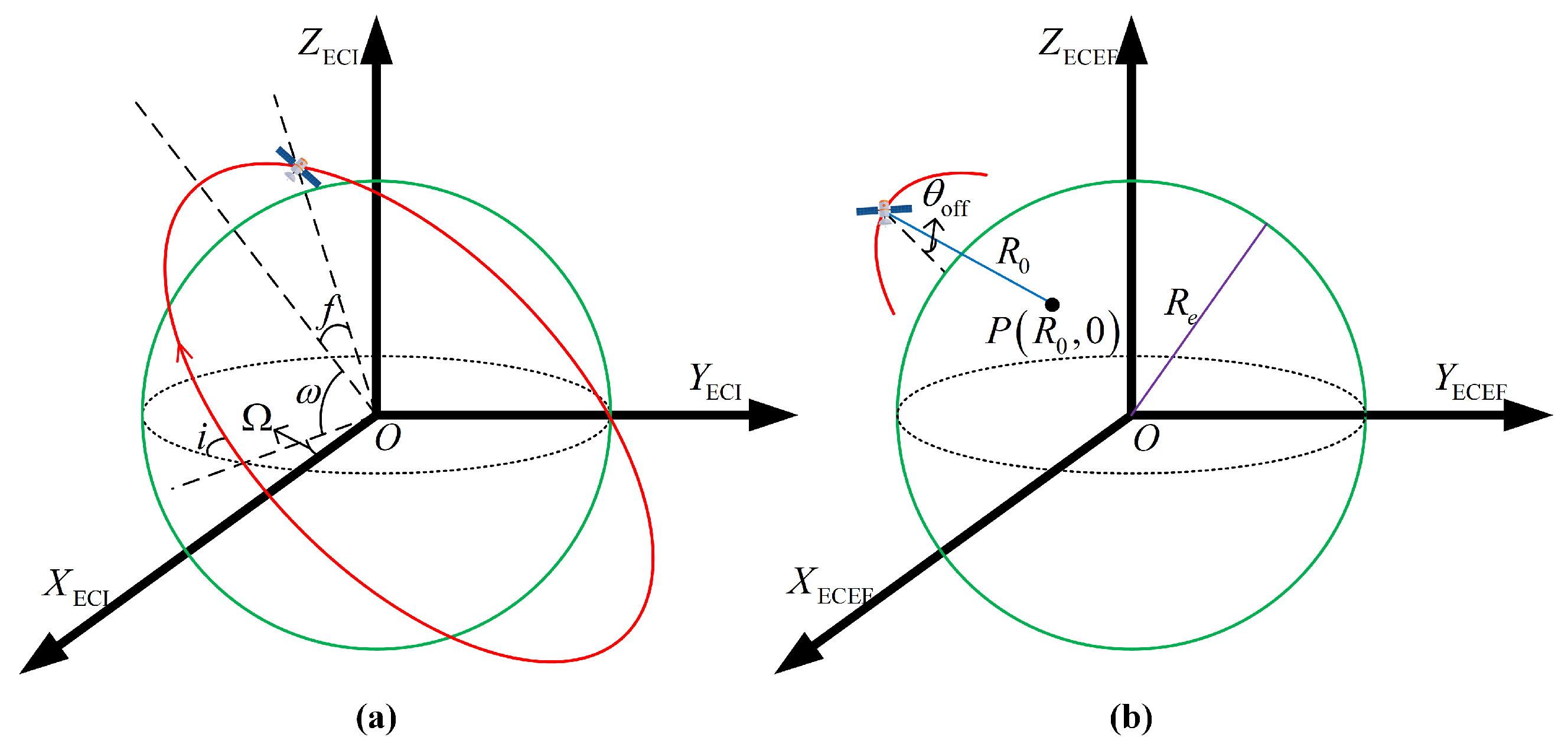
3.1. Curve-Sphere Model

The CUSM treats satellite orbits as general three-dimensional curves while still approximating the Earth as a standard sphere. To facilitate theoretical analysis, we assume the satellite and Earth operate within a two-body model, neglecting orbital deviations caused by perturbations. According to the two-body model in the Earth-Centered Inertial (ECI) coordinate system, the satellite follows a periodic elliptical orbit. Its instantaneous position is determined by six classical orbital elements: semi-major axis a, eccentricity e, orbital inclination i, longitude of the ascending node $\Omega$, argument of periapsis $\omega$, and true anomaly f. Figure 5a illustrates the geometric relationship between the satellite and Earth in the ECI frame, where the green solid line represents the Earth’s surface and the red solid line depicts the satellite’s orbital path.

In the imaging geometry of spaceborne SAR, to maintain the observation scene fixed relative to the satellite, it is necessary to transform the coordinate system to the Earth-Centered, Earth-Fixed (ECEF) frame. Within the ECEF framework, influenced by Earth’s rotation, the satellite trajectory no longer maintains an elliptical form but rather becomes a non-coplanar three-dimensional curve, which significantly complicates the quantitative description of two-dimensional spatial variation characteristics. Figure 5b illustrates the geometric relationship between the satellite and Earth in the ECEF frame. The green solid line represents Earth’s surface, while the red solid line depicts the satellite orbit. At the azimuth central time instant ($t_a=0$), the black dot indicates a target (denoted as $P\left(R_0,0\right)$) located at the intersection of the radar’s zero-Doppler plane and the ground surface with slant range $R_0$. The target’s look angle relative to the satellite is ${\theta }_{\mathrm{off}}$, with the blue solid line representing the target-to-satellite slant range and the purple solid line indicating Earth’s radius $R_e$.

Based on this, we have established the CUSM, where the satellite trajectory is precisely modeled with the Earth assumed to be a perfect sphere. Considering the Earth’s immense size and the operational characteristics of HRWS spaceborne SAR in low Earth orbit (LEO) scenarios, where the side length of the observation area is measured only on the order of hundreds of kilometers, it is theoretically acceptable to approximate the Earth as either a perfect sphere or a local spherical surface during analytical investigations.

In the process of spaceborne SAR imaging, the orbital elements and the radar look angle at the azimuth center time are typically known. Therefore, in CUSM, we can express both the satellite trajectory and target position as functions of known quantities. Consequently, the slant range history can also be represented as a function of these known parameters, thereby establishing a descriptive two-dimensional spatial variation theoretical model.

3.2. Satellite Trajectory

According to Kepler’s equations, the position coordinates of the satellite in ECI are expressed as

$${\mathbf{P}}_{eci}=r_{s}cos\left(f\right)\mathbf{P}+r_{s}sin\left(f\right)\mathbf{Q}$$

(5)

where

$$\begin{array}{cc}\hfill & \mathbf{P}=\left[\begin{array}{c}cos\Omega cos\omega -sin\Omega sin\omega cosi\\ sin\Omega cos\omega +cos\Omega sin\omega cosi\\ sin\omega sini\end{array}\right]\hfill \\ & \mathbf{Q}=\left[\begin{array}{c}-cos\Omega sin\omega -sin\Omega cos\omega cosi\\ -sin\Omega sin\omega +cos\Omega cos\omega cosi\\ cos\omega sini\end{array}\right]\hfill \\ & r_s={\displaystyle \frac{a\left(1-e^2\right)}{1+ecosf}}\hfill \end{array}$$

(6)

The transformation formula for converting a satellite’s position coordinates from ECI to ECEF is expressed as

$$\begin{array}{c}\hfill {\mathbf{P}}_{ecf}=\left[\begin{array}{ccc}cos\varphi & sin\varphi & 0\\ -sin\varphi & cos\varphi & 0\\ 0& 0& 1\end{array}\right]{\mathbf{P}}_{eci}\end{array}$$

(7)

where $\varphi ={\varphi }_0+{\omega }_e{t}_a$, where $t_a$ is the azimuth time, ${\varphi }_0$ represents the rotation angle between ECI and ECEF at the central azimuth time, and $\varphi$ is the rotation angle between ECI and ECEF at time $t_a$. Without loss of generality, we can set $\Omega =0$ and ${\varphi }_0=0$; then, the satellite coordinates in ECEF can be expressed as

$$\begin{array}{cc}\hfill & {\mathbf{P}}_{ecf}={\displaystyle \frac{acosf\left(1-e^2\right)}{1+ecosf}}\left[\begin{array}{c}cos\omega cos\varphi +sin\omega cosisin\varphi \\ -cos\omega sin\varphi +sin\omega cosicos\varphi \\ sin\omega sini\end{array}\right]\hfill \\ & +{\displaystyle \frac{asinf\left(1-e^2\right)}{1+ecosf}}\left[\begin{array}{c}-sin\omega cos\varphi +cos\omega cosisin\varphi \\ sin\omega sin\varphi +cos\omega cosicos\varphi \\ cos\omega sini\end{array}\right]\hfill \end{array}$$

(8)

To further characterize the time variation properties of satellite motion states, we need to express Equation (8) as a function of azimuth time $t_a$. One challenge lies in the absence of an explicit expression for the true anomaly f with respect to $t_a$. However, based on orbital dynamics theory, we can derive an approximate expression of f versus $t_a$ by introducing the satellite’s eccentric anomaly E and mean anomaly M (as shown in Figure 6). To simplify the expression’s complexity, we may assume $f=0$ at the azimuth’s center time. This assumption is justified by two considerations: Firstly, the orbital curvature reaches a maximum at $f=0$, where the azimuth spatial variation becomes most severe. Secondly, the adjustment of the argument of periapsis $\omega$ can regulate the satellite’s geographic position, so setting $f=0$ at azimuth center time does not affect the analysis of the Earth’s rotation effects on the azimuth spatial variation.

Thus, according to the geometric relationship, we have

$$\begin{array}{cc}\hfill & cosf={\displaystyle \frac{cosE-e}{1-ecosE}}\hfill \\ & sinf={\displaystyle \frac{\sqrt{1-e^2}sinE}{1-ecosE}}\hfill \end{array}$$

(9)

Therefore, the multiplicative factor in Equation (8) can be expressed as

$${\displaystyle \frac{acosf\left(1-e^2\right)}{1+ecosf}}={\displaystyle \frac{a\frac{cosE-e}{1-ecosE}\left(1-e^2\right)}{1+e\frac{cosE-e}{1-ecosE}}}=a\left(cosE-e\right)$$

(10)

$${\displaystyle \frac{asinf\left(1-e^2\right)}{1+ecosf}}=a\sqrt{1-e^2}sinE$$

(11)

Thus, we first obtain the expression of f with respect to E. Meanwhile, based on the geometric relationships, it is known that

$$\begin{array}{cc}\hfill & M=E-esinE\hfill \\ \hfill & M=n_s{t}_a\hfill \end{array}$$

(12)

where $n_s=\sqrt{\mu /a^3}$ is the satellite’s mean angular velocity. However, an explicit expression of E in terms of M cannot be obtained directly from Equation (12). Therefore, we first perform a Taylor expansion on M and then employ the series inversion method to derive a polynomial approximation of E in terms of M:

$$\begin{array}{cc}\hfill & M=E-esinE\approx E-e\left(E-E^3/6+E^5/120\right)\hfill \\ \hfill & E\approx {\displaystyle \frac{M}{1-e}}-{\displaystyle \frac{e{M}^3}{6{\left(1-e\right)}^4}}+{\displaystyle \frac{\left(e+9e^2\right)M^5}{120{\left(1-e\right)}^7}}\hfill \end{array}$$

(13)

This approximation yields an error between the E obtained by the series inversion method and the true value smaller than $1\times {10}^{-9}$ within the range $E\in \left[-\pi /8,\pi /8\right]$, as shown in Figure 7a. For typical orbital parameters with semi-major axis $a=6800$ km and eccentricity $e=0.0013$, the resulting errors between Equations (10) and (11) are both less than 0.005 m, as demonstrated in Figure 7b,c.

By substituting Equations (10), (11) and (13) into Equation (8), we obtain the satellite’s ECEF position as a function of the azimuth time $t_a$. For clarity of presentation, we use $x_s$, $y_s$, and $z_s$ to represent the three coordinates of ${\mathbf{P}}_{ecf}$, respectively. Each coordinate is expanded as a Taylor series with respect to $t_a$ (truncated to the fourth order for conciseness), yielding

$$\begin{array}{cc}\hfill & x_s\left(t_a\right)\approx a\left(1-e\right)cos\omega +\left({\displaystyle \frac{a\sqrt{1-e^2}{n}_{s}sin\omega }{e-1}}+a{\omega }_{e}cosisin\omega -ae{\omega }_{e}cosisin\omega \right)t_a\hfill \\ & +\left(-{\displaystyle \frac{a{n}_s^{2}cos\omega }{2{\left(e-1\right)}^2}}-{\displaystyle \frac{a\sqrt{1-e^2}{n}_s{\omega }_{e}cosicos\omega }{e-1}}-{\displaystyle \frac{1}{2}}a{\omega }_e^{2}cos\omega +{\displaystyle \frac{1}{2}}ae{\omega }_e^{2}cos\omega \right)t_a^2\hfill \\ & +\left(\begin{array}{cc}& -{\displaystyle \frac{a{n}_s^2{\omega }_{e}cosisin\omega }{2{(-1+e)}^2}}-{\displaystyle \frac{1}{6}}a{\omega }_e^{3}cosisin\omega +{\displaystyle \frac{1}{6}}ae{\omega }_e^{3}cosisin\omega \hfill \\ & +a\sqrt{1-e^2}\left({\displaystyle \frac{n_s^{3}sin\omega }{6{(e-1)}^4}}-{\displaystyle \frac{n_s{\omega }_e^{2}sin\omega }{2(e-1)}}\right)\hfill \end{array}\right)t_a^3\hfill \\ & +\left(\begin{array}{cc}& -{\displaystyle \frac{a{n}_s^{4}cos\omega }{24{\left(e-1\right)}^5}}-{\displaystyle \frac{ae{n}_s^{4}cos\omega }{8{\left(e-1\right)}^5}}+{\displaystyle \frac{a{n}_s^2{\omega }_e^{2}cos\omega }{4{\left(e-1\right)}^2}}+{\displaystyle \frac{1}{24}}a{\omega }_e^{4}cos\omega \hfill \\ & -{\displaystyle \frac{1}{24}}ae{\omega }_e^{4}cos\omega +a\sqrt{1-e^2}\left(-{\displaystyle \frac{n_s^3{\omega }_{e}cosicos\omega }{6{\left(e-1\right)}^4}}+{\displaystyle \frac{n_s{\omega }_e^{3}cosicos\omega }{6\left(e-1\right)}}\right)\hfill \end{array}\right)t_a^4\hfill \end{array}$$

(14)

$$\begin{array}{cc}\hfill & y_s\left(t_a\right)\approx a\left(1-e\right)cosisin\omega +\left(a\left(e-1\right){\omega }_{e}cos\omega -{\displaystyle \frac{a\sqrt{1-e^2}{n}_{s}cosicos\omega }{e-1}}\right)t_a\hfill \\ & +\left(-{\displaystyle \frac{a\sqrt{1-e^2}{n}_s{\omega }_{e}sin\omega }{e-1}}-{\displaystyle \frac{a{n}_s^{2}cosisin\omega }{2{\left(e-1\right)}^2}}+{\displaystyle \frac{1}{2}}a\left(e-1\right){\omega }_e^{2}cosisin\omega \right)t_a^2\hfill \\ & +\left({\displaystyle \frac{a{n}_s^2{\omega }_{e}cos\omega }{2{\left(e-1\right)}^2}}+{\displaystyle \frac{1}{6}}a\left(1-e\right){\omega }_e^{3}cos\omega +a\sqrt{1-e^2}\left(-{\displaystyle \frac{n_s^{3}cosicos\omega }{6{\left(e-1\right)}^4}}+{\displaystyle \frac{n_s{\omega }_e^{2}cosicos\omega }{2\left(e-1\right)}}\right)\right)t_a^3\hfill \\ & +\left(\begin{array}{cc}& -{\displaystyle \frac{a{n}_s^{4}cosisin\omega }{24{\left(e-1\right)}^5}}-{\displaystyle \frac{ae{n}_s^{4}cosisin\omega }{8{\left(e-1\right)}^5}}+{\displaystyle \frac{a{n}_s^2{\omega }_e^{2}cosisin\omega }{4{\left(e-1\right)}^2}}+\hfill \\ & {\displaystyle \frac{1}{24}}a\left(1-e\right){\omega }_e^{4}cosisin\omega +a\sqrt{1-e^2}\left(-{\displaystyle \frac{n{s}^3{\omega }_{e}sin\omega }{6{\left(e-1\right)}^4}}+{\displaystyle \frac{n_s{\omega }_e^{3}sin\omega }{6\left(e-1\right)}}\right)\hfill \end{array}\right)t_a^4\hfill \end{array}$$

(15)

$$\begin{array}{cc}\hfill & z_s\left(t_a\right)\approx a\left(1-e\right)sinisin\omega +\left({\displaystyle \frac{a\sqrt{1-e^2}}{1-e}}{n}_{s}cos\omega sini\right)t_a-{\displaystyle \frac{a{n}_s^{2}sin\omega sini}{2{\left(e-1\right)}^2}}{t}_a^2\hfill \\ & -{\displaystyle \frac{a\sqrt{1-e^2}{n}_s^{3}cos\omega sini}{6{\left(e-1\right)}^4}}{t}_a^3-{\displaystyle \frac{a\left(1+3e\right)n_s^{4}sin\omega sini}{24{\left(e-1\right)}^5}}{t}_a^4\hfill \end{array}$$

(16)

3.2.1. Slant Range History

After obtaining the expression for the satellite trajectory with respect to the azimuth time $t_a$, we can directly derive the expression for the slant range history based on the geometric relationship:

$$\begin{array}{cc}\hfill & R\left(t_a;R_0,t_p\right)=\sqrt{{\left[x_s\left(t_a\right)-x\left(R_0,t_p\right)\right]}^2+{\left[y_s\left(t_a\right)-y\left(R_0,t_p\right)\right]}^2+{\left[z_s\left(t_a\right)-z\left(R_0,t_p\right)\right]}^2}\hfill \\ & =\sqrt{\begin{array}{cc}& {\left[x_0+x_1{t}_a+x_2{t}_a^2+x_3{t}_a^3+x_4{t}_a^4-x\left(R_0,t_p\right)\right]}^2\hfill \\ & +{\left[y_0+y_1{t}_a+y_2{t}_a^2+y_3{t}_a^3+y_4{t}_a^4-y\left(R_0,t_p\right)\right]}^2\hfill \\ & +{\left[z_0+z_1{t}_a+z_2{t}_a^2+z_3{t}_a^3+z_4{t}_a^4-z\left(R_0,t_p\right)\right]}^2\hfill \end{array}}\hfill \end{array}$$

(17)

Here, $x_m,y_m,z_m\left(m=0,1,2,3,4\right)$ represent the k-th order coefficients of $t_a$ in $x_s,y_s,z_s$, respectively. Meanwhile, ${\left[x\left(R_0,t_p\right),y\left(R_0,t_p\right),z\left(R_0,t_p\right)\right]}^T$ denotes the ECEF position coordinates of targets with slant range $R_0$ along the intersection line between the satellite’s zero-Doppler plane and the Earth’s surface at time $t_p$, which is denoted as ${\mathbf{T}}_{R_0},t_p$.

Expanding Equation (17) with respect to $t_a-t_p$ (for simplicity of presentation, we only expand up to the fourth order) and simplifying, we obtain

$$\begin{array}{cc}\hfill & R\left(t_a;R_0,t_p\right)\approx R_0+{\displaystyle \frac{{\left(t_a-t_p\right)}^2}{2R_0}}\left({\mathbf{V}}_{s,t_p}^2+{\mathbf{A}}_{s,t_p}·\left({\mathbf{P}}_{t_p}-{\mathbf{T}}_{R_0,t_p}\right)\right)\hfill \\ & +{\displaystyle \frac{{\left(t_a-t_p\right)}^3}{R_0}}\left({\displaystyle \frac{1}{2}}{\mathbf{A}}_{s,t_p}·{\mathbf{V}}_{s,t_p}+{\displaystyle \frac{1}{6}}{\dot{\mathbf{A}}}_{s,t_p}·\left({\mathbf{P}}_{t_p}-{\mathbf{T}}_{R_0,t_p}\right)\right)\hfill \\ & +{\displaystyle \frac{{\left(t_a-t_p\right)}^4}{8R_0^3}}\left(\begin{array}{cc}& 4R_c^2\left({\displaystyle \frac{{\mathbf{A}}_{s,t_p}^2}{4}}+{\displaystyle \frac{{\dot{\mathbf{A}}}_{s,t_p}·{\mathbf{V}}_{s,t_p}}{3}}+{\displaystyle \frac{{\ddot{\mathbf{A}}}_{t_p}\left({\mathbf{P}}_{t_p}-{\mathbf{T}}_{R_0,t_p}\right)}{12}}\right)\hfill \\ & -\left({\mathbf{V}}_{s,t_p}^2+{\mathbf{A}}_{s,t_p}·\left({\mathbf{P}}_{t_p}-{\mathbf{T}}_{R_0,t_p}\right)\right)\hfill \end{array}\right)\hfill \end{array}$$

(18)

where ${\mathbf{P}}_{t_p}={\left[x_s\left(t_p\right),y_s\left(t_p\right),z_s\left(t_p\right)\right]}^T$ is the satellite’s ECEF position vector at time $t_p$, while ${\mathbf{V}}_{s,t_p},{\mathbf{A}}_{s,t_p},{\dot{\mathbf{A}}}_{s,t_p},{\ddot{\mathbf{A}}}_{s,t_p}$ represent the first to fourth derivatives of ${\mathbf{P}}_{ecf}$ with respect to $t_a$ evaluated at $t_p$, respectively. Their corresponding x-axis coordinates are

$$\begin{array}{cc}\hfill & x\left(t_p\right)=x_0+x_1{t}_p+x_2{t}_p^2+x_3{t}_p^3+x_4{t}_p^4\hfill \\ & v{x}_s\left(t_p\right)=x_1+2x_2{t}_p+3x_3{t}_p^2+4x_4{t}_p^3\hfill \\ & a{x}_s\left(t_p\right)=2x_2+6x_3{t}_p+12x_4{t}_p^2\hfill \\ & \dot{a}{x}_s\left(t_p\right)=6x_3+24x_4{t}_p\hfill \\ & \ddot{a}{x}_s\left(t_p\right)=24x_4\hfill \end{array}$$

(19)

The same applies to the y-axis coordinate and the z-axis coordinate.

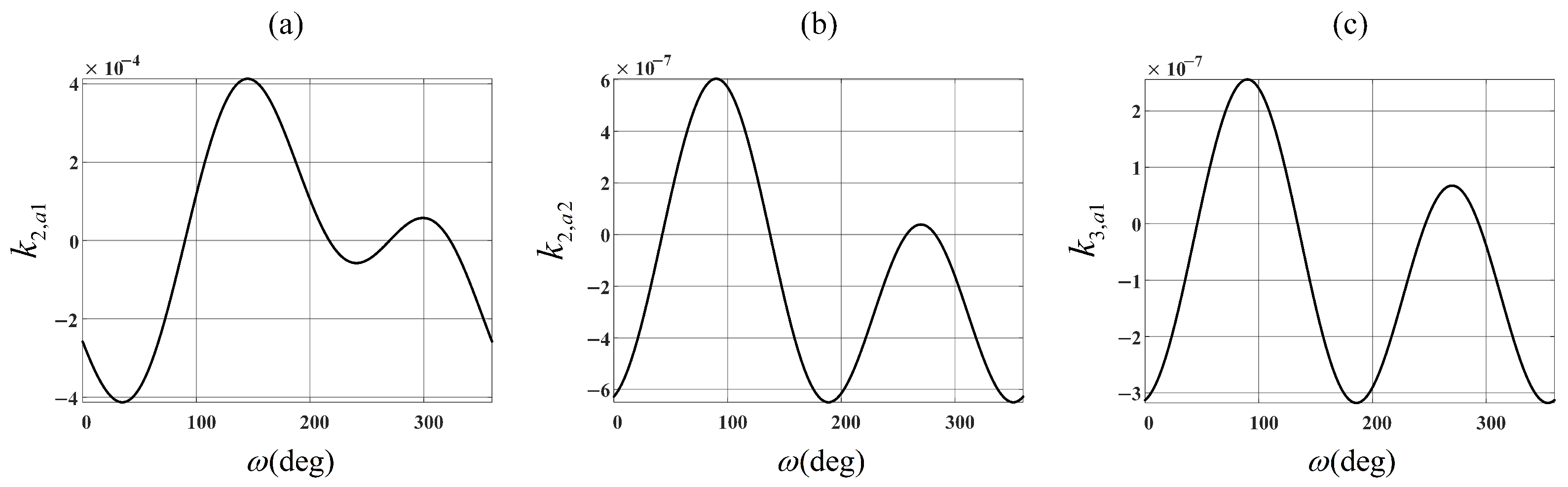
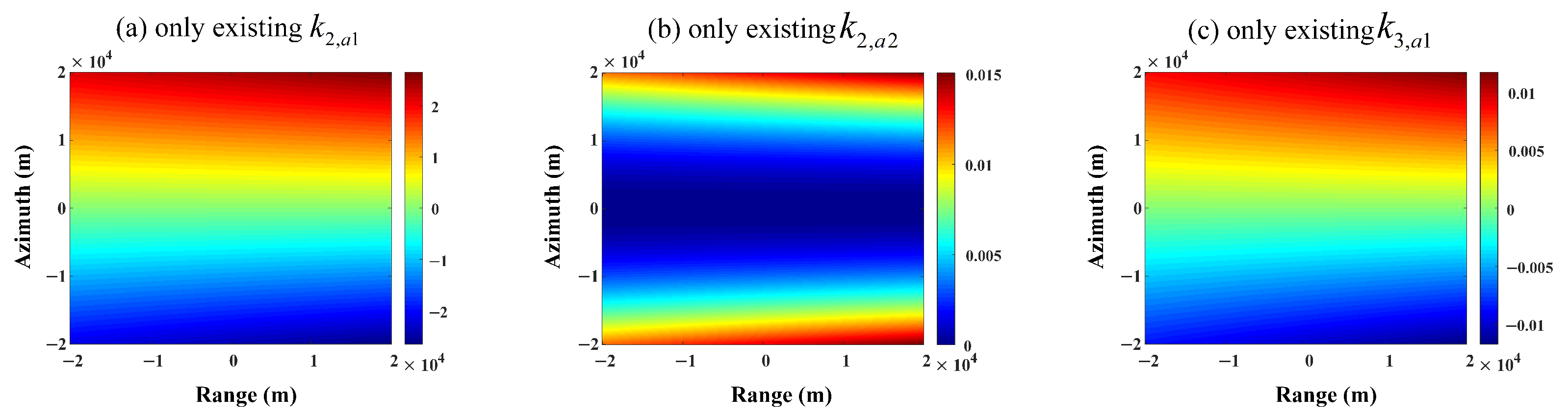
3.2.2. Two-Dimensional Spatial Variation

The coefficients of each order in the term $t_a-t_p$ correspond to $k_n$ in the equation. By expanding $k_n$ in a Taylor series with respect to $t_p$, we can obtain the specific expression of the azimuth’s spatial variation:

$$k_n\approx k_{n,a0}+k_{n,a1}{t}_p+\cdots +k_{n,aj}{t}_p^j$$

(20)

It should be noted that $k_{n,aj}$ is also a function of $R_0$, so the spatial range variation and range-azimuth coupling spatial variation are also included.

According to the empirical findings from Reference [18], it is generally sufficient to consider only the first- and second-order azimuth spatial variation terms of $k_2$ and the first-order azimuth spatial variation term of $k_3$. The remaining azimuth spatial variation terms are sufficiently small to be neglected.

Below, we proceed with the calculations term by term. First, we compute $k_2$. According to the equation,

$$k_2\left(t_p\right)={\displaystyle \frac{{\mathbf{V}}_{s,t_p}^2+{\mathbf{A}}_{s,t_p}·\left({\mathbf{P}}_{t_p}-{\mathbf{T}}_{R_0,t_p}\right)}{2R_0}}$$

(21)

In the equation, the first term in the numerator originates from the spatial variability of the satellite orbit, while the second term arises from the spatial variability of the geometric relationship between the satellite orbit and the ground target. Expanding $k_2$ as a Taylor series with respect to $t_p$,

$$k_2\left(t_p\right)\approx k_{2,a0}+k_{2,a1}{t}_p+k_{2,a2}{t}_p^2$$

(22)

where

$$\begin{array}{cc}\hfill & k_{2,a0}={\displaystyle \frac{{\mathbf{V}}_{s,0}^2+{\mathbf{A}}_{s,0}·\left({\mathbf{P}}_0-{\mathbf{T}}_{R_0,0}\right)}{2R_0}}\hfill \\ & k_{2,a1}={\displaystyle \frac{2{\mathbf{V}}_{s,0}·{\mathbf{A}}_{s,0}+{\dot{\mathbf{A}}}_{s,0}·\left({\mathbf{P}}_0-{\mathbf{T}}_{R_0,0}\right)+{\mathbf{A}}_{s,0}·\left({\mathbf{V}}_{s,0}-{{\mathbf{T}}^{\prime }}_{R_0,0}\right)}{2R_0}}\hfill \\ & k_{2,a2}={\displaystyle \frac{\begin{array}{cc}& 2{\mathbf{A}}_{s,0}·{\mathbf{A}}_{s,0}+2{\mathbf{V}}_{s,0}·{\dot{\mathbf{A}}}_{s,0}+{\ddot{\mathbf{A}}}_{s,0}·\left({\mathbf{P}}_0-{\mathbf{T}}_{R_0,0}\right)\hfill \\ & +2{\dot{\mathbf{A}}}_{s,0}·\left({\mathbf{V}}_{s,0}-{{\mathbf{T}}^{\prime }}_{R_0,0}\right)+{\mathbf{A}}_{s,0}·\left({\mathbf{A}}_{s,0}-{{\mathbf{T}}^{\prime \prime }}_{R_0,0}\right)\hfill \end{array}}{4R_0}}\hfill \end{array}$$

(23)

where ${\mathbf{P}}_0,{\mathbf{V}}_{s,0},{\mathbf{A}}_{s,0},{\dot{\mathbf{A}}}_{s,0},{\ddot{\mathbf{A}}}_{s,0},{\mathbf{T}}_{s,0}$ denote the values of ${\mathbf{P}}_{t_p},{\mathbf{V}}_{s,t_p},{\mathbf{A}}_{s,t_p},{\dot{\mathbf{A}}}_{s,t_p},{\ddot{\mathbf{A}}}_{s,t_p},{\mathbf{T}}_{R_0,t_p}$ at $t_p=0$, while ${{\mathbf{T}}^{\prime }}_{R_0,0},{{\mathbf{T}}^{\prime \prime }}_{R_0,0}$ are the first derivative and second derivative of ${\mathbf{T}}_{R_0,t_p}$ evaluated at $t_p=0$.

In Equation (23), the terms related to the spatial variability of the satellite orbit can be easily expressed using $x_m,y_m,z_m$. However, since it is difficult to obtain precise expressions for the target position coordinates, the terms associated with the spatial variability of the geometric relationship between the satellite orbit and the ground target need to be considered as a whole and appropriately approximated. Specifically, according to orbital motion laws under two-dimensional yaw steering, when f = 0, ${\mathbf{V}}_{s,0}$ is perpendicular to ${\mathbf{P}}_{s,0}$. Therefore, ${\mathbf{P}}_0-{\mathbf{T}}_{R_0,0}$ can be directly derived using geometric relationships:

$${\mathbf{P}}_0-{\mathbf{T}}_{R_0,0}={\displaystyle \frac{{\mathbf{P}}_0}{\left|{\mathbf{P}}_0\right|}}{R}_{0}cos{\theta }_{off}+{\displaystyle \frac{{\mathbf{P}}_0\times {\mathbf{V}}_{s,0}}{\left|{\mathbf{P}}_0\right|\left|{\mathbf{V}}_{s,0}\right|}}{R}_{0}sin{\theta }_{off}$$

(24)

where ${\theta }_{\mathrm{off}}$ represents the azimuth center time and the look angle of the radar. After that, we assume that ${\mathbf{P}}_{t_p}-{\mathbf{T}}_{R_0,t_p}$ always satisfies the above equation (clearly, this inference is not precise, but we only need to obtain the derivatives at $t_p=0$; it has been verified that the error introduced by this approximation is negligible). That is,

$${\mathbf{P}}_{t_p}-{\mathbf{T}}_{R_0,t_p}={\displaystyle \frac{{\mathbf{P}}_{t_p}}{\left|{\mathbf{P}}_0\right|}}{R}_{0}cos{\theta }_{off}+{\displaystyle \frac{{\mathbf{P}}_{t_p}\times {\mathbf{V}}_{s,t_p}}{\left|{\mathbf{P}}_0\right|\left|{\mathbf{V}}_{s,0}\right|}}{R}_{0}sin{\theta }_{off}$$

(25)

By differentiating and then evaluating at $t_p=0$, we obtain

$$\begin{array}{cc}\hfill & {\mathbf{V}}_{s,0}-{{\mathbf{T}}^{\prime }}_{R_0,0}={\displaystyle \frac{{\mathbf{V}}_{s,0}}{\left|{\mathbf{P}}_0\right|}}{R}_{0}cos{\theta }_{off}+{\displaystyle \frac{{\mathbf{P}}_0\times {\mathbf{A}}_{s,0}}{\left|{\mathbf{P}}_0\right|\left|{\mathbf{V}}_{s,0}\right|}}{R}_{0}sin{\theta }_{off}\hfill \\ & {\mathbf{A}}_{s,0}-{{\mathbf{T}}^{\prime \prime }}_{R_0,0}={\displaystyle \frac{{\mathbf{A}}_{s,0}}{\left|{\mathbf{P}}_0\right|}}{R}_{0}cos{\theta }_{off}+{\displaystyle \frac{{\mathbf{V}}_{s,0}\times {\mathbf{A}}_{s,0}+{\mathbf{P}}_0\times {\dot{\mathbf{A}}}_{s,0}}{\left|{\mathbf{P}}_0\right|\left|{\mathbf{V}}_{s,0}\right|}}{R}_{0}sin{\theta }_{off}\hfill \end{array}$$

(26)

In this way, we can represent the spatial-variability-related terms associated with the geometric relationships between the satellite orbit and ground targets using $x_m,y_m,z_m$ as well.

Subsequently, we calculate $k_3$ according to the equation

$$k_3\left(t_p\right)={\displaystyle \frac{1}{R_0}}\left[{\displaystyle \frac{1}{2}}{\mathbf{A}}_{s,t_p}·{\mathbf{V}}_{s,t_p}+{\displaystyle \frac{1}{6}}{\dot{\mathbf{A}}}_{s,t_p}·\left({\mathbf{P}}_{t_p}-{\mathbf{T}}_{R_0,t_p}\right)\right]$$

(27)

Similarly, the first term in the square brackets originates from the spatial variation of the satellite orbit, while the second term arises from the spatial variation in the geometric relationship between the satellite orbit and the ground target. Expanding it with respect to $t_p$, we obtain

$$k_3\left(t_p\right)\approx k_{3,a0}+k_{3,a1}{t}_p$$

(28)

where

$$\begin{array}{cc}\hfill & k_{3,a0}={\displaystyle \frac{1}{R_0}}\left[{\displaystyle \frac{1}{2}}{\mathbf{A}}_{s,0}·{\mathbf{V}}_{s,0}+{\displaystyle \frac{1}{6}}{\dot{\mathbf{A}}}_{s,0}·\left({\mathbf{P}}_0-{\mathbf{T}}_{R_0,0}\right)\right]\hfill \\ & k_{3,a1}={\displaystyle \frac{1}{R_0}}\left[\begin{array}{cc}& {\displaystyle \frac{1}{2}}\left({\dot{\mathbf{A}}}_{s,0}·{\mathbf{V}}_{s,0}+{\mathbf{A}}_{s,0}·{\mathbf{A}}_{s,0}\right)+\hfill \\ & {\displaystyle \frac{1}{6}}\left({\ddot{\mathbf{A}}}_{s,0}·\left({\mathbf{P}}_0-{\mathbf{T}}_{R_0,0}\right)+{\dot{\mathbf{A}}}_{s,0}·\left({\mathbf{V}}_{s,0}-{{\mathbf{T}}^{\prime }}_{R_0,0}\right)\right)\hfill \end{array}\right]\hfill \end{array}$$

(29)

In summary, by utilizing Equations (15)–(19), (25) and (26), we can obtain the expressions of $k_{2,a1}$, $k_{2,a2}$, and $k_{3,a1}$ in terms of known quantities such as orbital elements and look angle, thereby establishing the two-dimensional theoretical spatial variation model. Due to the excessive complexity of the expressions, they are not explicitly provided in this paper. Readers may derive the corresponding expressions using computational tools such as Mathmatica based on the aforementioned equations.

To further demonstrate the relationship between two-dimensional spatial variation and relevant parameters, we conducted a series of Monte Carlo simulations. A set of typical parameters for LEO spaceborne SAR is listed in Table 1. By varying different parameters in the table, we can obtain the variation trends of two-dimensional spatial variation with respect to each parameter.

It should be noted that $R_0$ is not an independent quantity but rather constrained by a, e, and ${\theta }_{\mathrm{off}}$. When $t_a=0$, the following relationship holds:

$$\begin{array}{cc}\hfill & cos{\theta }_{\mathrm{off}}={\displaystyle \frac{R_s^2+R_0^2-R_e^2}{2R_s{R}_0}}\hfill \\ & \Rightarrow R_0=R_{s}cos{\theta }_{\mathrm{off}}-\sqrt{R_e^2-R_s^2{sin}^2{\theta }_{\mathrm{off}}}\hfill \end{array}$$

(30)

where

$$R_s=a\left(1-e\right)$$

(31)

Therefore, when calculating the variation trend of two-dimensional spatial variation, it is necessary to adjust the value of $R_0$ according to $a,e$, and ${\theta }_{\mathrm{off}}$ accordingly. The variation trends of $k_{2,a1}$, $k_{2,a2}$, and $k_{3,a1}$ with respect to i, $\omega$, e, and ${\theta }_{\mathrm{off}}$ are shown in Figure 8, Figure 9, Figure 10, Figure 11 and Figure 12.

From the series of figures above, we can observe several patterns:

(1)

The variation trends of $k_{2,a2}$ and $k_{3,a1}$ are nearly identical, being approximately three orders of magnitude smaller than $k_{2,a1}$.

(2)

The spatial variation appears most severe in polar orbits (with orbital inclination of 90°).

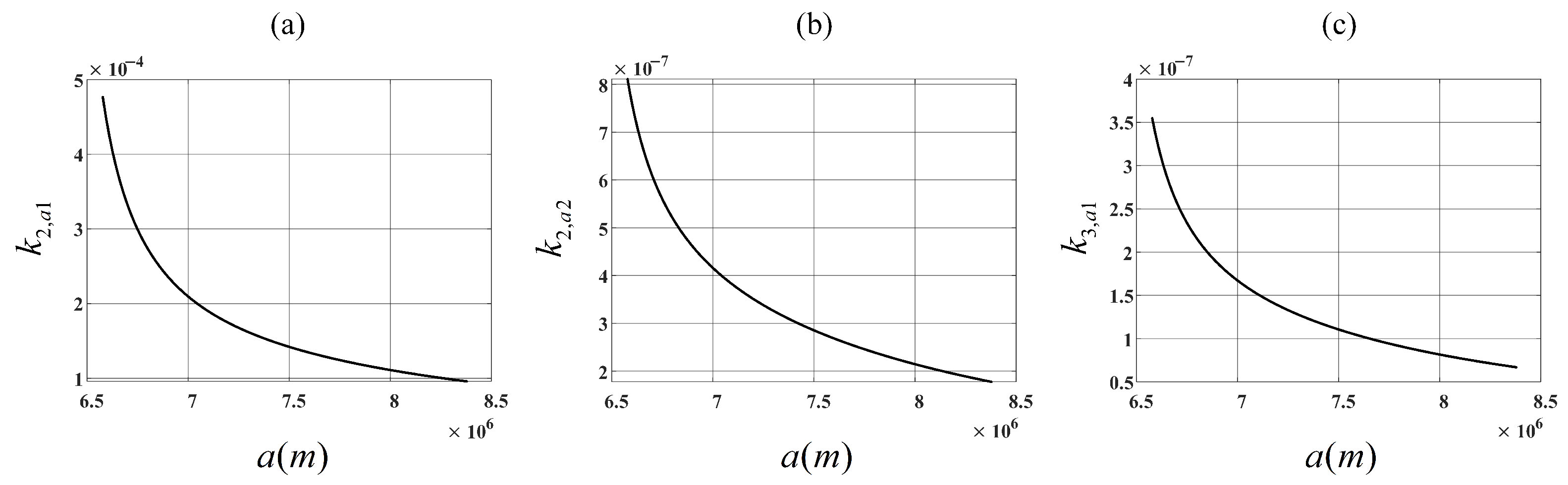
(3)

Spatial variation intensifies with decreasing orbital altitude.

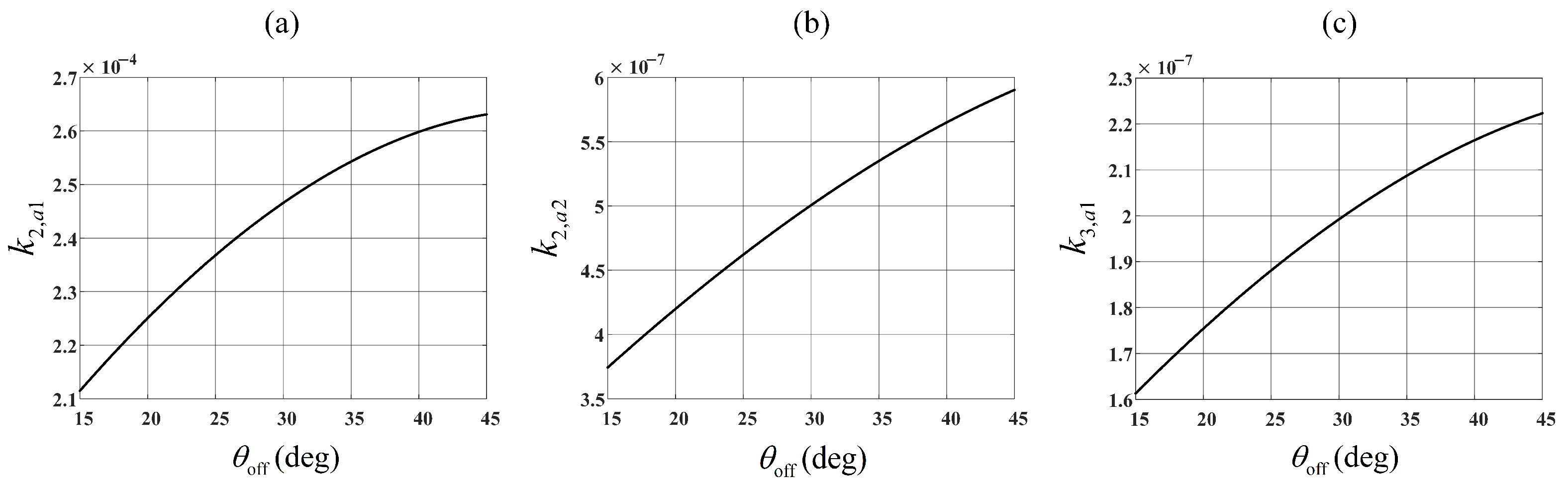
(4)

Larger look angles (which correspond to greater $R_0$ under identical orbital elements) result in more pronounced spatial variation.

However, merely knowing the two-dimensional spatial variation patterns and their magnitude values remains insufficient for subsequent processing. It is further necessary to determine their impacts on imaging based on resolution and observation range parameters, thereby implementing corresponding calibration measures.

4. Analysis of Two-Dimensional Spatial Variation Effects

In the previous section, we established the CUSM to model and describe the satellite trajectory and slant range history, ultimately obtaining the theoretical expression of two-dimensional spatial variation. In this section, we will theoretically analyze the effects of two-dimensional spatial variation. As concluded in [22], the spatial range variation has non-negligible impacts on the quadratic and cubic terms of $f_r$, thus necessitating range blocking. When considering a specific block, the quadratic, cubic, and higher-order terms of $f_r$ with two-dimensional spatial variation can be neglected, requiring only the consideration of the zeroth-order and first-order terms of $f_r$.

4.1. Impact on RCM

The impact of two-dimensional spatial variation on RCM manifests as a first-order phase error in $f_r$. This error phase can be expressed as

$$\Delta {\Phi }_{\mathrm{RCM}}\left(B_r,B_a;R_0,t_p\right)={\varphi }_1\left({\displaystyle \frac{B_a}{2}};R_0,t_p\right){\displaystyle \frac{B_r}{2}}-{\varphi }_1\left({\displaystyle \frac{B_a}{2}};R_{\mathrm{ref}},0\right){\displaystyle \frac{B_r}{2}}$$

(32)

where $R_{\mathrm{ref}}$ represents the shortest slant range to the scene center target, which remains constant when both the orbital elements and look angle are determined. $B_a$ denotes the azimuth bandwidth, and $B_r$ represents the range bandwidth, both determined by the resolution requirements. The ranges of $R_0$ and $t_p$ are defined by the observation scene. Therefore, under identical geometry conditions, higher resolution and larger swath width lead to more pronounced two-dimensional spatial variation effects on RCM. Figure 13 demonstrates the impact of two-dimensional spatial variation on RCM under 0.1 m resolution and 20 km swath width, with satellite–ground geometric parameters listed in Table 1. Subfigures (a), (b), and (c), respectively, show cases where only $k_{2,a1}$, $k_{2,a2}$, and $k_{3,a1}$ components exist. The horizontal coordinate indicates the target’s distribution along the range dimension in the scene, while the vertical coordinate represents the target’s distribution along the azimuth direction. The azimuth distribution of targets in the scene can be approximately obtained by multiplying $t_p$ with the ground velocity of the zero-Doppler plane, i.e.,

$$W_{\mathrm{azim}}\approx V_z{t}_p$$

(33)

where $V_z=\left|{{\mathbf{T}}^{\prime }}_{R_0,0}\right|$. Specifically, according to the equation, the ground-projected velocity of the zero-Doppler surface (it is precisely the ratio of this velocity to the azimuth bandwidth $B_a$ that determines the azimuth resolution) also varies with the orbital elements and the look angle:

$$\begin{array}{cc}\hfill & {{\mathbf{T}}^{\prime }}_{R_0,0}={\mathbf{V}}_{s,0}-\left({\mathbf{V}}_{s,0}-{{\mathbf{T}}^{\prime }}_{R_0,0}\right)\hfill \\ & ={\mathbf{V}}_{s,0}-{\displaystyle \frac{{\mathbf{V}}_{s,0}}{\left|{\mathbf{P}}_0\right|}}{R}_{0}cos{\theta }_{off}-{\displaystyle \frac{{\mathbf{P}}_0\times {\mathbf{A}}_{s,0}}{\left|{\mathbf{P}}_0\right|\left|{\mathbf{V}}_{s,0}\right|}}{R}_{0}sin{\theta }_{off}\hfill \end{array}$$

(34)

From Figure 13, we can observe that among the two-dimensional spatial variation effects, the spatial range variation effect exhibits the most significant variation, which is consistent with the conclusion drawn in literature [22]. According to the analysis in literature [22], severe spatial range variation effects can be corrected using range-blocking methods. Therefore, in this paper, we only need to consider the azimuth spatial variation effects (including range–azimuth coupling spatial variation effects) within a single range block. That is,

$$\Delta {\Phi }_{\mathrm{RCM},\mathrm{av}}\left(B_r,B_a;R_0,t_p\right)={\varphi }_1\left({\displaystyle \frac{B_a}{2}};R_0,t_p\right){\displaystyle \frac{B_r}{2}}-{\varphi }_1\left({\displaystyle \frac{B_a}{2}};R_0,0\right){\displaystyle \frac{B_r}{2}}$$

(35)

Figure 14 demonstrates the impact of azimuth spatial variation effects on RCM under 0.1 m resolution and 20 km swath width conditions, with satellite–ground geometric parameters listed in Table 1. Subfigures (a), (b), and (c), respectively, represent scenarios where only $k_{2,a1}$, $k_{2,a2}$, and $k_{3,a1}$ are present. The results reveal that $\Delta {\Phi }_{\mathrm{RCM},\mathrm{av}}$ consistently remains smaller than $\pi /4$ under these conditions, indicating that two-dimensional spatial variation effects on RCM can be neglected according to the conclusions of [22]. Furthermore, since $\Delta {\Phi }_{\mathrm{RCM},\mathrm{av}}$ becomes negligible when only $k_{2,a2}$ and $k_{3,a1}$ exist, we only need to consider $\Delta {\Phi }_{\mathrm{RCM},\mathrm{av}}$ in the presence of $k_{2,a1}$. By setting $\Delta {\Phi }_{\mathrm{RCM},\mathrm{av}}$ to its upper limit $\pi /4$ and neglecting higher-order terms beyond the cubic order in $f_a$ (which have minimal impact), we derive the HRWS condition requiring the consideration of two-dimensional spatial variation effects on RCM:

$$\left|-\pi {\displaystyle \frac{{\lambda }^2}{c}}{\displaystyle \frac{1}{4k_{2,a0}}}{\displaystyle \frac{B_a^2}{4}}{\displaystyle \frac{B_r}{2}}+\pi {\displaystyle \frac{{\lambda }^2}{c}}{\displaystyle \frac{1}{4\left(k_{2,a0}+k_{2,a1}{t}_p\right)}}{\displaystyle \frac{B_a^2}{4}}{\displaystyle \frac{B_r}{2}}\right|\le {\displaystyle \frac{\pi }{4}}$$

(36)

Utilizing $k_{2,a0}\gg k_{2,a1}{t}_p$, the expression can be simplified to obtain

$$\left|\pi {\displaystyle \frac{{\lambda }^2}{c}}{\displaystyle \frac{B_a^2}{4}}{\displaystyle \frac{B_r}{2}}{\displaystyle \frac{1}{4}}{\displaystyle \frac{k_{2,a1}{t}_p}{k_{2,a0}^2}}\right|\le {\displaystyle \frac{\pi }{4}}$$

(37)

Furthermore, using the formulas for azimuth and range resolution ${\rho }_a=0.886V_z/B_a$ and ${\rho }_r=0.443c/B_r$, Equation (37) can be converted to

$$\left|{\displaystyle \frac{W_{\mathrm{azim}}}{{\rho }_r{\rho }_a^2}}\right|\le {\displaystyle \frac{23k_{2,a0}^2}{{\lambda }^2{k}_{2,a1}{V}_z}}$$

(38)

and this equation is the condition for neglecting the azimuth spatial variation of RCM. When equality holds in the above equation, the corresponding azimuth swath width is defined as the maximum observable swath that allows the azimuth spatial variation of RCM to be neglected:

$$L_{\mathrm{azim},\mathrm{noavRCM}}={\displaystyle \frac{46k_{2,a0}^2{\rho }_r{\rho }_a^2}{{\lambda }^2{k}_{2,a1}{V}_z}}$$

(39)

which can be used as the basis for azimuth blocking.

Under the simulation parameters listed in Figure 1, Figure 15 illustrates the variation of the maximum observable swath with respect to resolution when ignoring the azimuth spatial variation of RCM, where the resolution is varied from 0.01 m to 1 m. Specifically, (a) presents a numerical plot, which more clearly reflects the trend of variation. (b) shows a contour plot, which provides a more intuitive representation of the magnitude of $L_{\mathrm{azim},\mathrm{noavRCM}}$. (c) displays the result of taking the logarithm of the axes in (b), making it easier to observe the values of $L_{\mathrm{azim},\mathrm{noavRCM}}$ at higher resolutions. In more general cases, we often assume ${\rho }_r={\rho }_a$, allowing us to obtain the variation of $L_{\mathrm{azim},\mathrm{noavRCM}}$ with respect to ${\rho }_a$, as shown in Figure 16. Here, (a) demonstrates the variation of $L_{\mathrm{azim},\mathrm{noavRCM}}$ as ${\rho }_a$ varies from 0.01 m to 1 m, with both axes plotted on a logarithmic scale. (b) provides a zoomed-in view of (a), where ${\rho }_a$ varies from 0.1 m to 0.2 m.

4.2. Impact of Azimuth Modulation on Phase Characteristics

Similar to the previous section, the impact of two-dimensional spatial variation on the azimuth modulated phase (AMP) manifests as an error in the zeroth-order term of $f_r$. This phase error is expressed as

$$\Delta {\Phi }_{\mathrm{AMP}}\left(B_r,B_a;R_0,t_p\right)={\varphi }_0\left({\displaystyle \frac{B_a}{2}};R_0,t_p\right)-{\varphi }_0\left({\displaystyle \frac{B_a}{2}};R_{\mathrm{ref}},0\right)$$

(40)

Figure 17 demonstrates the impact of two-dimensional spatial variation on AMP under 0.1 m resolution and 20 km mapping swath conditions, with satellite-ground geometric parameters listed in Table 1. Subfigures (a), (b), and (c), respectively, represent cases where only $k_{2,a1}$, $k_{2,a2}$, and $k_{3,a1}$ exist. Following the conclusions from Reference [22], we can disregard the dominant spatial range variation while focusing solely on the azimuth spatial variation (including range–azimuth coupling spatial variation) within a range block. This can be expressed as

$$\Delta {\Phi }_{\mathrm{AMP},\mathrm{av}}\left(B_r,B_a;R_0,t_p\right)={\varphi }_0\left({\displaystyle \frac{B_a}{2}};R_0,t_p\right)-{\varphi }_0\left({\displaystyle \frac{B_a}{2}};R_0,0\right)$$

(41)

Figure 18 demonstrates the impact of azimuth spatial variation on AMP under 0.1 m resolution and 20 km swath width conditions, with satellite–ground geometric parameters listed in Table 1. Subfigures (a), (b), and (c) correspond to the cases where only $k_{2,a1}$, $k_{2,a2}$, and $k_{3,a1}$ exist, respectively.

Based on the conclusions from [22], $k_{2,a1}$ and $k_{2,a2}$ primarily introduce errors in the quadratic term of $f_a$ in AMP, while $k_{3,a1}$ mainly causes errors in the cubic term of $f_a$. The thresholds for negligible impacts of quadratic and cubic terms of $f_a$ in AMP errors are 0.113$\pi$ and 0.022$\pi$, respectively. Tolerance analyses are subsequently conducted for scenarios involving only $k_{2,a1}$, $k_{2,a2}$, and $k_{3,a1}$ separately. First, assuming only the presence of $k_{2,a1}$ while neglecting higher-order terms of $f_a$ (whose influences are minimal), this condition allows us to disregard the azimuth spatial variation of $\Delta {\Phi }_{\mathrm{AMP},\mathrm{av}}$:

$$\left|\pi {\displaystyle \frac{\lambda }{4}}\left({\displaystyle \frac{1}{k_{2,a0}}}-{\displaystyle \frac{1}{k_{2,a0}+k_{2,a1}{t}_p}}\right){\left({\displaystyle \frac{B_a}{2}}\right)}^2\right|\le 0.113\pi$$

(42)

Using $k_{2,a0}\gg k_{2,a1}{t}_p$, it can be simplified to obtain

$$\left|\pi {\displaystyle \frac{\lambda }{4}}{\displaystyle \frac{k_{2,a1}{t}_p}{k_{2,a0}^2}}{\left({\displaystyle \frac{B_a}{2}}\right)}^2\right|\le 0.113\pi$$

(43)

Furthermore, by using the azimuth resolution formula ${\rho }_a=0.886V_z/B_a$, Equation (43) can be transformed into

$$\left|{\displaystyle \frac{W_{\mathrm{azim}}}{{\rho }_a^2}}\right|\le {\displaystyle \frac{2.3k_{2,a0}^2}{\lambda k_{2,a1}{V}_z}}$$

(44)

and this equation represents the case where the azimuth spatial variation of APM can be neglected when only $k_{2,a1}$ exists. When the equation takes the equals sign, the corresponding azimuth swath width is defined as the maximum swath:

$$L_{\mathrm{azim},\mathrm{noavAPM},\mathrm{k}21}={\displaystyle \frac{4.6k_{2,a0}^2{\rho }_a^2}{\lambda k_{2,a1}{V}_z}}$$

(45)

It can be observed that this width is independent of range resolution, being solely determined by the azimuth resolution under specified spaceborne geometric parameters. Figure 19 illustrates the variation of the maximum swath, neglecting APM errors with azimuth resolution, where both the horizontal and vertical axes are plotted on a logarithmic scale. Here, (a) shows the variation of $L_{\mathrm{azim},\mathrm{noavAPM},\mathrm{k}21}$ as ${\rho }_a$ varies from 0.01 m to 1 m. (b) provides a zoomed-in view of (a), where ${\rho }_a$ varies from 0.1 m to 0.2 m.

Secondly, assume only the existence of $k_{2,a2}$, neglecting quadratic and higher terms in $f_a$ (which have a minimal impact). Under this condition, it becomes unnecessary to consider the azimuth spatial variation of $\Delta {\Phi }_{\mathrm{AMP},\mathrm{av}}$:

$$\left|\pi {\displaystyle \frac{\lambda }{4}}\left({\displaystyle \frac{1}{k_{2,a0}}}-{\displaystyle \frac{1}{k_{2,a0}+k_{2,a2}{t}_p^2}}\right){\left({\displaystyle \frac{B_a}{2}}\right)}^2\right|\le 0.113\pi$$

(46)

Using the condition $k_{2,a0}\gg k_{2,a2}{t}_p^2$, we can simplify to obtain

$$\begin{array}{cc}\hfill & \left|\pi {\displaystyle \frac{\lambda }{4}}{\displaystyle \frac{k_{2,a2}{t}_p^2}{k_{2,a0}^2}}{\left({\displaystyle \frac{B_a}{2}}\right)}^2\right|\le 0.113\pi \hfill \\ & \Rightarrow {\displaystyle \frac{W_{\mathrm{azim}}^2}{{\rho }_a^2}}\le {\displaystyle \frac{2.3k_{2,a0}^2}{\lambda \left|k_{2,a2}\right|}}\hfill \end{array}$$

(47)

When the equality holds in the above equation, we define the azimuth swath width at this time as the maximum swath:

$$L_{\mathrm{azim},\mathrm{noavAPM},\mathrm{k}22}=2{\rho }_a\sqrt{{\displaystyle \frac{2.3k_{2,a0}^2}{\lambda \left|k_{2,a2}\right|}}}$$

(48)

Finally, assume that only $k_{3,a1}$ exists while neglecting the third-order and higher terms of $f_a$ (whose effects are negligible). Under this condition, it is unnecessary to consider the azimuth spatial variation of $\Delta {\Phi }_{\mathrm{AMP},\mathrm{av}}$:

$$\left|\pi {\displaystyle \frac{{\lambda }^2}{16}}\left({\displaystyle \frac{k_{3,a0}+k_{3,a1}{t}_p}{k_{2,a0}^3}}-{\displaystyle \frac{k_{3,a0}}{k_{2,a0}^3}}\right){\left({\displaystyle \frac{B_a}{2}}\right)}^3\right|\le 0.022\pi$$

(49)

The expression can be further simplified to obtain

$$\left|{\displaystyle \frac{W_{\mathrm{azim}}}{{\rho }_a^3}}\right|\le {\displaystyle \frac{4.05k_{2,a0}^3}{{\lambda }^2{k}_{3,a1}{V}_z^2}}$$

(50)

When the equality holds in the above equation, the azimuth swath width at this point is defined as the maximum swath:

$$L_{\mathrm{azim},\mathrm{noavAPM},\mathrm{k}31}={\displaystyle \frac{8.1k_{2,a0}^3{\rho }_a^3}{{\lambda }^2{k}_{3,a1}{V}_z^2}}$$

(51)

Figure 20 illustrates the variation of the maximum swath, ignoring APM error with azimuth resolution, where both axes are plotted on a logarithmic scale. Here, (a) shows the case when ${\rho }_a$ varies from 0.01 m to 1 m. (b) provides a zoomed-in view of (a), where ${\rho }_a$ varies from 0.1 m to 0.2 m.

Figure 21 illustrates the variation of maximum swath with azimuth resolution when APM errors are ignored, where both axes employ logarithmic scales. Here, (a) demonstrates the variation of $L_{\mathrm{azim},\mathrm{noavAPM},\mathrm{k}31}$ when ${\rho }_a$ varies from 0.01 m to 1 m. (b) provides a zoomed-in view of (a), where ${\rho }_a$ varies from 0.1 m to 0.2 m.

In summary, the impact of two-dimensional spatial variation (primarily azimuth spatial variation) on imaging is related to both the satellite–ground geometric relationship and parameters such as resolution and azimuth swath. To further demonstrate the relationship between spatial variation effects and various parameters, Figure 22, Figure 23, Figure 24, Figure 25, Figure 26 and Figure 27 shows the variations of Equations (39), (45), (48) and (51) with different parameters. For visualization purposes, the portions of $L_{\mathrm{azim},\mathrm{noavAPM},\mathrm{k}21}$ exceeding 100 km are set to 100 km, while other maximum azimuth swaths exceeding 1000 km are set to 1000 km.

5. Two-Dimensional Spatial Variation Processing Methods

From the analysis in Section 4, we can observe that $L_{\mathrm{azim},\mathrm{noavRCM}}$, $L_{\mathrm{azim},\mathrm{noavAPM},\mathrm{k}22}$, and $L_{\mathrm{azim},\mathrm{noavAPM},\mathrm{k}31}$ are relatively large, while $L_{\mathrm{azim},\mathrm{noavAPM},\mathrm{k}21}$ is significantly smaller. In HRWS spaceborne SAR, constrained by the enormous data volume, we typically maintain the ratio of the azimuth swath to the azimuth resolution within ${10}^5$. This implies that, in most cases, we do not need to consider the azimuth spatial variation of ${\varphi }_1$. Only the azimuth spatial variation of ${\varphi }_0$ with respect to $k_{2,a1}$ needs to be taken into account. However, in extreme cases (e.g., when the resolution is very high), considering only the azimuth spatial variation of ${\varphi }_0$ with respect to $k_{2,a1}$ may be insufficient, and azimuth blocking would then be required.

With the aforementioned analysis, we propose a two-dimensional spatial variation correction algorithm based on azimuth nonlinear chirp scaling (ANCS) processing. This algorithm is developed from the spatial range variation correction algorithm using the range-blocking method presented in [22]. The flowchart of the proposed algorithm is illustrated in Figure 28. The complete algorithm consists of two main components, marked by red and green dashed boxes: preprocessing and range blocking, respectively. The range blocking further comprises three sub-modules, indicated by yellow, purple and blue dashed boxes: spatial range variation correction, azimuth NCS processing, and azimuth compression.

The preprocessing stage aims to eliminate spectral aliasing introduced by azimuth beam scanning and perform unified phase processing using the parameters of reference targets. The spatial range variation correction stage removes spatial range variation components, including RCM and the higher-order terms of $f_r$ through processing on each block. The azimuth compression stage eliminates spatial range variation components of the azimuth modulation phase while completing azimuth compression for each range cell. Detailed derivations and formula representations for these stages have been comprehensively presented in [22] and will not be reiterated here. The key distinction between our algorithm and [22] lies in the execution sequence of azimuth compression: our method performs azimuth compression within each range block, whereas the referenced algorithm implements azimuth compression after merging range blocks. However, since both approaches require operations on each range cell for azimuth compression, there is no essential difference in their final implementation.

The following section primarily introduces the newly added azimuth NCS processing component.

5.1. Azimuth Nonlinear Chirp Scaling Processing

In most cases, we can consider only the first-order azimuth spatial variation of $k_2$ while ignoring the azimuth spatial variations of other coefficients. Moreover, we only need to consider the influence of $k_2$’s first-order azimuth spatial variation on ${\varphi }_0$. However, according to previous analysis, the first-order azimuth spatial variation coefficient $k_{2,a1}$ of $k_2$ varies with range, so its correction needs to be implemented during the range blocking. After completing the range block compensation for the first-order and higher terms of $f_r$, the range-Doppler domain signal of $P\left(R_0,t_p\right)$ can be expressed as

$$\begin{array}{cc}\hfill & s{S}_{\mathrm{after}\_\mathrm{block}}\left(t_r,f_a;R_0,t_p\right)=\mathrm{sinc}(t_r-{\displaystyle \frac{2R_0}{c}})\hfill \\ & \times exp\left(-j4\pi {\displaystyle \frac{R_0}{\lambda }}\right)exp\left(-j2\pi t_p{f}_a\right)\hfill \\ & \times exp\left(j{\varphi }_0\left(f_a;R_0,t_p\right)\right)exp\left(j\pi {\displaystyle \frac{f_a^2}{K_c}}\right)\hfill \end{array}$$

(52)

where $K_c$ represents the chirp rate introduced by the azimuth time–frequency transformation. The presence of this term causes aliasing in the azimuth time domain. Therefore, we first perform an inverse azimuth time-frequency transform to restore the original chirp characteristics of the signal. After that, the target signal is transformed into the two-dimensional time domain as

$$\begin{array}{cc}\hfill & s{s}_{\mathrm{after}\_\mathrm{block}}\left(t_r,t_a;R_0,t_p\right)=\mathrm{sinc}(t_r-{\displaystyle \frac{2R_0}{c}})\hfill \\ & \times exp\left\{-j{\displaystyle \frac{4\pi }{\lambda }}\left[\begin{array}{cc}& R_0+k_2{\left(t_a-t_p\right)}^2+k_3{\left(t_a-t_p\right)}^3\hfill \\ & +k_4{\left(t_a-t_p\right)}^4+k_5{\left(t_a-t_p\right)}^5+k_6{\left(t_a-t_p\right)}^6\hfill \end{array}\right]\right\}\hfill \end{array}$$

(53)

If we compensate the above equation with a cubic time phase,

$$H_{\mathrm{av},\mathrm{time}}=exp\left(-j{\displaystyle \frac{4\pi }{\lambda }}{p}_3{t}_a^3\right)$$

(54)

Multiplying Equation (53) by Equation (54) and expanding $k_2$ as $k_{2,a0}+k_{2,a1}{t}_p$, we obtain

$$\begin{array}{cc}\hfill & s{s}_{\mathrm{after}\_\mathrm{av}\_\mathrm{time}}\left(t_r,t_a;R_0,t_p\right)=\mathrm{sinc}(t_r-{\displaystyle \frac{2R_0}{c}})\hfill \\ & \times exp\left\{-j{\displaystyle \frac{4\pi }{\lambda }}\left[\begin{array}{cc}& R_0+p_3{t}_p^3+3p_3{t}_p^2\left(t_a-t_p\right)+\left(k_{2,a0}+k_{2,a1}{t}_p+3p_3{t}_p\right){\left(t_a-t_p\right)}^2\hfill \\ & +\left(k_3+p_3\right){\left(t_a-t_p\right)}^3+k_4{\left(t_a-t_p\right)}^4+k_5{\left(t_a-t_p\right)}^5+k_6{\left(t_a-t_p\right)}^6\hfill \end{array}\right]\right\}\hfill \end{array}$$

(55)

It can be observed that by setting $p_3=-k_{2,a1}/3$, the azimuth spatial variation of $k_2$ can be eliminated. Moreover, since the absolute value of $k_{2,a1}$ is very small, the impact of the zeroth-order and first-order terms of $t_a-t_p$ introduced by this can be neglected. It should be noted that here, $k_{2,a1}$ is obtained by the polynomial fitting of $k_2$ to avoid the influence of insufficient precision in the theoretical model, and the fitting method has been provided in [22]. Thus, Equation (54) can be rewritten as

$$H_{\mathrm{av},\mathrm{time}}=exp\left(j{\displaystyle \frac{4\pi }{\lambda }}{\displaystyle \frac{k_{2,a1}}{3}}{t}_a^3\right)$$

(56)

Equation (55) can be rewritten as

$$\begin{array}{cc}\hfill & s{s}_{\mathrm{after}\_\mathrm{av}\_\mathrm{time}}\left(t_r,t_a;R_0,t_p\right)=\mathrm{sinc}(t_r-{\displaystyle \frac{2R_0}{c}})\hfill \\ & \times exp\left\{-j{\displaystyle \frac{4\pi }{\lambda }}\left[\begin{array}{cc}& R_0+k_{2,a0}{\left(t_a-t_p\right)}^2+\left(k_3+p_3\right){\left(t_a-t_p\right)}^3\hfill \\ & +k_4{\left(t_a-t_p\right)}^4+k_5{\left(t_a-t_p\right)}^5+k_6{\left(t_a-t_p\right)}^6\hfill \end{array}\right]\right\}\hfill \end{array}$$

(57)

After performing the azimuth time–frequency transformation again, Equation (57) is transformed into the Range-Doppler (RD) domain, yielding

$$\begin{array}{cc}\hfill & s{s}_{\mathrm{after}\_\mathrm{av}\_\mathrm{time}}\left(t_r,t_a;R_0,t_p\right)=\mathrm{sinc}(t_r-{\displaystyle \frac{2R_0}{c}})exp\left(-j4\pi {\displaystyle \frac{R_0}{\lambda }}\right)exp\left(-j2\pi t_p{f}_a\right)exp\left(j\pi {\displaystyle \frac{f_a^2}{K_c}}\right)\hfill \\ & \times exp\left[j\left(\begin{array}{cc}& \pi {\displaystyle \frac{\lambda }{4}}{\displaystyle \frac{1}{k_{2,a0}}}{f}_a^2+\pi {\displaystyle \frac{{\lambda }^2}{16}}{\displaystyle \frac{k_{3,new}}{k_{2,a0}^3}}{f}_a^3+\pi {\displaystyle \frac{{\lambda }^3}{256}}{\displaystyle \frac{9k_{3,new}^2-4k_{2,a0}{k}_4}{k_{2,a0}^5}}{f}_a^4\hfill \\ & +\pi {\displaystyle \frac{{\lambda }^4}{1024}}{\displaystyle \frac{27k_{3,new}^3-24k_{2,a0}{k}_{3,new}{k}_4+4k_{2,a0}^2{k}_5}{k_{2,a0}^7}}{f}_a^5\hfill \\ & +\pi {\displaystyle \frac{{\lambda }^5}{8192}}{\displaystyle \frac{189k_{3,new}^4-252k_{2,a0}{k}_{3,new}^2{k}_4+32k_{2,a0}^2{k}_4^2+60k_{2,a0}^2{k}_{3,new}{k}_5-8k_{2,a0}^3{k}_6}{k_{2,a0}^9}}{f}_a^6\hfill \end{array}\right)\right]\hfill \end{array}$$

(58)

where $k_{3,new}=k_3+p_3$. After this, there is no longer any azimuth spatial variation in the last phase term of the aforementioned equation, and the azimuth pulse compression can be performed for each range cell using $H_{\mathrm{ac}}$ from [22].

5.2. Algorithm Extensions

In the algorithm shown in Figure 28, only the influence of $k_{2,a1}$ on the azimuth modulation phase (${\varphi }_0$) is considered, which is applicable to the vast majority of cases. However, according to the analysis in Section 4, when the resolution becomes extremely high, the effects of rest azimuth spatial variation need to be taken into account. Therefore, when necessary, the algorithm requires extension. This extension corresponds to azimuth blocking.

Azimuth blocking is mainly divided into two scenarios. The first scenario involves considering the impact of $k_{2,a1}$ on RCM, i.e., $L_{\mathrm{azim},\mathrm{real}}<L_{\mathrm{azim},\mathrm{noavRCM}}$, where $L_{\mathrm{azim},\mathrm{real}}$ represents the actual azimuth swath in a single imaging process. In this case, azimuth blocking should be performed according to $L_{\mathrm{azim},\mathrm{noavRCM}}$ after spatial range variation correction and before ANCS processing. Since the $k_n$ corresponding to different $R_0$ and $t_p$ can be precisely calculated by polynomial fitting coefficient, or each azimuth block, $k_n$ can be corrected based on the $t_{p,\mathrm{ablock}}$ of its central target. The specific compensation factor can be expressed as

$$\begin{array}{cc}\hfill & H_{\mathrm{ablock}}\left(f_r,f_a;R_{\mathrm{block}},t_{p,\mathrm{ablock}}\right)=\mathrm{conj}\left\{\begin{array}{cc}& S{S}_{\mathrm{receive}}\left(f_r,f_a;R_{\mathrm{block}},t_{p,\mathrm{ablock}}\right)\hfill \\ & \times exp\left[-j{\varphi }_0\left(f_a;R_{\mathrm{block}},t_{p,\mathrm{ablock}}\right)\right]exp\left(j4\pi {\displaystyle \frac{f_c+f_r}{c}}{R}_{\mathrm{block}}\right)\hfill \end{array}\right\}\hfill \\ & \times \left\{\begin{array}{cc}& S{S}_{\mathrm{receive}}\left(f_r,f_a;R_{\mathrm{block}},0\right)\hfill \\ & \times exp\left[-j{\varphi }_0\left(f_a;R_{\mathrm{block}},0\right)\right]exp\left(j4\pi {\displaystyle \frac{f_c+f_r}{c}}{R}_{\mathrm{block}}\right)\hfill \end{array}\right\}\hfill \end{array}$$

(59)

The second scenario requires the consideration of the influence of $k_{2,a2}$ and $k_{3,a1}$ on the azimuth modulation phase, i.e., when $L_{\mathrm{azim},\mathrm{real}}<L_{\mathrm{azim},\mathrm{noavAPM},\mathrm{k}22}$ or $L_{\mathrm{azim},\mathrm{real}}<L_{\mathrm{azim},\mathrm{noavAPM},\mathrm{k}31}$. These two cases can be discussed collectively by performing azimuth blocking after completing ANCS and before azimuth compression, using $\mathit{min}\left\{L_{\mathrm{azim},\mathrm{noavAPM},\mathrm{k}22}\right\},$$\left\{L_{\mathrm{azim},\mathrm{noavAPM},\mathrm{k}31}\right\}$ as the blocking criterion. For each azimuth block, the corresponding azimuth compression function can then be selected according to its respective $t_{p,\mathrm{ablock}}$:

$$H_{\mathrm{ac},\mathrm{block}}\left(f_a;R_0,t_{p,\mathrm{ablock}}\right)=exp\left(-j{\varphi }_0\left(f_a;R_0,t_{p,\mathrm{ablock}}\right)\right)exp\left(-j\pi {\displaystyle \frac{f_a^2}{K_c}}\right)$$

(60)

To verify the necessity and effectiveness of this azimuth blocking method, we conducted a series of simulation experiments. The simulation parameters are shown in Table 1. Notably, to reduce $L_{\mathrm{azim},\mathrm{noavAPM},\mathrm{k}22}$ and $L_{\mathrm{azim},\mathrm{noavAPM},\mathrm{k}31}$, we set the wavelength to 0.06 m. In the simulation, the azimuth resolution is set to 0.1 m, and the width of the observation scene in the azimuth direction is set to 200 km. Five targets are configured in the simulation, all having the same closest slant range, with azimuth positions at −100 km, −50 km, 0 km, 50 km, and 100 km. The azimuth block length is sequentially set from 1 km to 100 km, and the imaging quality assessment results for the five targets are shown in Figure 29.

According to the calculations from Equations (48) and (51), $L_{\mathrm{azim},\mathrm{noavAPM},\mathrm{k}22}$ is 78.45 km, and $L_{\mathrm{azim},\mathrm{noavAPM},\mathrm{k}31}$ is 19.87 km, with $L_{\mathrm{azim},\mathrm{noavAPM},\mathrm{k}31}$ being the smaller one. Therefore, the results in the figure indicate that when the azimuth block length is less than $L_{\mathrm{azim},\mathrm{noavAPM},\mathrm{k}31}$, the imaging quality for all targets meets our required criteria (PSLR > 13 dB). Thus, when necessary, azimuth blocking is required, and the azimuth block length should be appropriately selected.

6. Experiments and Results

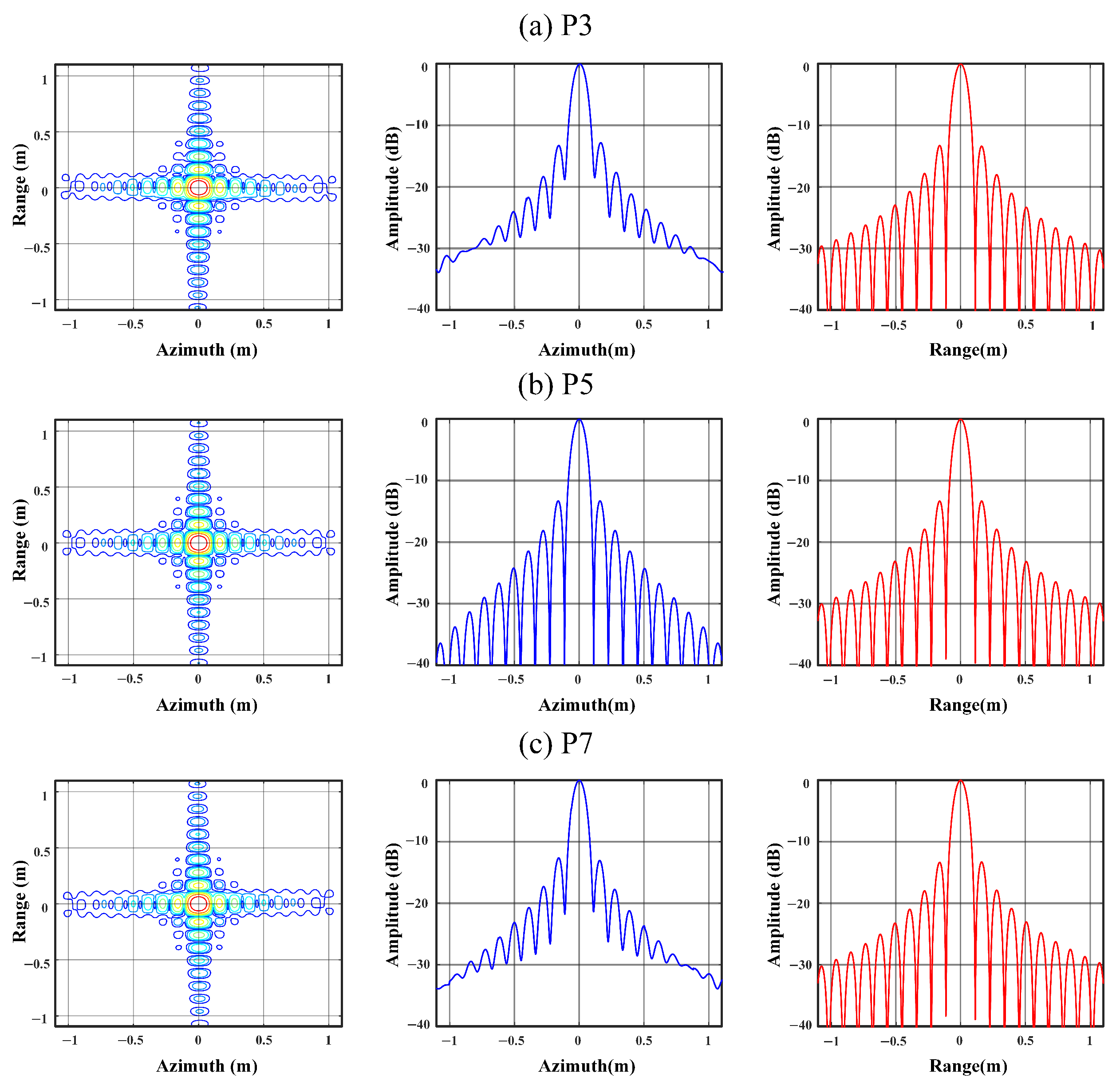
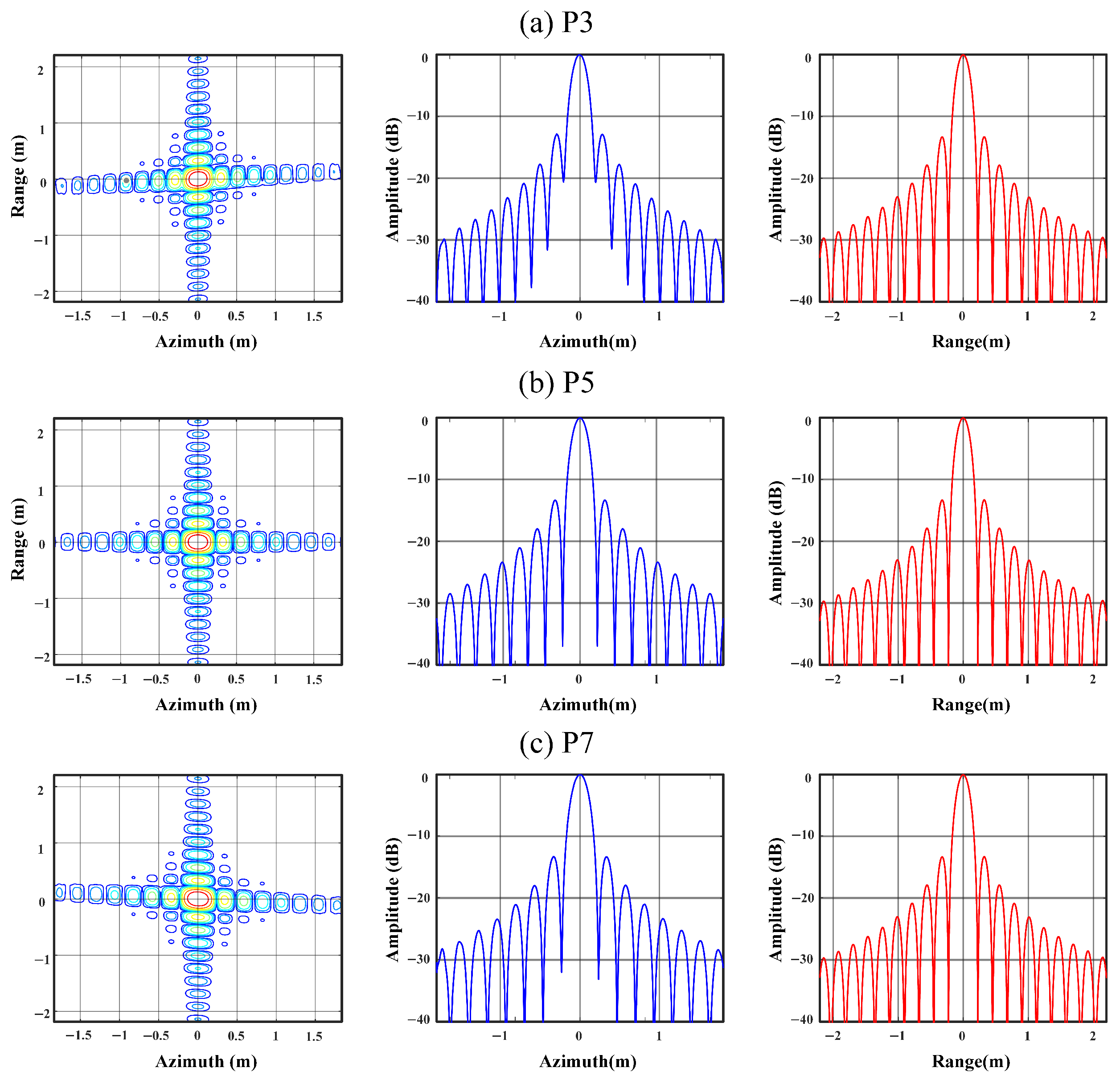
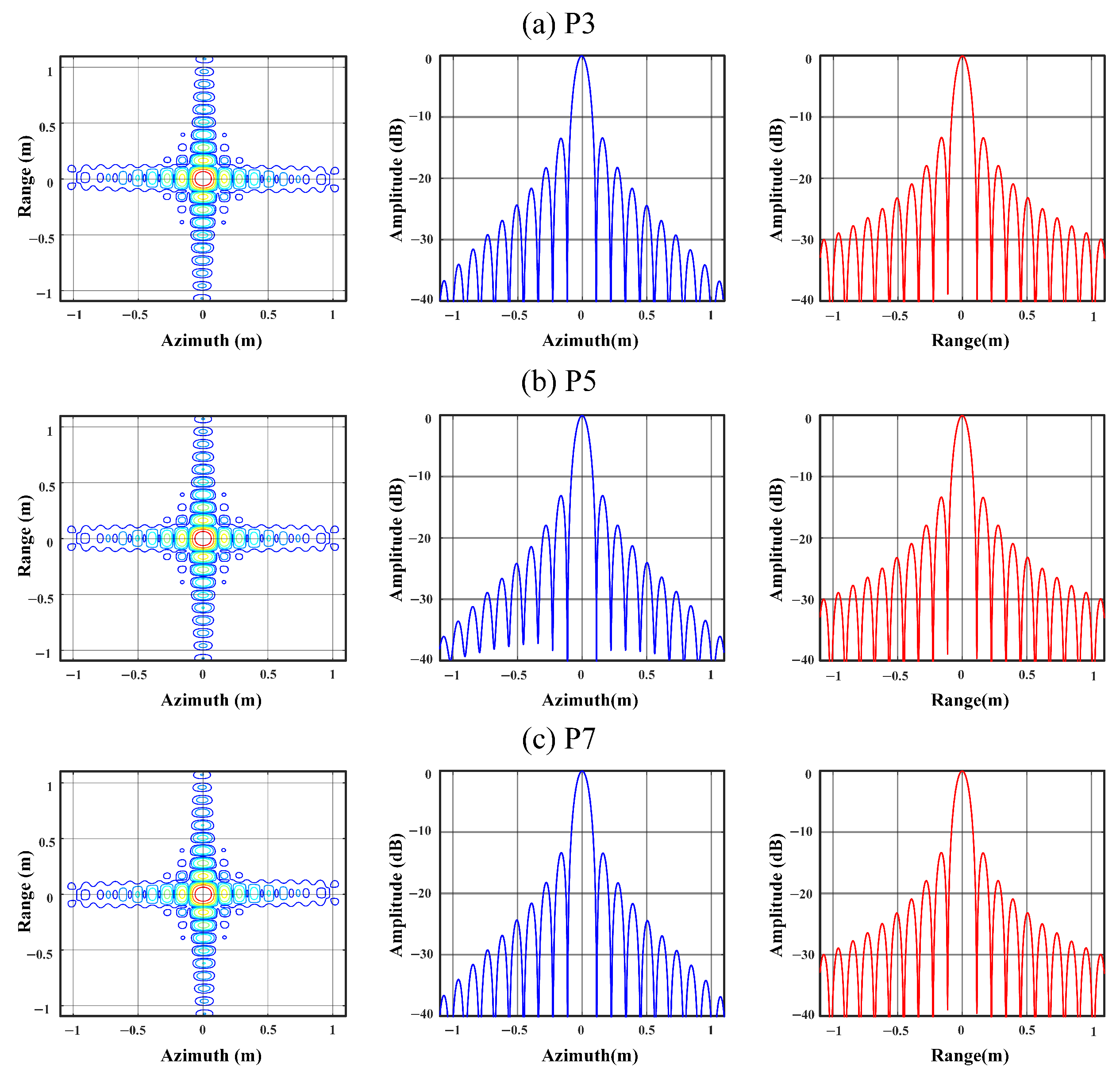
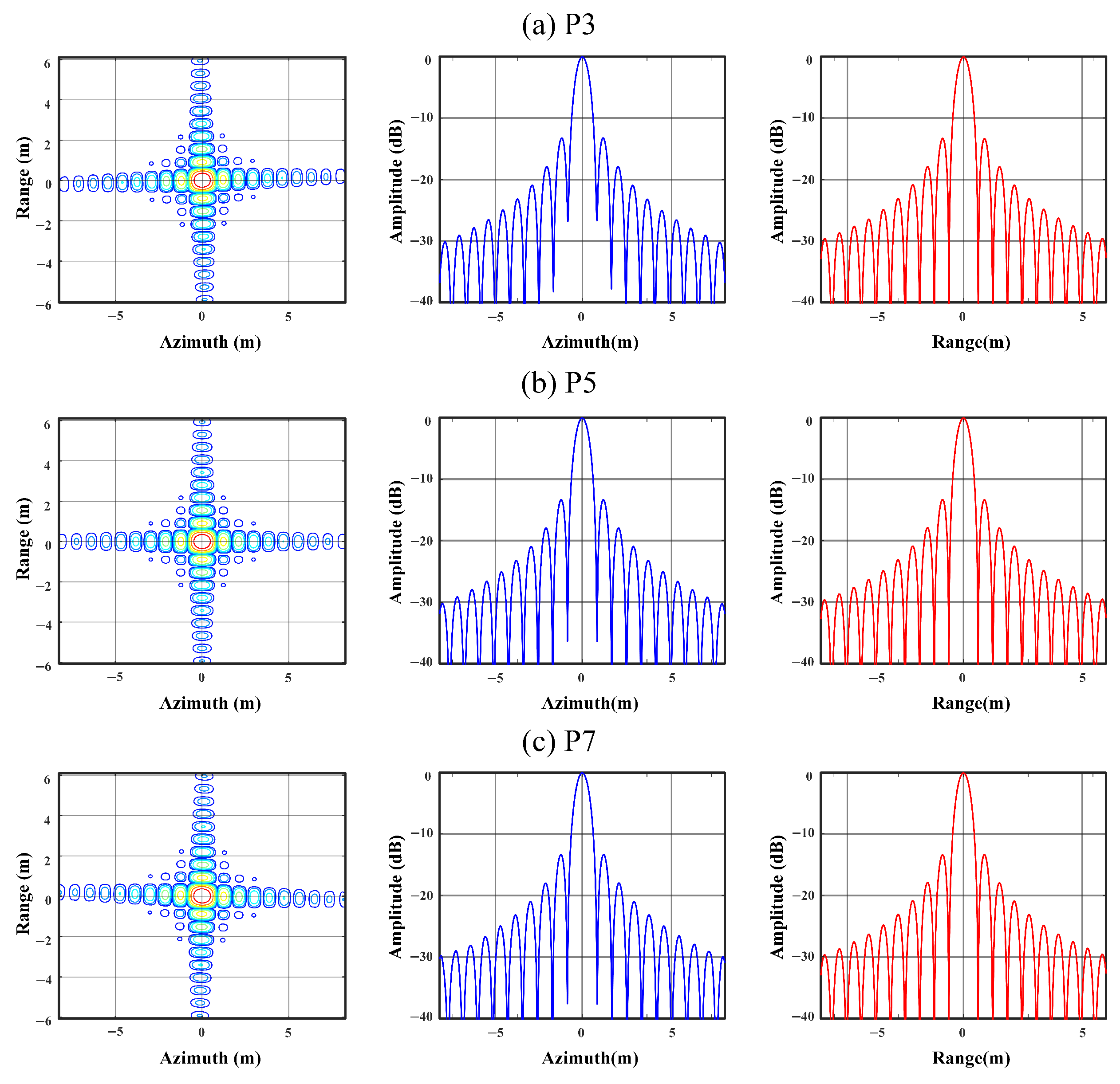
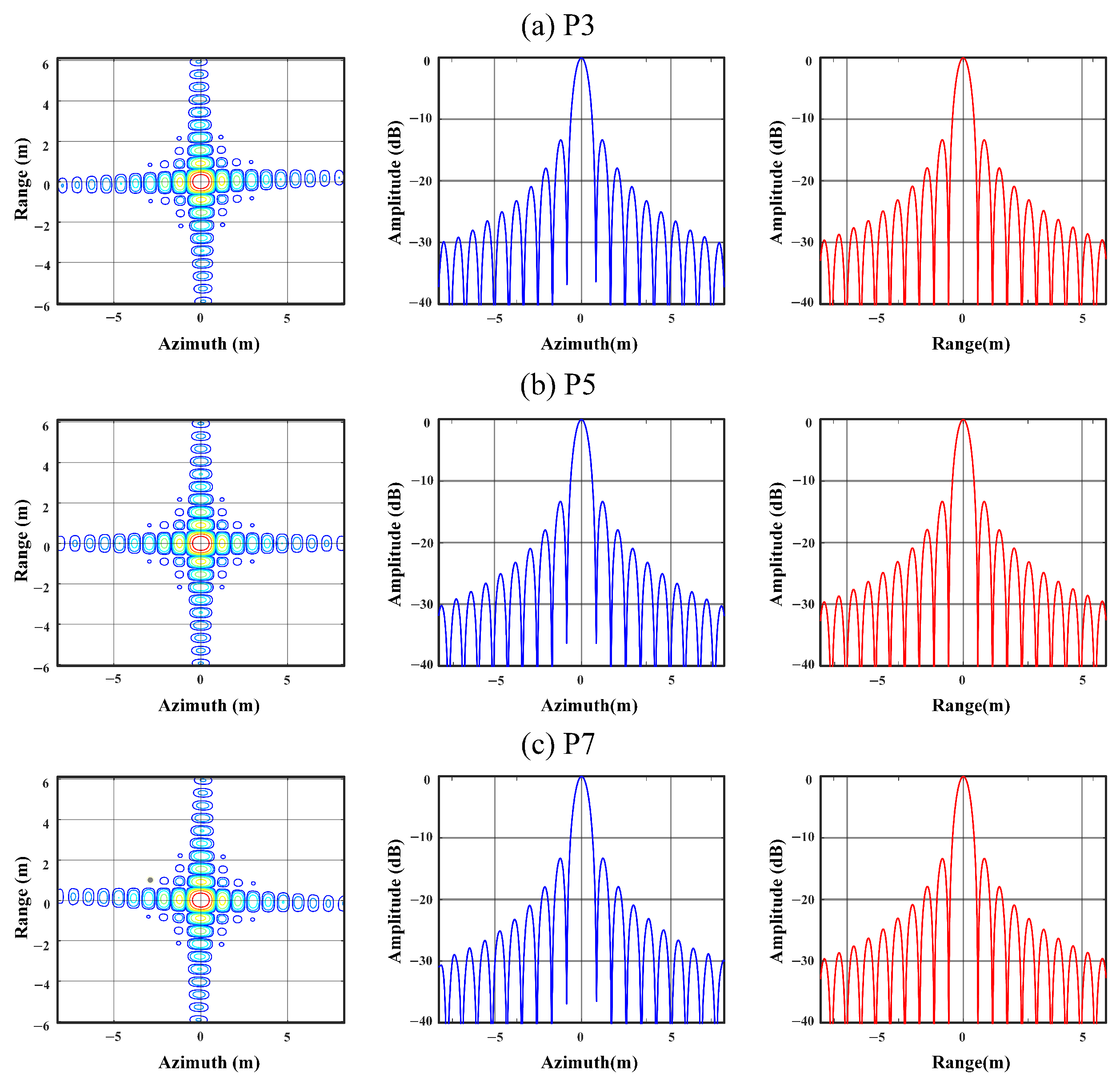
To verify the accuracy and effectiveness of the proposed algorithm, both simulation experiments and real data experiments are conducted in the following sections.

6.1. Simulation

A total of three sets of experiments were designed (marked as simulations 1, 2 below). In simulation 1, both the range and azimuth resolution were 0.1 m, with range and azimuth swaths of 10 km each and an antenna azimuth length of 1m in spotlight mode. The remaining simulation parameters are as shown in Table 1. In simulation 2, both the range resolution and azimuth resolution were 0.2 m, with range and azimuth swaths of 20 km each and an antenna azimuth length of 3.2 m in sliding spotlight mode. The remaining simulation parameters are as shown in Table 1. Figure 30 illustrates the scene and target layout diagrams corresponding to the three sets of simulation experiments.

Based on the analysis in Section 5, the parameters for analyzing the spatial variation obtained from the three sets of simulations are listed in

Table 2. The parameters of the three sets of simulation experiments for spatial variation analysis.

Parameter	Simulation 1	Simulation 2
$B_r$($\mathrm{MHz}$)	1328.08	664.04
$B_a$ ($\mathrm{Hz}$)	62,768.00	31,384.00
$V_s$ ($\mathrm{m}/\mathrm{s}$)	7084.42	7084.42
$R_{\mathrm{ref}}$ ($\mathrm{km}$)	588.76	588.76
$L_{\mathrm{azim},\mathrm{noavRCM}}$ ($\mathrm{km}$)	29.90	241.50
$L_{\mathrm{azim},\mathrm{noavAPM},\mathrm{k}21}$ ($\mathrm{km}$)	1.86	7.49
$L_{\mathrm{azim},\mathrm{noavAPM},\mathrm{k}22}$ ($\mathrm{km}$)	164.27	329.56
$L_{\mathrm{azim},\mathrm{noavAPM},\mathrm{k}31}$ ($\mathrm{km}$)	344.08	2778.22

. According to the last four rows of the table, it can be concluded that all three sets of simulation experiments need to consider the influence of $k_{2,a1}$ on ${\varphi }_0$, while other azimuth spatial variations no longer need to be considered.

The parameters for the three sets of simulation experiments corresponding to the analysis of spatial variation are shown in Table 2.

To more prominently demonstrate the effectiveness of the algorithm proposed in this paper, we adopt the algorithm from [22] as a comparison (referred to as the referenced algorithm below). To be more precise, the referenced algorithm does not correct for azimuth spatial variation, whereas the algorithm proposed in this paper corrects for azimuth spatial variation using ANCS based on the referenced algorithm. Figure 31 and Figure 32 respectively, show the imaging results of the referenced algorithm for simulations 1 and 2. To more clearly observe the differences at various positions in the scene, points $P_3$, $P_5$, and $P_7$ are selected for the presentation of the results of each simulation. In each figure, (a), (b), and (c), respectively, represent the two-dimensional focused images, azimuth profiles, and range profiles of $P_3$, $P_5$, and $P_7$. From the figures, it can be observed that for these three sets of simulations, the impact of azimuth spatial variation is non-negligible, and the imaging quality using the referenced algorithm is not satisfactory.

The imaging results of the proposed algorithm presented in Figure 33 and Figure 34 show the imaging results of simulations 1 and 2, respectively. In each figure, (a), (b), and (c) represent the two-dimensional focused images, azimuth profiles, and range profiles of $P_3$, $P_5$, and $P_7$, respectively. It can be observed from the figures that the effects of azimuth spatial variation are almost completely eliminated after ANCS processing, and excellent imaging results are achieved in all three sets of simulations.

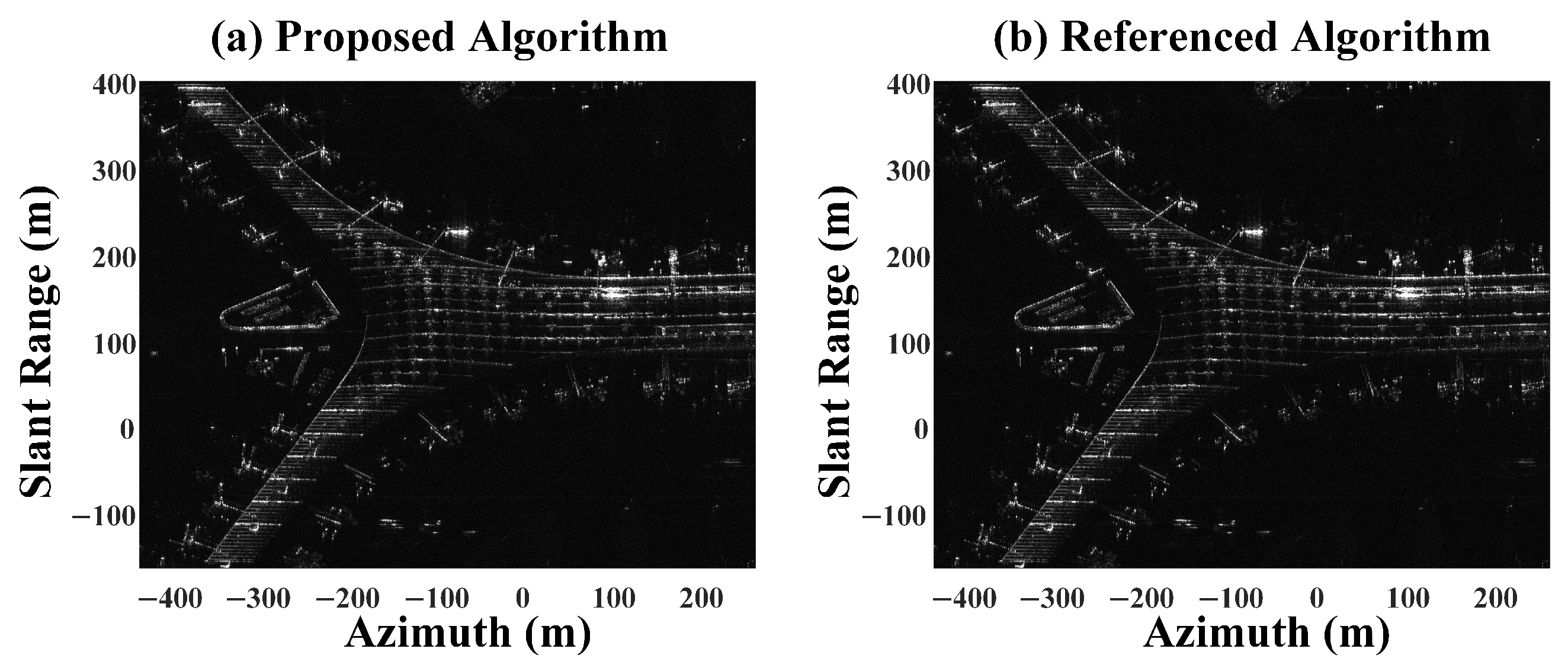
6.2. Processing of Real Data

To further demonstrate the effectiveness of the proposed algorithm, we conducted imaging verification using the same measured data as in [22]. The data were acquired by the GF-3 satellite, with an orbital altitude of approximately 755 km [23]. The transmitted signal is in the C-band, and the radar operates in spotlight mode, achieving a nominal resolution of 1 m in both the azimuth and range (ground range) dimensions, with a nominal swath width of 10 km.

First, we analyze the imaging parameters using the two-dimensional spatial variation analysis method proposed in this paper, with the spatial-variance-related parameters shown in

Table 3. The parameters of real data experiments for spatial variation analysis.

Parameter	Value
$B_r$($\mathrm{MHz}$)	177.08
$B_a$ ($\mathrm{Hz}$)	7984.61
$V_z$ ($\mathrm{m}/\mathrm{s}$)	6756.13
$R_{\mathrm{ref}}$ ($\mathrm{km}$)	8270.36
$L_{\mathrm{azim},\mathrm{noavRCM}}$ ($\mathrm{km}$)	3705.14
$L_{\mathrm{azim},\mathrm{noavAPM},\mathrm{k}21}$ ($\mathrm{km}$)	54.80
$L_{\mathrm{azim},\mathrm{noavAPM},\mathrm{k}22}$ ($\mathrm{km}$)	652.91
$L_{\mathrm{azim},\mathrm{noavAPM},\mathrm{k}31}$ ($\mathrm{km}$)	16,683.69

. From the table, it can be observed that the maximum observable swaths are all greater than the actual observed azimuth swath, thus allowing us to disregard the influence of azimuth spatial variation.

However, to validate the effectiveness of the imaging algorithm presented in this paper, we still conducted imaging experiments using both the reference algorithm and the proposed algorithm. Firstly, we conducted a point target simulation using its satellite parameters and radar parameters, with the scene setup identical to Figure 30a. Figure 35 and Figure 36 show the imaging results of the referenced algorithm and the proposed algorithm, respectively.

Table 4. Point target simulation imaging result metrics using GF-3 real data parameters.

Algorithm	Target	Azimuth			Range
		IRW	PSLR	ISLR	IRW	PSLR	ISLR
Reference Algorithm	$P_3$	0.7446	13.1567	10.056	0.5526	13.2506	9.8105
	$P_5$	0.7540	13.2642	10.1049	0.5526	13.2524	9.8135
	$P_7$	0.7629	13.2586	10.1210	0.5515	13.2773	9.8024
Proposed Algorithm	$P_3$	0.7429	13.2658	10.1177	0.5526	13.2593	9.8146
	$P_5$	0.7540	13.2642	10.1049	0.5526	13.2554	9.8136
	$P_7$	0.7656	13.2416	10.0972	0.5526	13.2770	9.8010

compares the imaging metrics of the two algorithms. The range resolution is the slant-range resolution and has not been converted to ground-range resolution.

From the figures and table, the following conclusions can be drawn: (1) In the comparative algorithm’s imaging results, the worst peak sidelobe ratio of the azimuth profile is 13.15 dB, exceeding the threshold of 13 dB set in [22]. Therefore, under these parameter conditions, the impact of azimuth spatial variation can generally be ignored. (2) However, azimuth spatial variation still reduces the PSLR; thus, after correction with the proposed algorithm, the imaging quality can also be improved.

Finally, we deal with these real data acquired by GF-3. Figure 37 presents the imaging results of the entire scene. For detailed analysis, we selected two representative regions (marked by red boxes in Figure 37): one from the center of the scene and the other from the edge. Enlarged views of these regions are shown in Figure 38 and Figure 39, respectively. Figure 38a and Figure 39a display the imaging results obtained by the proposed algorithm, while Figure 38b and Figure 39b show the imaging results from the reference algorithm.

7. Discussion

To further demonstrate the effectiveness of the proposed algorithm, we analyze the imaging result metrics of the aforementioned two sets of simulation experiments, which are presented in

Table 5. Evaluation metrics of imaging quality in simulation 1.

Algorithm	Target	Azimuth			Range
		IRW	PSLR	ISLR	IRW	PSLR	ISLR
Reference Algorithm	$P_3$	0.1021	12.7699	9.1658	0.1000	13.2288	10.0081
	$P_5$	0.0997	13.3532	10.6065	0.1000	13.2621	9.9797
	$P_7$	0.0977	12.5516	9.2375	0.1000	13.2482	9.8236
Proposed Algorithm	$P_3$	0.0992	13.3422	10.5922	0.1000	13.2705	9.9382
	$P_5$	0.0997	13.2634	10.4491	0.1000	13.2790	9.9282
	$P_7$	0.1000	13.2904	10.6456	0.1000	13.2727	9.9384

and

Table 6. Evaluation metrics of imaging quality in simulation 2.

Algorithm	Target	Azimuth			Range
		IRW	PSLR	ISLR	IRW	PSLR	ISLR
Reference Algorithm	$P_3$	0.1844	12.8206	9.7908	0.1996	13.2570	9.7928
	$P_5$	0.1998	13.2848	10.3101	0.1996	13.2536	9.7913
	$P_7$	0.2108	13.2212	10.3475	0.2000	13.2479	9.7831
Proposed Algorithm	$P_3$	0.1840	13.2188	10.2805	0.1996	13.2545	9.7910
	$P_5$	0.1998	13.2853	10.3105	0.1996	13.2544	9.7916
	$P_7$	0.2099	13.2951	10.2949	0.2000	13.2554	9.7868

, respectively. From these metrics, in addition to confirming that the proposed algorithm adequately corrects the azimuth spatial variation and achieves better imaging results, we can also obtain more information: (1) From the metrics of range dimension in the two sets of experiments, it can be observed that the referenced algorithm is so effective in correcting spatial range variation that, regardless of whether the azimuth spatial variation is removed, it can achieve good imaging quality in the range dimension. (2) By comparing the metrics of $P_3$ and $P_7$ in Table 6, it can be found that the impact of azimuth spatial variation on $P_3$ is greater than that on $P_7$, which also confirms that, under the same parameters, the azimuth spatial variation increases with ${\theta }_{\mathrm{off}}$(or $R_0$), as shown in Figure 11.

Furthermore, we evaluated the imaging quality of the two algorithms on the real data. From a visual comparison standpoint, the results of these two algorithms are very similar and difficult to distinguish. To provide a clearer comparison of imaging quality, we selected commonly used metrics for evaluating SAR images: contrast and entropy. Higher contrast and lower entropy indicate better imaging quality. Using these two metrics, we assessed the images in Figure 38 and Figure 39, with the results presented in

Table 7. Imaging quality of real data.

Region	Algorithm	Contrast	Entropy
Region 1	Reference Algorithm	7.1272	1.6524
	Proposed Algorithm	7.1274	1.6518
Region 2	Reference Algorithm	7.3634	1.6062
	Proposed Algorithm	7.4450	1.5920

. Based on the results in the table, we can observe that after azimuth spatial variation correction, the algorithm proposed in this paper achieves better imaging quality.

8. Conclusions

Benefiting from the slant range model based on the zero-Doppler moment established at the beginning of this paper, the two-dimensional spatial variation of HRWS spaceborne SAR will only originate from the satellite–ground geometry and will be independent of beam rotation. This significantly reduces its azimuth spatial variation component and makes it applicable to various high-resolution imaging modes.

Given the realistic scenario where the satellite trajectory in the ECEF frame is a non-coplanar curve, this paper establishes a new spaceborne SAR geometric model: CUSM. Based on this model, by developing quantitative descriptions of the satellite trajectory and the slant range history, we are able to quantitatively analyze and model the two-dimensional spatial variation characteristics of HRWS spaceborne SAR.

It is precisely for this reason that we can precisely analyze the specific impact and extent of two-dimensional spatial variation. By establishing thresholds for different types of azimuth spatial variation, we can derive theoretical guidance on when and which type of azimuth spatial variation needs to be considered.

Subsequently, we propose a two-dimensional spatial variation correction method that combines range blocking and azimuth NCS processing. This method does not require iteration and interpolation, offering high computational efficiency. Finally, we also demonstrate the effectiveness and broad applicability of this algorithm through multiple sets of simulation experiments and real data experiments.

References

1. Wu, C.; Liu, K.Y.; Jin, M. Modeling and a Correlation Algorithm for Spaceborne SAR Signals. IEEE Trans. Aerosp. Electron. Syst. 1982, AES-18, 563–575. [Google Scholar] [CrossRef]
2. Eldhuset, K. A New Fourth-Order Processing Algorithm for Spaceborne SAR. IEEE Trans. Aerosp. Electron. Syst. 1998, 34, 824–835. [Google Scholar]
3. Eldhuset, K. Ultra High Resolution Spaceborne SAR Processing. IEEE Trans. Aerosp. Electron. Syst. 2004, 40, 370–378. [Google Scholar]
4. Kim, J.-H.; Younis, M.; Prats-Iraola, P.; Gabele, M.; Krieger, G. First Spaceborne Demonstration of Digital Beamforming for Azimuth Ambiguity Suppression. IEEE Trans. Geosci. Remote Sens. 2012, 51, 579–590. [Google Scholar] [CrossRef]
5. Prats-Iraola, P.; Scheiber, R.; Rodriguez-Cassola, M.; Mittermayer, J.; Wollstadt, S.; De Zan, F.; Bräutigam, B.; Schwerdt, M.; Reigber, A.; Moreira, A. On the Processing of Very High Resolution Spaceborne SAR Data. IEEE Trans. Geosci. Remote Sens. 2014, 52, 6003–6016. [Google Scholar]
6. Xiang, T.; Zhu, D.; Xu, F. Processing of Ultra-High Resolution Spaceborne Spotlight SAR Data Based on One-Step Motion Compensation. In Proceedings of the IGARSS 2018–2018 IEEE International Geoscience and Remote Sensing Symposium, Valencia, Spain, 22–27 July 2018; pp. 8933–8936. [Google Scholar]
7. Liang, D.; Zhang, H.; Fang, T.; Deng, Y.; Yu, W.; Zhang, L.; Fan, H. Processing of Very High Resolution GF-3 SAR Spotlight Data with Non-Start–Stop Model and Correction of Curved Orbit. IEEE J. Sel. Top. Appl. Earth Obs. Remote Sens. 2020, 13, 2112–2122. [Google Scholar]
8. Sun, G.-C.; Liu, Y.; Xiang, J.; Liu, W.; Xing, M.; Chen, J. Spaceborne Synthetic Aperture Radar Imaging Algorithms: An Overview. IEEE Geosci. Remote Sens. Mag. 2021, 10, 161–184. [Google Scholar]
9. Meng, D.; Huang, L.; Qiu, X.; Li, G.; Hu, Y.; Han, B.; Hu, D. A Novel Approach to Processing Very-High-Resolution Spaceborne SAR Data With Severe Spatial Dependence. IEEE J. Sel. Top. Appl. Earth Obs. Remote Sens. 2022, 15, 7472–7482. [Google Scholar]
10. Mao, X. Spherical Geometry Algorithm for Space-Borne Synthetic Aperture Radar Imaging. IEEE Trans. Geosci. Remote Sens. 2024, 62, 1–15. [Google Scholar]
11. Hernández-Burgos, S.; Gibert, F.; Broquetas, A.; Kleinherenbrink, M.; De la Cruz, A.F.; Gómez-Olivé, A.; García-Mondéjar, A.; i Aparici, M.R. A Fully Focused SAR Omega-K Closed-Form Algorithm for the Sentinel-6 Radar Altimeter: Methodology and Applications. IEEE Trans. Geosci. Remote Sens. 2024, 62, 1–16. [Google Scholar]
12. Shibata, M.; Kuriyama, T.; Hoshino, T.; Nakamura, S.; Kankaku, Y.; Motohka, T.; Suzuki, S. SAR Techniques and SAR Processing Algorithm for ALOS-4. In Proceedings of the IGARSS 2022–2022 IEEE International Geoscience and Remote Sensing Symposium, Kuala Lumpur, Malaysia, 17–22 July 2022; pp. 7449–7451. [Google Scholar]
13. Farquharson, G.; Castelletti, D.; De, S.; Stringham, C.; Yague, N.; Bes, V.C.; Ryu, J.; Goncharenko, Y. The New Capella Space Satellite Generation: Acadia. In Proceedings of the IGARSS 2023–2023 IEEE International Geoscience and Remote Sensing Symposium, Pasadena, CA, USA, 16–21 July 2023; pp. 1513–1516. [Google Scholar]
14. He, F.; Chen, Q.; Dong, Z.; Sun, Z. Processing of Ultrahigh-Resolution Spaceborne Sliding Spotlight SAR Data on Curved Orbit. IEEE Trans. Aerosp. Electron. Syst. 2013, 49, 819–839. [Google Scholar] [CrossRef]
15. Wang, P.; Liu, W.; Chen, J.; Niu, M.; Yang, W. A High-Order Imaging Algorithm for High-Resolution Spaceborne SAR Based on a Modified Equivalent Squint Range Model. IEEE Trans. Geosci. Remote Sens. 2014, 53, 1225–1235. [Google Scholar] [CrossRef]
16. Wu, Y.; Sun, G.-C.; Yang, C.; Yang, J.; Xing, M.; Bao, Z. Processing of Very High Resolution Spaceborne Sliding Spotlight SAR Data Using Velocity Scaling. IEEE Trans. Geosci. Remote Sens. 2015, 54, 1505–1518. [Google Scholar] [CrossRef]
17. Tang, S.; Lin, C.; Zhou, Y.; So, H.C.; Zhang, L.; Liu, Z. Processing of Long Integration Time Spaceborne SAR Data with Curved Orbit. IEEE Trans. Geosci. Remote Sens. 2017, 56, 888–904. [Google Scholar]
18. Liu, W.; Sun, G.-C.; Xia, X.-G.; Chen, J.; Guo, L.; Xing, M. A Modified CSA Based on Joint Time-Doppler Resampling for MEO SAR Stripmap Mode. IEEE Trans. Geosci. Remote Sens. 2018, 56, 3573–3586. [Google Scholar]
19. Guo, Y.; Wang, P.; Chen, J.; Men, Z.; Cui, L.; Zhuang, L. A Novel Imaging Algorithm for High-Resolution Wide-Swath Space-Borne SAR Based on a Spatial-Variant Equivalent Squint Range Model. Remote Sens. 2022, 14, 368. [Google Scholar] [CrossRef]
20. Ding, Z.; Zheng, P.; Li, H.; Zhang, T.; Li, Z. Spaceborne High-Squint High-Resolution SAR Imaging Based on Two-Dimensional Spatial-Variant Range Cell Migration Correction. IEEE Trans. Geosci. Remote Sens. 2022, 60, 1–14. [Google Scholar] [CrossRef]
21. Chen, X.; Hou, Z.; Dong, Z.; He, Z. Performance Analysis of Wavenumber Domain Algorithms for Highly Squinted SAR. IEEE J. Sel. Top. Appl. Earth Obs. Remote Sens. 2023, 16, 1563–1575. [Google Scholar]
22. Hou, Z.; Zhang, Z.; Li, P.; Yun, Z.; He, F.; Dong, Z. Range-Dependent Variance Correction Method for High-Resolution and Wide-Swath Spaceborne Synthetic Aperture Radar Imaging Based on Block Processing in Range Dimension. Remote Sens. 2024, 17, 50. [Google Scholar] [CrossRef]
23. Zhang, Q. System Design and Key Technologies of the GF-3 Satellite. Acta Geod. Cartogr. Sin. 2017, 46, 269–277. [Google Scholar]
Figure 1. Schematic diagram of spaceborne SAR imaging geometry. (In the figure, the red solid line represents the satellite trajectory, the green solid line represents the Earth’s surface, the green dashed line indicates the observation swath, the black solid line denotes the instantaneous beam illumination area, the yellow triangle marks the beam azimuth center plane, the black dash-dotted line shows the connection between satellite and target within the beam azimuth center plane, and the black dashed line represents the zero-Doppler connection between satellite and target).
Remotesensing 17 01262 g001
Figure 2. Schematic diagram of target deployment. (The black rectangle in the figure represents the observation scene coverage, the blue solid lines in (a,b) denote the intersection lines between the beam azimuth center plane and Earth’s surface at different azimuth times, and the red solid line in (c) indicates the intersection line between the zero-Doppler plane and Earth’s surface at different azimuth times.)
Remotesensing 17 01262 g002
Figure 3. Simulation of the target layout in different methods. (a) Target layout results based on the sliding-spotlight mode at the moment of beam center. (b) Target layout results based on the spotlight mode at the moment of beam center. (c) Target layout results for both sliding-spotlight mode and spotlight mode at zero-Doppler moments.
Remotesensing 17 01262 g003
Figure 4. Phase error between the range model and the actual slant range. (a) Simulation results for an azimuth resolution of 0.2 m and an azimuth swath of 20 km. (b) Simulation results for a resolution of 0.1 m and an azimuth swath of 10 km.
Remotesensing 17 01262 g004
Figure 5. Schematic diagram of CUSM. The green solid line represents the Earth’s surface, and the red solid line depicts the satellite’s orbital path. (a) Geometric relationship between the satellite and Earth in the ECI frame. (b) Geometric relationship between the satellite and Earth in the ECEF frame.
Remotesensing 17 01262 g005
Figure 6. Geometric diagram of a satellite’s elliptical orbit. (The red ellipse represents the satellite’s orbit in the orbital coordinate system, the green circle is the circumcircle of the ellipse, the blue point indicates the focus of the ellipse, a is the semi-major axis, f is the true anomaly, E is the eccentric anomaly, and M is the mean anomaly).
Remotesensing 17 01262 g006
Figure 7. The (a) Error between E obtained by the series inversion method and the true value. (b) Error between Equation (10) obtained by the series inversion method and the true value. (c) Error between Equation (11) obtained by the series inversion method and the true value.
Remotesensing 17 01262 g007
Figure 8. Variation of k 2 , a 1 , k 2 , a 2 , and k 3 , a 1 with i. (a) k 2 , a 1 . (b) k 2 , a 2 . (c) k 3 , a 1 .
Remotesensing 17 01262 g008
Figure 9. Variation of k 2 , a 1 , k 2 , a 2 , and k 3 , a 1 with ω . (a) k 2 , a 1 . (b) k 2 , a 2 . (c) k 3 , a 1 .
Remotesensing 17 01262 g009
Figure 10. Variation of k 2 , a 1 , k 2 , a 2 , and k 3 , a 1 with e. (a) k 2 , a 1 . (b) k 2 , a 2 . (c) k 3 , a 1 .
Remotesensing 17 01262 g010
Figure 11. Variation of k 2 , a 1 , k 2 , a 2 , and k 3 , a 1 with θ off . (a) k 2 , a 1 . (b) k 2 , a 2 . (c) k 3 , a 1 .
Remotesensing 17 01262 g011
Figure 12. Variation of k 2 , a 1 , k 2 , a 2 , and k 3 , a 1 with a. (a) k 2 , a 1 . (b) k 2 , a 2 . (c) k 3 , a 1 .
Remotesensing 17 01262 g012
Figure 13. Impact of two-dimensional spatial variation on RCM. (a) Only existing k 2 , a 1 . (b) Only existing k 2 , a 2 . (c) Only existing k 3 , a 1 .
Remotesensing 17 01262 g013
Figure 14. Impact of azimuth spatial variation on RCM. (a) Only existing k 2 , a 1 . (b) Only existing k 2 , a 2 . (c) Only existing k 3 , a 1 .
Remotesensing 17 01262 g014
Figure 15. Variation of maximum swath with resolution when ignoring the azimuth spatial variation of RCM. (a) Numerical plot. (b) Contour plot. (c) Logarithmic plot.
Remotesensing 17 01262 g015
Figure 16. Variation of maximum swath with resolution when ignoring the azimuth spatial variation of RCM (while maintaining equivalent range and azimuth resolutions). (a) Large view. (b) Zoomed-in view.
Remotesensing 17 01262 g016
Figure 17. Impact of two-dimensional spatial variation on AMP. (a) Only existing k 2 , a 1 . (b) Only existing k 2 , a 2 . (c) Only existing k 3 , a 1 .
Remotesensing 17 01262 g017
Figure 18. Impact of azimuth spatial variation on AMP. (a) Only existing k 2 , a 1 . (b) Only existing k 2 , a 2 . (c) Only existing k 3 , a 1 .
Remotesensing 17 01262 g018
Figure 19. Variation of maximum swath with resolution when ignoring the azimuth spatial variation of APM (in the case where only k 2 , a 1 exists). (a) Large view. (b) Zoomed-in view.
Remotesensing 17 01262 g019
Figure 20. Variation of maximum swath with resolution when ignoring the azimuth spatial variation of APM (in the case where only k 2 , a 2 exists). (a) Large view. (b) Zoomed-in view.
Remotesensing 17 01262 g020
Figure 21. Variation of maximum swath with resolution when ignoring the azimuth spatial variation of APM (in the case where only k 3 , a 1 exists). (a) Large view. (b) Zoomed-in view.
Remotesensing 17 01262 g021
Figure 22. Variation of the four maximum azimuth swaths with azimuth resolution and the semi-major axis. (a) L azim , noavRCM . (b) L azim , noavAPM , k 21 . (c) L azim , noavAPM , k 22 (d) L azim , noavAPM , k 31 .
Remotesensing 17 01262 g022
Figure 23. Variations of the four maximum azimuth swaths with azimuth resolution and eccentricity. (a) L azim , noavRCM . (b) L azim , noavAPM , k 21 . (c) L azim , noavAPM , k 22 . (d) L azim , noavAPM , k 31 .
Remotesensing 17 01262 g023
Figure 24. Variation of the four maximum azimuth swaths with azimuth resolution and inclination. (a) L azim , noavRCM . (b) L azim , noavAPM , k 21 . (c) L azim , noavAPM , k 22 . (d) L azim , noavAPM , k 31 .
Remotesensing 17 01262 g024
Figure 25. Variation of the four maximum azimuth swaths with azimuth resolution and the argument of periapsis. (a) L azim , noavRCM . (b) L azim , noavAPM , k 21 . (c) L azim , noavAPM , k 22 . (d) L azim , noavAPM , k 31 .
Remotesensing 17 01262 g025
Figure 26. Variation of the four maximum azimuth swaths with azimuth resolution and look angle. (a) L azim , noavRCM . (b) L azim , noavAPM , k 21 . (c) L azim , noavAPM , k 22 . (d) L azim , noavAPM , k 31 .
Remotesensing 17 01262 g026
Figure 27. Variation of the four maximum azimuth swaths with azimuth resolution and wavelength. (a) L azim , noavRCM . (b) L azim , noavAPM , k 21 . (c) L azim , noavAPM , k 22 . (d) L azim , noavAPM , k 31 .
Remotesensing 17 01262 g027
Figure 28. Flowchart of the proposed algorithm. Yellow, purple and blue dashed boxes represent spatial range variation correction, azimuth NCS processing, and azimuth compression, respectively.
Remotesensing 17 01262 g028
Figure 29. Imaging metrics for different length of azimuth blocks. (a) PSLR (b) ISLR (c) Azimuth Resolution.
Remotesensing 17 01262 g029
Figure 30. Schematic diagram of the scenarios and target deployment corresponding to the three sets of simulation experiments. (a) Simulation 1. (b) Simulation 2.
Remotesensing 17 01262 g030
Figure 31. The imaging results of the referenced algorithm in simulation 1. (a) P3. (b) P5. (c) P7.
Remotesensing 17 01262 g031
Figure 32. The imaging results of the referenced algorithm in simulation 2. (a) P3. (b) P5. (c) P7.
Remotesensing 17 01262 g032
Figure 33. The imaging results of the proposed algorithm in simulation 1. (a) P3. (b) P5. (c) P7.
Remotesensing 17 01262 g033
Figure 34. The imaging results of the proposed algorithm in simulation 2. (a) P3. (b) P5. (c) P7.
Remotesensing 17 01262 g034
Figure 35. Point target simulation imaging results using GF-3 real data parameters (reference algorithm). (a) P3. (b) P5. (c) P7.
Remotesensing 17 01262 g035
Figure 36. Point target simulation imaging results using GF-3 real data parameters (proposed algorithm). (a) P3. (b) P5. (c) P7.
Remotesensing 17 01262 g036
Figure 37. Imaging results of GF-3 (whole scene). In the figure, the red box marked with the number “1” represents the selected region at the center of the scene, while the red box marked with the number “2” represents the selected region at the edge of the scene.
Remotesensing 17 01262 g037
Figure 38. Imaging results of GF-3 (region 1). (a) Reference algorithm. (b) Proposed algorithm.
Remotesensing 17 01262 g038
Figure 39. Imaging results of GF-3 (region 2). (a) Reference algorithm. (b) Proposed algorithm.
Remotesensing 17 01262 g039